An Algorithm to Extract the Boundary and Center of EUV Solar Image Based on Sobel Operator and FLICM

China Academy of Space Technology (Xi’an), Xi’an 710100, China
*
Author to whom correspondence should be addressed.
Photonics 2022, 9(12), 889; https://doi.org/10.3390/photonics9120889
Submission received: 18 October 2022
/
Revised: 16 November 2022
/
Accepted: 21 November 2022
/
Published: 22 November 2022
(This article belongs to the Special Issue Advanced Polarimetry and Polarimetric Imaging)
Abstract
:An algorithm to extract the disk boundary and center of EUV solar image using the Sobel operator, Fuzzy Local Information C-Means Clustering algorithm (FLICM), and the least square circle fitting method is proposed in this paper. The Sobel operator can determine the solar disk boundary preliminarily, and then the image is processed further using the FLICM algorithm. After the background is removed based on the clustered image and the boundary points can be highlighted, these points are fitted using the least square circle fitting method as the final boundary circle. The solar data used in this paper was from the observation of the Solar Dynamics Observatory Atmospheric Imaging Assembly (SDO/AIA) instrument. The 2523 19.3 nm solar images covering solar minimum, moderate solar activity, and more active suns were calculated using the proposed algorithm to analyze the accuracy statistically. The statistical comparison results demonstrate that the method is accurate and effective. This method can support the processing of solar EUV images and serve the operational system of a space weather forecast.
1. Introduction
Imaging the sun in extreme ultraviolet (EUV) band from space is an important approach to monitoring a hot coronal plasma in active solar phenomena. It can improve the forecast of space weather and early warnings of possible impacts on the Earth’s environment. Space-borne optical remote instruments for the Sun have been developed for more than 40 years, and many EUV imaging instruments have been launched to study solar atmospheric dynamics. The Extreme-ultraviolet Imaging Telescope (EIT) onboard the Solar and Heliospheric Observatory (SOHO) was launched in 1995 to observe the corona and transition region on the solar disk in 17.1 nm (Fe IX), 19.5 nm (Fe XII), 28.4 nm (Fe XV) and 30.4 nm (He II) [1,2,3]. In 1998, the Transition Region and Coronal Explorer (TRACE) mission with three EUV imaging channels was launched to image the solar corona at 17.1 nm, 19.5 nm, and 28.4 nm for diagnosis of coronal plasmas between 105 K and 106 K [4,5]. As the successor to TRACE, the National Aeronautics and Space Administration (NASA) launched the Solar Dynamics Observatory (SDO) mission in 2010, and the Atmospheric Imaging Assembly (AIA) onboard SDO has provided near-continuous monitoring of the Sun in 7 narrowband EUV channels [6,7]. The Extreme Ultraviolet Imager (EUI), equipped in the Solar Orbiter mission, was launched last year, which aims to provide full-disk EUV and high-resolution EUV and Lyman-α imaging of the solar atmosphere by imaging the three spectral lines of 17.4 nm, 30.4 nm and 121.6 nm [8,9]. In 2021, the solar X-ray and EUV telescope, on board the Fengyun-3E satellite, was launched in China, which imaged the sun at 19.5 nm [10]. These instruments accumulated a large number of solar EUV images for solar study.
Before the solar image is released, it needs to go through a lot of processes and corrections. Among them, image positioning is an extremely important step [11,12,13]. Finding the accurate center and radii is not a trivial problem for solar EUV images since the corona is complex. For solar images in visible and infrared bands, the boundary can be calculated using solar limb darkening [14,15,16]. However, this method is not suitable for EUV images. Also, finding accurate limb positions for EUV images was challenging for the AIA team. After some experimentation, they found techniques that work on all AIA channels except 30.4 nm (which has a particularly noisy limb). The EUV images were processed with Sobel transform after a 3-pixel Gaussian smooth. To isolate a limb signal better, they calculated a radial direction for the first derivative between ±5° around the rough boundary. The next step is to use these points to get an estimate of the limb and use it to eliminate bad points from the set. Finally, a least squares fit finds the optimal circle that intersects a maximum number of the remaining points [17,18].
This paper described a method to extract the center and boundary of solar EUV images based on the Sobel operator, FLICM algorithm, and the least square circle fitting. The EUV images are preprocessed with the Sobel operator to find the rough boundaries. Then, the FLICM algorithm is used to cluster images and remove the discrete background. After the two steps, the extreme points of the boundary will be fitted using the least square circle fitting method. The outline of this paper is as follows. The data sets used in this paper will be introduced in Section 2. The Sobel operator and FLICM algorithm will be described in detail in Section 3 and Section 4, respectively. The fitting results will be displayed in Section 5, and the statistical analysis of extraction results will be discussed in Section 6. Finally, a conclusion will be given in Section 7.
2. Data Sets
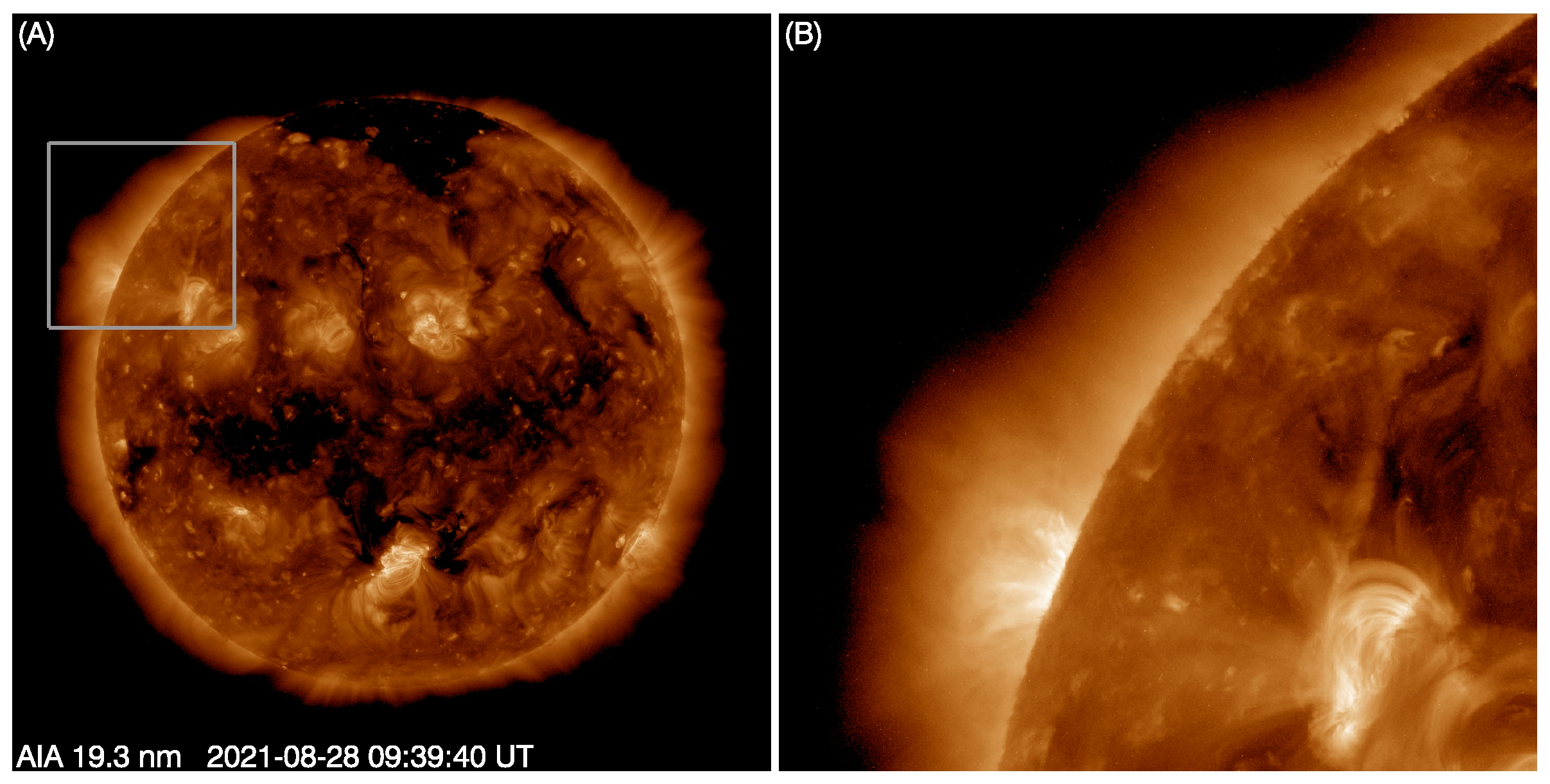
The solar EUV images used in this study were obtained by the Solar Dynamics Observatory Atmospheric Imaging Assembly (SDO/AIA) instrument [6,7]. SDO/AIA is the follow-on to the extremely successful Transition Region and Coronal Explorer (TRACE) mission, which consists of 4 individual telescopes. Each telescope consists of a mirror system coated in halves, each of which responds to a different portion of the solar spectrum, resulting in a virtual system of 8 distinct telescopes. The field of view of the AIA telescopes is 41 arcmins, large enough to encompass the full sun. The AIA is to provide narrow-band imaging of seven extreme ultraviolet (EUV) band passes centered on specific lines: Fe XVIII (9.4 nm), Fe VIII, XXI (13.1 nm), Fe IX (17.1 nm), Fe XII, XXIV (19.3 nm), Fe XIV (21.1 nm), He II (30.4 nm), and Fe XVI (33.5 nm), at a resolution consistent with 0.6 arcsec detector pixels, once every 10 s. One telescope observes C IV (near 160 nm) and the nearby continuum (170 nm) and has a filter that observes in visible to enable alignment with images from other telescopes. The AIA was launched with an SDO mission on 11 February 2010. Operating in geosynchronous orbit, the AIA has observed and accumulated a large amount of solar data so far. The data used in this paper is the Lev 1 product of SDO/AIA from https://sdac.virtualsolar.org/cgi/search (21 November 2022). There are 1076 solar 19.3 nm images from 1 August 2021 to 31 October 2021, 718 images with a time interval of 12 h in all of 2014, and 729 images with a time interval of 12 h in all of 2019 were calculated in this paper. Figure 1A shows the 19.3 nm solar image observed by AIA at 09:39:40 UTC on 28 August 2021. Figure 1B is the local enlarged image in the rectangular box in Figure 1A, which is used to display the boundary information of the EUV image.
3. Sobel Operator
To extract the disk boundary of the EUV solar image, the first step is to recalculate the image using the Sobel operator. The Sobel operator is an edge detection with the first derivative [19,20]. In the process of the algorithm, a 3 × 3 template is used as the kernel to perform convolution and operation with each pixel in the image. Then a suitable threshold is selected to extract the edge. Technically, it is a discrete differentiation operator, computing an approximation of the gradient of the image intensity function. At each point in the image, the result of the Sobel operator is either the corresponding gradient vector or the norm of this vector. Sobel operator is the partial derivative of Fx,y as the central computing 3 × 3 neighborhood at x, y direction. To suppress the noise, a certain weight is correspondingly increased on the center point, and its digital gradient approximation equations may describe as follows:
The size of its gradient is
The convolution template operator is as follows:
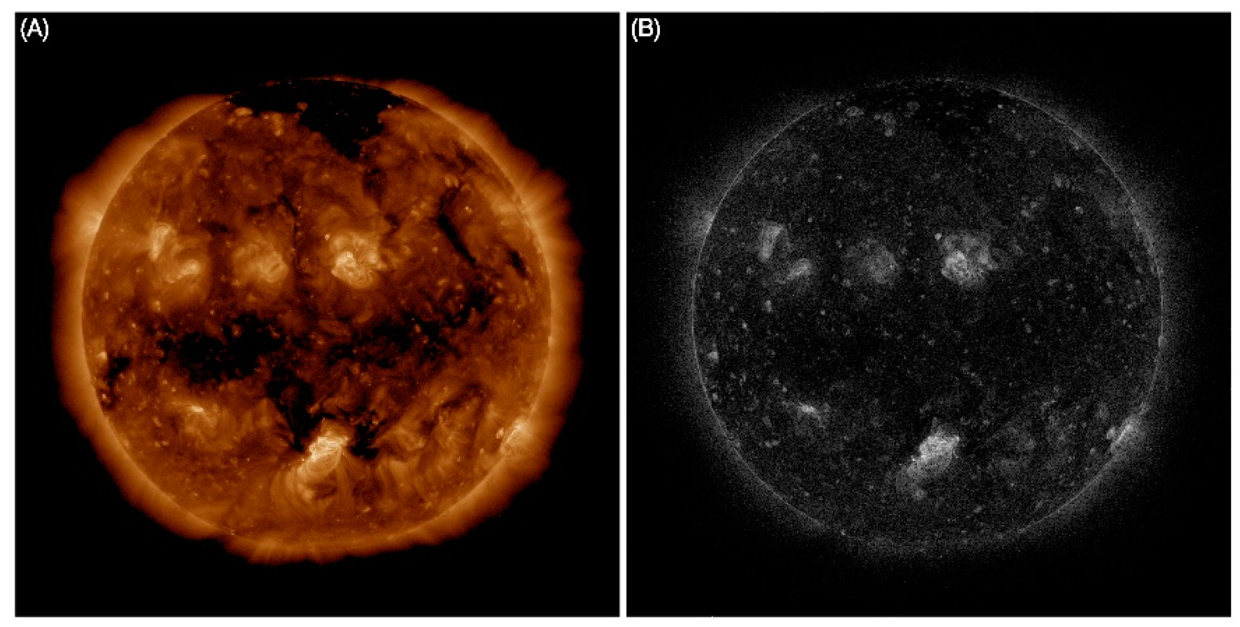
When calculating the edge of the image, the horizontal template Tx and the vertical template Ty are used to convolute with the image. Then, two gradient matrices of the same size as the original image can be obtained. Finally, the total gradient value can be calculated by adding the two matrices, and the edge can be obtained by the threshold method. The result is shown in Figure 2, while Figure 2A is the original EUV image, and Figure 2B is the edge distribution detected by the Sobel operator. As shown in Figure 2, the location of the solar disk boundary is further enhanced.
4. FLICM Algorithm
In this section, a robust Fuzzy Local Information C-Means Clustering algorithm (FLICM) is used to further extract the basic positional information of solar disk boundary [21,22]. This algorithm incorporates local spatial and gray-level information in a fuzzy way to preserve robustness and noise insensitiveness by adding a novel fuzzy factor
to the squared error objective function
where N is the total number of pixels, c is the number of clusters with 2 ≤ c < N, xi is the gray level of the ith pixel, which is the center of the local window (e.g., 3 × 3 pixels), vk is the prototype of the center of cluster k, uki is the degree of the membership of xi in the kth cluster, m is a weighting exponent on each fuzzy membership that determines the amount of fuzziness of the resulting classification and is usually set to be 2, Ni stands for the set of neighbors falling into a local window around pixel xi, and dij is the spatial Euclidean distance between pixels i and j. The necessary conditions for Jm to be at its minimal local extreme, with respect to uki and vk are obtained in the following formulas:
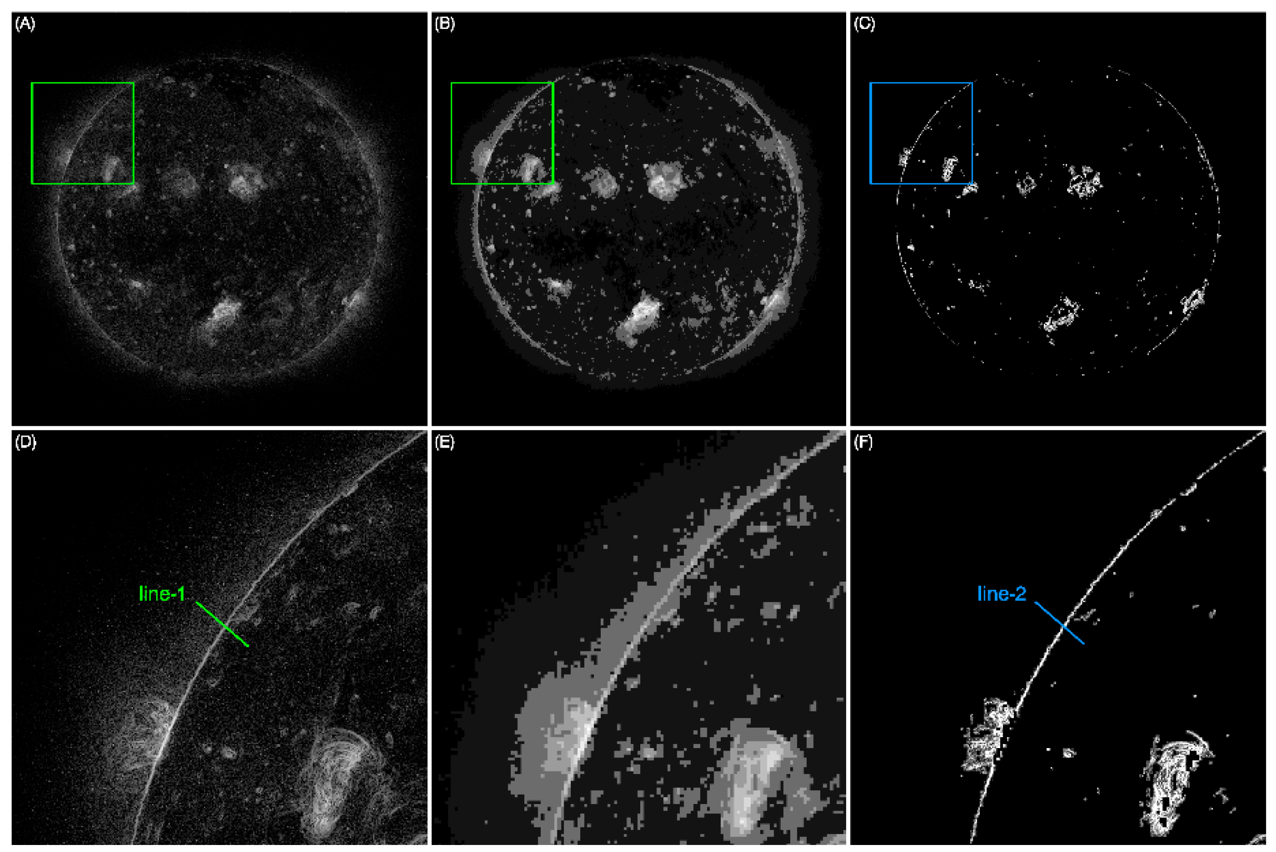
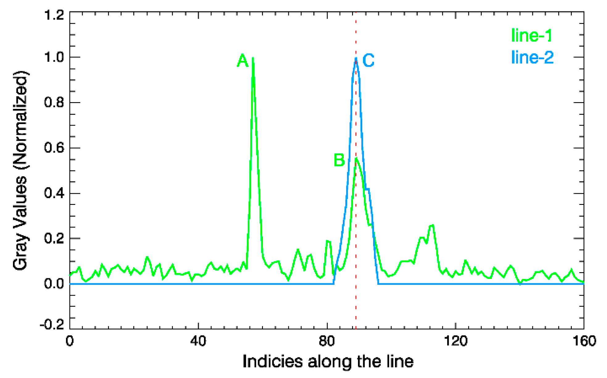
In this paper, the solar image after the Sobel operator calculation will be clustered into 10 categories using the FLICM algorithm (c was set to 10), and the pixels lower than the median gray value will be zeroed. As shown in Figure 3, Figure 3B is the result after the FLICM algorithm operation, and after background removal, the image in Figure 3C. Figure 3D–F is a partially enlarged view of the rectangular boxes in Figure 3A–C. The green line-1 and blue line-2 are selected to verify that the algorithm can effectively remove interference points near the boundary. The normalized gray values vs. pixels along the lines are given in Figure 4, and the red dotted line marks the location of the solar disk boundary along the line. Mass calculations have proved that this method can efficiently remove the interference points nearby the boundary, and Figure 3C will be further used to find the disk boundary.
5. Least Square Circle Fitting
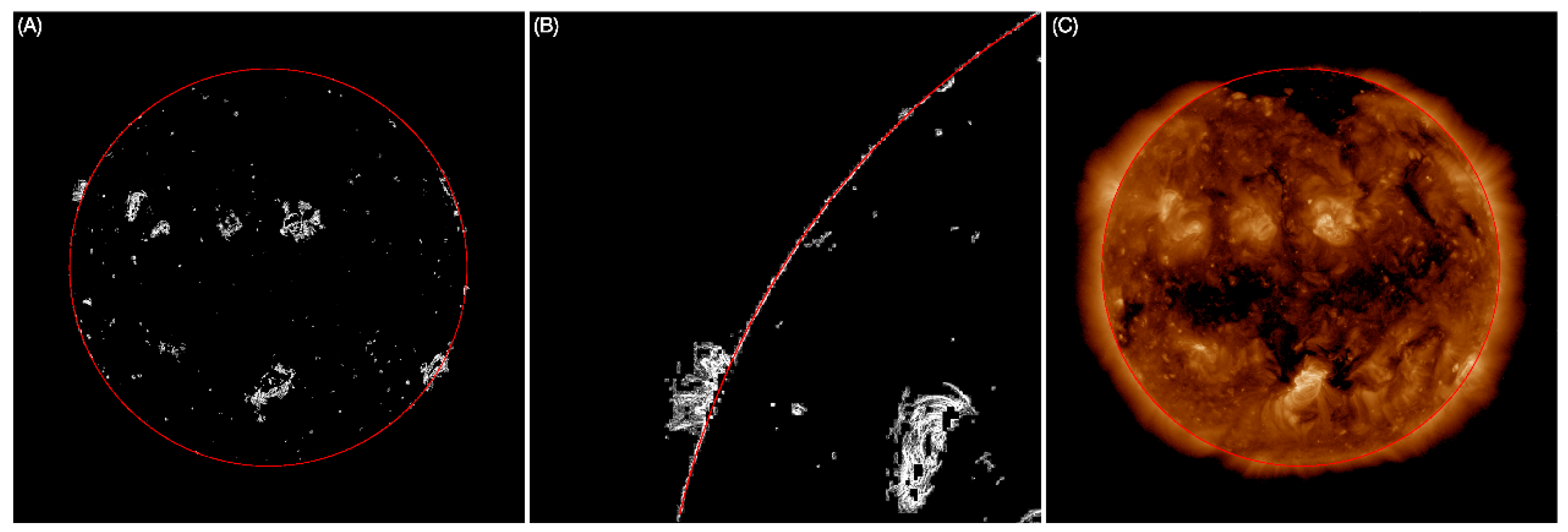
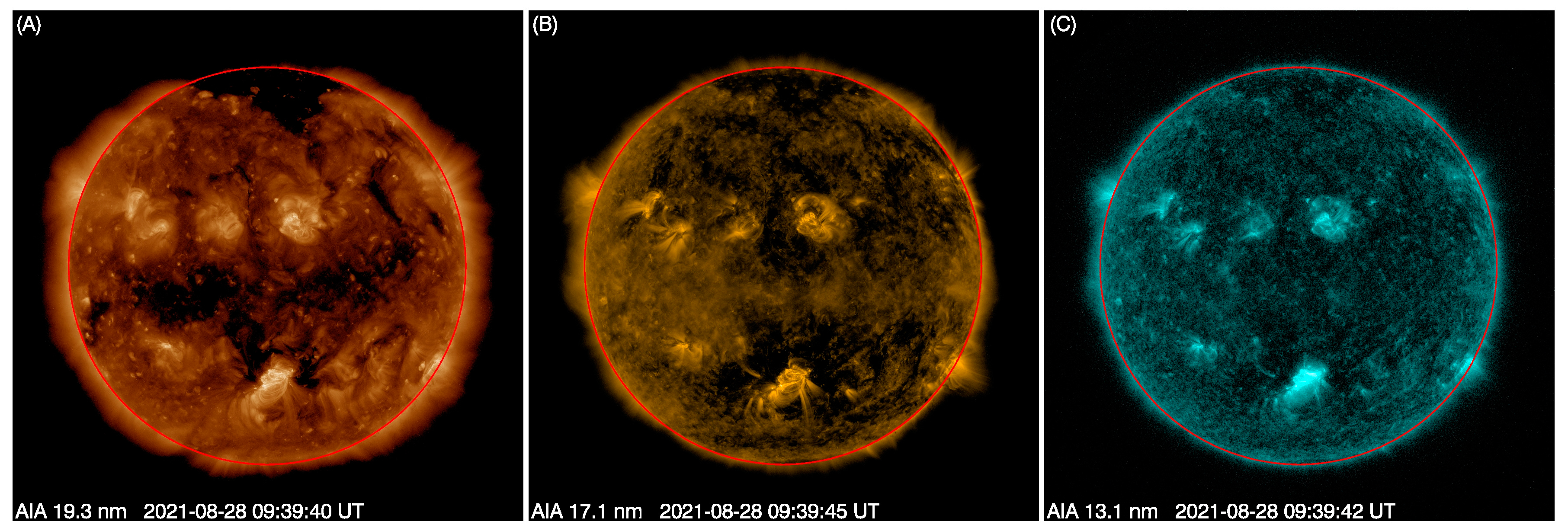
Drawing lines from the image center from 0° to 360°, and the step size is set to 0.5°. Since the CCD size of AIA is 4096 × 4096, the image center can be roughly considered as (2048, 2048). Then, 721 data arrays can be obtained, and the coordinates corresponding to the outermost non-zero point of each array are the disk boundaries to be searched. Using these coordinates, the least square circle fitting method is used to fit the disk circle boundary [23,24,25]. As shown in Figure 5A, the fitted boundary is displayed by the red circle, Figure 5B gives a partially enlarged view, and Figure 5C is the calculated boundary in the original solar EUV image. Figure 6 gives the extraction results of the solar 19.3 nm, 17.1 nm, and 13.1 nm images observed by AIA using the proposed method. Visually, this method can accurately extract the boundary and center of the solar EUV image. The accuracy of this method will be analyzed in the next chapter.
6. Statistical Analysis
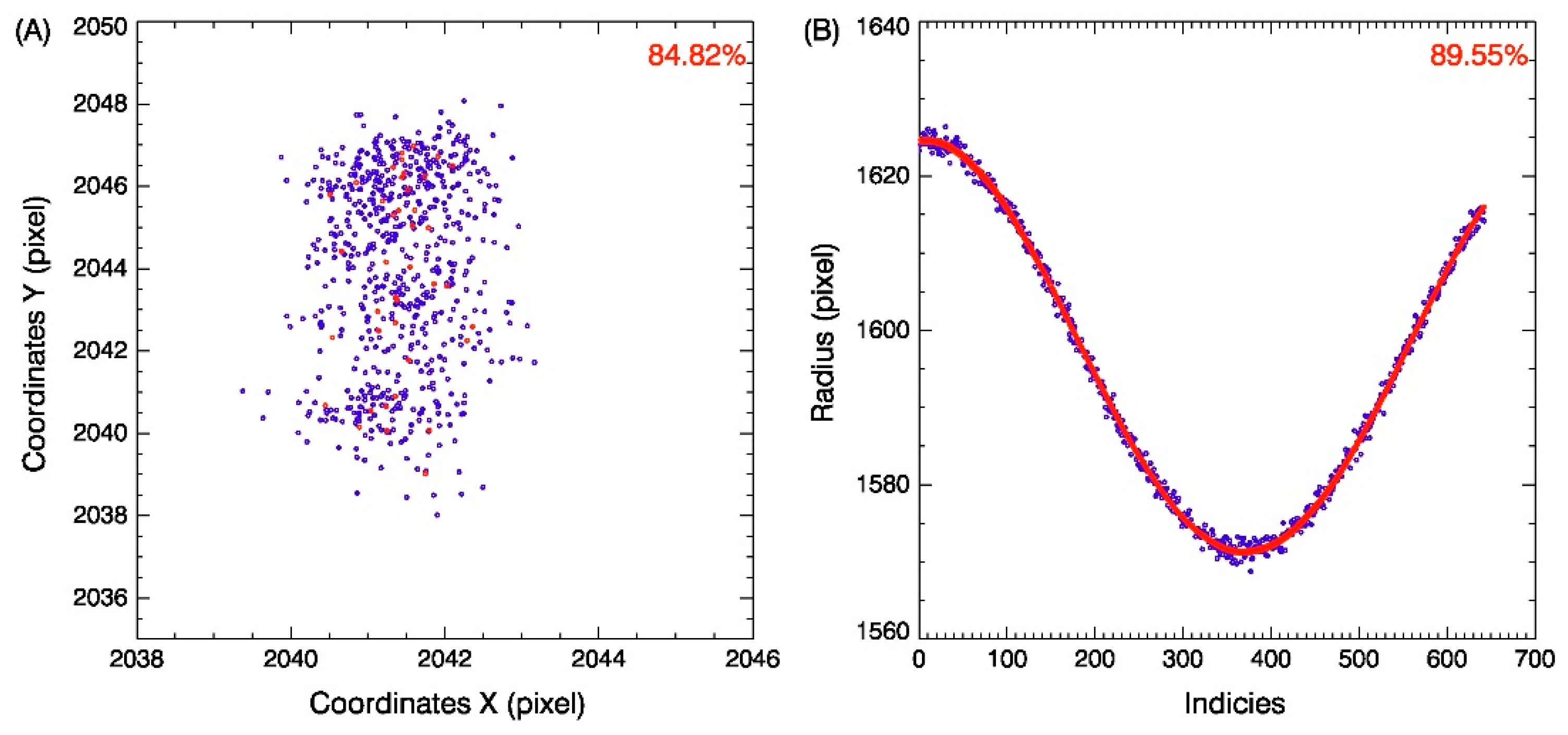
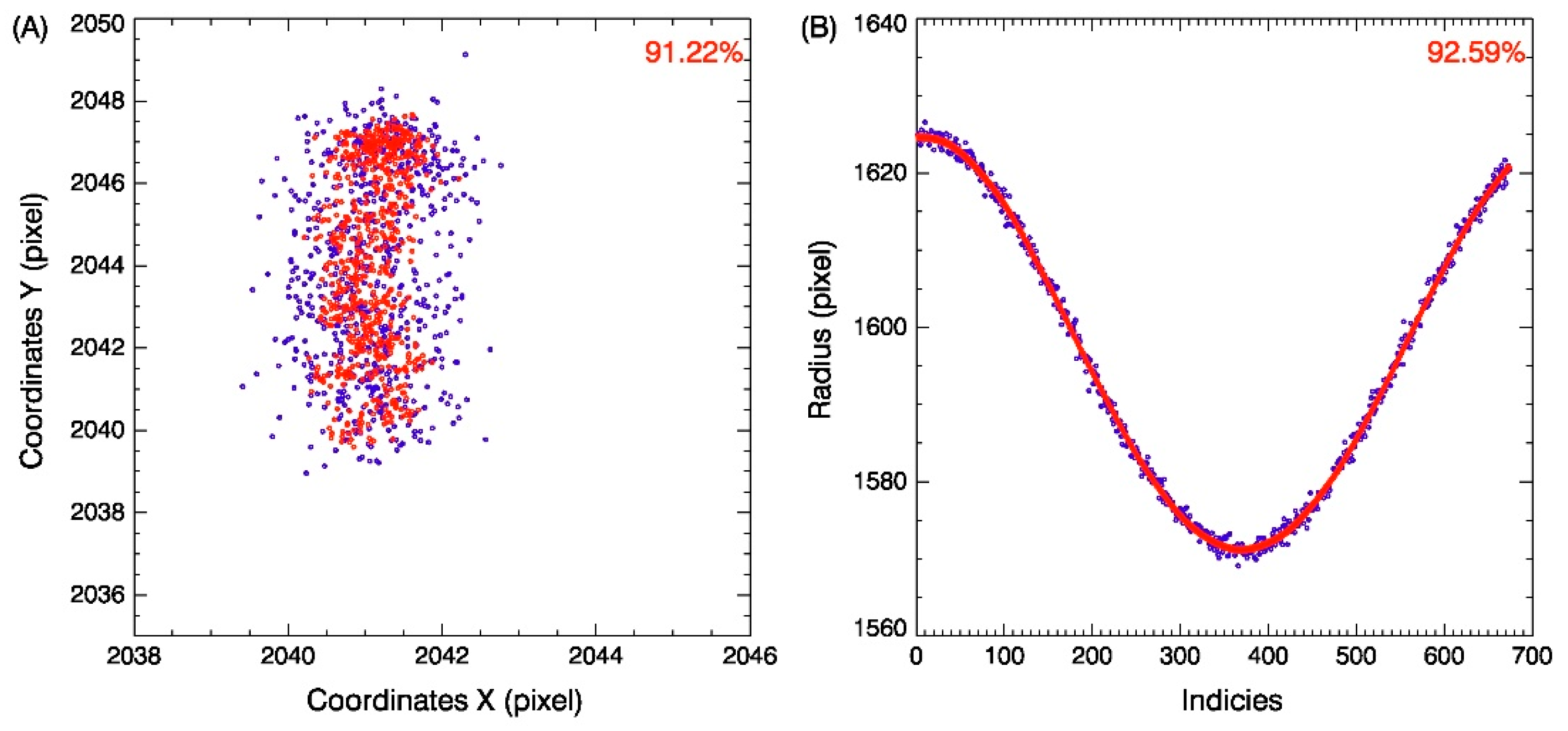
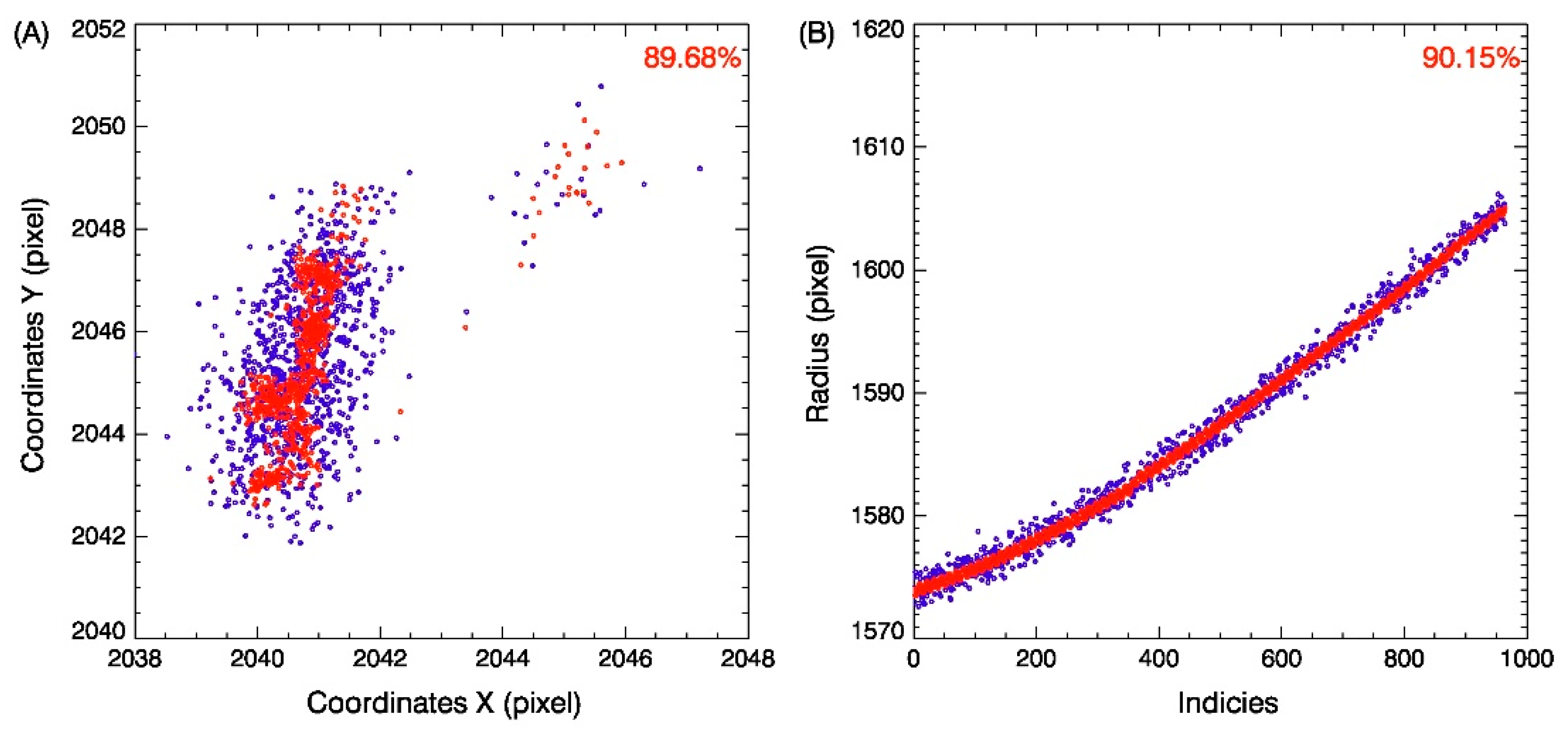
To verify the effectiveness of the proposed algorithm and its applicability under different solar activities, the solar 19.5 nm images from three years were selected for statistical comparison analysis. There were 718 images with a time interval of 12 h in all of 2014, 729 images with a time interval of 12 h in all of 2019, and 1076 solar images from 1 August 2021 to 31 October 2021. The sun in 2014 was more active, while in 2019, it reached a minimum, and between August and October 2021, the solar activity was moderate. The solar disk centers and boundaries calculated by the proposed method were compared with the results released by the AIA team. The comparison results, given in Table 1, were classified according to four constraints with |Xcalculation − XAIA| ≤ 2 pixels and |Ycalculation − YAIA| ≤ 2 pixels, |Xcalculation − XAIA| > 2 pixels or |Ycalculation − YAIA| > 2 pixels, |Rcalculation − RAIA| ≤ 3 pixels, and |Rcalculation − RAIA| > 3 pixels. From Table 1, we can conclude that the algorithm performs better during smaller solar activity than when the sun is more active. It is to be expected cause the solar boundary will be clearer after FLICM and background removal processes. The scatter charts for statistical comparison under the conditions of |Xcalculation − XAIA| ≤ 2 pixels and |Ycalculation − YAIA| ≤ 2 pixels, and |Rcalculation − RAIA| ≤ 3 pixels are given in Figure 7, Figure 8 and Figure 9. The image data in Figure 7 was from 2014, and the data in Figure 8 and Figure 9 were obtained in 2019 and 1 August 2021 to 31 October 2021, respectively. The blue points in each panel are the calculation of the proposed algorithm, and the red points are the results of AIA. The ratios are marked in red font at the upper right corners. A are the comparisons of solar center coordinates, and B are the comparisons of solar radii in each figure.
7. Conclusions
In this paper, an algorithm to extract the boundary and center of EUV solar image using the FLICM algorithm and Sobel operator was proposed. Based on the solar EUV images observed by SDO/AIA, the extraction results and accuracy were given and discussed. Using the Sobel operator, the image boundary can be found preliminarily, and the boundary image was further clustered by the FLICM algorithm. After the FLICM operation, the useful data points and the noise are further separated, and finally, the boundary points are determined using the least square circle fitting. The statistical comparison results of 1076 images from 1 August 2021 to 31 October 2021, 718 images in all of 2014, and 729 images in all of 2019 demonstrate that the algorithm is accurate and effective. The processes of the algorithm are summarized as follows:
- (1)
- Calculating the preliminary boundary using the Sobel operator;
- (2)
- Clustering the preliminary boundary image with the FLICM algorithm and the image is clustered into 10 categories;
- (3)
- The background is generally removed based on the clustered image; the 5 categories with the smaller values are considered the background;
- (4)
- Searching the peak value points from outside to inside around the image;
- (5)
- Fitting these points as the final boundary circle using the least square circle fitting method.
Author Contributions
Conceptualization, S.L. and B.L.; methodology, S.L. and J.Z.; software, S.L.; validation, J.Z., B.L. and C.J.; formal analysis, S.L.; investigation, S.L., C.J. and Y.S.; resources, B.L.; data curation, L.R. and J.X.; writing—original draft preparation, S.L.; writing—review and editing, S.L.; visualization, S.L.; supervision, B.L.; project administration, J.Z.; funding acquisition, J.X. All authors have read and agreed to the published version of the manuscript.
Funding
This work was supported by the First Class Fund for Distinguished Young Scholars of the Xi’an Branch of China Academy of Space Technology (Y21-RCFYJQ1-09).
Institutional Review Board Statement
Not applicable.
Informed Consent Statement
Not applicable.
Data Availability Statement
The solar data used in this paper are available at https://sdac.virtualsolar.org/cgi/search.
Conflicts of Interest
The authors declare no conflict of interest.
References
- Domingo, V.; Fleck, B.; Poland, A.I. SOHO: The Solar and Heliospheric Observatory. Space Sci. Rev. 1995, 72, 81–84. [Google Scholar] [CrossRef]
- Martens, P.; Muglach, K. Scientific Highlights from the Solar and Heliospheric Observatory. In Solar Polarization; Springer: Dordrecht, The Netherlands, 1999. [Google Scholar]
- Delaboudinière, J.P.; Artzner, G.E.; Brunaud, J.; Gabriel, A.H.; Hochedez, J.F.; Millier, F.; Song, X.Y.; Au, B.; Dere, K.P.; Howard, R.A.; et al. EIT: Extreme-ultraviolet Imaging Telescope for the SOHO mission. Sol. Phys. 1995, 162, 291–312. [Google Scholar] [CrossRef]
- Strong, K.; Bruner, M.; Tarbell, T.; Wolfson, C.J. Trace—The transition region and coronal explorer. Space Sci. Rev. 1994, 70, 119–122. [Google Scholar] [CrossRef]
- Handy, B.; Bruner, M.; Tarbell, T.; Title, A.; Wolfson, C.; LaForge, M.; Oliver, J. UV Observations with the Transition Region and Coronal Explorer. Sol. Phys. 1998, 183, 29–43. [Google Scholar] [CrossRef]
- Cheimets, P.; Caldwell, D.C.; Chou, C.; Gates, R.; Lemen, J.; Podgorski, W.A.; Wolfson, C.J.; Wuelser, J.P. SDO-AIA telescope design. In Proceedings of the SPIE Optical Engineering + Applications, San Diego, CA, USA, 2–6 August 2009; Volume 7438, p. 74380G. [Google Scholar]
- Lemen, J.R.; Akin, D.J.; Boerner, P.F.; Chou, C.; Drake, J.F.; Duncan, D.W.; Edwards, C.G.; Friedlaender, F.M.; Heyman, G.F.; Hurlburt, N.E.; et al. The Atmospheric Imaging Assembly (AIA) on the Solar Dynamics Observatory (SDO). In The Solar Dynamics Observatory; Springer: New York, NY, USA, 2011. [Google Scholar]
- Marsch, E.; Fleck, B.; Schwenn, R. Solar Orbiter—A High Resolution Mission to the Sun and Inner Helisophere. COSPAR Colloq. Ser. 2001, 11, 445. [Google Scholar]
- Rochus, P.; Auchère, F.; Berghmans, D.; Harra, L.; Schmutz, W.; Schühle, U.; Addison, P.; Appourchaux, T.; Cuadrado, R.A.; Baker, D.; et al. The Solar Orbiter EUI instrument: The Extreme Ultraviolet Imager. Astron. Astrophys. 2020, 642, A8. [Google Scholar] [CrossRef]
- Chen, B.; Ding, G.-X.; He, L.-P. Solar X-ray and Extreme Ultraviolet Imager (X-EUVI) loaded onto China’s Fengyun-3E Satellite. Light. Sci. Appl. 2022, 11, 29. [Google Scholar] [CrossRef] [PubMed]
- Shimizu, T.; Katsukawa, Y.; Matsuzaki, K.; Ichimoto, K.; Kano, R.; DeLuca, E.E.; Lundquist, L.L.; Weber, M.; Tarbell, T.D.; Shine, R.A.; et al. Hinode Calibration for Precise Image Co-alignment between SOT and XRT (November 2006–April 2007). Publ. Astron. Soc. Jpn. 2007, 59 (Suppl. S3), S845–S852. [Google Scholar] [CrossRef] [Green Version]
- Couvidat, S.; Schou, J.; Hoeksema, J.T.; Bogart, R.S.; Bush, R.I.; Duvall, T.L.; Liu, Y.; Norton, A.A.; Scherrer, P.H. Observables Processing for the Helioseismic and Magnetic Imager Instrument on the Solar Dynamics Observatory. Sol. Phys. 2016, 291, 1887–1938. [Google Scholar] [CrossRef] [Green Version]
- Denker, C.; Johannesson, A.; Marquette, W.; Goode, P.R.; Wang, H.; Zirin, H. Synoptic Hα Full-Disk Observations of the Sun from Big Bear Solar Observatory—I. Instrumentation, Image Processing, Data Products, and First Results. Sol. Phys. 1999, 184, 87–102. [Google Scholar] [CrossRef]
- Wang, Y.; Liu, S.; Deng, Y.; Bai, X.; Mao, X. The measurement of flat fields and polarization offset from the routine observation data of a solar rotation. Chin. Sci. Bull. 2017, 63, 301–310. [Google Scholar] [CrossRef]
- Wang, Y.; Bai, X.; Liu, S.; Deng, Y.; SUN, Y. Flat-field measuring and correction method for full-disk solar image based on ground glass. Chin. Sci. Bull. 2017, 62, 3057–3066. [Google Scholar] [CrossRef]
- Wang, Y.; Bai, X.; Liu, S.; Deng, Y.; Zhang, Z.; Sun, Y. Flat-fielding of Full-disk Solar Images with a Gaussian-type Diffuser. Sol. Phys. 2019, 294, 127. [Google Scholar] [CrossRef]
- Shine, R.A.; Nightingale, R.W.; Boerner, P.; Tarbell, T.D.; Wolfson, C.J. Flat Fielding and Image Alignments for AIA/SDO Data Images. In Proceedings of the AGU Meeting, San Francisco, CA, USA, 13–17 December 2010; p. SH23C-1872. [Google Scholar]
- Shine, R.A.; Wolfson, C.; Boerner, P.F.; Tarbell, T.D.; Nightingale, R.W. Monitoring Image Alignments and Flat Fields for AIA/SDO Data Images. In Proceedings of the SPD Meeting #42, Las Cruces, NM, USA, 12–16 June 2011; pp. 21–26. [Google Scholar]
- Zhang, J.Y.; Yan, C.; Huang, X.X. Edge detection of images based on improved Sobel operator and genetic algorithms. In Proceedings of the 2009 International Conference on Image Analysis and Signal Processing, Linhai, China, 11–12 April 2009. [Google Scholar]
- Kanopoulos, N.; Vasanthavada, N.; Baker, R. Design of an image edge detection filter using the Sobel operator. IEEE J. Solid-State Circuits 1988, 23, 358–367. [Google Scholar] [CrossRef]
- Krinidis, S.; Chatzis, V. A Robust Fuzzy Local Information C-Means Clustering Algorithm. IEEE Trans. Image Process. 2010, 19, 1328–1337. [Google Scholar] [CrossRef] [PubMed]
- Ding, G.; He, F.; Zhang, X.; Chen, B. A new auroral boundary determination algorithm based on observations from TIMED/GUVI and DMSP/SSUSI. J. Geophys. Res. Space Phys. 2017, 122, 2162–2173. [Google Scholar] [CrossRef]
- Liu, F.; Han, P.; Wei, Y.; Yang, K.; Huang, S.; Li, X.; Zhang, G.; Bai, L.; Shao, X. Deeply seeing through highly turbid water by active polarization imaging. Opt. Lett. 2018, 43, 4903–4906. [Google Scholar] [CrossRef] [PubMed]
- Liu, F.; Wei, Y.; Han, P.; Yang, K.; Bai, L.; Shao, X. Polarization-based exploration for clear underwater vision in natural illumination. Opt. Express 2019, 27, 3629–3641. [Google Scholar] [CrossRef] [PubMed]
- Liu, F.; Zhang, S.; Han, P.; Chen, F.; Zhao, L.; Fan, Y.; Shao, X. Depolarization index from Mueller matrix descatters imaging in turbid water. Chin. Opt. Lett. 2022, 20, 022601. [Google Scholar] [CrossRef]
Figure 1.
(A) is the 19.3 nm solar image observed by AIA at 09:39:40 UTC on 28 August 2021, and (B) is the local enlarged image in the rectangular box in A. The observation time is marked in the lower left corner of A.
Figure 1.
(A) is the 19.3 nm solar image observed by AIA at 09:39:40 UTC on 28 August 2021, and (B) is the local enlarged image in the rectangular box in A. The observation time is marked in the lower left corner of A.

Figure 2.
The original solar image (A) and the image calculated by Sobel operator (B).

Figure 3.
The images calculated by Sobel operator (A), the image calculated by FLICM algorithm (B), and the image after background removal (C–F) are the partially enlarged views corresponding to (A–C).
Figure 3.
The images calculated by Sobel operator (A), the image calculated by FLICM algorithm (B), and the image after background removal (C–F) are the partially enlarged views corresponding to (A–C).

Figure 4.
The normalized gray values vs. pixels along the lines in Figure 3D (green) and Figure 3F (blue). The red dotted line represents the boundary along the line.

Figure 5.
The fitted circle boundary using the least square circle fitting (A,B) is a partially enlarged view of (A,C) the fitted boundary in the original solar EUV image.
Figure 5.
The fitted circle boundary using the least square circle fitting (A,B) is a partially enlarged view of (A,C) the fitted boundary in the original solar EUV image.

Figure 6.
The calculated boundaries of the solar 19.3 nm (A), 17.1 nm (B), and 13.1 nm (C) images observed by AIA using the proposed method. The observation time is marked in the lower left corner of each image.
Figure 6.
The calculated boundaries of the solar 19.3 nm (A), 17.1 nm (B), and 13.1 nm (C) images observed by AIA using the proposed method. The observation time is marked in the lower left corner of each image.

Figure 7.
The image data was obtained in 2014, and the sun was more active. (A) is the comparison of the 609 samples of solar centers between our calculations (blue points) and the results of AIA (red points), and (B) is the comparison of the 643 samples of solar radii between our calculations (blue points) and the results of AIA (red points).

Figure 8.
The image data was obtained in 2019, and the solar activity was minimum. (A) is the comparison of the 665 samples of solar centers between our calculations (blue points) and the results of AIA (red points), and (B) is the comparison of the 675 samples of solar radii between our calculations (blue points) and the results of AIA (red points).

Figure 9.
The image data was obtained from 1 August 2021 to 31 October 2021, and the solar activity was moderate. (A) is the comparison of the 965 samples of solar centers between our calculations (blue points) and the results of AIA (red points), and (B) is the comparison of the 970 samples of solar radii between our calculations (blue points) and the results of AIA (red points).


Table 1.
Statistical comparison of the calculated solar centers and radii with the results of AIA.
| Date | 2014 | 2019 | 2021 |
|---|---|---|---|
| Solar level | active | quiet | moderate |
| Total images | 718 | 729 | 1076 |
| |Xcalculation − XAIA| ≤ 2 pixels and |Ycalculation − YAIA| ≤ 2 pixels | 609 (84.82%) | 665 (91.22%) | 965 (89.68%) |
| |Xcalculation − XAIA| > 2 pixels or |Ycalculation − YAIA| > 2 pixels | 109 (15.18%) | 64 (8.78%) | 111 (10.32%) |
| |Rcalculation − RAIA| ≤ 3 pixels | 643 (89.55%) | 675 (92.59%) | 970 (90.15%) |
| |Rcalculation − RAIA| > 3 pixels | 75 (10.45%) | 54 (7.41%) | 106 (9.85%) |
Publisher’s Note: MDPI stays neutral with regard to jurisdictional claims in published maps and institutional affiliations. |
© 2022 by the authors. Licensee MDPI, Basel, Switzerland. This article is an open access article distributed under the terms and conditions of the Creative Commons Attribution (CC BY) license (https://creativecommons.org/licenses/by/4.0/).
Share and Cite
MDPI and ACS Style
Li, S.; Zhang, J.; Liu, B.; Jiang, C.; Ren, L.; Xue, J.; Song, Y. An Algorithm to Extract the Boundary and Center of EUV Solar Image Based on Sobel Operator and FLICM. Photonics 2022, 9, 889. https://doi.org/10.3390/photonics9120889
AMA Style
Li S, Zhang J, Liu B, Jiang C, Ren L, Xue J, Song Y. An Algorithm to Extract the Boundary and Center of EUV Solar Image Based on Sobel Operator and FLICM. Photonics. 2022; 9(12):889. https://doi.org/10.3390/photonics9120889
Chicago/Turabian StyleLi, Shuai, Jianhua Zhang, Bei Liu, Chengzhi Jiang, Lanxu Ren, Jingjing Xue, and Yansong Song. 2022. "An Algorithm to Extract the Boundary and Center of EUV Solar Image Based on Sobel Operator and FLICM" Photonics 9, no. 12: 889. https://doi.org/10.3390/photonics9120889
Note that from the first issue of 2016, this journal uses article numbers instead of page numbers. See further details here.