An Improved Analytical Model of a Spectrometer for Optical Coherence Tomography

Abstract

We present an improved analytical model of a spectrometer for optical coherence tomography (OCT), which more accurately describes the OCT in-depth sensitivity fall-off. The model considers the intrinsic spectral resolution of the dispersive element and the influence of additional components (inequidistance-correcting prism). The model is validated by experimental data obtained both from other studies and our own experiments. The influence of the frequency response of the CCD electrical circuit and the analog-to-digital converter to the OCT signal fall-off was also detected and was shown to be significant in some cases.

1. Introduction

Optical coherence tomography (OCT) is an interferometric imaging technique of scattering structure of optically turbid media, especially biological tissues. OCT is mostly used for non-invasive imaging of biological structures for clinical diagnostics. One of the widespread varieties of OCT is a spectral-domain type (SD-OCT), which is based on an optical spectrometer [1].

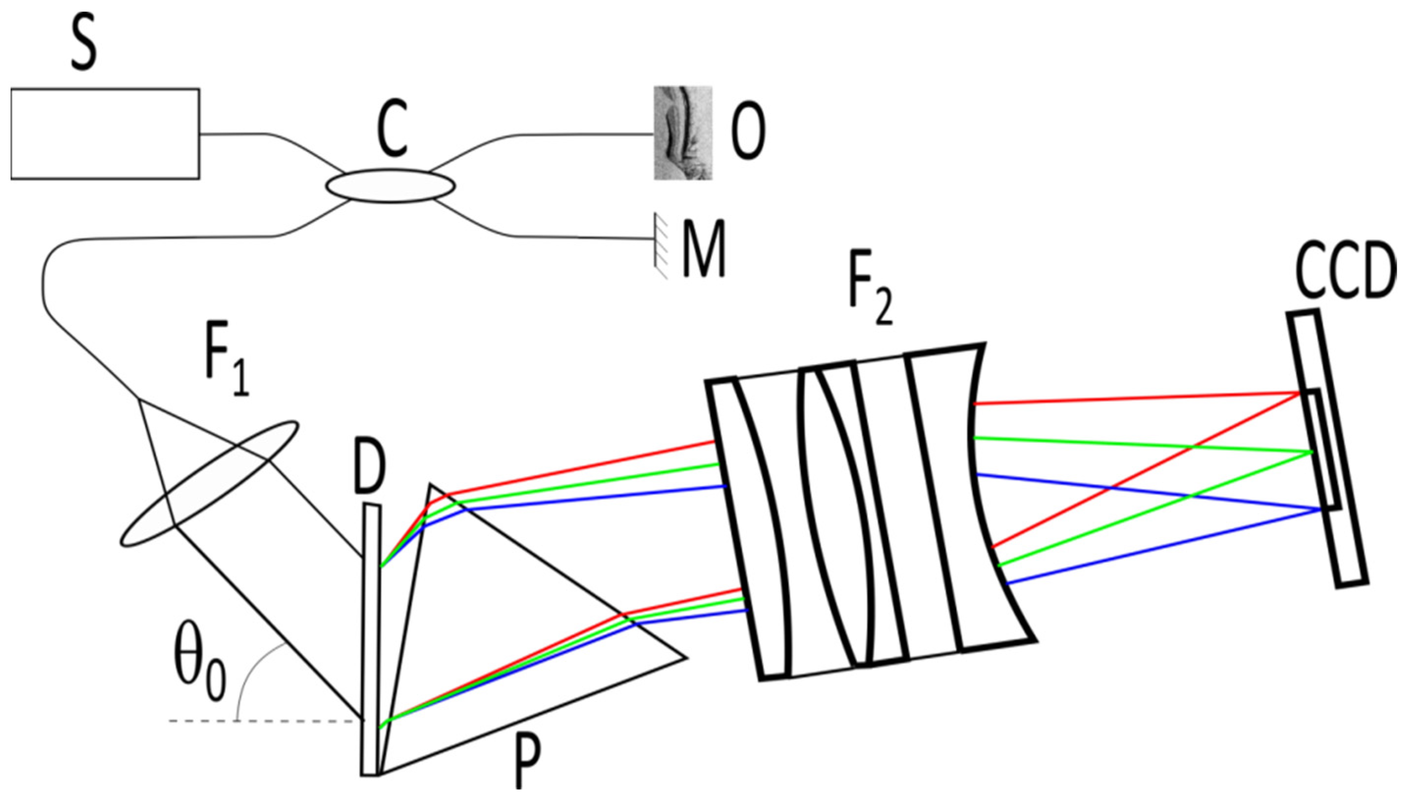
An OCT signal is formed by recording and further processing the interference of two light beams—a reference beam and a beam scattered by the object. Initial beams are formed from light source S using an optical splitter C (Figure 1). The reference beam is formed upon reflection from the reference plane M, the scattered beam—as a result of the scattering of the probe beam on optical inhomogeneities of the medium under study O. The radiation scattered by the medium is directed back to the optical splitter, where it is added to the reference radiation and then sent to the recording system, which in spectral-domain OCT consists of a spectrometer built on a diffraction grating D and a matrix photodetector (commonly a linear CCD array). The interference of the reference and scattered light provides a modulation of the optical spectrum in k-space. Each spatial frequency of the modulation is associated with the in-depth position of the scatterer by the Fourier transform.

The use of spectral sampling of the OCT signal has both strengths (a significant increase in speed compared to correlation methods [2]) and weaknesses, which consists of the appearance of additional unwanted image elements (autocorrelation and mirror artifacts [3,4,5,6]), a vulnerability in relation to the Doppler frequency shift arising from the probe-to-object relative movement while in vivo imaging [7,8], and a decrease in the level of useful signal with an increase in the interfering waves optical path difference [9]. The latter manifests itself regardless of the features of radiation scattering in the object medium and the position of the focusing plane or the sharpness of the probing beam. This effect is known as sensitivity fall-off and is usually associated with finite sizes of both detecting pixels in the CCD array and point spread function (PSF) of the spectrometer focusing lens [9,10,11,12]. These factors decrease the amplitude of interference-caused spectrum modulation (i.e., OCT signal level) with an increase of modulation frequency corresponded to optical path length difference (i.e., the in-depth position of the observation point). Thus, the OCT signal becomes weaker in depth.

There have been several attempts to overcome the sensitivity fall-off influence. Here, we should note the development of the complex OCT approach [3,5,13] and Talbot-fringes OCT [14,15]. The first technique introduces phase modulation between reference and probing waves for a series of consecutive A-scans, therefore, the OCT signal becomes sensitive to the sign of the path difference. It allows shifting zero-delay surface to some depth under the tissue surface, decreasing the signal level from the surface and preserving it at the said depth. Talbot-fringes OCT operates with two parallel-shifted beams in a spectrometer. This setup causes additional modulation along the spectrum image in a spectrometer (Talbot-fringes), therefore, the interference-caused modulation is heterodyned by the Talbot-fringes frequency. This approach allows decreasing interference-caused spectrum modulation frequency corresponded for deeper scatterers and, thus, increasing OCT signal level.

For qualitative estimation of sensitivity fall-off FO, the following formula was proposed and used in OCT developments [10,12,16]:

$$FO\left(z\right)=\frac{\sin \left(p{R}_{0}z\right)}{p{R}_{0}z}\ast \exp \left[-\frac{a^2{R}_0{}^2{z}^2}{4\ln 2}\right],$$

(1)

where z is the imaging depth, p is the width of a single CCD pixel, R₀ denotes the mutual linear dispersion in a spectrometer (spectral width in k corresponding to 1 μm in CCD plane), a is the optical beam width. Equation (1) claims to be a complete description of spectrometer-caused in-depth sensitivity fall-off in OCT images. However, experimental results [12] show sensitivity fall-off to be significantly higher than predicted by Equation (1). It enforces developers to seek other possibilities and generate conclusions on used optics imperfection [12]. The last does not seem quite realistic, especially since the calculation omitted an important element—the effect of the own resolution of the spectrometer’s dispersive element.

This study aims at formulating a refined description of an SD-OCT in-depth sensitivity, taking into account the effect of the resolution of the diffractive grating and combined dispersive element, comprising the grating and optical prism.

2. Materials and Methods

The optical intensity spectrum of the sum of two interfering waves with the delay of Δz is modulated in k-space by a sinus-like waveform with the frequency proportional to said Δz, and the amplitude is determined by the product of the wave intensities. The tissue under OCT imaging may be described as a set of scatterers characterized by some distribution in tissue space and scattering properties. Each scattered light portion contributes to the formation of the overall spectrum modulation. Hereinafter, we suppose that any autocorrelation artifacts [5] are eliminated from the signal and we consider only those components resulting from interference between reference and backscattered waves. The localization of scatterers along the depth-axis (z) and the value of backscattered light—so-called A-scan FA(z)—are reconstructed by Fourier transformation of optical intensity spectrum S(k) recorded in the spectrometer.

$$FA\left(z\right)=ℱ\left(S\left(k\right)\right)\left(\mathrm{z}\right),$$

(2)

Equation (2) also describes the envelope of the value of the reconstructed signal from a single scatterer placed at different depths along the probing beam. This envelope describes sensitivity at each depth and could be found in Equation (2) by substituting S(k) with the shape of single resolved spectral component fA(k). fA(k) is determined by the convolution [11,17] of three functions recorded in k-space:

$$fA\left(k\right)=PSF\left(k\right)\otimes SW\left(k\right)\otimes DG\left(k\right)$$

(3)

where PSF(k) is a point spread function of focusing beam determined only by the focusing lens and beam diameter and converted in k-space using the spectrometer dispersion formula; SW(k) is the k-space-converted image of rectangular sensitivity shape of a single element of the CCD array; DG(k) is the diffractive grating resolution function. In contradistinction to previous models, we take into account the exact shape of DG(k). This function describes the angular dependence of light intensity for monochromatic components diffracting on the grating by converting into k-space.

Since the envelope of the reconstructed signal FE(z) value represents a Fourier image of fA(k), it is the product of the three Fourier images of functions listed previously:

$$FE\left(z\right)=ℱ\left(PSF\right)\left(\mathrm{z}\right)·ℱ\left(SW\right)\left(\mathrm{z}\right)·ℱ\left(DG\right)\left(\mathrm{z}\right)$$

(4)

This allows for considering their impacts separately.

2.1. Resolution of Diffractive Grating

Mostly, the diffractive grating resolution is estimated by the Rayleigh criterion and qualitatively is set as the ratio of the wavelength to the number of illuminated grating lines. For the OCT spectrometer description, it is common to ensure formal compliance of desirable spectral resolution to beam size on a grating. However, this approach has some weaknesses. First, the Rayleigh criterion is formulated for beams with a flat intensity shape and all scratches are to be illuminated by equal light. In real systems, the analyzed beam has a Gaussian shape, so peripheral scratches lead to low impact, in comparison to central ones. Second, the criterion expresses distinguishing between two adjacent peaks by eye, that is, the presence of an intensity dip between them at a magnitude of 80% of the peak value. This leads to a 5-fold decrease in spectrum modulation depth or, equivalently, a 5-fold decrease in the reconstructed signal value at the edge of the range.

For the OCT spectrometer, the most commonly used is the Bragg setup, in which the diffraction angle for the central component of the spectrum θ(k₀) is set equal to the angle of incidence of the optical beam light θ₀ on the grating with lines period d:

$$\sin \mathsf{\theta }\left(k_0\right)=\sin {\mathsf{\theta }}_0=\frac{\pi }{k_0·d}$$

(5)

This setup provides polarization independence and optimal diffraction efficacy to (−1) order if volume phase holographic grating (WasatchPhotonics) or other high density and precision gratings (LightSmyth product line from II-IV Max Levy, FSTG-NIR line from Ibsen Photonics) are used and allows for significant simplifying of analytical calculations. For the Bragg setup of the spectrometer, the envelope component in object depth-space $ℱ\left(DG\right)\left(\mathrm{z}\right)$is described by a Gaussian shape:

$$ℱ\left(DG\right)\left(\mathrm{z}\right)=e^{-\frac{z^2}{2{\delta }^2}},$$

(6)

where

$$\delta ={\sigma }_0\tan {\mathsf{\theta }}_0,$$

(7)

and σ₀ denotes the half-width of the optical beam after the spectrometer collimator F₁ and is determined by its focal length and fiber numerical aperture.

2.2. Dispersion in the Spectrometer

As mentioned above, PSF(k) and SW(k) initially are functions in image space that are converted in k-space using the spectrometer dispersion formula. Let R₀ be a reciprocal linear dispersion, indicating the width of the spectrum (in wavenumber) spread over 1 μm at the focal plane [12]. In general, the dependence between image space coordinates and wavenumbers is nonlinear and may be described by Taylor expansion as:

$$x\left(k\right)=x\left(k_0\right)+\frac{1}{R_0}·\left(k-k_0\right)+O\left(k-k_0\right)·{\left(k-k_0\right)}^2$$

(8)

However, for most spectrometers, analyzing the broadband light with a spectrum width up to 15% of the central frequency, the impact of the nonlinear component is less than 3–5% from the overall function range [18], even in the absence of a compensator prism that reduces this contribution to a value below tenths and hundredths of a percent [19,20]; therefore, the last term in Equation (8) may be omitted. For the Bragg configuration, the linear dispersion coefficient is found as:

$$\frac{1}{R_0}=\frac{dx}{dk}\left(k_0\right)=2F\tan \left({\mathsf{\theta }}_0\right)\frac{1}{k_0}$$

(9)

where F denotes the focal length of focusing lens F₂.

In contrast to swept-source OCT, where the equidistance of the received spectral components can be ensured through the implementation of frequency-dependent digitization [21,22,23,24], in the spectrometer-based OCT setup, to ensure equidistant optical frequency recording of spectral components, additional optical correctors may be used [12,18,19,20]. These provide some features to the device setup; firstly, a decrease in the number of calculations [20], however, this causes a significant (about 30%) decrease in the dispersion value 1/R₀ [18,19]. This decrease may be taken into account by the correction factor η defined for every spectrometer setup numerically. Taking into account this coefficient, the linear dispersion can be rewritten as the following:

$$\frac{1}{R}=2\mathsf{\eta }F\tan \left({\mathsf{\theta }}_0\right)\frac{1}{k_0}$$

(10)

2.3. Point-Spread Function in k-Space

The PSF(k) describes the optical limitations of focusing lens F₂. Ideally, the spot in the focal plane is described by Gaussian function with transversal size determined by focal length F, wavelength λ₀, and collimated beam size σ₀, much smaller than lens aperture:

$$∆x_0=\frac{{\lambda }_0}{\pi }\frac{F}{{\sigma }_0}$$

(11)

The corresponding envelope component in object depth-space $ℱ\left(PSF\right)\left(\mathrm{z}\right)$is also described by Gaussian shape

$$ℱ\left(PSF\right)\left(\mathrm{z}\right)=e^{-\frac{z^2}{2{\gamma }^2}},$$

(12)

where γ is found taking into account Equations (8) and (10) for the Bragg setup:

$$\gamma =\frac{1}{R·∆x_0}=\mathsf{\eta }·{\sigma }_0·\tan \left({\mathsf{\theta }}_0\right)$$

(13)

Since both components $ℱ\left(DG\right)\left(\mathrm{z}\right)$and $ℱ\left(PSF\right)\left(\mathrm{z}\right)$are Gaussian-shape functions, their joint impact may be formulated as a single Gaussian function:

$$ℱ\left(PSF\right)\left(\mathrm{z}\right)·ℱ\left(DG\right)\left(\mathrm{z}\right)=\exp \left[-\frac{z^2}{2z_G{}^2}\right],$$

(14)

where

$$z_G{}^2=\frac{{\mathsf{\eta }}^2}{1+{\mathsf{\eta }}^2}·\frac{1}{∆x_0{}^2{R}_0{}^2}$$

(15)

or

$$z_G{}^2=\frac{1}{1+{\mathsf{\eta }}^2}·\frac{1}{∆x_0{}^2{R}^2}$$

(16)

It is important to note that since the $ℱ\left(DG\right)\left(\mathrm{z}\right)$component has no dependence on the dispersion correction factor η, the influence of the corrector on the envelope cannot be taken into account by simply decreasing the dispersion value 1/R_0, or changing the focal length of focusing lens F₂. Thus, a spectrometer built using a prism-corrector has a fundamentally different description than a conventional spectrometer based on a single diffraction grating.

2.4. Spectrum Sampling Window

The third component in Equation (4) $ℱ\left(SW\right)\left(\mathrm{z}\right)$ is determined by the finite size of a single element of the CCD array. Its conversion to k-space is produced using the same linear dispersion coefficient (Equation (10)). If the pixel size is denoted as p (following [12,16]), then the envelope component is formulated as:

$$ℱ\left(SW\right)\left(\mathrm{z}\right)=\frac{\sin \left(pRz\right)}{pRz}$$

(17)

2.5. Signal Envelope

In accordance with Equation (4), the total expression for signal envelope in spectrometer-based OCT is given by:

$$FE\left(z\right)=\frac{\sin \left(pRz\right)}{pRz}·\exp \left[-\frac{\left(1+{\mathsf{\eta }}^2\right)}{2}·∆x_0{}^2{R}^2{z}^2\right]$$

(18)

In this case, the scales of the sinc and exponential components have significantly different dependencies from η, so the corrector prism influence cannot be accounted for changing the dispersion coefficient value.

2.6. Experimental Verification

The in-house SD-OCT device used for the experimental validation operates with a light source—λ₀ = 1055 nm. The spectrometer is based on grating with lines density 1/d = 1500 L/mm (T-1500-930 LightSmyth product line from II-IV Max Levy) and an equidistance correction 63.2 degrees prism made of K9 glass (Nanyang Jingliang optical technology corp, Nanyang city, China). The focal length of the focusing lens F₂ is 86 mm. The CCD array used for spectrum registration has a pixel width of 25 μm (Collins Aerospace SU512LD). The received spectrum width is 81 nm (corrector prism provides dispersion decreasing factor η = 0.74). The device operates under homemade software [25]—its electrical circuits are described in detail in [26].

The OCT signal was recorded from 4% reflecting surface placed into an optical beam with a Rayleigh length of 30 cm to overcome the influence of focusing nonuniformity during sample movement along the beam axis. This design—of the object simulation—is very important to exclude other factors causing in-depth sensitivity fall-off, such as focusing sharpness and the effect of scattering in the medium under study. These factors have greater variability depending on certain OCT setups and object properties and their consideration is beyond the scope of this article.

The envelope was calculated from OCT data recorded for several object positions with 150–300 μm gaps over 1.75 mm depth. Thus 15–20 object surface positions were recorded for a single envelope finding.

To highlight the influence of the frequency transfer characteristic of an electrical circuit on a signal envelope we increased the data rate 4-fold from 5000 spectra per second, recommended by the CCD array (SU512LD-1.7T1-0500) producer, to 20,000 spectra per second. This was achieved by increasing the main clock frequency, preserving both light power to be analyzed and its integration time to overcome changes to the signal-to-noise ratio [27].

Image reconstruction and analysis were carried out using in-house code on Python 4.2.

3. Results

3.1. Slow Image Acquisition

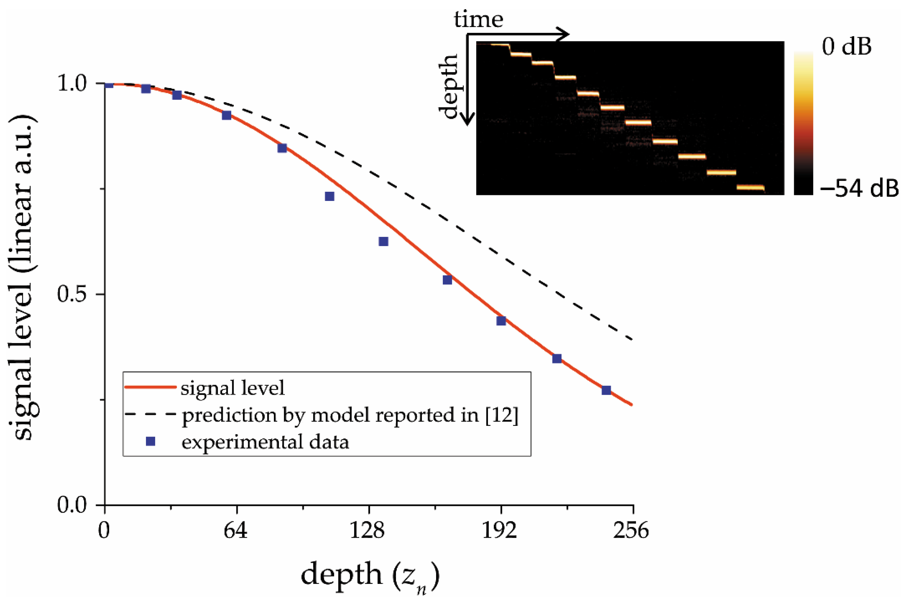
We recorded the value of the OCT signal for 11 different positions of surface in the probe arm of the interferometer (inset on Figure 2), preserving the total power of backscattered light. Averaged values of intensity at each surface stop were used to indicate signal level (dots on Figure 2). The depth scale is presented by 256 (corresponding to N = 512 photodetecting elements in the CCD array used in the experimental setup) dimensionless counts z_n given by

$$z_n=\frac{N}{2}\frac{z}{z_{max}},$$

(19)

where z is the current depth and z_max—maximal observing depth found by

$$z_{max}=\frac{{\lambda }_0^{2}N}{4∆\lambda }$$

(20)

In the current setup z_max value was 1.75 mm.

The presented points are in good correspondence with the prediction level given by Equation (18) which is presented by a red solid line on Figure 2. Conversely, the level presented on Figure 2 by a black dashed line predicted by a model from Equation (1), is noticeably higher at high depth. This indicates the materiality of the quantitative difference of the proposed description from the previous one and the sufficiency and reliability of the proposed analytical model of the spectrometer.

3.2. Fast Image Acquisition

The circuit transfer characteristics (the CCD electrical circuit and the analog-to-digital converter) may cause an additional sensitivity fall-off due to the transfer of the spatial frequency of modulation of the light intensity in the plane of the photodetector in the spectrometer into the temporal modulation of the signal, which is formed when the photocells are interrogated.

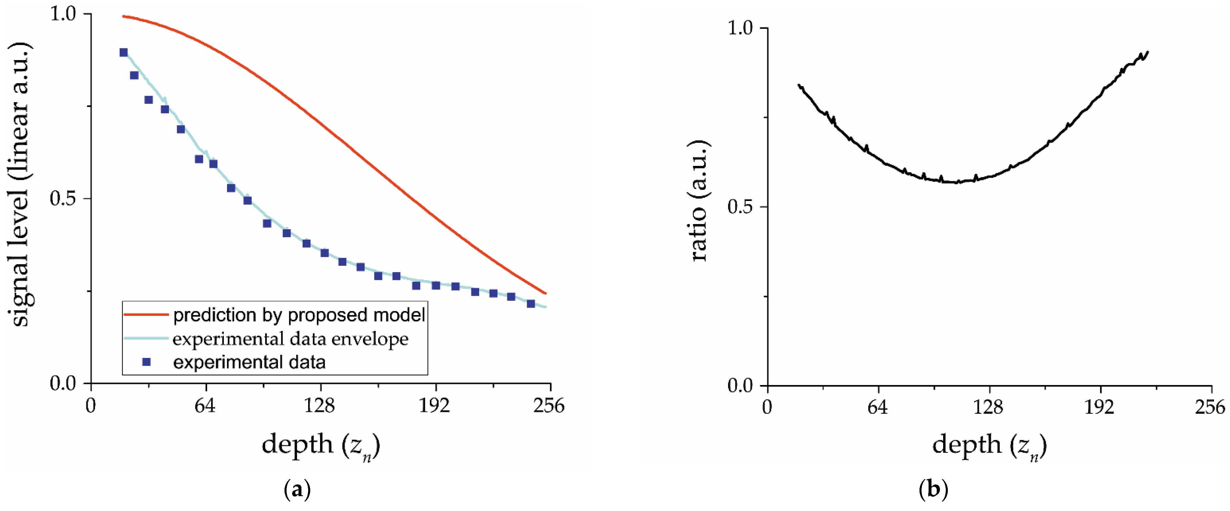
The results of the fast (four times faster than the producer’s recommendations) image acquisition experiment characteristics are demonstrated in Figure 3a. These results highlight the influence of the frequency transfer. In Figure 3a the obtained signal envelope (blue line, reconstructed from 24 different positions of surface in the probe arm of the interferometer, indicated as dots) is substantially omitted from the baseline. The quotient obtained by dividing the first by the second is presented in Figure 3b.

3.3. Other Reported OCT System Verification

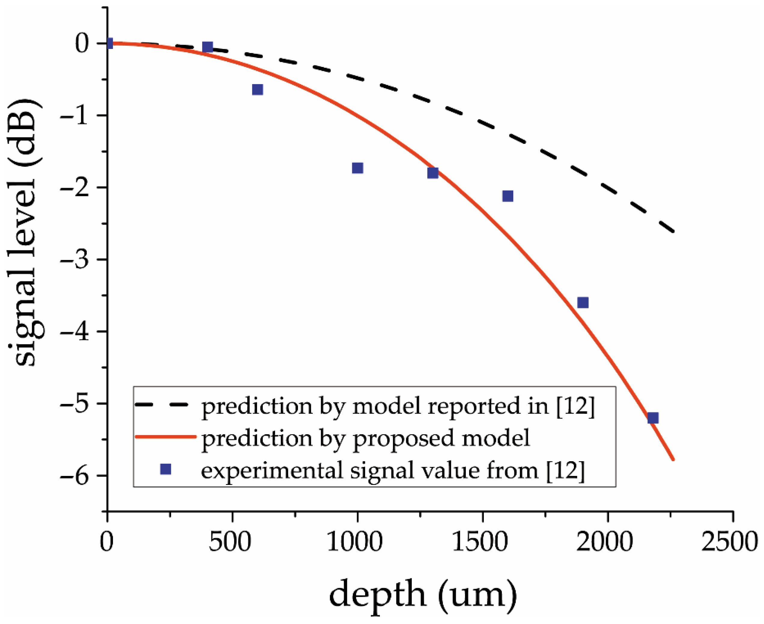
The improved analytical model also proved to be a good fit for experimental data published in [12]. We checked the proposed analytical model by experimental data provided in other studies. We extracted data points reported in [12], where authors wondered why their experimental results were not in agreement with the analytical model prediction, and compared them with our proposed model using the setup parameters given in [12]. The comparison result is shown in Figure 4.

4. Discussion

The proposed mathematical model of the OCT spectrometer takes into account two aspects omitted by earlier investigations. First, we considered the intrinsic spectral resolution of the dispersive element. A careful analysis shows that taking into account the factor of angular spectral resolution in the diffraction of light by a grating leads to a significant increase in the specific gravity of the exponential part in expression (1) with respect to sinc. However, this correction may be taken into consideration by correcting the effective beam width in this expression. Second, the influence of additional components—equidistance correcting prism—on the signal sensitivity fall-off in OCT was examined. It was shown that a spectrometer built using a prism-corrector had a fundamentally different description than a conventional spectrometer based on a single diffraction grating. In this case, the scales of the sinc and exponential components have significantly different dependencies from the dispersion decreasing factor η; therefore, the influence of the corrector prism cannot be accounted for as changing the dispersion coefficient value. In addition, it cannot be compensated by the corresponding increase in the focal length of the focusing lens in the spectrometer.

A closer look at the experimental data obtained in the validation experiment (Figure 2) reveals a slight deviation of the experimental data from the expected level in the central part of the image. This deviation may be insignificant, but it is a result of a four-factor decreasing signal level in spectrometer-based OCT. This factor is concerned with a frequency transfer characteristic of an electrical circuit between the CCD element and analog-to-digital converter, and the higher the electrical circuit time constant, the higher the deviation. This hypothesis was confirmed by the subsequent experiment, which consists of a four-fold increase in the carrier frequency of the radio signal coming from the CCD to the ADC. The reconstructed OCT data electrical circuit frequency characteristic profile is presented in Figure 3b. Its shape is symmetrical around the middle depth value, which also confirms the radio-technical nature of the observed signal deviation since the CCD element used in the setup has two separate output channels—one for odd and one for even pixels [28]. The researcher must be aware of the absence of the electrical circuit influence or consider it—especially when calculating the coefficients characterizing in depth the rate of attenuation of the OCT signal, depending on the type of tissue under study. This is important, because with such a substantial non-uniformity of the envelope, as shown in Figure 3b, the backscattering coefficient of biological tissue retrieved from OCT images can become dependent on the position of the analyzed area along the axis of the probing beam. The latter can be a potential source of diagnostic errors.

5. Conclusions

The mathematical model of the OCT spectrometer should take into account—in addition to the finite sizes of both detecting pixels in the CCD array and PSF of the focusing lens—the influence of the intrinsic spectral resolution of the dispersion element.

If the correction prism is used to minimize the inequidistance of recording spectral components in k-space, its influence on the spectrometer dispersion cannot be compensated by the use of a focusing lens with a corrected focal length, or taken into account by correcting only the dispersion formula.

The proposed improved spectrometer analytical model passed validation using experimental data obtained both from other studies and our own experiment. The validation demonstrates a very good correspondence between the experimental data and model predictions.

The influence of the frequency transfer characteristic of an electrical circuit between the CCD element and analog-to-digital converter was also detected and shown to be significant in some cases. Therefore, researchers must be aware of the absence of this influence, or consider it, especially when calculating the coefficients characterizing in depth the rate of attenuation of the OCT signal, depending on the type of tissue under study.

References

- Fercher, A.F. Optical coherence tomography. J. Biomed. Opt. 1996, 1, 157–173. [Google Scholar] [CrossRef] [PubMed]
- Choma, M.A.; Sarunic, M.V.; Yang, C.H.; Izatt, J.A. Sensitivity advantage of swept source and Fourier domain optical coherence tomography. Opt. Express 2003, 11, 2183–2189. [Google Scholar] [CrossRef] [PubMed] [Green Version]
- Targowski, P.; Wojtkowski, M.; Kowalczyk, A.; Bajraszewski, T.; Szkulmowski, M.; Gorczyńska, I. Complex spectral OCT in human eye imaging in vivo. Opt. Commun. 2004, 229, 79–84. [Google Scholar] [CrossRef]
- Wang, R.K.; Ma, Z. A practical approach to eliminate autocorrelation artefacts for volume-rate spectral domain optical coherence tomography. Phys. Med. Biol. 2006, 51, 3231–3239. [Google Scholar] [CrossRef] [PubMed]
- Leitgeb, R.A.; Wojtkowski, M. Optical Coherence Tomography: Techology and Applications; Fujimoto, J.G., Drexler, W., Eds.; Springer: Berlin/Heidelberg, Germany, 2008; pp. 177–207. [Google Scholar]
- Gelikonov, V.M.; Gelikonov, G.V.; Terpelov, D.A.; Shabanov, D.V.; Shilyagin, P.A. Suppression of image autocorrelation artefacts in spectral domain optical coherence tomography and multiwave digital holography. Quantum Electron. 2012, 42, 390. [Google Scholar] [CrossRef]
- Yang, G.-Z.; Hawkes, D.J.; Rueckert, D.; Noble, A.; Taylor, C. Medical Image Computing and Computer-Assisted Intervention—MICCAI 2009; Lecture Notes in Computer Science; Springer: Berlin/Heidelberg, Germany, 2009; Volume 5761, pp. 100–107. [Google Scholar]
- Ksenofontov, S.Y.; Shilyagin, P.A.; Terpelov, D.A.; Gelikonov, V.M.; Gelikonov, G.V. Numerical method for axial motion artifact correction in retinal spectral-domain optical coherence tomography. Front. Optoelectron. 2020, 13, 393–401. [Google Scholar] [CrossRef]
- Wang, K.; Ding, Z.; Chen, M.; Wang, C.; Wu, T.; Meng, J. Deconvolution with fall-off compensated axial point spread function in spectral domain optical coherence tomography. Opt. Commun. 2011, 284, 3173–3180. [Google Scholar] [CrossRef]
- Hu, Z.; Pan, Y.; Rollins, A.M. Analytical model of spectrometer-based two-beam spectral interferometry. Appl. Opt. 2007, 46, 8499–8505. [Google Scholar] [CrossRef]
- Shilyagin, P.A.; Gelikonov, G.V.; Gelikonov, V.M.; Shilyagina, N.Y. Over-depth artifacts elimination in spectral-domain optical coherence tomography. Proc. SPIE 2014, 8934, 83343H-1-8. [Google Scholar] [CrossRef]
- Lan, G.; Li, G. Design of a k-space spectrometer for ultra-broad waveband spectral domain optical coherence tomography. Sci. Rep. 2017, 7, 42353. [Google Scholar] [CrossRef]
- Gelikonov, V.M.; Kasatkina, I.V.; Shilyagin, P.A. Suppression of image artifacts in the spectral-domain optical coherence tomography. Radiophys. Quantum Electron. 2009, 52, 810–821. [Google Scholar] [CrossRef]
- Bradu, A.; Podoleanu, A.G. Attenuation of mirror image and enhancement of the signal-to-noise ratio in a Talbot bands optical coherence tomography system. J. Biomed. Opt. 2011, 16, 076010. [Google Scholar] [CrossRef] [Green Version]
- Woods, D.; Podoleanu, A. Controlling the shape of Talbot bands’ visibility. Opt. Express 2008, 16, 9654–9670. [Google Scholar] [CrossRef] [PubMed]
- Wang, L.; Yu, X.; Ge, X.; Wu, X.; Wang, X.; Bo, E.; Wang, N.; Liu, X.; Ni, G.; Liu, L. Design and optimization of a spectrometer for high-resolution SD-OCT. Laser Phys. Lett. 2019, 16, 045603. [Google Scholar] [CrossRef]
- Dorrer, C.; Belabas, N.; Likforman, J.-P.; Joffre, M. Spectral resolution and sampling issues in Fourier-transform spectral interferometry. J. Opt. Soc. Am. B 2000, 17, 1795–1802. [Google Scholar] [CrossRef]
- Gelikonov, V.M.; Gelikonov, G.V.; Shilyagin, P.A. Linear-wavenumber spectrometer for high-speed spectral-domain optical coherence tomography. Opt. Spectrosc. 2009, 106, 459–465. [Google Scholar] [CrossRef]
- Hu, Z.; Rollins, A.M. Fourier domain optical coherence tomography with a linear-in-wavenumber spectrometer. Opt. Lett. 2007, 32, 3525–3527. [Google Scholar] [CrossRef] [PubMed]
- Shilyagin, P.A.; Ksenofontov, S.; Moiseev, A.A.; Terpelov, D.A.; Matkivsky, V.A.; Kasatkina, I.V.; Mamaev, Y.A.; Gelikonov, G.V.; Gelikonov, V.M. Equidistant Recording of the Spectral Components in Ultra-Wideband Spectral-Domain Optical Coherence Tomography. Radiophys. Quantum Electron. 2018, 60, 769–778. [Google Scholar] [CrossRef]
- Choma, M.; Hsu, K.; Izatt, J. Swept source optical coherence tomography using an all-fiber 1300-nm ring laser source. J. Biomed. Opt. 2005, 10, 044009. [Google Scholar] [CrossRef]
- Jun, C.; Villiger, M.; Oh, W.-Y.; Bouma, B.E. All-fiber wavelength swept ring laser based on Fabry-Perot filter for optical frequency domain imaging. Opt. Express 2014, 22, 25805–25814. [Google Scholar] [CrossRef] [Green Version]
- Meleppat, R.K.; Matham, M.V.; Seah, L.K. An efficient phase analysis-based wavenumber linearization scheme for swept source optical coherence tomography systems. Laser Phys. Lett. 2015, 12, 055601. [Google Scholar] [CrossRef]
- Ratheesh, K.M.; Seah, L.K.; Murukeshan, V.M. Spectral phase-based automatic calibration scheme for swept source-based optical coherence tomography systems. Phys. Med. Biol. 2016, 61, 7652–7663. [Google Scholar] [CrossRef] [PubMed]
- Ksenofontov, S.Y. Application of the Method of Multiple Mutual Synchronization of Parallel Computational Threads in Spectral-Domain Optical Coherent Tomography Systems. Instrum. Exp. Tech. 2019, 62, 317–323. [Google Scholar] [CrossRef]
- Ksenofontov, S.Y.; Kupaev, A.V.; Vasilenkova, T.V.; Terpelov, D.A.; Shilyagin, P.A.; Moiseev, A.A.; Gelikonov, G.V. A High-Performance Data-Acquisition and Control Module Based on a USB 3.0 Interface for a NIR Broadband Spectrometer. Instrum. Exp. Tech. 2021, 64, 759–764. [Google Scholar] [CrossRef]
- Gelikonov, V.M.; Romashov, V.N.; Gelikonov, G.V. Excess broadband noise at equal intensities in the interferometer arms. Quantum Electron. 2021, 51, 377–382. [Google Scholar] [CrossRef]
- Ksenofontov, S.Y.; Terpelov, D.A.; Gelikonov, G.V.; Shilyagin, P.A.; Gelikonov, V.M. Elimination of Artifacts Caused by the Nonidentity of Parallel Signal-Reception Channels in Spectral Domain Optical Coherence Tomography. Radiophys. Quantum Electron. 2019, 62, 151–158. [Google Scholar] [CrossRef]
Figure 1.
Simplified OCT setup with spectrometer. S—low-coherent light source; C—coupler; M—reference mirror; O—object; F1, F2—collimating and focusing lenses; D—diffractive grating; P—correcting prism (optionally used to decrease the inequidistance of spectral components in optical frequency space); CCD—photodetector array.
Figure 2.
Signal obtained in experiment for several positions of object surface (blue dots, initial image presented on inset); theoretical prediction based on improved analytical model of spectrometer (red line) and prediction by model from Equation (1) (black dashes). Maximal depth of the image is 1.75 mm in air.
Figure 3.
(a) Sensitivity fall-off in OCT setup with significant influence of electrical circuit frequency characteristic; (b) characteristic profile obtained from recorded data as a ratio between experimental data envelope and signal level prediction.
Figure 4.
Signal obtained in the experiment reported in [12]; theoretical prediction based on previous model description (black dashes) and on improved analytical model of spectrometer (red).
Publisher’s Note: MDPI stays neutral with regard to jurisdictional claims in published maps and institutional affiliations. |
© 2021 by the authors. Licensee MDPI, Basel, Switzerland. This article is an open access article distributed under the terms and conditions of the Creative Commons Attribution (CC BY) license (https://creativecommons.org/licenses/by/4.0/).
Share and Cite
MDPI and ACS Style
Sherstnev, E.P.; Shilyagin, P.A.; Terpelov, D.A.; Gelikonov, V.M.; Gelikonov, G.V. An Improved Analytical Model of a Spectrometer for Optical Coherence Tomography. Photonics 2021, 8, 534. https://doi.org/10.3390/photonics8120534
AMA Style
Sherstnev EP, Shilyagin PA, Terpelov DA, Gelikonov VM, Gelikonov GV. An Improved Analytical Model of a Spectrometer for Optical Coherence Tomography. Photonics. 2021; 8(12):534. https://doi.org/10.3390/photonics8120534
Chicago/Turabian StyleSherstnev, Evgeny P., Pavel A. Shilyagin, Dmitry A. Terpelov, Valentin M. Gelikonov, and Grigory V. Gelikonov. 2021. "An Improved Analytical Model of a Spectrometer for Optical Coherence Tomography" Photonics 8, no. 12: 534. https://doi.org/10.3390/photonics8120534
Note that from the first issue of 2016, this journal uses article numbers instead of page numbers. See further details here.