Artificial Intelligence Based Methods for Asphaltenes Adsorption by Nanocomposites: Application of Group Method of Data Handling, Least Squares Support Vector Machine, and Artificial Neural Networks


 , and
, and
Abstract
:1. Introduction
2. Theory and Methods
2.1. Experimental Dataset
2.2. Models and Procedures
2.2.1. Least Squares Support Vector Machine (LSSVM)
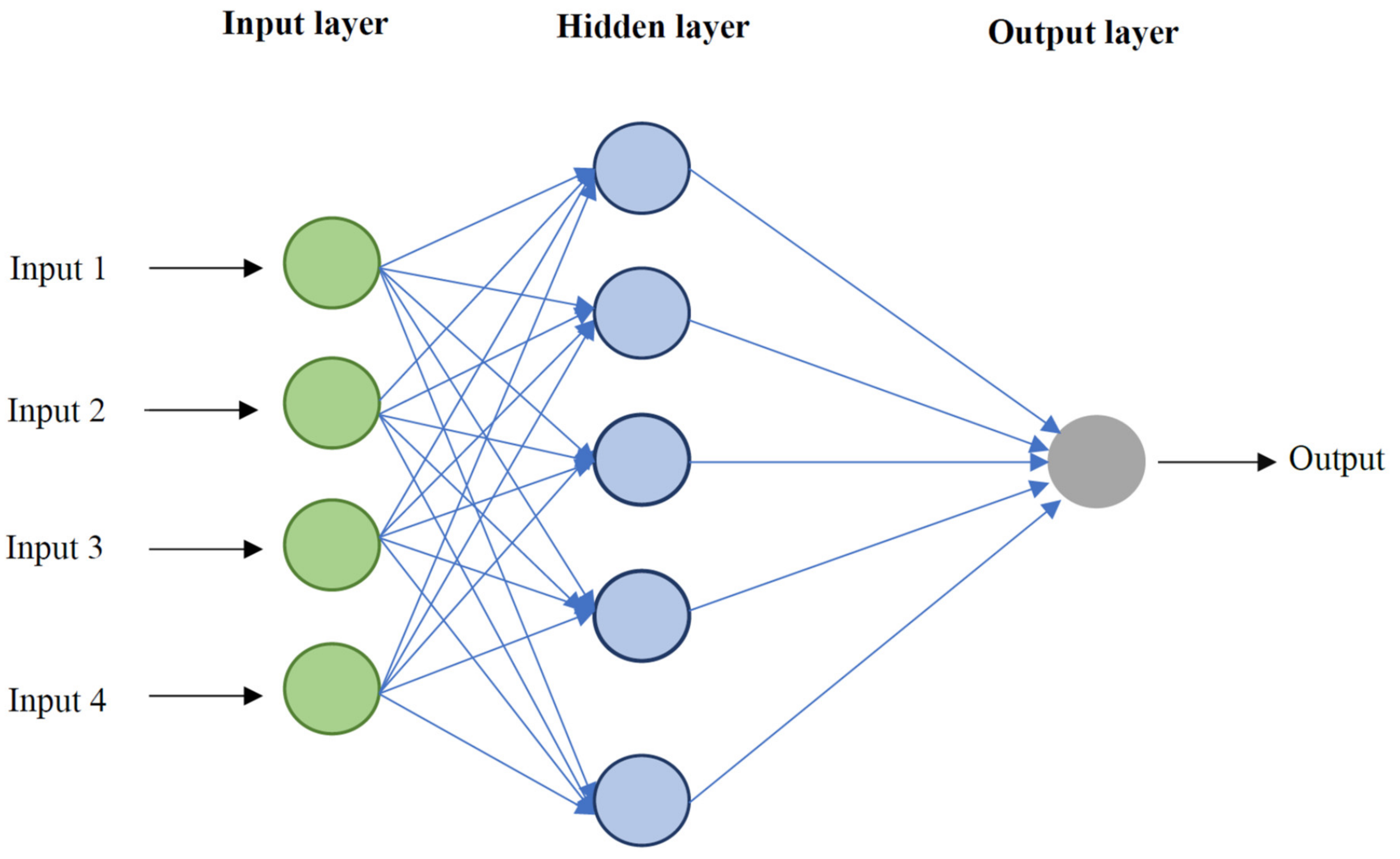
2.2.2. Artificial Neural Network (ANN)
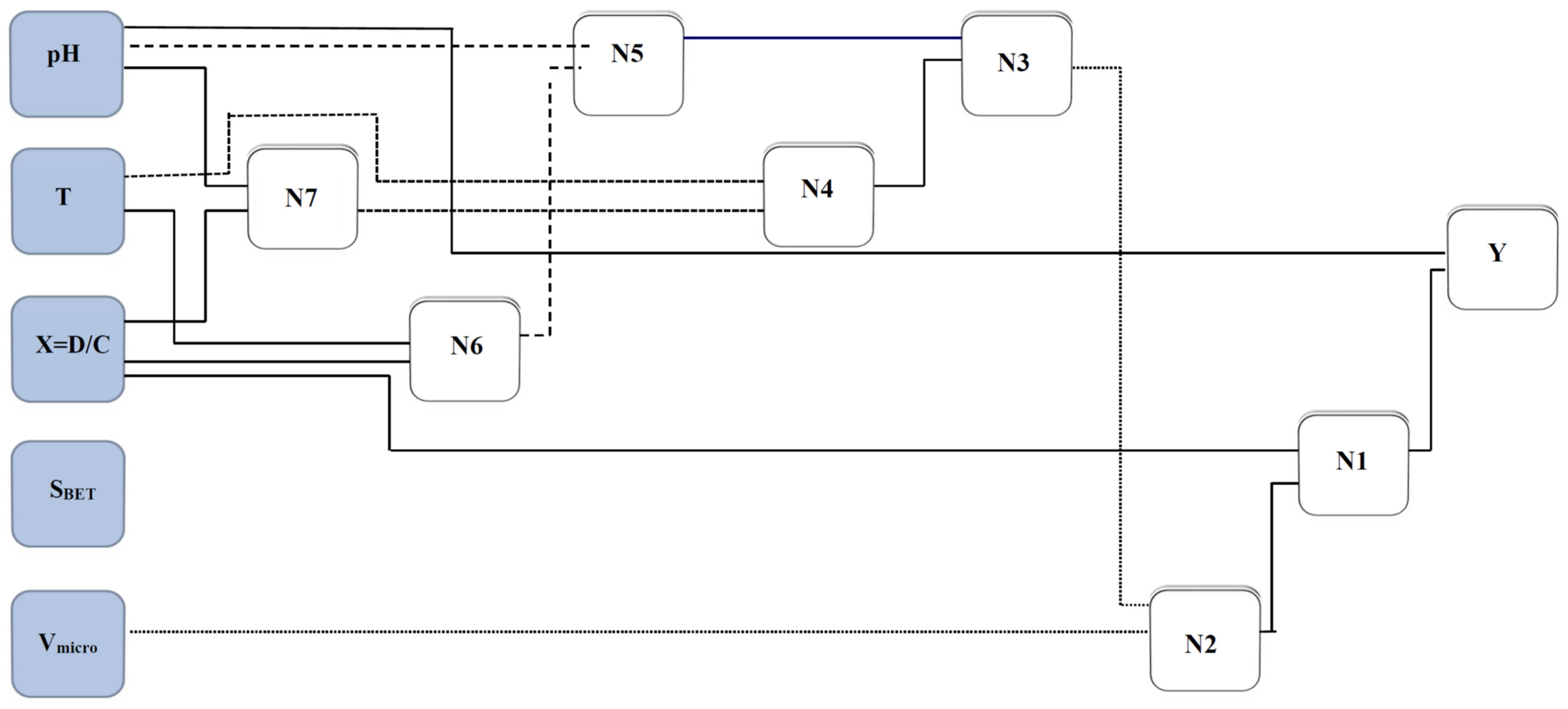
2.2.3. Group Method of Data Handling (GMDH)
2.3. Optimization Approaches
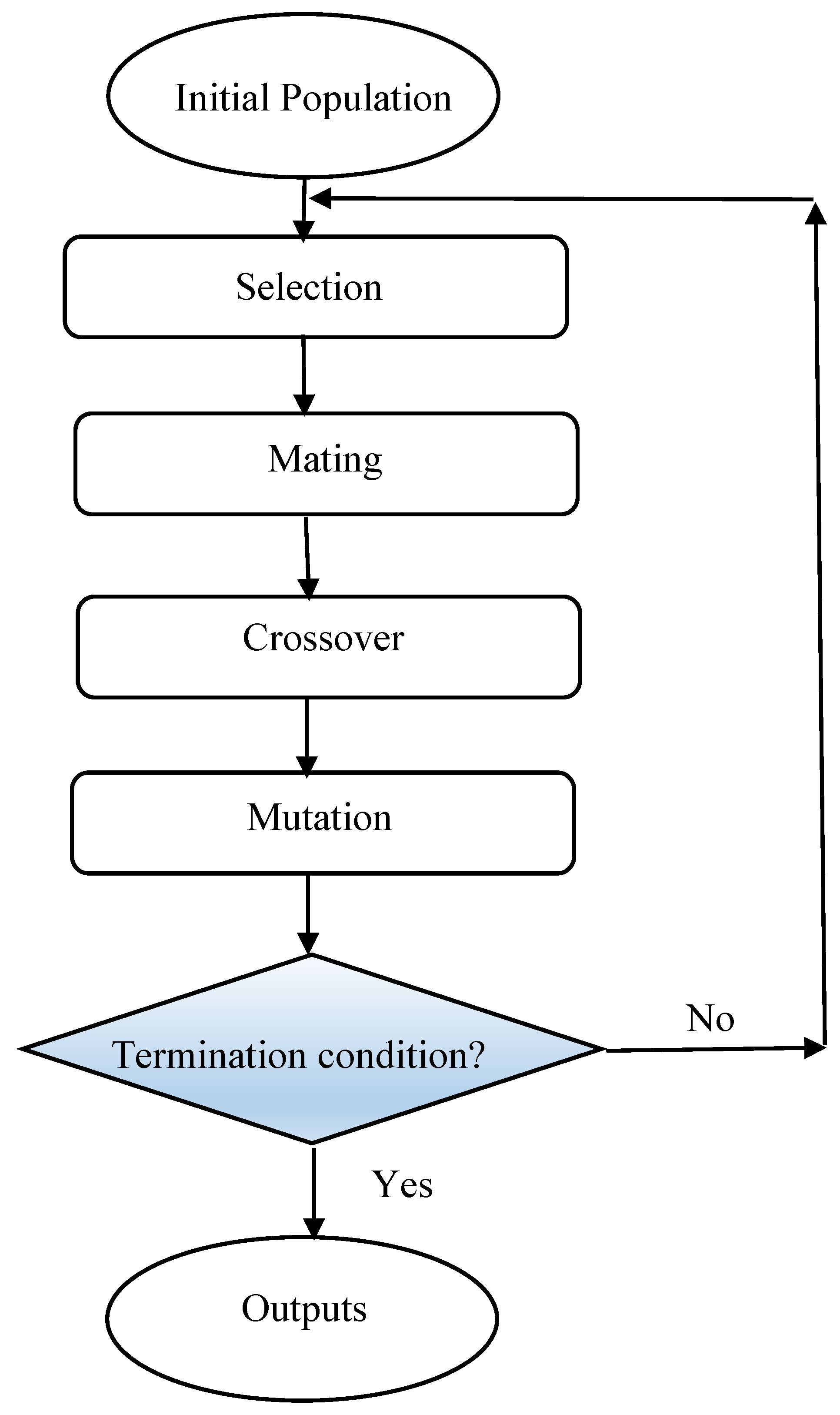
2.3.1. Genetic Algorithm
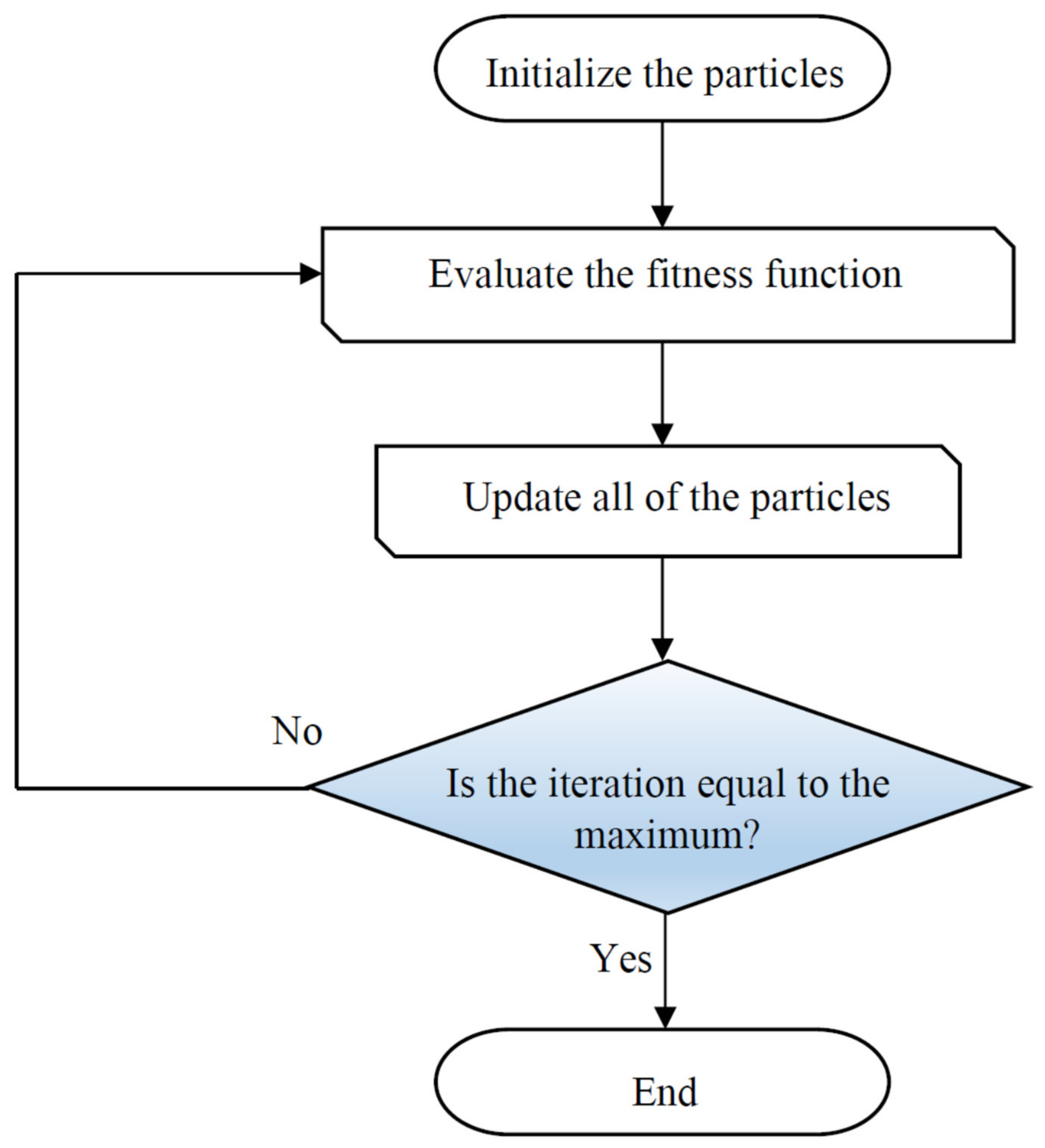
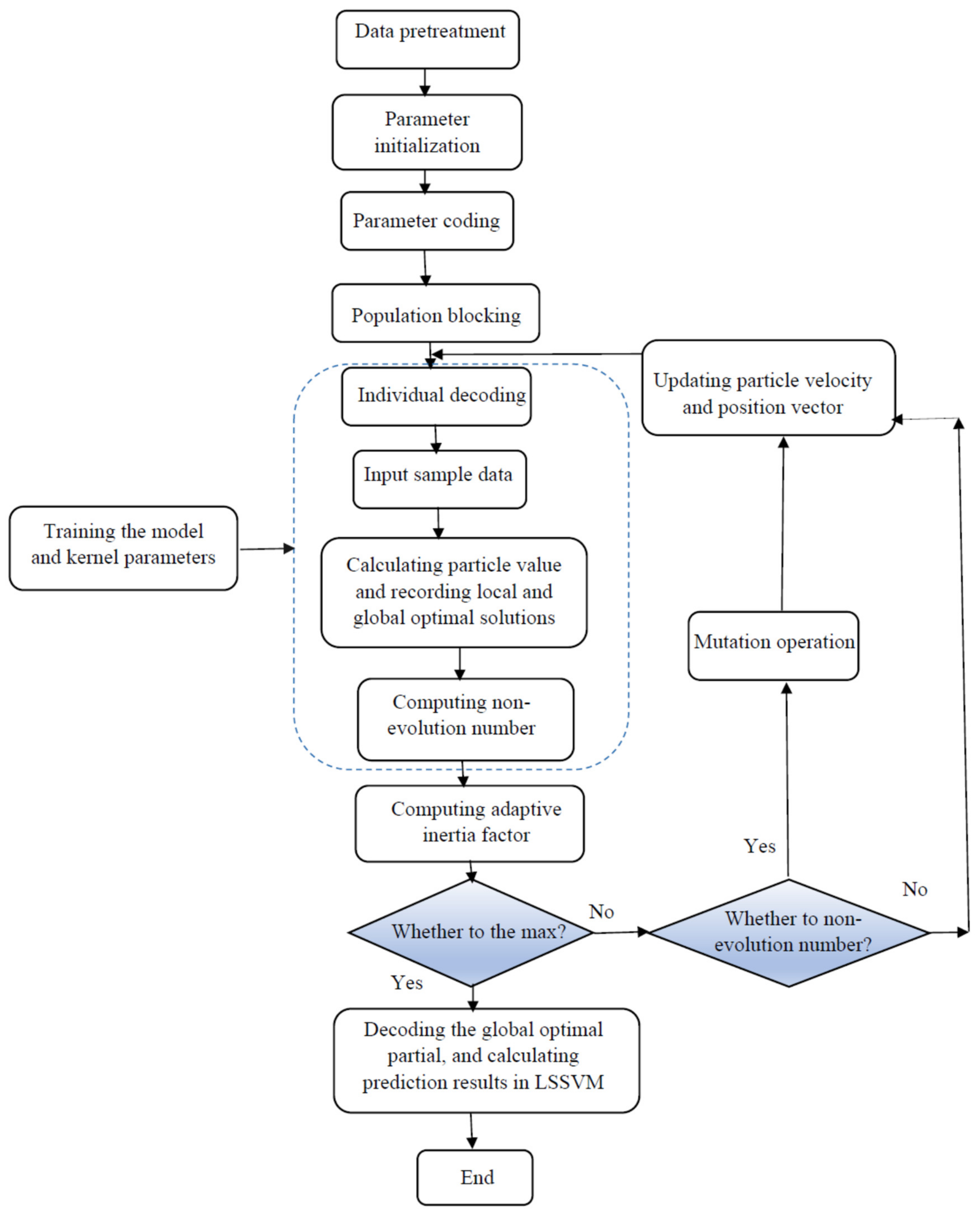
2.3.2. Particle Swarm Optimization
2.3.3. Coupled Simulated Annealing
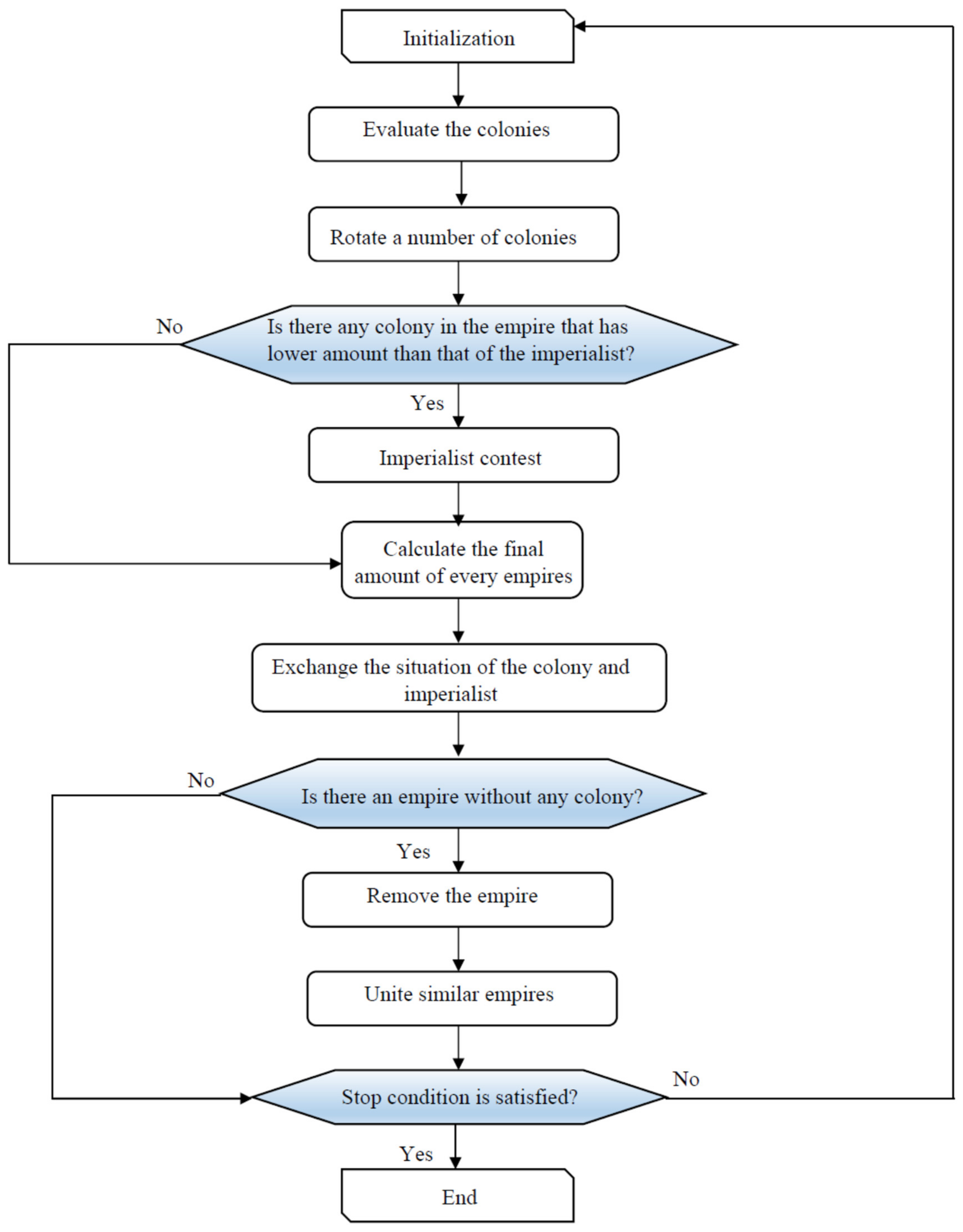
2.3.4. Imperialistic Competitive Algorithm
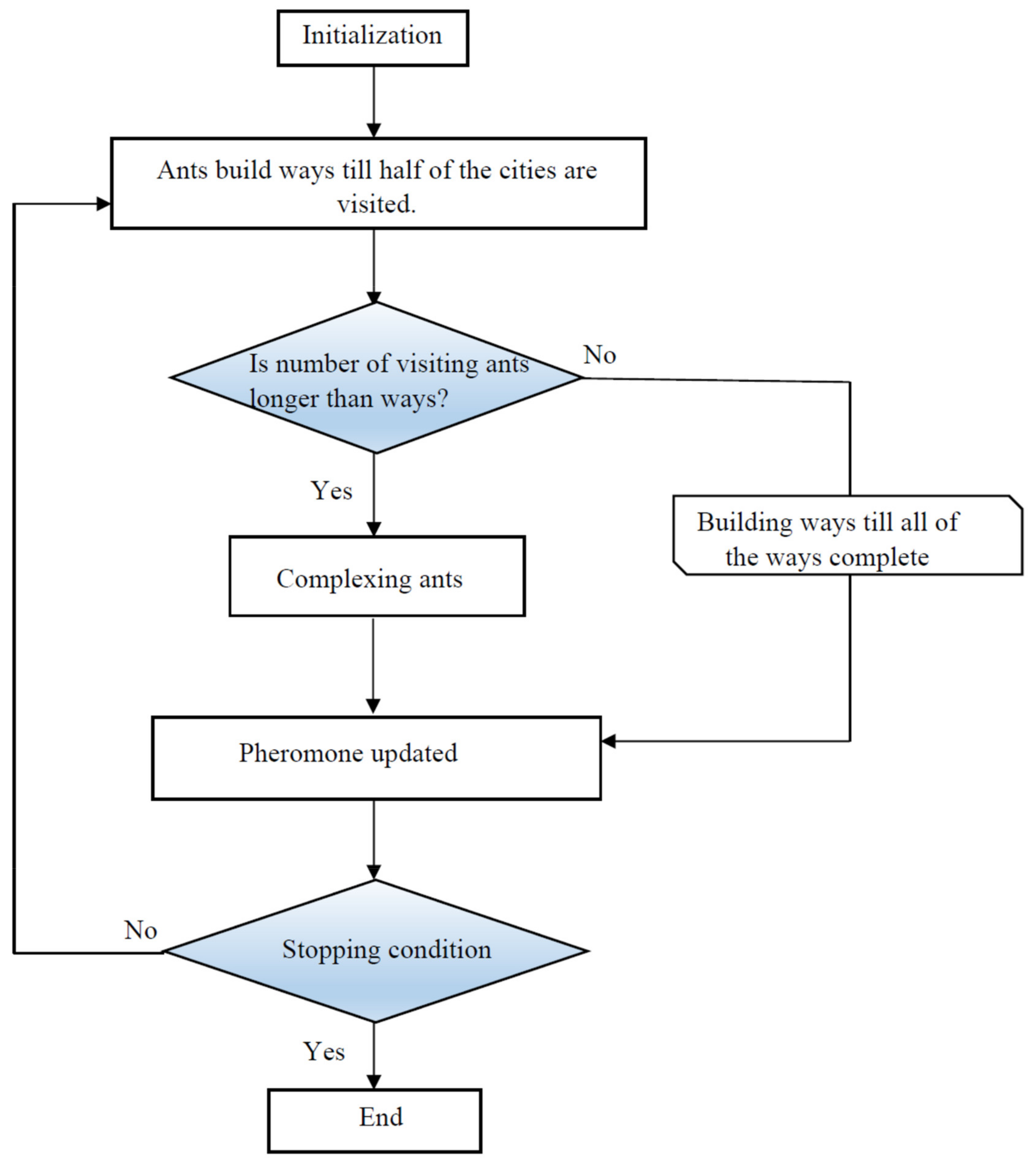
2.3.5. Ant Colony Optimization
- For N number of selected random solutions, the OF should be determined.
- The best and worst initial solutions are denoted by x1 and xN, respectively, which are necessary to organize the solution.
- The following expression is used to assign a weight for each individual solution:
- 4.
- Then, the Gaussian composite probabilistic modeling is constructed based on the following expression:
- 5.
- The M samples as the solution offspring are created by the multidimensional model, as given below:
- 6.
- The M offspring and n best solution are chosen.
- 7.
- The termination criterion is checked.
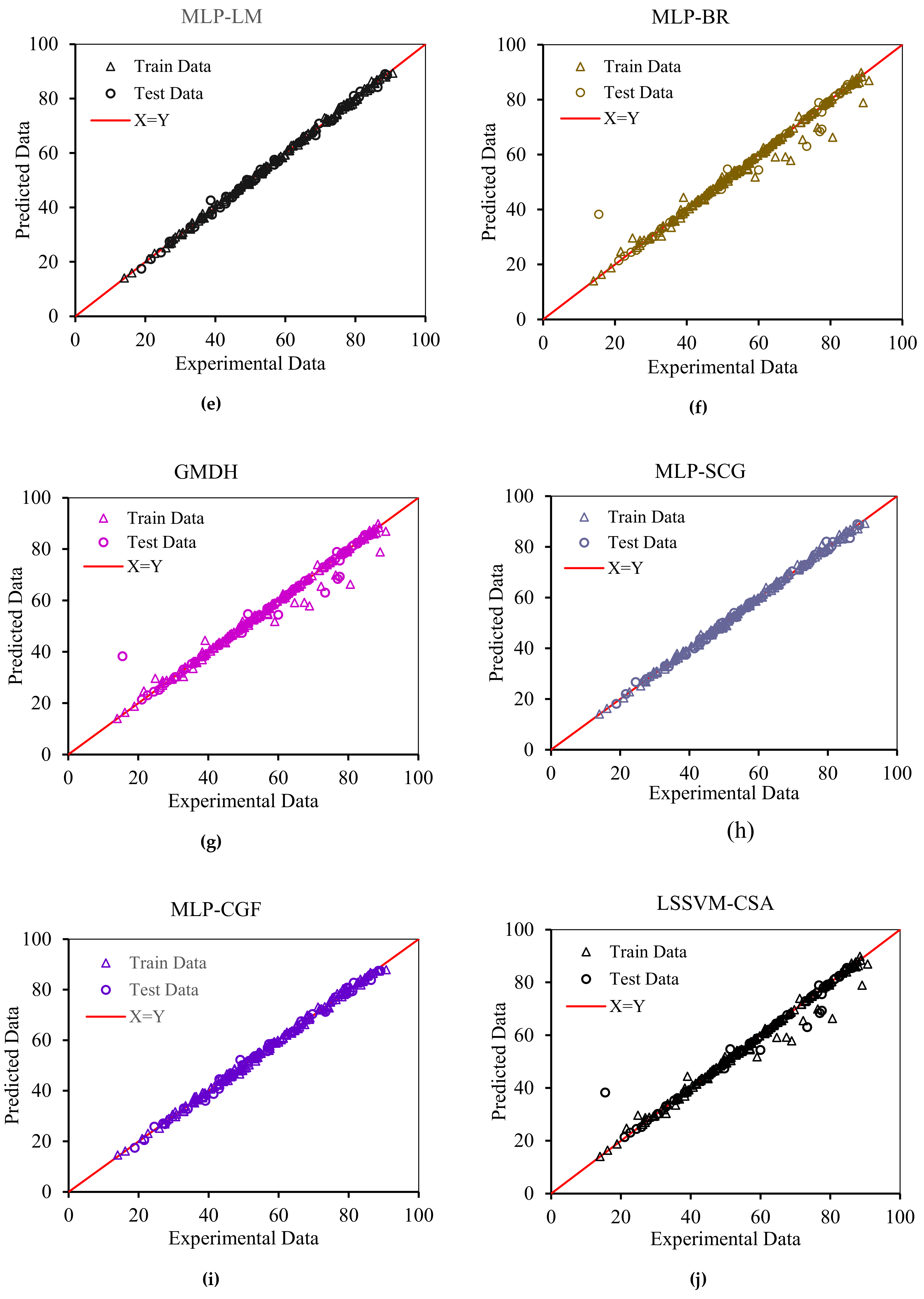
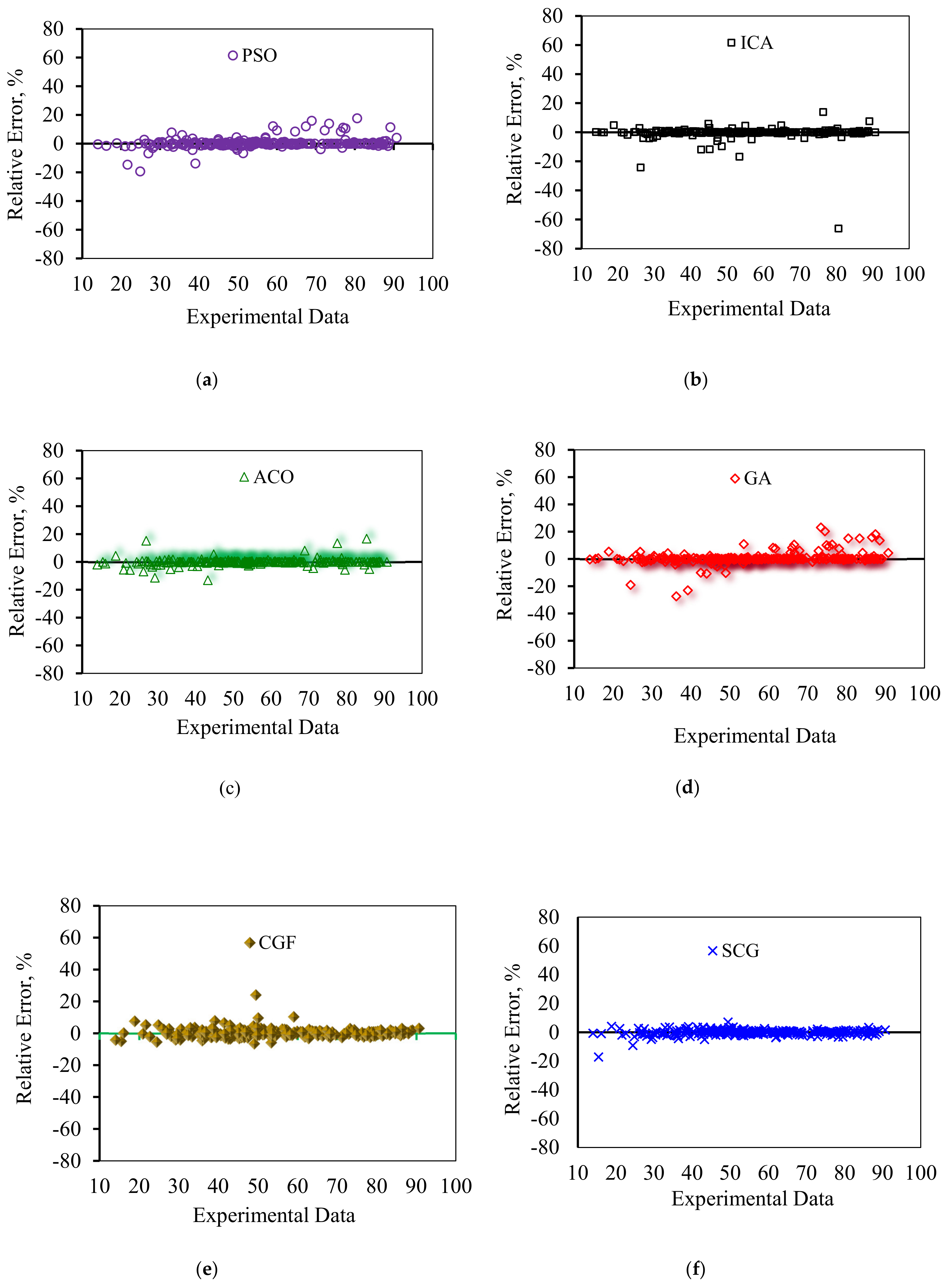
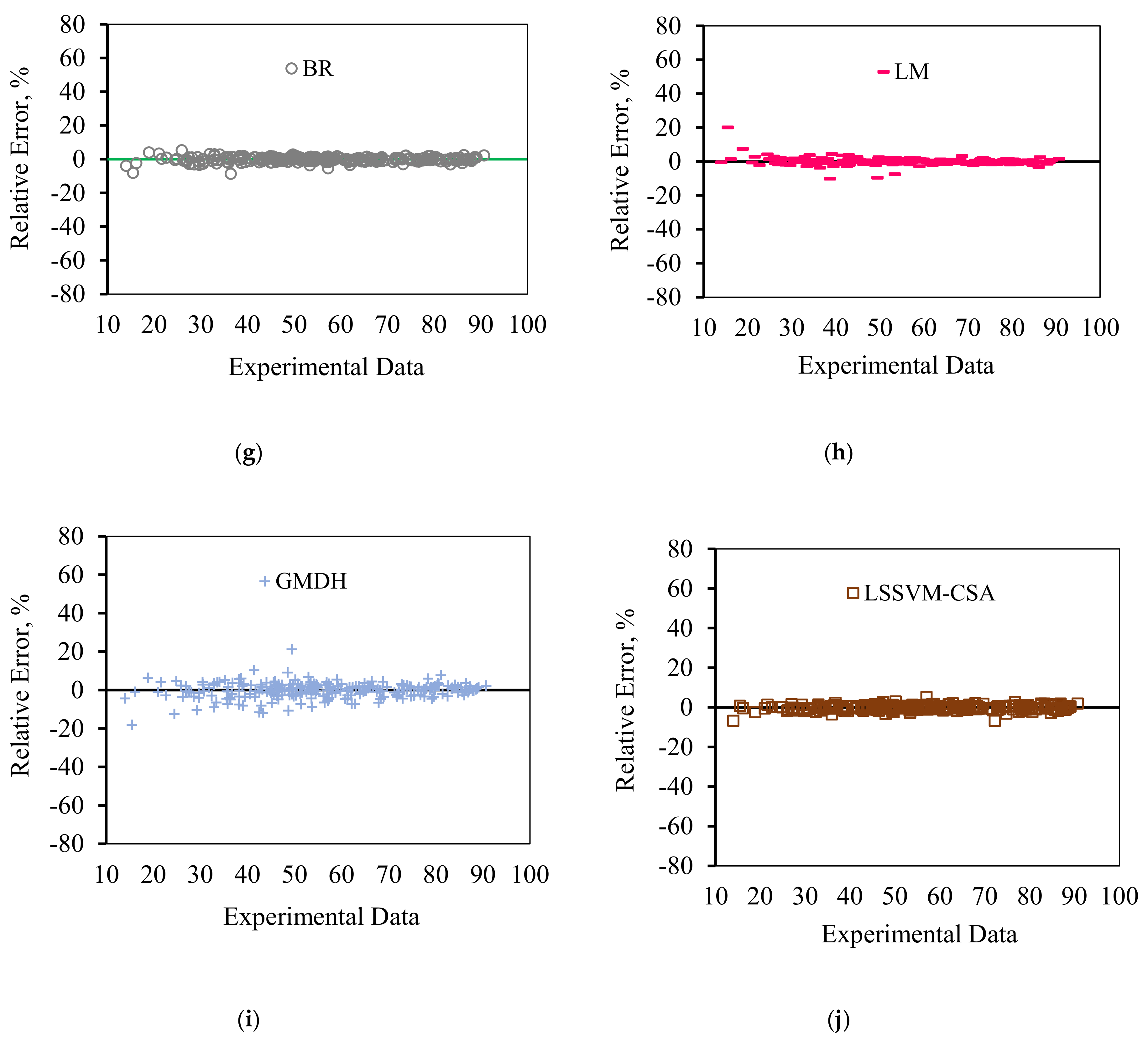
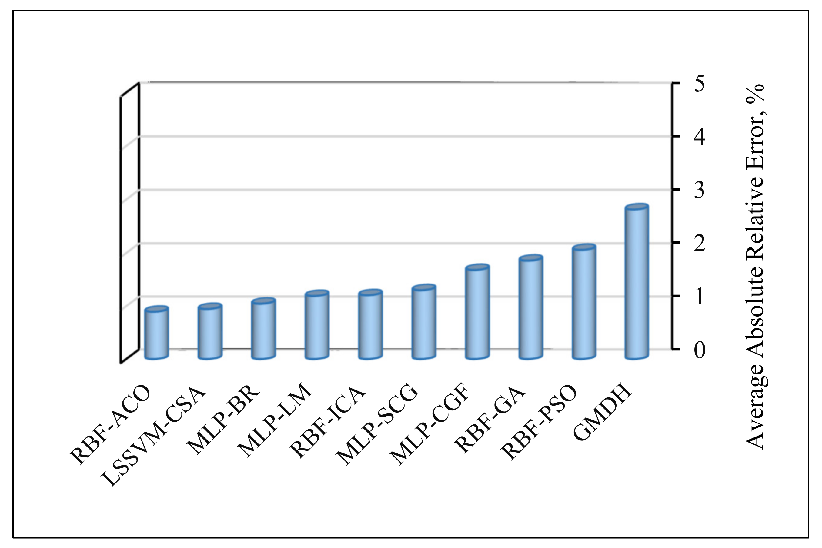
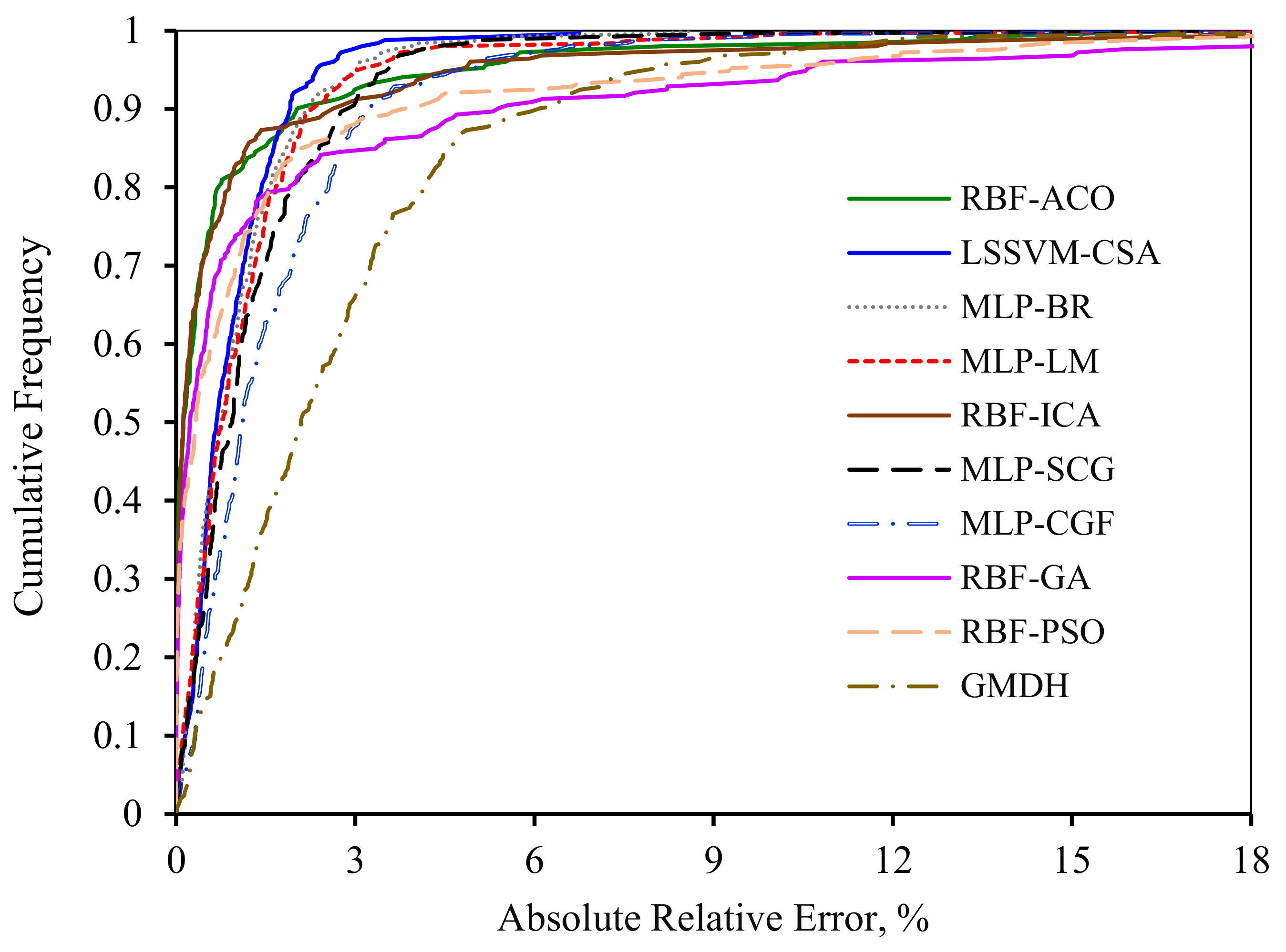
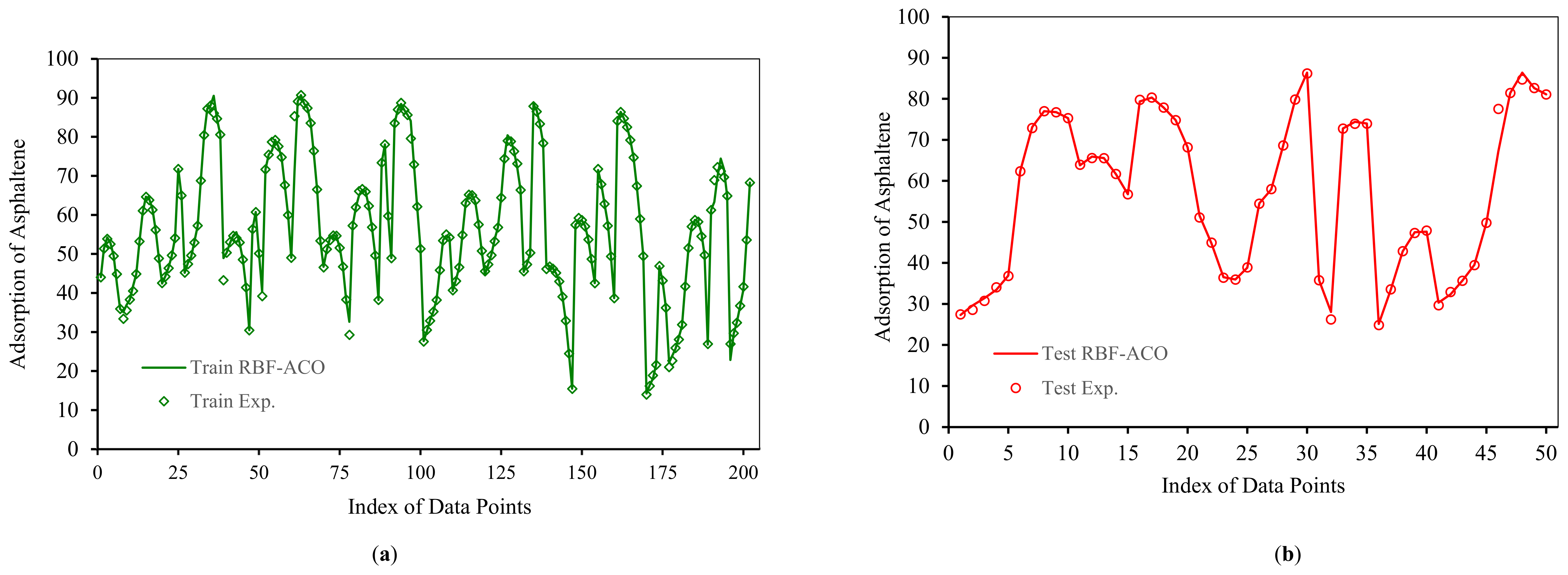
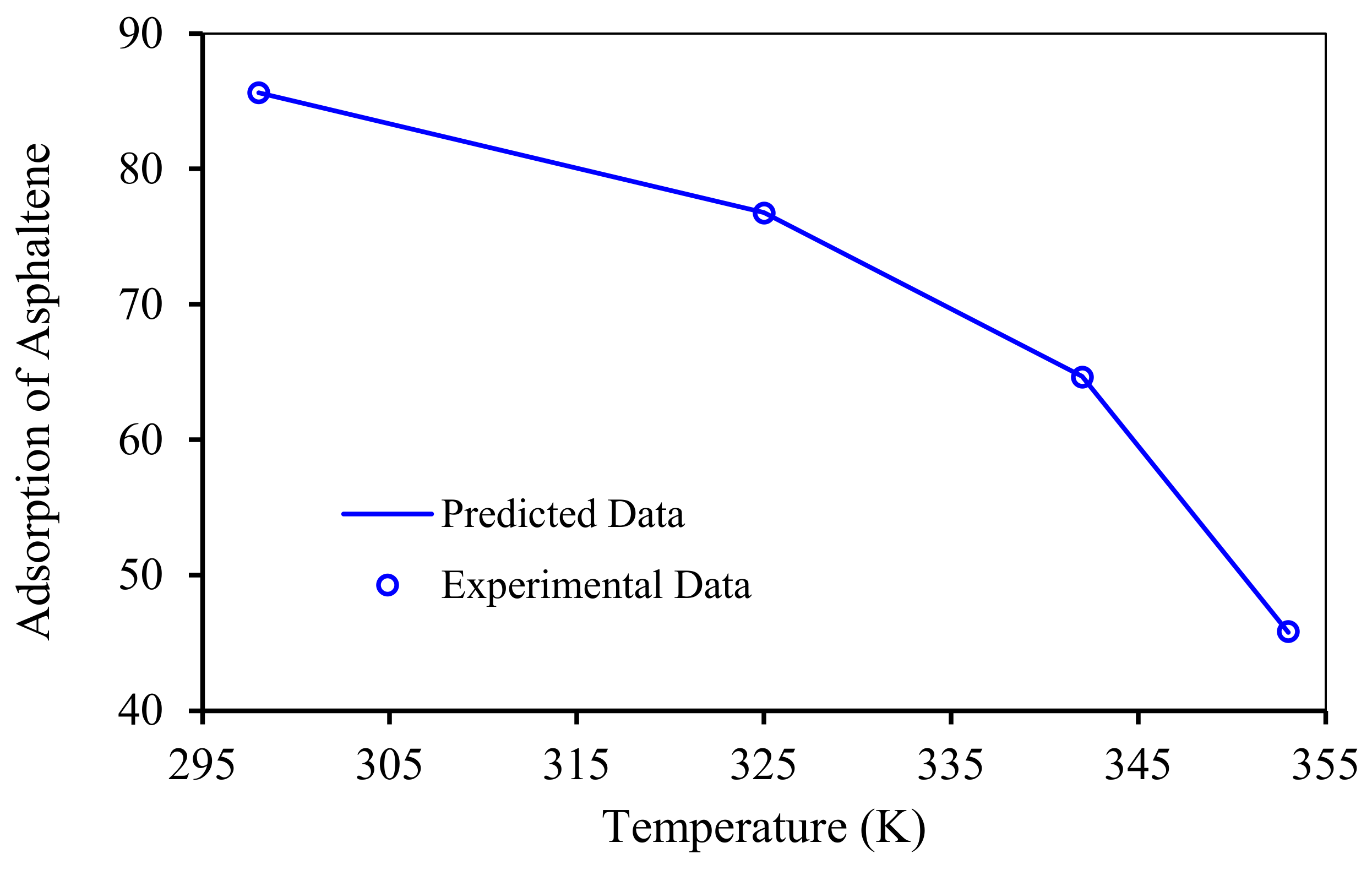
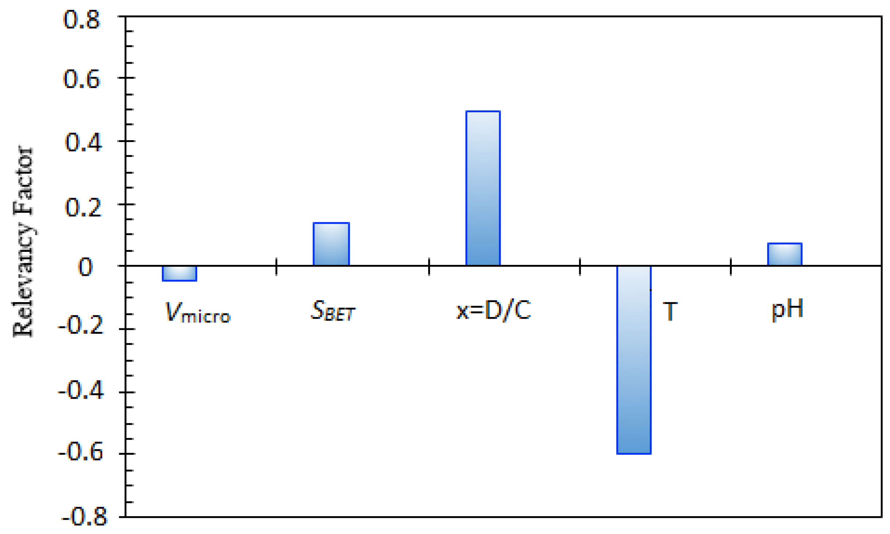
3. Results and Discussion
4. Conclusions
Author Contributions
Funding
Conflicts of Interest
Nomenclatures
| A a × b | matrix in Hat matrix |
| a | Number of algorithm samples |
| AAPRE | Average absolute percent relative error |
| ACO | Ant colony optimization |
| ANN | Artificial neural network |
| ANFIS | Adaptive neuro-fuzzy inference system |
| APRE | Average percent relative error |
| b | Number of algorithm parameters |
| BR | Bayesian regularization |
| c1 | Relative impact of the social components |
| c2 | Relative impact of the cognitive components |
| CGF | Conjugate gradient with Fletcher- Reeves updates |
| CSA | Coupled simulated annealing |
| Combinatorial vector | |
| gbest | Best global position |
| GA | Genetic algorithm |
| GMDH | Group method of data handling |
| H | Hat matrix |
| Leverage limit | |
| ICA | Imperialistic competitive algorithm |
| ISC | In situ combustion |
| LIBS | Laser-Induced Breakdown Spectroscopy |
| LM | Levenberg-Marquardt |
| LSSVM | Least-squares support vector machine |
| MLP | Multilayer perceptron |
| MW | Molecular weight |
| Nimp | Imperialists size |
| NPs | Nanoparticles |
| NTC | Normalized TC |
| OF | Objective function |
| pbest | Best visited position |
| PNN | Polynomial neural network |
| PPn | Imperialists possession probability |
| PSO | Particle swarm optimization |
| A random number vector | |
| Relevancy factor | |
| R2 | Coefficient of determination |
| RBF | Radial basis function |
| RMSE | Root-mean-square error |
| SBET | BET surface area |
| SA | Simulated annealing |
| SCG | Scaled conjugate gradient |
| SD | Standard deviation |
| TC | Total cost value |
| Velocity of a particle | |
| i-th input value of the k-th input parameter | |
| Average value for the k-th input | |
| i-th output value | |
| Average value for output parameter |
Greek Letters
| Regularization parameter | |
| Weight matrix | |
| Slack variable | |
| Kernel function | |
| Radial basis function | |
| αK | Lagrangian multipliers |
| σ | Gaussian spread |
References
- Hajizadeh, A.; Ravari, R.R.; Amani, M.; Shedid, S.A. An Investigation on Asphaltene Precipitation Potential for Light and Heavy Oils, During Natural Depletion. In Proceedings of the Nigeria Annual International Conference and Exhibition, Rome, Italy, 9–12 June 2008; Society of Petroleum Engineers: Dallas, TX, USA, 2008. [Google Scholar] [CrossRef] [Green Version]
- Bouhadda, Y.; Bormann, D.; Sheu, E.; Bendedouch, D.; Krallafa, A.; Daaou, M. Characterization of Algerian Hassi-Messaoud asphaltene structure using Raman spectrometry and X-ray diffraction. Fuel 2007, 86, 1855–1864. [Google Scholar] [CrossRef]
- Speight, J. Petroleum Asphaltenes-Part 1: Asphaltenes, resins and the structure of petroleum. Oil Gas Sci. Technol. 2004, 59, 467–477. [Google Scholar] [CrossRef] [Green Version]
- Young, D.W.; Stacey, M.J. Petroleum fuel additives: A case for recognition. Appl. Energy 1978, 4, 51–73. [Google Scholar] [CrossRef]
- Gondal, M.A.; Siddiqui, M.N.; Nasr, M.M. Detection of trace metals in asphaltenes using an advanced laser-induced breakdown spectroscopy (LIBS) technique. Energy Fuels 2010, 24, 1099–1105. [Google Scholar] [CrossRef]
- Alboudwarej, H.; Beck, J.; Svrcek, W.Y.; Yarranton, H.W.; Akbarzadeh, K. Sensitivity of asphaltene properties to separation techniques. Energy Fuels 2002, 16, 462–469. [Google Scholar] [CrossRef]
- Speight, J.G. Asphaltenes and the structure of petroleum. In Petroleum Chemistry and Refining; Taylor & Francis: Abingdon, UK, 1998; pp. 103–120. [Google Scholar]
- Marczewski, A.W.; Szymula, M. Adsorption of asphaltenes from toluene on mineral surface. Colloids Surf. A: Physicochem. Eng. Asp. 2002, 208, 259–266. [Google Scholar] [CrossRef] [Green Version]
- Groenzin, H.; Mullins, O.C. Asphaltene molecular size and structure. J. Phys. Chem. A 1999, 103, 11237–11245. [Google Scholar] [CrossRef]
- McKenna, A.M.; McKenna, A.M.; Blakney, G.T.; Xian, F.; Glaser, P.B.; Rodgers, R.P.; Marshall, A.G. Heavy petroleum composition. 2. Progression of the Boduszynski model to the limit of distillation by ultrahigh-resolution FT-ICR mass spectrometry. Energy Fuels 2010, 24, 2939–2946. [Google Scholar] [CrossRef]
- Mullins, O.C.; Sabbah, H.; Eyssautier, J.; Pomerantz, A.E.; Barré, L.; Andrews, A.B.; Ruiz-Morales, Y.; Mostowfi, F.; McFarlane, R.; Goual, L.; et al. Advances in asphaltene science and the Yen–Mullins model. Energy Fuels 2012, 26, 3986–4003. [Google Scholar] [CrossRef]
- Guzman, A.; Bueno, A.; Carbognani, L. Molecular weight determination of asphaltenes from Colombian crudes by size exclusion chromatography (SEC) and vapor pressure osmometry (VPO). Pet. Sci. Technol. 2009, 27, 801–816. [Google Scholar] [CrossRef]
- Yarranton, H.W.; Alboudwarej, H.; Jakher, R. Investigation of asphaltene association with vapor pressure osmometry and interfacial tension measurements. Ind. Eng. Chem. Res. 2000, 39, 2916–2924. [Google Scholar] [CrossRef]
- Qian, K.; Edwards, K.E.; Siskin, M.; Olmstead, W.N.; Mennito, A.S.; Dechert, G.J.; Hoosain, N.E. Desorption and ionization of heavy petroleum molecules and measurement of molecular weight distributions. Energy Fuels 2007, 21, 1042–1047. [Google Scholar] [CrossRef]
- Andersen, S.I. 18 Association of Petroleum Asphaltenes and the Effect on Solution Properties. In Surface and Colloid Chemistry; CRC Press: Boca Raton, FL, USA, 2009; p. 703. [Google Scholar]
- da Costa, L.M.; Stoyanov, S.R.; Gusarov, S.; Tan, X.; Gray, M.R.; Stryker, J.M.; Tykwinski, R.; de M. Carneiro, J.W.; Seidl, P.R.; Kovalenko, A. Density functional theory investigation of the contributions of π–π stacking and hydrogen-bonding interactions to the aggregation of model asphaltene compounds. Energy Fuels 2012, 26, 2727–2735. [Google Scholar] [CrossRef]
- Zahabi, A.; Gray, M.R.; Czarnecki, J.; Dabros, T. Flocculation of silica particles from a model oil solution: Effect of adsorbed asphaltenes. Energy Fuels 2010, 24, 3616–3623. [Google Scholar] [CrossRef]
- Turgman-Cohen, S.; Smith, M.B.; Fischer, D.A.; Kilpatrick, P.K.; Genzer, J. Asphaltene adsorption onto self-assembled monolayers of mixed aromatic and aliphatic trichlorosilanes. Langmuir 2009, 25, 6260–6269. [Google Scholar] [CrossRef] [PubMed]
- Jouault, N.; Corvis, Y.; Cousin, F.; Jestin, J.; Barré, L. Asphaltene adsorption mechanisms on the local scale probed by neutron reflectivity: Transition from monolayer to multilayer growth above the flocculation threshold. Langmuir 2009, 25, 3991–3998. [Google Scholar] [CrossRef] [PubMed]
- Adams, J.J. Asphaltene adsorption, a literature review. Energy Fuels 2014, 28, 2831–2856. [Google Scholar] [CrossRef]
- Briones, A.M. Asphaltene Adsorption on Different Solid Surfaces from Organic Solvents. Master’s Thesis, University of Alberta, Edmonton, Canada, 2016. [Google Scholar] [CrossRef]
- Akbarzadeh, K.; Hammami, A.; Kharrat, A.; Zhang, D.; Allenson, S.; Creek, J.; Kabir, S.; Jamaluddin, A.; Marshall, A.G.; Rodgers, R.P.; et al. Asphaltenes—Problematic but rich in potential. Oilfield Rev. 2007, 19, 22–43. [Google Scholar]
- Syunyaev, R.; Balabin, R.M.; Akhatov, I.S.; Safieva, J.O. Adsorption of petroleum asphaltenes onto reservoir rock sands studied by near-infrared (NIR) spectroscopy. Energy Fuels 2009, 23, 1230–1236. [Google Scholar] [CrossRef]
- Leontaritis, K.J.; Mansoori, G.A. Asphaltene flocculation during oil production and processing: A thermodynamic collodial model. In Proceedings of the SPE International Symposium on Oilfield Chemistry, San Antonio, TX, USA, 4–6 February 1987; Society of Petroleum Engineers: Dallas, TX, USA, 1987. [Google Scholar] [CrossRef]
- Saraji, S.; Goual, L.; Piri, M. Adsorption of asphaltenes in porous media under flow conditions. Energy Fuels 2010, 24, 6009–6017. [Google Scholar] [CrossRef]
- Gawel, I.; Bociarska, D.; Biskupski, P. Effect of asphaltenes on hydroprocessing of heavy oils and residua. Appl. Catal. A: Gen. 2005, 295, 89–94. [Google Scholar] [CrossRef]
- Moreira, L.F.B.; Lucas, E.F.; González, G. Stabilization of asphaltenes by phenolic compounds extracted from cashew-nut shell liquid. J. Appl. Polym. Sci. 1999, 73, 29–34. [Google Scholar] [CrossRef]
- da Silva Ramos, A.C.; Haraguchi, L.; Notrispe, F.R.; Loh, W.; Mohamed, R.S. Interfacial and colloidal behavior of asphaltenes obtained from Brazilian crude oils. J. Pet. Sci. Eng. 2001, 32, 201–216. [Google Scholar] [CrossRef]
- Junior, L.C.R.; Ferreira, M.S.; Ramos, A.C.d. Inhibition of asphaltene precipitation in Brazilian crude oils using new oil soluble amphiphiles. J. Pet. Sci. Eng. 2006, 51, 26–36. [Google Scholar] [CrossRef]
- Kelland, M.A. Production Chemicals for the Oil and Gas Industry; CRC Press: Boca Raton, FL, USA, 2014. [Google Scholar]
- Balson, T.; Craddock, H.A.; Dunlop, J.; Frampton, H.; Payne, G.; Reid, P.; Asomaning, S.; Yen, A. Prediction and solution of asphaltene related problems in the field. In Chemistry in the Oil Industry VII; Royal Society of Chemistry: Cambridge, UK, 2002; pp. 277–286. [Google Scholar] [CrossRef]
- Almehaideb, R.A.; Zekri, A.Y. Possible use of bacteria/steam to treat asphaltene deposition in carbonate rocks. In Proceedings of the SPE European Formation Damage Conference, Hague, The Netherlands, 21–22 May 2001; Society of Petroleum Engineers: Dallas, TX, USA, 2001. [Google Scholar] [CrossRef]
- Akbar, S.; Saleh, A. A comprehensive approach to solve asphaltene deposition problem in some deep wells. In Middle East Oil Show; Society of Petroleum Engineers: Dallas, TX, USA, 1989. [Google Scholar] [CrossRef]
- Zekri, A.Y.; Shedid., S.A.; Alkashef, H. Use of laser technology for the treatment of asphaltene deposition in carbonate formations. Pet. Sci. Technol. 2003, 21, 1409–1426. [Google Scholar] [CrossRef]
- Voloshin, A.I.; Ragulin, V.V.; Telin, A.G. Development and Introduction of Heavy Organic Compound Deposition Diagnostics, Prevention and Removing. In SPE International Symposium on Oilfield Chemistry; Society of Petroleum Engineers: Dallas, TX, USA, 2005. [Google Scholar] [CrossRef]
- Salehzadeh, M.; Akherati, A.; Ameli, F.; Dabir, B. Experimental study of ultrasonic radiation on growth kinetic of asphaltene aggregation and deposition. Can. J. Chem. Eng. 2016, 94, 2202–2209. [Google Scholar] [CrossRef]
- Shedid, S.A. An ultrasonic irradiation technique for treatment of asphaltene deposition. J. Pet. Sci. Eng. 2004, 42, 57–70. [Google Scholar] [CrossRef]
- Miadonye, A.; Evans, L. The solubility of asphaltenes in different hydrocarbon liquids. Pet. Sci. Technol. 2010, 28, 1407–1414. [Google Scholar] [CrossRef]
- Bernadiner, M. Advanced asphaltene and paraffin control technology. In SPE International Symposium on Oilfield Chemistry; Society of Petroleum Engineers: Dallas, TX, USA, 1993. [Google Scholar] [CrossRef]
- Abedini, A.; Ashoori, S.; Torabi, F.; Saki, Y.; Dinarvand, N. Mechanism of the reversibility of asphaltene precipitation in crude oil. J. Pet. Sci. Eng. 2011, 78, 316–320. [Google Scholar] [CrossRef]
- Nassar, N.N.; Husein, M.M.; Pereira-Almao, P. In-situ prepared nanoparticles in support of oilsands industry meeting future environmental challenges. Explor. Prod. Oil Gas Rev. 2011, 9, 46–48. [Google Scholar]
- Etim, U.J.; Bai, P.; Yan, Z. Nanotechnology applications in petroleum refining. In Nanotechnology in Oil and Gas Industries; Springer: Berlin/Heidelberg, Germany, 2018; pp. 37–65. [Google Scholar] [CrossRef]
- Ezeonyeka, N.L.; Hemmati-Sarapardeh, A.; Husein, M.M. Asphaltenes adsorption onto metal oxide nanoparticles: A critical evaluation of measurement techniques. Energy Fuels 2018, 32, 2213–2223. [Google Scholar] [CrossRef]
- Nassar, N.N.; Hassan, A.; Pereira-Almao, P. Clarifying the catalytic role of NiO nanoparticles in the oxidation of asphaltenes. Appl. Catal. A: Gen. 2013, 462, 116–120. [Google Scholar] [CrossRef]
- Nassar, N.N.; Hassan, A.; Carbognani, L.; Lopez-Linares, F.; Pereira-Almao, P. Iron oxide nanoparticles for rapid adsorption and enhanced catalytic oxidation of thermally cracked asphaltenes. Fuel 2012, 95, 257–262. [Google Scholar] [CrossRef]
- Rezaei, M.; Schaffie, M.; Ranjbar, M. Thermocatalytic in situ combustion: Influence of nanoparticles on crude oil pyrolysis and oxidation. Fuel 2013, 113, 516–521. [Google Scholar] [CrossRef]
- Nassar, N.N.; Franco, C.A.; Montoya, T.; Cortés, F.B.; Hassan, A. Effect of oxide support on Ni–Pd bimetallic nanocatalysts for steam gasification of n-C7 asphaltenes. Fuel 2015, 156, 110–120. [Google Scholar] [CrossRef]
- Nassar, N.N.; Hassan, A.; Pereira-Almao, P. Application of nanotechnology for heavy oil upgrading: Catalytic steam gasification/cracking of asphaltenes. Energy Fuels 2011, 25, 1566–1570. [Google Scholar] [CrossRef]
- Abdeen, D.H.; El Hachach, M.; Koc, M.; Atieh, M.A. A Review on the Corrosion Behaviour of Nanocoatings on Metallic Substrates. Materials 2019, 12, 210. [Google Scholar] [CrossRef] [Green Version]
- Kadhim, M.; Sukkar, K.A.; Abbas, A.S.; Obaeed, N.H. Investigation Nano coating for Corrosion Protection of Petroleum Pipeline Steel Type A106 Grade B; Theoretical and Practical Study in Iraqi Petroleum Sector. Eng. Technol. J. 2017, 35, 1042–1051. [Google Scholar]
- Romero, Z.; Disney, R.; Acuna, H.M.; Cortes, F.; Patino, J.E.; Cespedes Chavarro, C.; Mora, E.; Botero, O.F.; Guarin, L. Application and evaluation of a nanofluid containing nanoparticles for asphaltenes inhibition in well CPSXL4. In Proceedings of the OTC Brasil, Offshore Technology Conference, Rio de Janeiro, Brazil, 29–31 October 2013. [Google Scholar] [CrossRef]
- Madhi, M.; Bemani, A.; Daryasafar, A.; Khosravi Nikou, M.R. Experimental and modeling studies of the effects of different nanoparticles on asphaltene adsorption. Pet. Sci. Technol. 2017, 35, 242–248. [Google Scholar] [CrossRef]
- Nassar, N.N.; Al-Jabari, M.E.; Husein, M.M. Removal of asphaltenes from heavy oil by nickel nano and micro particle adsorbents. In Proceedings of the IASTED International Conference, Crete, Greece, 29 September–1 October 2008. [Google Scholar]
- Nassar, N.N.; Hassan, A.; Pereira-Almao, P. Comparative oxidation of adsorbed asphaltenes onto transition metal oxide nanoparticles. Colloids Surf. A Physicochem. Eng. Asp. 2011, 384, 145–149. [Google Scholar] [CrossRef]
- Nassar, N.N.; Hassan, A.; Pereira-Almao, P. Metal oxide nanoparticles for asphaltene adsorption and oxidation. Energy Fuels 2011, 25, 1017–1023. [Google Scholar] [CrossRef]
- Abu Tarboush, B.J.; Husein, M.M. Adsorption of asphaltenes from heavy oil onto in situ prepared NiO nanoparticles. J. Colloid Interface Sci. 2012, 378, 64–69. [Google Scholar] [CrossRef]
- Tarboush, B.J.A. and M.M. Husein, Dispersed Fe2O3 nanoparticles preparation in heavy oil and their uptake of asphaltenes. Fuel Process. Technol. 2015, 133, 120–127. [Google Scholar] [CrossRef]
- Hosseinpour, N.; Khodadadi, A.A.; Bahramian, A.; Mortazavi, Y. Asphaltene adsorption onto acidic/basic metal oxide nanoparticles toward in situ upgrading of reservoir oils by nanotechnology. Langmuir 2013, 29, 14135–14146. [Google Scholar] [CrossRef]
- Nassar, N.N.; Hassan, A.; Pereira-Almao, P. Effect of surface acidity and basicity of aluminas on asphaltene adsorption and oxidation. J. Colloid Interface Sci. 2011, 360, 233–238. [Google Scholar] [CrossRef]
- Franco, C.A.; Lozano, M.M.; Acevedo, S.; Nassar, N.N.; Cortés, F.B. Effects of resin I on asphaltene adsorption onto nanoparticles: A novel method for obtaining asphaltenes/resin isotherms. Energy Fuels 2015, 30, 264–272. [Google Scholar] [CrossRef]
- Sedighi, M.; Mohammadi, M.; Sedighi, M. Green SAPO-5 supported NiO nanoparticles as a novel adsorbent for removal of petroleum asphaltenes: Financial assessment. J. Pet. Sci. Eng. 2018, 171, 1433–1442. [Google Scholar] [CrossRef]
- Sedighi, M.; Mohammadi, M.; Sedighi, M.; Ghasemi, M. Biobased cadaverine as a green template in the synthesis of NiO/ZSM-5 nanocomposites for removal of petroleum asphaltenes: Financial analysis, isotherms, and kinetics study. Energy Fuels 2018, 32, 7412–7422. [Google Scholar] [CrossRef]
- Mohammadi, M.; Safari, M.; Ghasemi, M.; Daryasafar, A.; Sedighi, M. Asphaltene adsorption using green nanocomposites: Experimental study and adaptive neuro-fuzzy interference system modeling. J. Pet. Sci. Eng. 2019, 177, 1103–1113. [Google Scholar] [CrossRef]
- Mohammadi, M.; Sedighi, M.; Hemati, M. Removal of petroleum asphaltenes by improved activity of NiO nanoparticles supported on green AlPO-5 zeolite: Process optimization and adsorption isotherm. Petroleum 2019. [Google Scholar] [CrossRef]
- Suykens, J.A.; Vandewalle, J. Least squares support vector machine classifiers. Neural Process. Lett. 1999, 9, 293–300. [Google Scholar] [CrossRef]
- Eslamimanesh, A.; Gharagheizi, F.; Illbeigi, M.; Mohammadi, A.H.; Fazlali, A.; Richon, D. Phase equilibrium modeling of clathrate hydrates of methane, carbon dioxide, nitrogen, and hydrogen+ water soluble organic promoters using Support Vector Machine algorithm. Fluid Phase Equilibria 2012, 316, 34–45. [Google Scholar] [CrossRef]
- Eslamimanesh, A.; Gharagheizi, F.; Mohammadi, A.H.; Richon, D. Phase equilibrium modeling of structure H clathrate hydrates of methane+ water “insoluble” hydrocarbon promoter using QSPR molecular approach. J. Chem. Eng. Data 2011, 56, 3775–3793. [Google Scholar] [CrossRef]
- Bemani, A.; Baghban, A.; Mohammadi, A.H. An insight into the modeling of sulfur content of sour gases in supercritical region. J. Pet. Sci. Eng. 2020, 184, 106459. [Google Scholar] [CrossRef]
- Tatar, A.; Shokrollahi, A.; Mesbah, M.; Rashid, S.; Arabloo, M.; Bahadori, A. Implementing radial basis function networks for modeling CO2-reservoir oil minimum miscibility pressure. J. Nat. Gas Sci. Eng. 2013, 15, 82–92. [Google Scholar] [CrossRef]
- Broomhead, D.S.; Lowe, D. Radial Basis Functions, Multi-Variable Functional Interpolation and Adaptive Networks; Royal Signals and Radar Establishment Malvern: Worcestershire, UK, 1988. [Google Scholar]
- Abdi-Khanghah, M.; Bemani, A.; Naserzadeh, Z.; Zhang, Z. Prediction of solubility of N-alkanes in supercritical CO2 using RBF-ANN and MLP-ANN. J. Co2 Util. 2018, 25, 108–119. [Google Scholar] [CrossRef]
- Shankar, R. The Group Method of Data Handling. Master’s Thesis, University of Delaware, College Park, MD, USA, 1972. [Google Scholar]
- Sawaragi, Y.; Soeda, T.; Tamura, H.; Yoshimura, T.; Ohe, S.; Chujo, Y.; Ishihara, H. Statistical prediction of air pollution levels using non-physical models. Automatica 1979, 15, 441–451. [Google Scholar] [CrossRef]
- Ivakhnenko, A.G. Polynomial theory of complex systems. Ieee Trans. Syst. Man Cybern. 1971, 364–378. [Google Scholar] [CrossRef] [Green Version]
- Atashrouz, S.; Amini, E.; Pazuki, G. Modeling of surface tension for ionic liquids using group method of data handling. Ionics 2015, 21, 1595–1603. [Google Scholar] [CrossRef]
- Atashrouz, S.; Mozaffarian, M.; Pazuki, G. Modeling the thermal conductivity of ionic liquids and ionanofluids based on a group method of data handling and modified Maxwell model. Ind. Eng. Chem. Res. 2015, 54, 8600–8610. [Google Scholar] [CrossRef]
- Madala, H.R. Inductive Learning Algorithms for Complex Systems Modeling: 0; CRC Press: Boca Raton, FL, USA, 2018. [Google Scholar]
- Ivakhnenko, A.; Yurachkovsky, J. Modeling of Complex Systems by Experimental Data. Radio i Svyaz Publishing House, Moscow, 120 Ивахненкo АГ, Юрачкoвский ЮП Мoделирoвание слoжных систем пo экспериментальным данным. М. Радиo и связь 1987, 120. [Google Scholar]
- MacKay, D.J. Bayesian interpolation. Neural Comput. 1992, 4, 415–447. [Google Scholar] [CrossRef]
- Foresee, F.D.; Hagan, M.T. Gauss-Newton approximation to Bayesian learning. In Proceedings of the International Conference on Neural Networks (ICNN’97), Houston, TX, USA, 12 June 1997. [Google Scholar]
- Kişi, Ö.; Uncuoğlu, E. Comparison of three back-propagation training algorithms for two case studies. Indian J. Eng. Mater. Sci. 2005, 12. [Google Scholar]
- Hagan, M.T.; Menhaj, M.B. Training feedforward networks with the Marquardt algorithm. Ieee Trans. Neural Netw. 1994, 5, 989–993. [Google Scholar] [CrossRef]
- Yue, Z.; Songzheng, Z.; Tianshi, L. Bayesian regularization BP Neural Network model for predicting oil-gas drilling cost. In Proceedings of the 2011 International Conference on Business Management and Electronic Information, Guangzhou, China, 13–15 May 2011. [Google Scholar]
- Fletcher, R.; Reeves, C.M. Function minimization by conjugate gradients. Comput. J. 1964, 7, 149–154. [Google Scholar] [CrossRef] [Green Version]
- Beale, H.D.; Demuth, H.B.; Hagan, M. Neural Network Design; Pws: Boston, MA, USA, 1996. [Google Scholar]
- Møller, M.F. A scaled conjugate gradient algorithm for fast supervised learning. Neural Netw. 1993, 6, 525–533. [Google Scholar] [CrossRef]
- Davis, L. Handbook of Genetic Algorithms; Van Nostrand Reinhold: New York, NY, USA, 1991. [Google Scholar]
- Bemani, A.; Xiong, Q.; Baghban, A.; Habibzadeh, S.; Mohammadi, A.H.; Doranehgard, M.H. Modeling of cetane number of biodiesel from fatty acid methyl ester (FAME) information using GA-, PSO-, and HGAPSO-LSSVM models. Renew. Energy 2019. [Google Scholar] [CrossRef]
- Eberhart, R.; Kennedy, J. A new optimizer using particle swarm theory. in MHS’95. In Proceedings of the Sixth International Symposium on Micro Machine and Human Science, Nagoya, Japan, 4–6 October 1995. [Google Scholar]
- Kuo, R.; Hong, S.; Huang, Y. Integration of particle swarm optimization-based fuzzy neural network and artificial neural network for supplier selection. Appl. Math. Model. 2010, 34, 3976–3990. [Google Scholar] [CrossRef]
- Kıran, M.S.; Özceylan, E.; Gündüz, M.; Paksoy, T. A novel hybrid approach based on particle swarm optimization and ant colony algorithm to forecast energy demand of Turkey. Energy Convers. Manag. 2012, 53, 75–83. [Google Scholar] [CrossRef]
- Suykens, J.A.; Vandewalle, J.; de Moor, B. Intelligence and cooperative search by coupled local minimizers. Int. J. Bifurc. Chaos 2001, 11, 2133–2144. [Google Scholar] [CrossRef]
- Xavier-de-Souza, S.; Suykens, J.A.; Vandewalle, J.; Bollé, D. Coupled simulated annealing. Ieee Trans. Syst. ManCybern. Part B (Cybern.) 2009, 40, 320–335. [Google Scholar] [CrossRef] [PubMed]
- Atashpaz-Gargari, E.; Lucas, C. Imperialist competitive algorithm: An algorithm for optimization inspired by imperialistic competition. In Proceedings of the 2007 IEEE Congress on Evolutionary Computation, Singapore, 25–28 September 2007. [Google Scholar]
- Ansari, H.R. Use seismic colored inversion and power law committee machine based on imperial competitive algorithm for improving porosity prediction in a heterogeneous reservoir. J. Appl. Geophys. 2014, 108, 61–68. [Google Scholar] [CrossRef]
- Gargari, E.A.; Hashemzadeh, F.; Rajabioun, R.; Lucas, C. Colonial competitive algorithm. Int. J. Intell. Comput. Cybern. 2008. [Google Scholar] [CrossRef] [Green Version]
- Gholami, A.; Ansari, H.R.; Hosseini, S. Prediction of crude oil refractive index through optimized support vector regression: A competition between optimization techniques. J. Pet. Explor. Prod. Technol. 2017, 7, 195–204. [Google Scholar] [CrossRef] [Green Version]
- Dorigo, M. Optimization, learning and natural algorithms. Ph.D. Thesis, Politecnico di Milano, Milano, Italy, 1992. [Google Scholar]
- Dorigo, M.; Gambardella, L.M. Ant colony system: A cooperative learning approach to the traveling salesman problem. Ieee Trans. Evol. Comput. 1997, 1, 53–66. [Google Scholar] [CrossRef] [Green Version]
- Dorigo, M.; Maniezzo, V.; Colorni, A. Ant system: Optimization by a colony of cooperating agents. Ieee Trans. Syst. ManCybern. Part B (Cybern.) 1996, 26, 29–41. [Google Scholar] [CrossRef] [Green Version]
- Lozano, J.A.; Larrañaga, P.; Inza, I.; Bengoetxea, E. (Eds.) Towards a New Evolutionary Computation: Advances on Estimation of Distribution Algorithms; Springer: Berlin/Heidelberg, Germany, 2006; Volume 192. [Google Scholar]
- Socha, K.; Dorigo, M. Ant colony optimization for continuous domains. Eur. J. Oper. Res. 2008, 185, 1155–1173. [Google Scholar] [CrossRef] [Green Version]
- Heris, S.M.K.; Khaloozadeh, H. Ant colony estimator: An intelligent particle filter based on ACOR. Eng. Appl. Artif. Intell. 2014, 28, 78–85. [Google Scholar] [CrossRef]
- Nassar, N.N. Asphaltene adsorption onto alumina nanoparticles: Kinetics and thermodynamic studies. Energy Fuels 2010, 24, 4116–4122. [Google Scholar] [CrossRef]
- Gramatica, P. Principles of QSAR models validation: Internal and external. Qsar Comb. Sci. 2007, 26, 694–701. [Google Scholar] [CrossRef]
- Goodall, C.R. 13 Computation Using the QR Decomposition. In Computational Statistics, Handbook of Statistics; North-Holland: Amsterdam, The Netherlands, 1993; Volume 9. [Google Scholar] [CrossRef]
- Rao, C.R. Wiley Series in Probability and Mathematical Statistics. Linear Statistical Inference and Its Applications; John Wiley & Sons Inc.: Hoboken, NJ, USA, 1965. [Google Scholar]
- Hemmati-Sarapardeh, A.; Ameli, F.; Dabir, B.; Ahmadi, M.; Mohammadi, A.H. On the evaluation of asphaltene precipitation titration data: Modeling and data assessment. Fluid Phase Equilibria 2016, 415, 88–100. [Google Scholar] [CrossRef]
- Mohammadi, A.H.; Eslamimanesh, A.; Gharagheizi, F.; Richon, D. A novel method for evaluation of asphaltene precipitation titration data. Chem. Eng. Sci. 2012, 78, 181–185. [Google Scholar] [CrossRef]


| References | Nanoparticles | BET Surface Area (m2/g) | Pore Volume (cm3/g) | Volume of Micropore (cm3/g) | Method of Synthesis | Other Properties |
|---|---|---|---|---|---|---|
| [61] | NiO/SAPO-5 composite | 304 | 0.252 | 0.122 | SAPO-5 was synthesized by means of hydrothermal method. NiO/SAPO-5 composite was synthesized via an eco-friendly template (tetramethylguanidine, TMG). | Size of NiO was 20-35 in nm. NiO/SAPO-5 had a mean particle size of NiO 27.5 ± 7.5 nm. |
| [62] | NiO/ZSM-5 nanocomposite | 348 | 0.126 | 0.103 | A green bio-based cadaverine template created from decarboxylation of amino acids was employed to synthesize NiO/ZSM-5. | Percentage of crystallinity was 89%. Size of NiO was 20-35 nm. |
| [64] | NiO/AlPO-5 nanocomposite | 298 | 0.252 | 0.116 | AlPO-5 powder was synthesized through the hydrothermal procedure. NiO/AlPO-5 nanocomposite was synthesized by using green TMG. | Size of NiO was 20-35 nm. |
| References | Nanoparticles | Oil Properties | Adsorbent–Oil Ratio | Model Solutions or Crude Oil | Asphaltenes Extraction Method |
|---|---|---|---|---|---|
| [61] | NiO/SAPO-5 composite | Asphaltene content was 11.5 wt%; API gravity was 26.8; total acid number of oil was 0.13 mg KOH/g | Experiments were conducted with a ratio of 10:1 g/(mg/L). | Model oil solution | IP-143 |
| [62] | NiO/ZSM-5 nanocomposite | Asphaltene value content was 11.4 wt %; API gravity was 26.7 | Experiments were carried out with a ratio of 10:1 g/(mg/L). | Model oil solution | ASTM D2007-80 |
| [64] | NiO/AlPO-5 nanocomposite | Asphaltene content was 11.5 wt% | Experiments were performed with a ratio of 10:1 g/(mg/L). | Model oil solution | IP-143 |
| = | |
| = | |
| = | |
| = | |
| Model | APRE, % | AAPRE, % | RMSE | R2 | SD | Computation Time (min) | |
|---|---|---|---|---|---|---|---|
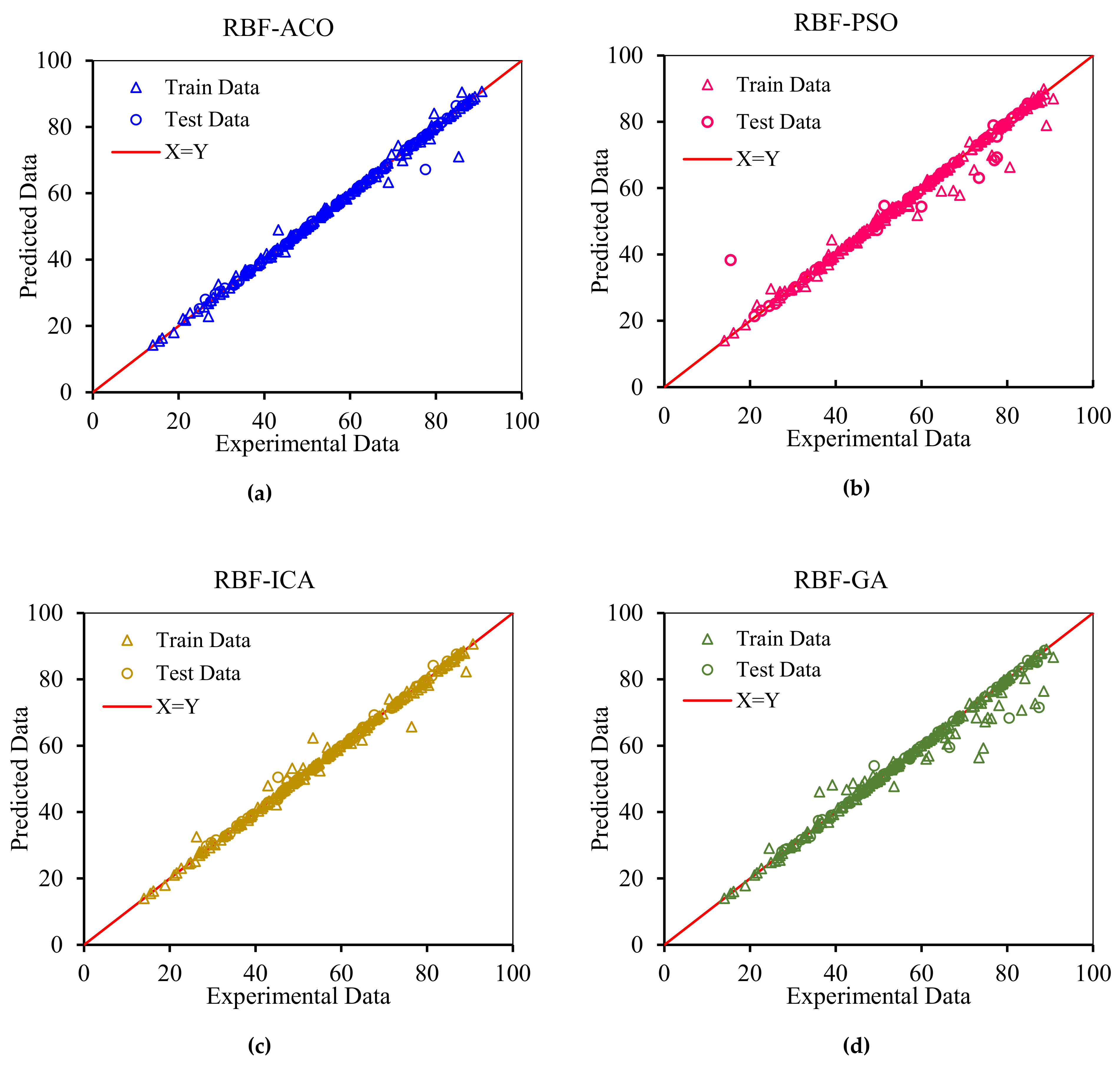
| RBF-ACO | Train | −0.09 | 0.90 | 1.39 | 0.9937 | 0.00061 | 120 |
| Test | −0.03 | 0.84 | 1.53 | 0.9939 | 0.00053 | ||
| Total | −0.08 | 0.89 | 1.42 | 0.9937 | 0.00059 | ||
| LSSVM-CSA | Train | −0.07 | 0.95 | 0.67 | 0.9986 | 0.00018 | 20 |
| Test | −0.25 | 0.91 | 0.64 | 0.9988 | 0.00013 | ||
| Total | −0.11 | 0.94 | 0.66 | 0.9986 | 0.00017 | ||
| MLP-BR | Train | −0.01 | 0.95 | 0.62 | 0.9989 | 0.00013 | 15 |
| Test | −0.21 | 1.34 | 1.00 | 0.9963 | 0.00039 | ||
| Total | −0.10 | 1.04 | 0.72 | 0.9984 | 0.00023 | ||
| MLP-LM | Train | −0.07 | 0.83 | 0.56 | 0.999 | 0.00010 | 10 |
| Test | 0.65 | 2.08 | 1.22 | 0.9963 | 0.00064 | ||
| Total | 0.017 | 1.19 | 0.85 | 0.9978 | 0.00045 | ||
| RBF-ICA | Train | −0.49 | 1.27 | 4.01 | 0.9536 | 0.00300 | 165 |
| Test | −0.63 | 0.92 | 0.99 | 0.9972 | 8.96E-05 | ||
| Total | −0.52 | 1.20 | 3.61 | 0.9618 | 0.00249 | ||
| MLP-SCG | Train | −0.02 | 1.07 | 0.73 | 0.9983 | 0.00017 | 10 |
| Test | 0.34 | 1.73 | 1.04 | 0.9972 | 0.00045 | ||
| Total | −0.07 | 1.30 | 0.87 | 0.9977 | 0.00041 | ||
| MLP-CGF | Train | −0.07 | 1.31 | 0.83 | 0.9977 | 0.00023 | 15 |
| Test | 0.69 | 2.36 | 1.37 | 0.9953 | 0.00077 | ||
| Total | 0.15 | 1.68 | 1.30 | 0.9948 | 0.00072 | ||
| RBF-GA | Train | 0.50 | 1.90 | 2.9 | 0.9753 | 0.00225 | 180 |
| Test | 0.57 | 1.66 | 3.10 | 0.9745 | 0.00170 | ||
| Total | 0.51 | 1.85 | 2.94 | 0.9752 | 0.00214 | ||
| RBF-PSO | Train | 0.28 | 1.42 | 2.01 | 0.9861 | 0.00119 | 220 |
| Test | −2.29 | 4.95 | 4.29 | 0.9628 | 0.04571 | ||
| Total | −0.18 | 2.05 | 2.55 | 0.9805 | 0.00988 | ||
| GMDH | Train | −0.14 | 2.84 | 1.92 | 0.9863 | 0.00167 | 20 |
| Test | −0.26 | 2.66 | 1.95 | 0.9819 | 0.00120 | ||
| Total | −0.17 | 2.81 | 1.92 | 0.9853 | 0.00157 |
© 2020 by the authors. Licensee MDPI, Basel, Switzerland. This article is an open access article distributed under the terms and conditions of the Creative Commons Attribution (CC BY) license (http://creativecommons.org/licenses/by/4.0/).
Share and Cite
Mazloom, M.S.; Rezaei, F.; Hemmati-Sarapardeh, A.; Husein, M.M.; Zendehboudi, S.; Bemani, A. Artificial Intelligence Based Methods for Asphaltenes Adsorption by Nanocomposites: Application of Group Method of Data Handling, Least Squares Support Vector Machine, and Artificial Neural Networks. Nanomaterials 2020, 10, 890. https://doi.org/10.3390/nano10050890
Mazloom MS, Rezaei F, Hemmati-Sarapardeh A, Husein MM, Zendehboudi S, Bemani A. Artificial Intelligence Based Methods for Asphaltenes Adsorption by Nanocomposites: Application of Group Method of Data Handling, Least Squares Support Vector Machine, and Artificial Neural Networks. Nanomaterials. 2020; 10(5):890. https://doi.org/10.3390/nano10050890
Chicago/Turabian StyleMazloom, Mohammad Sadegh, Farzaneh Rezaei, Abdolhossein Hemmati-Sarapardeh, Maen M. Husein, Sohrab Zendehboudi, and Amin Bemani. 2020. "Artificial Intelligence Based Methods for Asphaltenes Adsorption by Nanocomposites: Application of Group Method of Data Handling, Least Squares Support Vector Machine, and Artificial Neural Networks" Nanomaterials 10, no. 5: 890. https://doi.org/10.3390/nano10050890