Joint MT and Gravity Inversion Using Structural Constraints: A Case Study from the Linjiang Copper Mining Area, Jilin, China


1
College of Geo-Exploration Sciences and Technology, Jilin University, Changchun 130026, China
2
Changchun Institute of Technology, Changchun 130021, China
*
Authors to whom correspondence should be addressed.
Minerals 2019, 9(7), 407; https://doi.org/10.3390/min9070407
Submission received: 30 May 2019
/
Revised: 27 June 2019
/
Accepted: 29 June 2019
/
Published: 2 July 2019
(This article belongs to the Special Issue Novel Methods and Applications for Mineral Exploration)
Abstract
:We present a joint 2D inversion approach for magnetotelluric (MT) and gravity data with elastic-net regularization and cross-gradient constraints. We describe the main features of the approach and verify the inversion results against a synthetic model. The results indicate that the best fit solution using the L2 is overly smooth, while the best fit solution for the L1 norm is too sparse. However, the elastic-net regularization method, a convex combination term of L2 norm and L1 norm, can not only enforce the stability to preserve local smoothness, but can also enforce the sparsity to preserve sharp boundaries. Cross-gradient constraints lead to models with close structural resemblance and improve the estimates of the resistivity and density of the synthetic dataset. We apply the novel approach to field datasets from a copper mining area in the northeast of China. Our results show that the method can generate much more detail and a sharper boundary as well as better depth resolution. Relative to the existing solution, the large area divergence phenomenon under the anomalous bodies is eliminated, and the fine anomalous bodies boundary appeared in the smooth region. This method can provide important technical support for detecting deep concealed deposits.
1. Introduction
Many inverse problems in geophysics are ill-posed and the solutions may be non-unique due to errors inherent in the observational data, limitations in the range of observations, the discretization of the observation data, and the simplification of the underground model. Additionally, constraints are often incorporated into the inversion to seek stable solutions. The penalty function regularization technique is one of the most commonly used, where the fundamental idea is that some prior constraints are added to the least-squares misfit term to preserve the stability of the inversion solution [1,2,3].
Different types of penalty functions can be employed in geophysical inversion. The L2 norm regularization imposing smoothness priors is one of the most successful methods [4,5,6,7,8]. This regularization improves the stability of the inversion at the expense of its resolution: the inversion results overestimate the size of the source and blur the boundaries of buried geological contacts as well as their associated physical properties. The total variation (TV) regularization method is a filter to decrease the noise in the data [9,10,11,12] given that a dataset denoised by TV-denoising tends to contain blocks with a constant gray level, separated by intensity gaps, even in what should be smooth areas (the so-called “staircase effect”) [13]. The focusing regularization can obtain focused reconstruction images and even sharper boundaries than the conventional smooth stabilizer. However, if the inversion is over-focused, it sometimes distorts the structural form and makes the inversion result inaccurate. In recent years, with the continuous development of compressive sensing theory and related algorithms, the sparse regularization method has been widely used in many fields, such as signal processing, image denoising, magnetic resonance imaging, and geophysical inversion [14,15,16,17]. This regularization mainly obtains the sub-surface non-zero element, and the response produced by the non-zero element must fit the observed data. The minimization of the L0 norm is a non-deterministic polynomial-time hard problem (NP-hard), which indicates that the optimization algorithms used to solve the problem cannot be completed in polynomial terms [18]. Thus, the L1 norm is usually used to approximate the L0 norm to solve the NP-hard problem. It can be seen that L1 norm regularization has received considerable interest in solving inversion problems [19,20,21,22] and can efficiently capture the small-scale details of the inversion solution. Although L1 norm regularization has shown success in some situation, it has some limitations. When the correlation of a set of variables is very high, L1 norm regularization often only selects one variable and does not care whether another variable is selected. That is, group selection is not possible [23]. Zou and Hastie [24] proposed a new regularization method named the elastic-net regularization method. Elastic-net regularization not only has the advantage of L1 norm regularization, but also takes into account the ability to select groups of related variables and can retain the characteristic variables of the data as much as possible. Elastic-net regularization has been extensively applied in statistics, computer science, and medical imaging, but has not been applied in geophysical inversion [25,26,27].
Each geophysical method has a different resolution and only reflects one physical property of the underground; thus, separate inversion methods have some limitations. Methods to overcome such problems in geophysical inversion are the focus of much research in the inversion community [28]. Currently, the most effective comprehensive interpretation method is joint inversion, and joint inversion can reduce the multi-solution of inversion. The study of integrating multiple data for geophysical exploration can be classified into two categories. The first category is based on coupling the empirical relationships between different physical properties, e.g., fluid saturation and porosity [29,30,31,32]. Unfortunately, this method has some limitations: the lithology of different zones differs, and it is difficult to find the exact relationship between the various physical properties to produce a single relationship.
The second category utilizes structural coupling, which is not dependent on the petrophysics and depends on the similarity of the spatial structure of different physical models to the coupling data as has been reported [33,34,35,36,37,38,39,40]. Gallardo and Meju [33] first published the cross-gradient function, which is used to identify the structure boundary as the cross product between different physical gradients. They reported on a two-dimensional cross-gradient joint inversion study of the seismic time and the direct current (DC) resistivity that achieved good results. Moorkamp [41] compared the results of a petrophysics constrained inversion and a cross-gradient joint inversion of gravity, magnetotelluric (MT), and seismic data. Gallardo et al. [42] first applied the cross-gradients joint inversion algorithm of four methods—namely, gravity, magnetic, MT, and seismic reflection data. Other applications of the cross-gradient approach include integrating ground-penetrating radar travel-time data, cross-hole electrical resistance data, and seismic travel-time data for the better determination of lithologic boundaries in hydrogeologic studies [43,44]. Zhdanov et al. [45] developed a generalized approach to joint inversion based on Gramian constraints by using the formalism of Gramian determinants, which when applied to the parameters’ gradients reduces to a constraint similar to cross-gradients. Haber and Gazit [46] proposed a novel approach based on a joint total variation function. The joint total variation is a convex function for joint inversion and can improve the inversion of models with a sharp interface. The above structural coupling joint inversion mainly uses a separate smooth or focusing regularization method and rarely uses a hybrid regularization method. The obtained inversion results may be too smooth or too sparse, affecting the accuracy of the inversion results. Furthermore, the cross-gradient constraint proposed above is directly structurally coupled through model parameters. Since there are different units and magnitudes between different physical parameters, direct coupling may affect the inversion results. To address these issues, we first investigated an elastic-net regularization method as a convex combination term of the L2 norm and L1 norm can not only enforce the stability to preserve large-scale smoothness, but can also efficiently capture the small-scale details of the inversion solution and enforce the sparsity to preserve sharp boundaries. Next, we considered whether the normalization method could effectively eliminate large differences in magnitude between the model parameters.
In this paper, we present an original approach to the joint inversion of MT and gravity data based on elastic-net regularization and cross-gradient constraints. Considering the fact that the L2 norm penalty always makes the inversion results overly smooth and the L1 norm penalty always makes the inversion results too sparse, we investigated an elastic-net regularization method with a stronger convex combination of the L1 norm and the L2 norm for an ill-posed joint inversion problem. We constructed a new joint inversion penalty function, that is, based on the data misfit terms, we added L1 norm and L2 norm regularization to form an elastic-net regularization. The elastic-net regularization can effectively improve the blur degree of the L2 inversion result and the over-sparse degree of the L1 norm inversion result, so that the inversion is not only stable, but can also enforce the sparsity to preserve sharp boundaries. We used synthetic models of the subsurface to gauge the performance of the algorithm and test its accuracy. Then, we applied this approach to the interpretation of geophysical field data collected in the Linjiang (Jilin Province) copper mining area in Northeast China.
2. Joint Inversion Methodology
To avoid the instability and multi-solution problems caused by solving ill-posed inverse problems, the Tikhonov regularization method is used to solve linear equations. We constructed the joint inversion objective function of MT and gravity data, which is expressed as follows:
where, is represented as a data misfit term; is represented as a model constraint term; and is a regularization factor. (apparent resistivity and phase) and (gravity Bouguer anomaly) are the observed data. are the computed apparent resistivities and phases and is the computed gravity Bouguer anomaly. and are the vectors of resistivity and density, respectively. and are the prior model of resistivity and density, respectively. and are represented as the MT and gravity regularization factor, respectively. and are the noise error diagonal inverse matrix of the MT and gravity data, respectively. and are the MT and gravity model weighting matrix where the smooth roughness model matrix is usually adopted, respectively. is the cross-gradient constraint term. A convenient un-normalized way to measure the geometrical similarity of the models can be obtained through the use of the cross-gradient function [33,34] given by
where and are the resistivity and density property gradients, respectively. Please note that resistivity and density have different orders of magnitude and units. If the physical parameter gradients are directly coupled, it may produce inaccurate inversion results. In this paper, we added a normalized factor to the cross-gradient constraints term to overcome the effects of different physical parameter differences. The cross-gradient constraints term expression that is added to the normalized factor is as follows:
where and are the normalized operators of resistivity and density, respectively. The normalized operator is determined by the amount of change in the model parameters of the separate inversion results.
Our objective function (1) is nonlinear, since the MT forward problem and the cross-gradient constraints are nonlinear. Our solution to Equation (1) is thus achieved by linearization. For the MT forward problem, we computed forward responses using the OCCAM2DMT code developed by deGroot-Hedlin and Constable [47], which uses the FE forward modeling code developed by Wannamaker [48]. For the gravity forward problem, we used analytical solutions for polygonal prisms [49]. The nonlinear problem was transformed into a linear problem by using a first-order Taylor expansion (neglecting higher orders), namely,
where A1 defines the resistivity Jacobian matrix, which calculates the Jacobian matrix using reciprocity. A2 defines the density Jacobian matrix. and are the initial models of resistivity and density, respectively.
Similarly, the linearization of the cross-gradient constraints in Equation (3) can be accomplished by using a first-order Taylor expansion (neglecting higher orders), namely,
where the derivative of for the model parameters is given by B.
Using Equations (4)–(6), the linearized equivalent of Equation (1) is stated as
For convenience, we introduced an integrated model parameter and an integrated data parameter . Then, the objective function in Equation (7) can be rewritten as
where ; ; ; ; ; ; and .
The solution of Equation (8) can be determined using Lagrange multipliers [50], by solving the system of equations:
The solutions to Equations (9) and (10), after some algebra, are
where ; .
Equation (12) is used as a model update expression, where the first term on the right side of Equation (12) corresponds to the regularized least squares solution (no cross-gradient constraints), whereas the second term corresponds to the structural constraints solution.
3. Regularization Inversion Methodology
To reconstruct the stable inversion model, some sort of regularization model constraints are required. Regularization model constraints come in numerous forms, that is, in Equation (8) can choose different forms. Different inversion methods can be developed by changing the model constraints such as smooth inversion based on the L2 norm, sparse inversion based on the L1 norm as well as focusing inversion and total variation inversion, and so on. Below, we discuss the principles and characteristics of these inversion methods.
3.1. L2 Norm Regularization
The L2 norm defined by refers to the square root of the squares of the elements in the vector. The self-multiplication of each element in the L2 norm means that the element with a large value contributes a large amount to the whole, thus minimizing the L2 norm of a model produces a relatively smoothly changing model. Occam inversion is also essentially an inversion based on the L2 norm inversion. Its model constraint represents the difference of adjacent element model parameters. Minimizing the model constraint causes the difference in the adjacent element model parameters to be minimized, so the inversion result is smooth. In this paper, the L2 norm inversion used the same model constraints as the Occam inversion. The expression of the L2 norm regularization term for a 2D model is as follows
where is a roughening matrix that differences the model parameters of laterally adjacent elements, and is a roughening matrix that differences the model parameters of vertically adjacent elements. is a gradient operator. The details of the roughening matrix mathematical expression can be found in deGroot-Hedin [47]. Equation (14) is brought into Equation (12) to obtain a model update based on the L2 norm.
3.2. L1 Norm Regularization
The L1 norm defined by refers to the sum of the absolute values of the elements in the vector and is also known as the sparse operator. The introduction of the sparse operator can remove the features without information in the inversion, that is, the weight corresponding to these features is set to zero. The feature with information corresponds to the anomalous area of the underground medium, while the feature without corresponds to the background area of the underground medium. Therefore, sparseness highlights the distribution features of subsurface anomalies. The model solution of the sharp boundary can be obtained by inversion based on the L1 norm. The expression of the L1 norm regularization term is as follows
To avoid singularity in the case of m = 0, the L1 norm regularization of the model is generally approximated by
where is a small number, so we set . A possible method for solving Equation (16) is to approximate the L1 norm minimization as an iteratively reweighted L2 norm minimization problem [51,52,53].
Equation (18) is brought into Equation (12) to obtain a model update based on the L1 norm.
3.3. Focusing Regularization
Last and Kubic [54] proposed a minimum support function (MS) as a model constraint, which can minimize the section area of the anomalous body. The expression of the minimum support function can be expressed as:
where e is a focusing parameter determining the sharpness of the produced image [55]. Inversion based on focusing regularization can recover a model with clearer boundaries and contrasts than the traditional smooth inversion. However, it tends to produce the minimum volume of a model, which usually underestimates the distribution space of the recovered model. Equation (20) is brought into Equation (12) to obtain a model update based on the focusing regularization.
3.4. Total Variation Regularization
The total variation regularization method was first proposed as an image denoising technique for image processing [56]. It uses a variation function as a penalty function and belongs to a class of bounded variation function, which allows discontinuous points. The total variation method can effectively reconstruct non-smooth images with “corner points”, that is, the case of a discontinuous solution, and has better edge preservation. However, the main disadvantage is that the reconstruction results often show a blocking phenomenon, which is prone to the “staircase effect”. The total variation function is defined as
Various approaches can be used to approximate the original TV term to make it differentiable at the origin. One common approach to make the original TV term differentiable is to introduce a small smoothing parameter such that
Equation (25) is brought into Equation (12) to obtain a model update based on the TV regularization.
3.5. Elastic-Net Regularization
Zou and Hastie [24] proposed a new regularization method named the elastic-net regularization method. The elastic-net regularization method, a convex combination term of the L2 norm and L1 norms, can not only enforce the stability to preserve large-scale smoothness, but can also efficiently capture the small-scale details of the inversion solution and enforce the sparsity to preserve sharp boundaries. It is similar to a stretchable fishing net that retains “all the big fish”. This method has been extensively applied in statistics, computer science, and medical imaging, but is rarely used in geophysical inversion. Elastic-net regularization is defined as
where and are the non-negative parameters used to control the relative weighting of the L1 norm and the L2 norm. Let be a convex combination regularization term equal to Equation (26) can be expressed as
The regularization term (Equation (27)) reduces to L2 norm regularization, while the regularization term (Equation (27)) reduces to L1 norm regularization. In this paper, we assigned a non-zero value for (i.e., ), since we wanted to emphasize the structural features of sparsity for all iterations. This will typically reduce overly smooth behavior while well maintaining the sharp edges. Equation (29) is brought into Equation (12) to obtain a model update based on the elastic-net regularization. Please note that gravity inversion requires model weighting matrices. In this paper, the model weighting functions were based on the depth-weighting function used to counteract the depth-dependent decay of the sensitivity matrix. When denoting the model weighting function as Z, Wm is replaced by diag(Z)·Wm in all of the above equations.
4. Synthetic Example
4.1. Comparison Regularization Methods
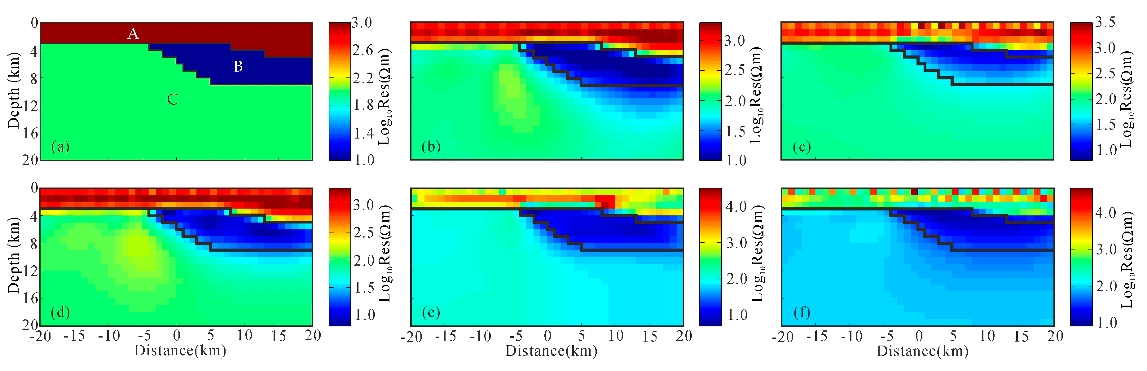
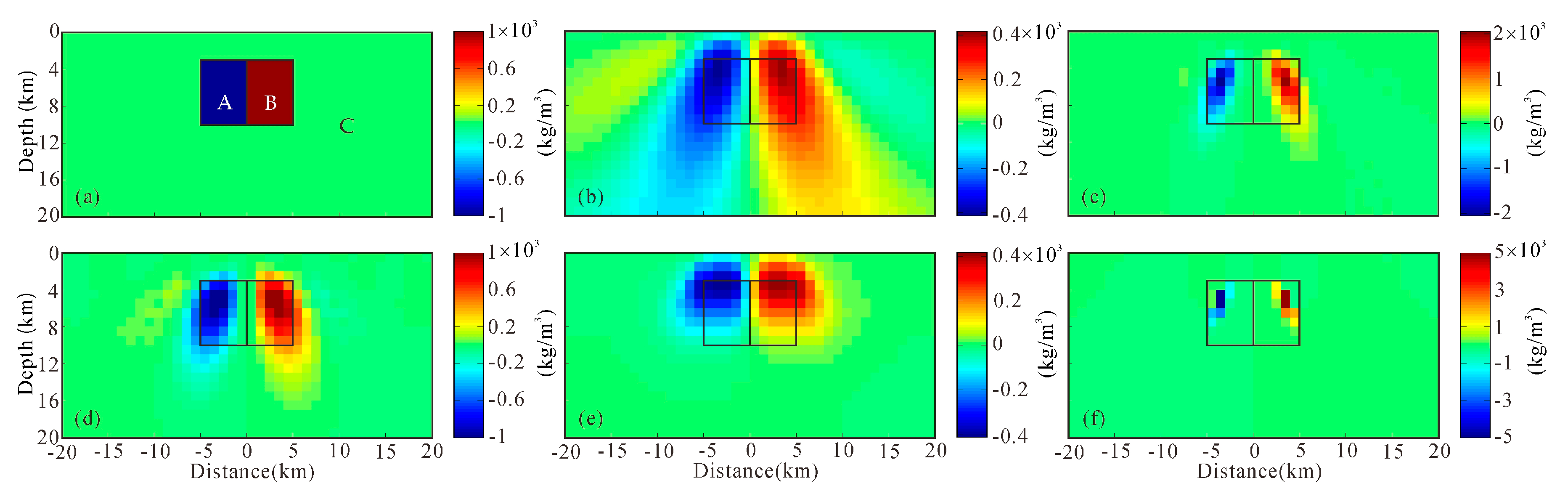
To illustrate the feasibility and efficiency of the elastic-net regularization method, we inverted the MT and gravity data using different regularization methods by different typical resistivity and density synthetic models, as shown in Figure 1a and Figure 2a. The physical property values of the resistivity and residual density models are listed in Table 1. The resistivity model features a conductive wedge underlying a highly resistive surface layer and overlying a basement of intermediate resistivity, representative of sediments below basalts. The residual density model consists of adjacent low and high-density blocks in the homogeneous subsurface surrounding rock. For the resistivity model, apparent resistivity and phase data for both the transverse electric (TE) and transverse magnetic (TM) modes were generated at 14 stations, spaced at 3 km intervals. The frequency ranges were chosen so that the penetration depth corresponded to the top unit at the highest frequency and the bottom unit at the lowest frequency (at 10 frequencies from 25 to 0.05 Hz). For the density model, the gravity data were Bouguer corrected at 41 stations spaced uniformly from a horizontal distance −20 km to 20 km. To simulate the noisy data, 5% random Gaussian noise was added to the MT and gravity data prior to inversion. The density model grid was set to 125 × 41 in the horizontal and vertical directions, respectively. However, the resistivity model grid needed to be extended from the density model grid, and the grid size was 141 × 55. The starting model was a homogeneous medium with a resistivity of 100 Ω·m and a residual density of 0 kg/m3.
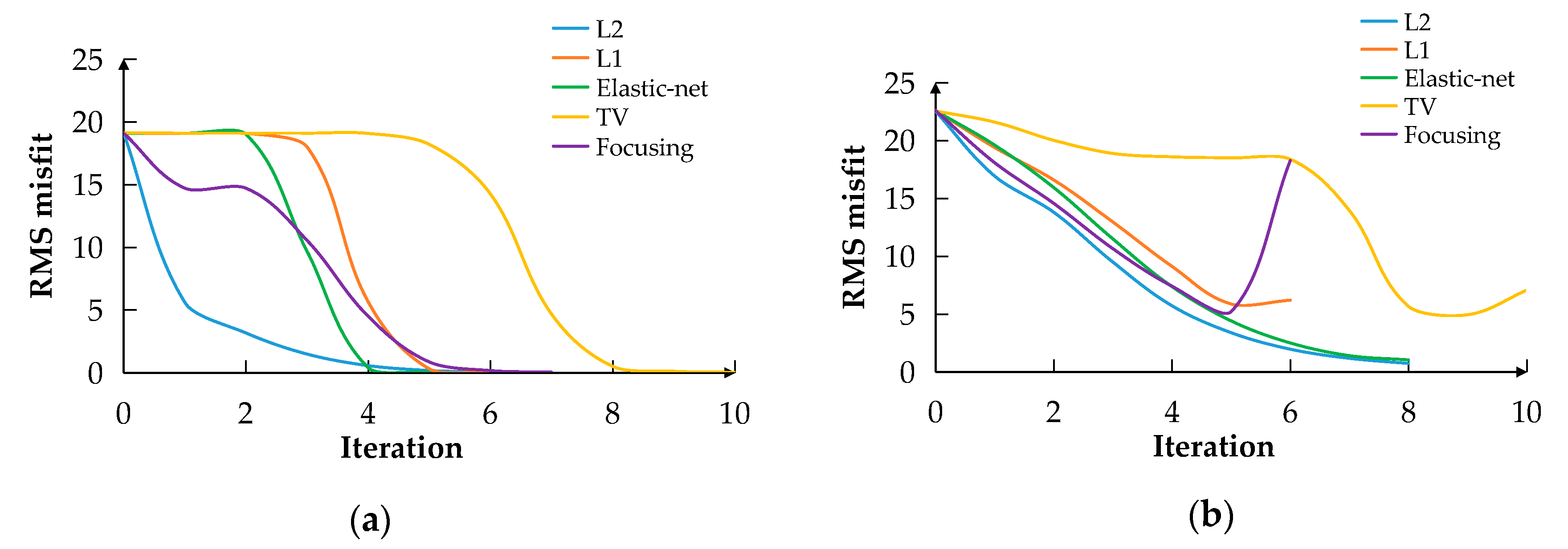
For comparison, we conducted these tests on four other regularization methods: the L2 norm, L1 norm, TV, and focusing, respectively. The best-fitting resistivity models were achieved by five different regularization inversions (Figure 1b–f), the evolution of the RMS misfit at every iteration of the five different regularization inversion processes is shown in Figure 3a. Inversion using the L2 norm regularization yielded a relatively stable and smooth result, as shown in Figure 1b, but the results blurred the wedge sharp boundaries of the subsurface geological contact. The L1 norm regularization method (Figure 1c) exhibited sparse characteristics; the wedge sharp boundaries were inverted, but the inversion convergence was poor, showing some instability, and the anomalous amplitude of recovery was larger than the true model. The TV regularization method could reconstruct non-smooth images, as shown in Figure 1e. However, the inversion result differed from the true model, and the convergence was poor, showing instability. The focusing regularization method seeks the source distribution with the minimum volume. As a result, the inversion result (Figure 1f) was too focused and even provided the wrong wedge boundaries; moreover, the value of resistivity was greater than the amplitude of the true model. A comparison of the solution with the true wedge sharp shown superimposed on the model indicated that both the unit conductivities and boundary locations had been well imaged (Figure 1d). In particular, the shape of both the top and low wedge boundaries were well recovered within the limits afforded by the stairstep approximation. The elastic-net regularization method could not only enforce the stability to preserve large-scale smoothness, but also efficiently enforced the sparsity to preserve sharp boundaries.
The best-fitting density models were achieved by five different regularization inversions (Figure 2b–f); the evolution of the RMS misfit at every iteration of the five different regularization inversion processes is shown in Figure 3b. Inversion using the L2 norm regularization yielded a relatively stable and smooth result, which revealed a large area of ambiguous divergence, and it was difficult to identify the deep boundary of anomalous bodies, as shown in Figure 2b. The L1 norm regularization method inversion results underestimated the size of anomalous bodies, and the gravity inversion obtained a physical property value of anomalous bodies that was larger than the true model, as illustrated in Figure 2c. The TV regularization method inversion result could reconstruct block images, but the center of the anomalous body moved up, as shown in Figure 2e. The anomalous body recovered from the focusing regularization was too focused and it severely underestimated the size of the anomaly, and even provided the wrong model boundaries, as shown in Figure 2f. The elastic-net regularization inversion (Figure 2d) could effectively improve the blur degree of the L2 inversion result and the over-sparse degree of the L1 norm inversion result, so the inversion was not only stable, but also could enforce the sparsity to preserve sharp boundaries.
4.2. Comparison Separate and Joint Inversion
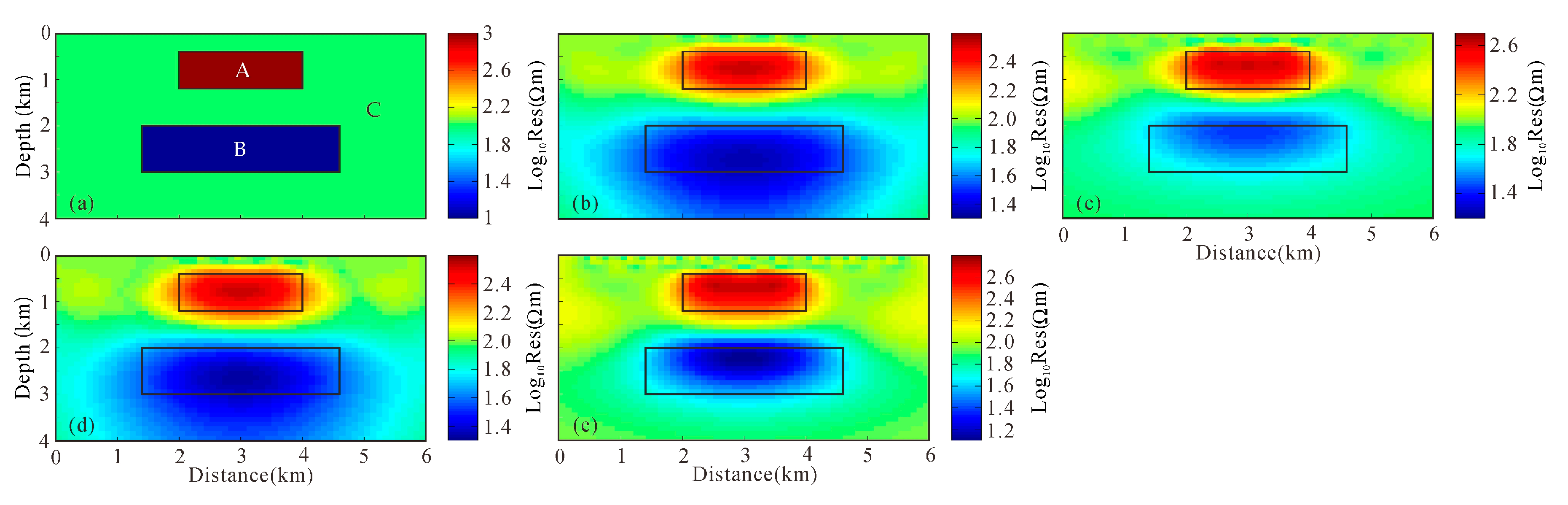
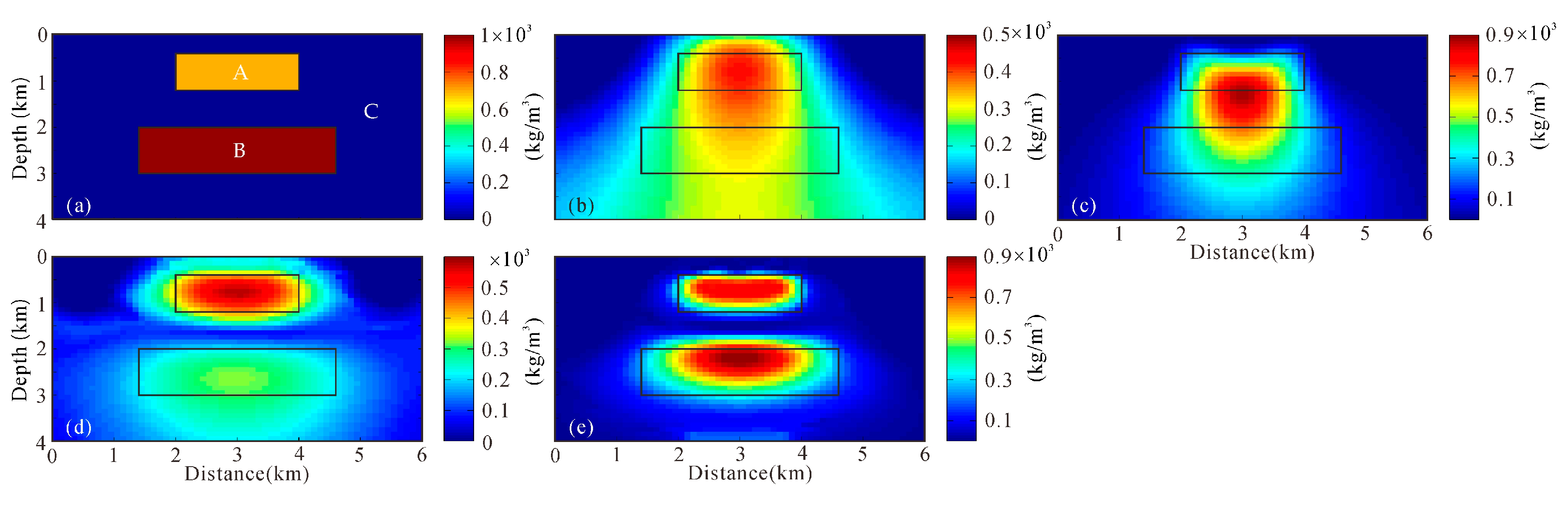
In this section, we explore the advantages of the elastic-net regularization joint inversion compared to separate inversion and traditional joint inversion using an upper and lower anomalous bodies model, as shown in Figure 4a and Figure 5a. The physical property values of the resistivity and residual density models are listed in Table 2. For the resistivity model, apparent resistivity and phase data for both the transverse electric (TE) and transverse magnetic (TM) modes were generated at nine stations, spaced at 0.6 km intervals. The frequency ranges were chosen so that the penetration depth corresponded to the top unit at the highest frequency and the bottom unit at the lowest frequency (at 10 frequencies from 1000 to 1 Hz). For the density model, the gravity data were Bouguer corrected at 30 stations spaced uniformly from a horizontal distance 0 km to 6 km. To simulate noisy data, 5% random Gaussian noise was added to the MT and gravity data before inversion. The density model grid was set to 141 × 81 in the horizontal and vertical directions, respectively. However, the resistivity model grid needed to be extended from the density model grid, and the grid size was 157 × 95. The starting model was a homogeneous medium with a resistivity of 100 Ω·m and a residual density of 0 kg/m3.
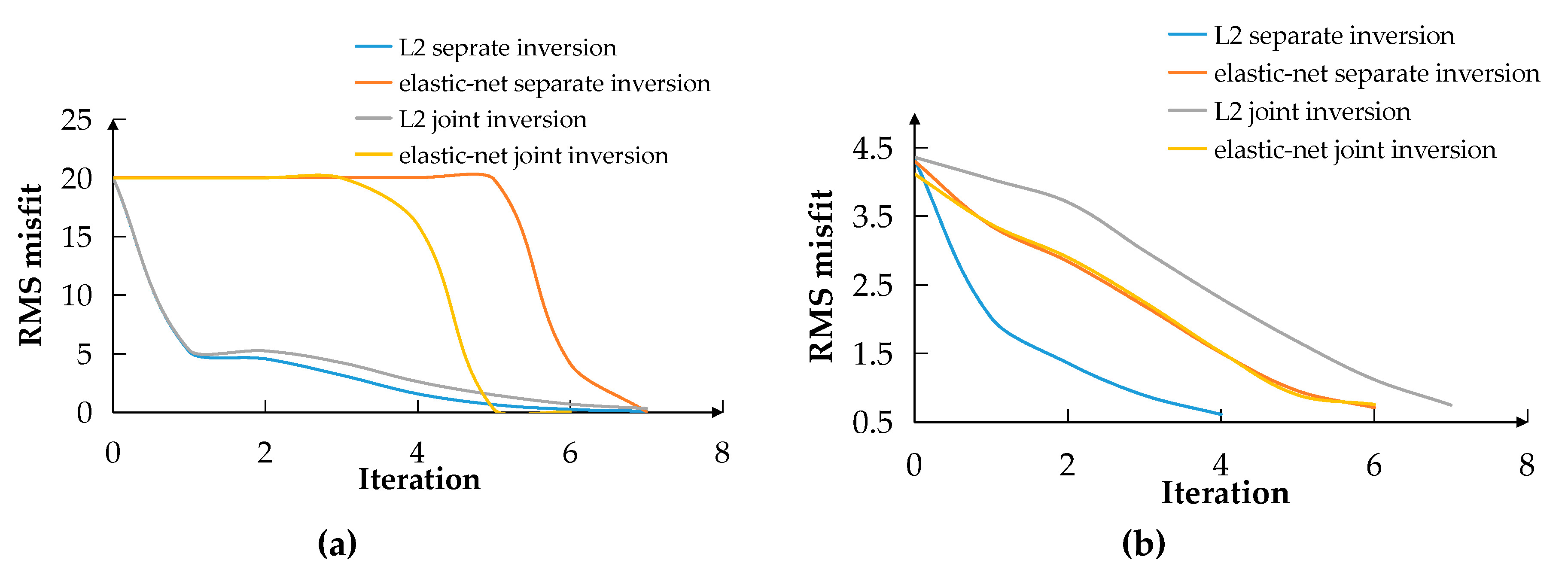
For comparison, we performed these tests on the separate and joint inversion using the L2 and elastic-net regularization methods. The best-fitting resistivity models were achieved by separate and joint inversion using the L2 and elastic-net regularization methods (Figure 4b–e), the evolution of the RMS misfit at every iteration of the inversion process is shown in Figure 6a. Separate and joint inversion of the MT method using the L2 norm regularization yielded a relatively stable and smooth result, as shown in Figure 4b,d, but the results blurred the boundaries of the underground block, in particular, the deep low-resistance block exhibited a serious divergence. Although the MT method in the joint inversion incorporated the structural similarity constraint of the gravity method, the vertical resolution of the gravity was relatively poor, so joint inversion also found it difficult to improve the vertical resolution of the MT method. The elastic-net regularization separate and joint inversion (Figure 4c,e) could effectively improve the blur degree of the deep low-resistance block and more clearly identify the lower boundary of the deep block. Please note that the physical parameters of the block resistivity obtained from the joint inversion of the elastic-net regularization were closer to the true model, which was due to the contribution of the gravity inversion structural similarity constraints.
The best-fitting density models were achieved by separate and joint inversion using the L2 and elastic-net regularization methods (Figure 5b–e), the evolution of the RMS misfit at every iteration of the inversion process is shown in Figure 6b. Separate inversion density models of the L2 and elastic-net regularization methods could not distinguish the upper and lower blocks, showing an anomalous region with high density, as shown in Figure 5b,c. Although the elastic-net regularization was added to the inversion objective function of the gravity, we found that the inversion of the gravity still did not solve the problem of vertical low resolution. Joint inversion density models of the L2 and elastic-net regularization methods (Figure 5d,e) could distinguish the upper and lower blocks as an indirect contribution propagated from the resistivity model by the cross-gradient constraints, showing improved features when compared to the above separate inversion results. Although the density model of the L2 regularization joint inversion (Figure 5d) could identify the upper and lower anomalous blocks, the inversion showed that the high-density anomalous block was above, and the low-density anomalous block was below, which was quite different from the true model. However, in the joint inversion of the elastic-net regularization method (Figure 5e), we found that the boundaries of the anomalous blocks became clearer, and the geometrical and physical values of the anomaly more closely reflected the true model. In particular, the vertical resolution of the density models was significantly improved, and the upper and lower anomalies could be identified as an indirect contribution propagated from the resistivity model by the cross-gradient constraints.
Compared with all of the above inversion methods, the method based on elastic-net joint inversion has its advantages, and not only can it enforce the stability to preserve large-scale smoothness, but it can also efficiently enforce the sparsity to preserve sharp boundaries.
4.3. Noise Effect and Sensitivity Analysis of Elastic-Net Joint Inversion
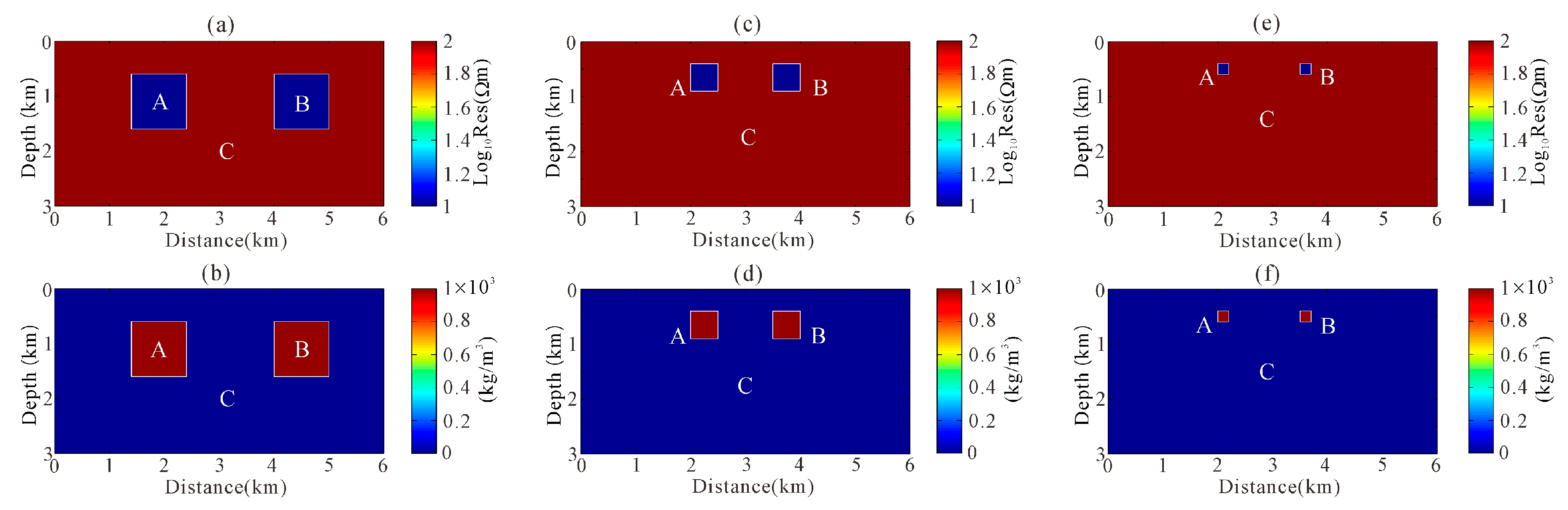
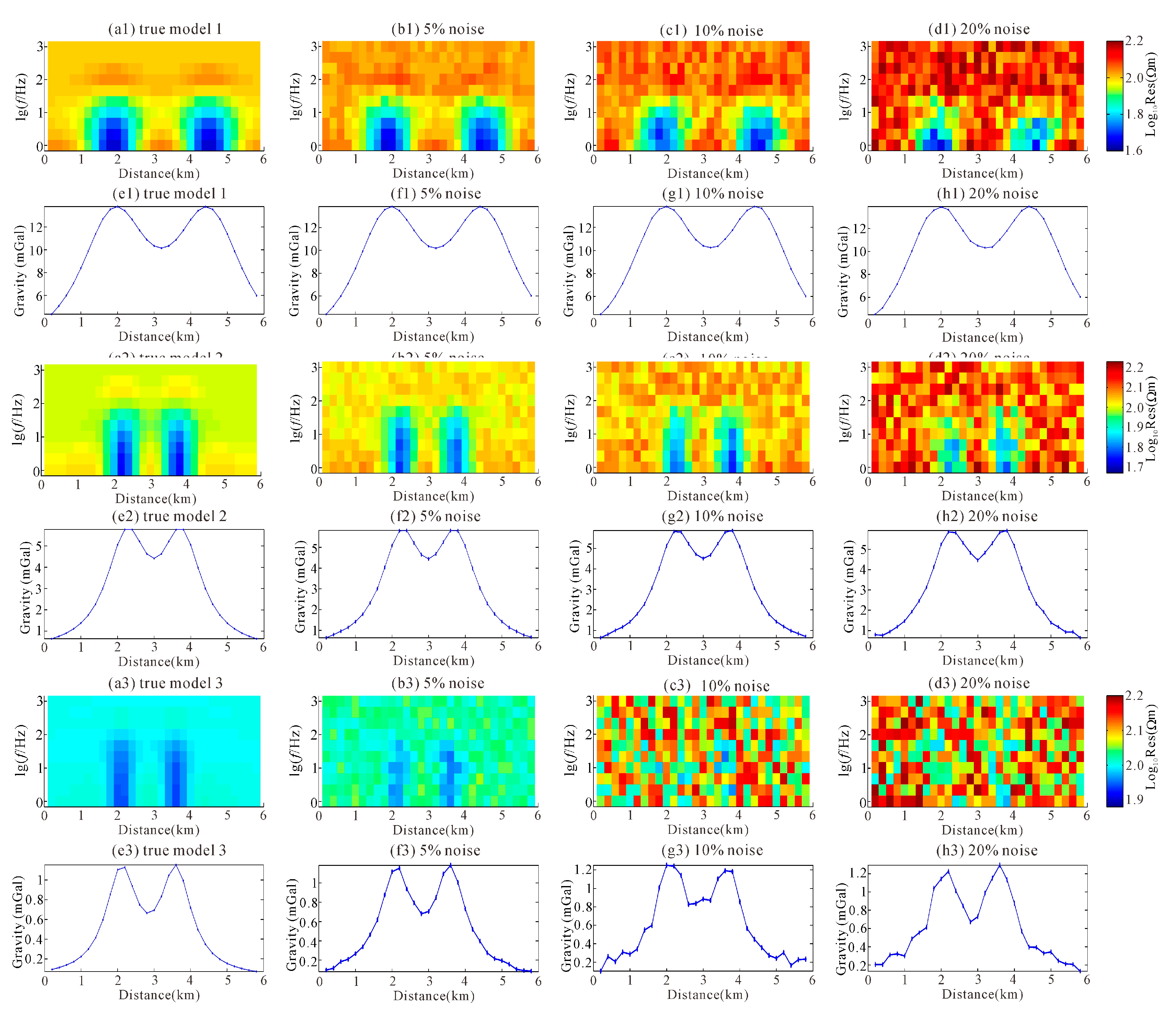
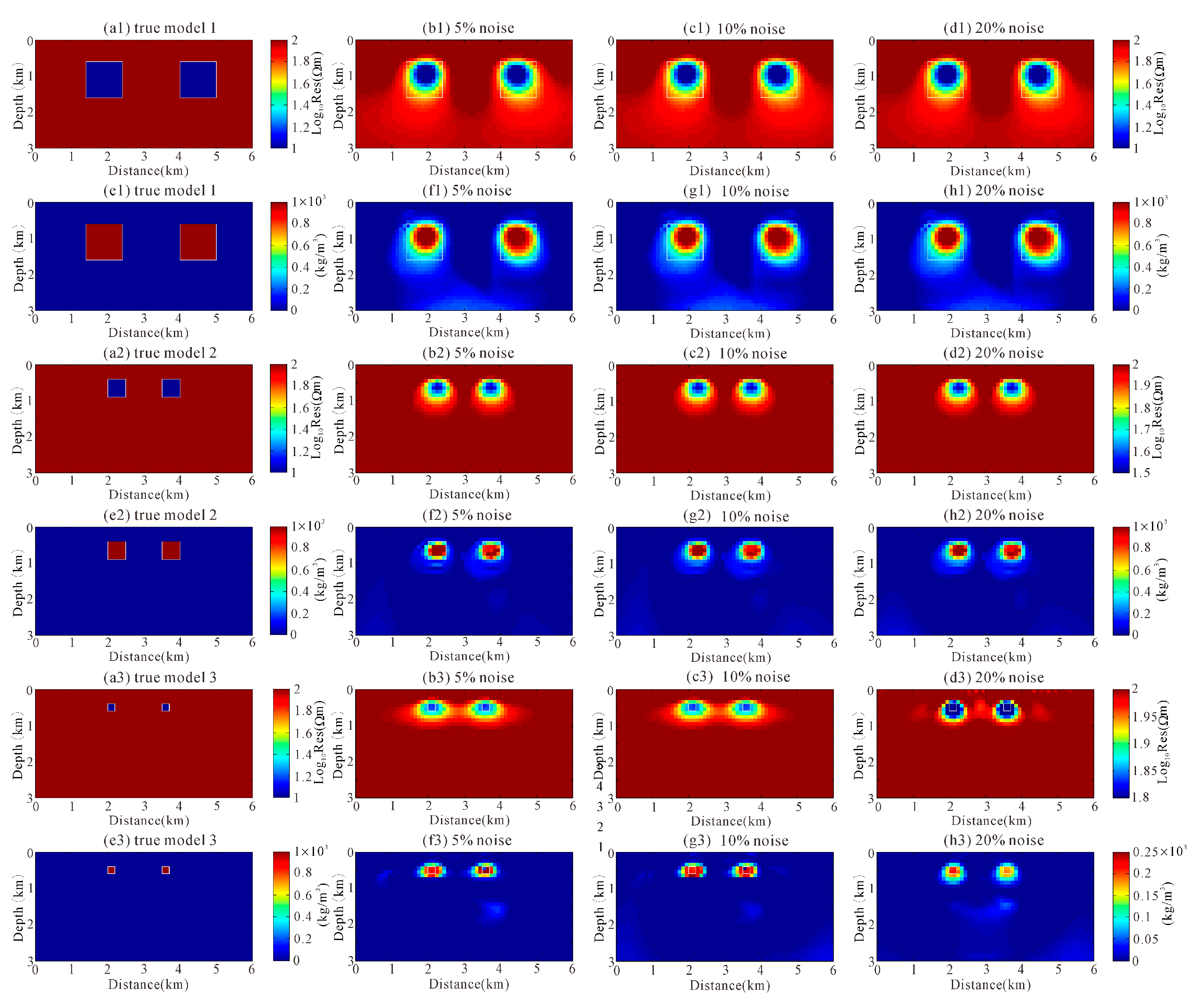
In this section, we tested the impact of noise on the inversion results and analyzed the sensitivity of the inversion method. We designed three models for MT and gravity methods, each with a different source size, as shown in Figure 7a–f. All models included two rectangular boxes of the same size embedded in a half-space. The distribution of the observation points and mesh sizes of all of the models were the same. The physical property values of the resistivity and residual density models are listed in Table 3. For the resistivity model, apparent resistivity for transverse magnetic (TM) mode were generated at 29 stations, spaced at 0.2 km intervals (at 10 frequencies from 1000 to 1 Hz). For the density model, the gravity data were Bouguer corrected at 29 stations spaced uniformly from a horizontal distance 0 km to 6 km. The density model grid was set to 141 × 61 in the horizontal and vertical directions, respectively. The resistivity model grid needed to be extended from the density model grid, and the grid size was 157 × 75. We added 5%, 10%, and 20% random Gaussian noise to the resistivity and density model responses, respectively. The model response results after adding noise are shown in Figure 8. We found that useful signals would be covered by the increase of noise, especially when using the MT method. At the same time, when the anomalous sources became small, the noise may completely cover the useful signals.
We first performed inversion tests on model response datasets with 5%, 10%, and 20% random Gaussian noise, respectively (Figure 9a1,e1). All the starting models were homogeneous medium with a resistivity of 100 Ω·m and a residual density of 0 kg/m3. It was found that the model response datasets after adding noise in model 1 could still recover inversion results similar to the true model, as shown in Figure 9a1–h2. This shows that the inversion method has certain anti-noise ability and is suitable for field measurement data processing with high noise. Next, we performed an inversion sensitivity analysis. We reduced the size of the anomalous sources of the model (Figure 9a2,e2) and added 5%, 10%, and 20% random Gaussian nosie to the theoretical model response. The inversion results showed that when the anomalous sources shrank to 0.5 × 0.5 km2, the inversion method could still recover similar results to the true model. However, when the anomalous sources shrank to 0.2 × 0.2 km2 (Figure 9a3,e3), we found that accurate inversion results might not be obtained with the increase of noise, mainly because the response amplitude of the model was smaller than the noise magnitude, especially the MT method. At this time, our inversion method may not have identified less than 0.2 × 0.2 km2 anomalous sources, so when using this inversion for field data inversion, an anomalous source smaller than 0.2 × 0.2 km2 needs to be interpreted with caution, as it may be a false anomaly. For anomalous sources above 0.2 × 0.2 km2, the inversion could be accurately identified and identified as a true anomalous source.
5. Field Example
5.1. Geologic Background of the Survey Area
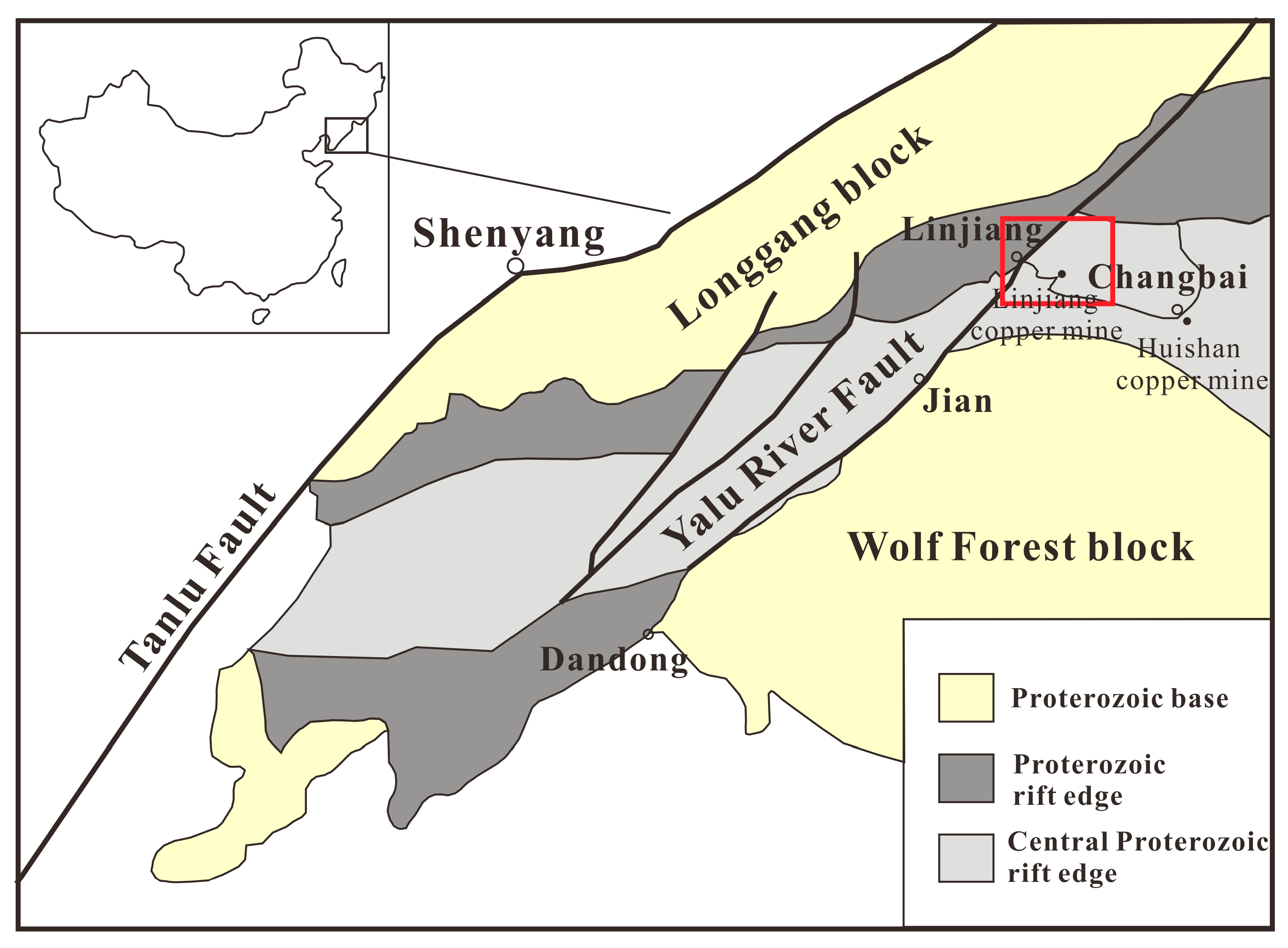
The Linjiang area of Jilin Province is located in the proterozoic Liaoji Rift Valley. The north and south sides are the Wolf Frost block and Longgang block, respectively (Figure 10). The Linjiang copper mine is located in Liudaogou Town, Linjiang City. The exposed strata in the mining area are mainly Laoling group metamorphic rocks, Mesozoic effusion rocks, and Tertiary basalts. The Laoling group stratum is affected by multi-stage tectonic formation, mainly composed of marble and hornstone, and local schist and phyllite. The Mesozoic intrusive rocks are mainly composed of a set of medium-acid volcanic rocks. The formation and distribution of the Linjiang copper deposit are closely controlled by the structure of the area. The ore deposit is located on the north-east side of the deep fault of the Yalu River. The northeastward fault of the main ore body controls the magmatism and mineralization in the mining area. The junction of the north-east fault and the east-west fault intersects and produces the granodiorite body, which controls the distribution of the copper deposit and is the most important ore-conducting structure in the mining area. The magmatic rocks in the mining area are widely distributed and mainly include the Yanshanian hornblende gabbro, the Yanshanian early acid volcanic complex, the Yanshanian mid-granitic granodiorite associated with mineralization, and the re-invasive quartz diorite. Therefore, the Linjiang copper mining area has good metallogenic conditions, large ore-forming intensity, various types of deposits, and potential for finding skarn-type copper deposits in the periphery and deep mining area.
5.2. Data Acquisition
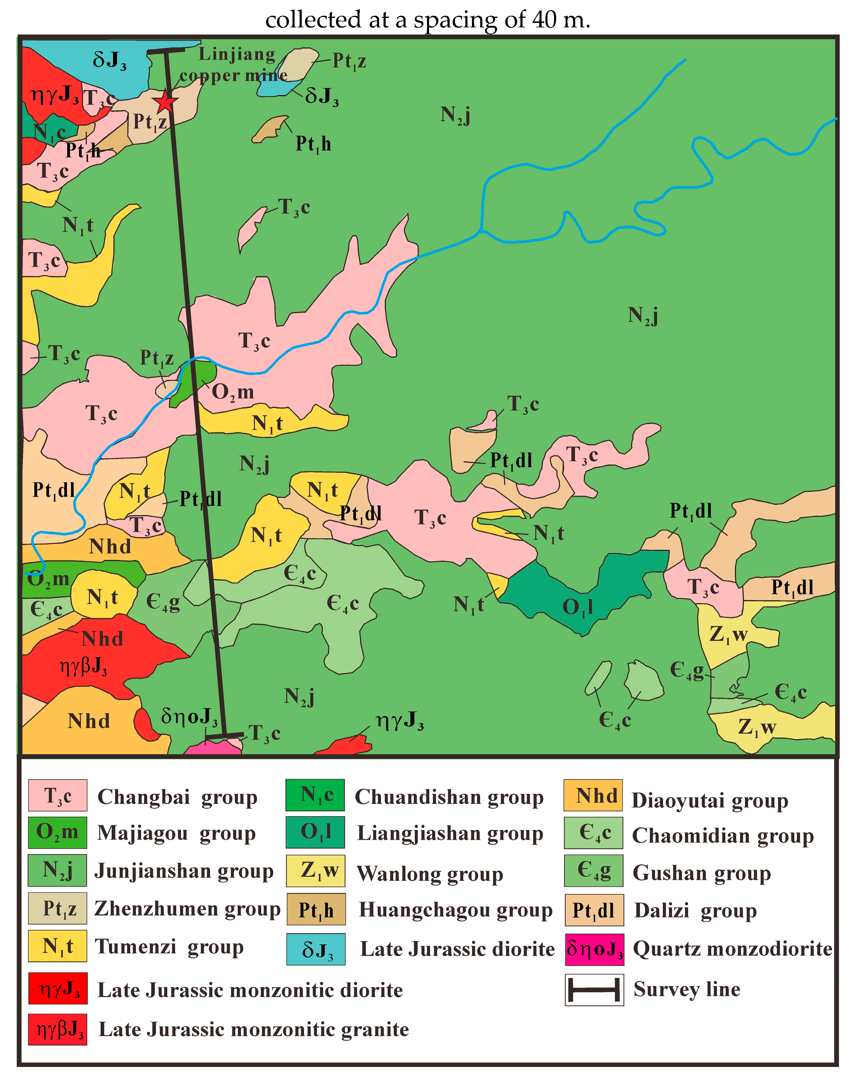
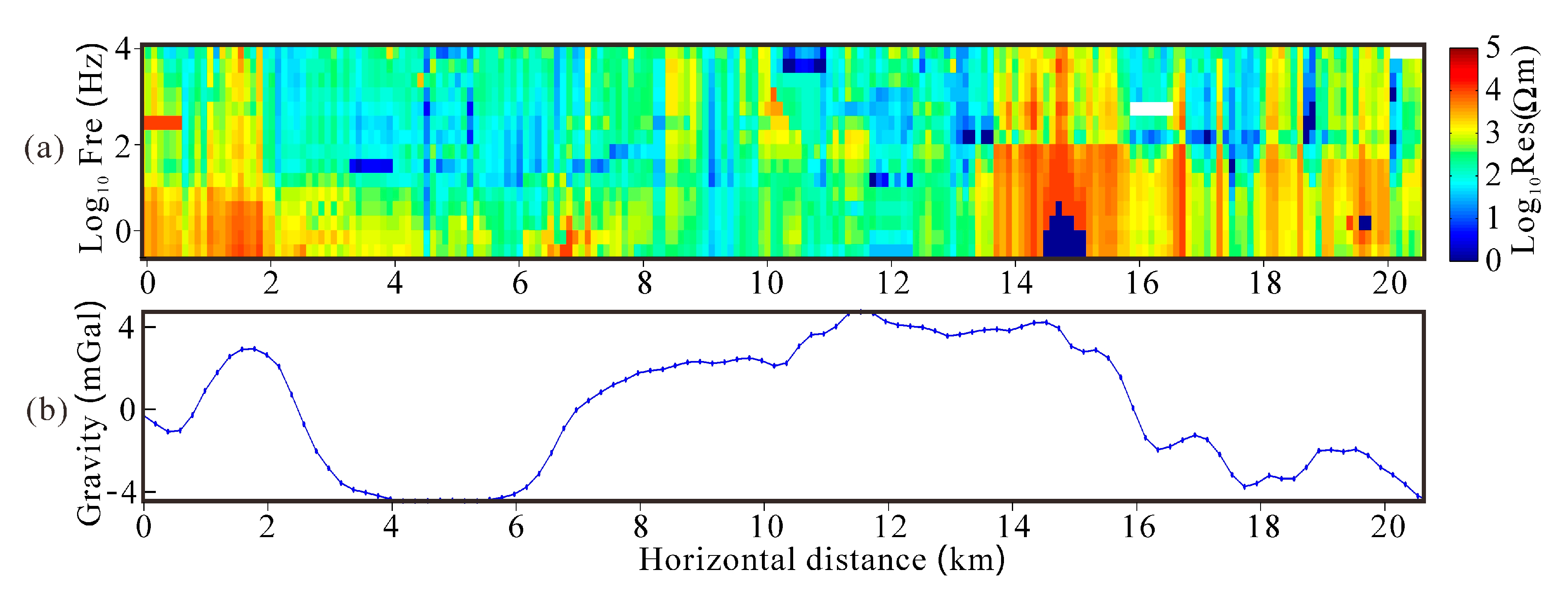
The Linjiang copper mining area is mainly covered by basalts of varying thicknesses and is a semi-concealed deposit. We conducted a geophysical survey along one profile in the study area. Figure 11 shows the geological map of the study area. The black solid line indicates the position of the survey line. The survey line runs in a north-south direction and measures 20.7 km in length. Multiple geophysical surveys, which included CSAMT (controlled-source audio-frequency magnetotelluric) and gravity exploration, were carried out along the survey line. Gravity and CSAMT data were collected along the survey line using a high-precision metal spring gravity meter (Burris, USA) and a GDP-32II (Zonge Company, USA), respectively. A total of 207 CSAMT points were collected at an interval of 100 m and 17 frequencies were collected at each point. The observed data were the apparent resistivity in TM mode (Figure 12a), which were obtained by the full-region apparent resistivity conversion. Furthermore, 526 gravity observation points (Figure 12b) were collected at a spacing of 40 m.
5.3. Inversion Models of CSAMT and Gravity Data
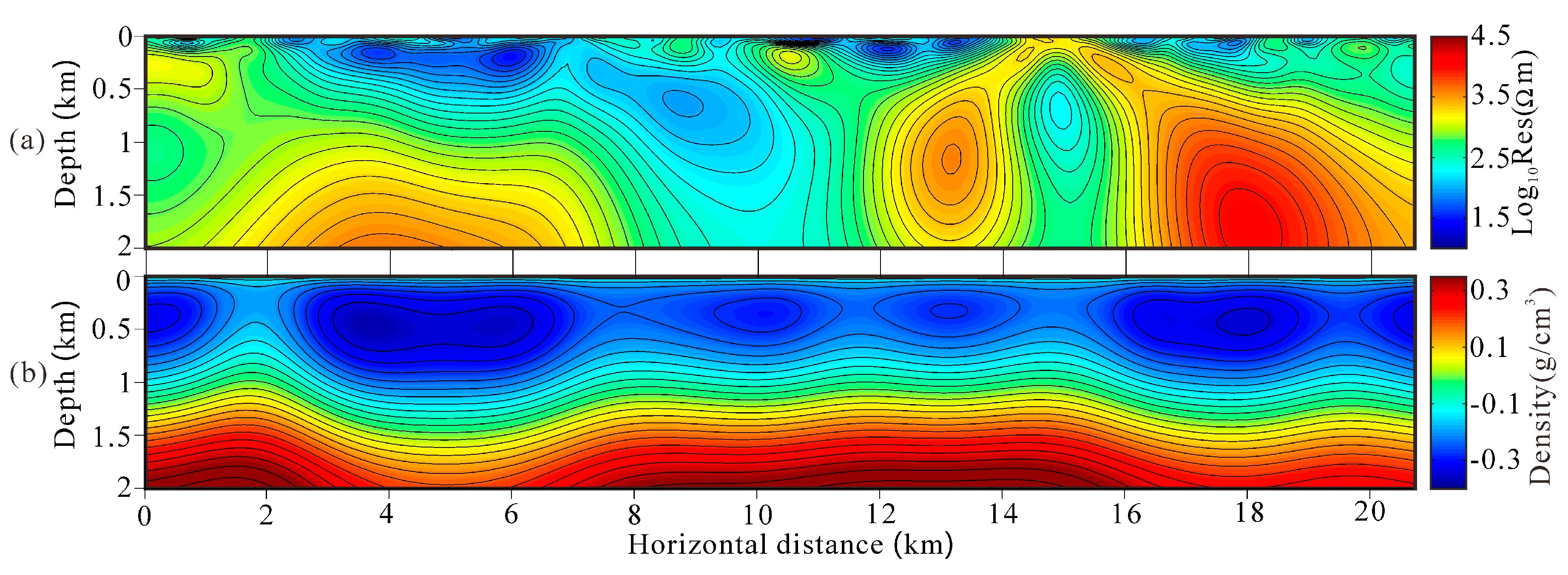
The CSAMT and gravity data were inverted to 2D resistivity and residual density models using separate inversion, joint inversion using smooth regularization method, and joint inversion using the elastic-net regularization method. For our inversion, our base model of the subsurface was discretized on rectangular cells 100 m wide and 10 to 100 m thick. This base model was padded by logarithmically spaced cells beyond its four edges to allow for the decay of the electromagnetic fields. These models were initially assigned homogeneous property values of 102.5 Ω·m, 0.0 kg/m3 in rock formation. The models obtained from the separate inversion are shown in Figure 13. The RMS misfit values found after separate inversion were as follows: RMSCSAMT = 1.39 and RMSGRV = 0.45. The separate inversion models showed major structural differences, and an interpreter will be faced with difficulties in interpreting them.
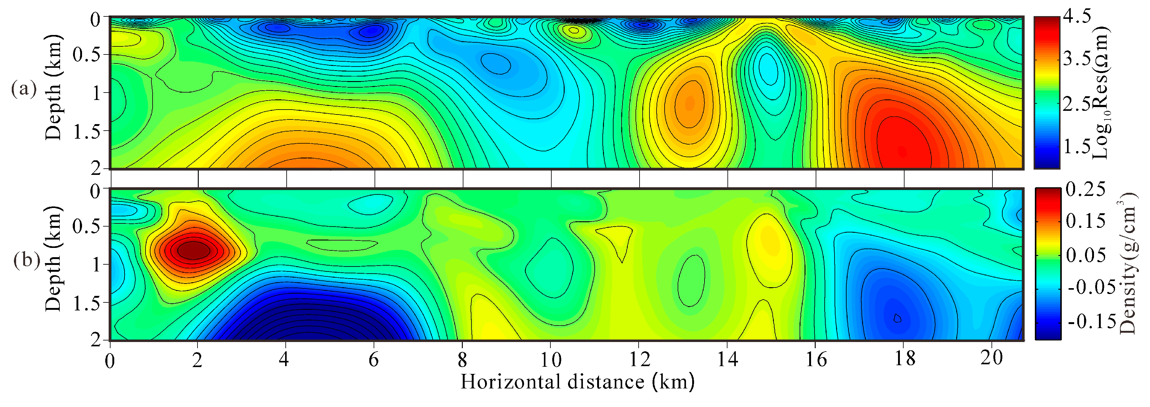
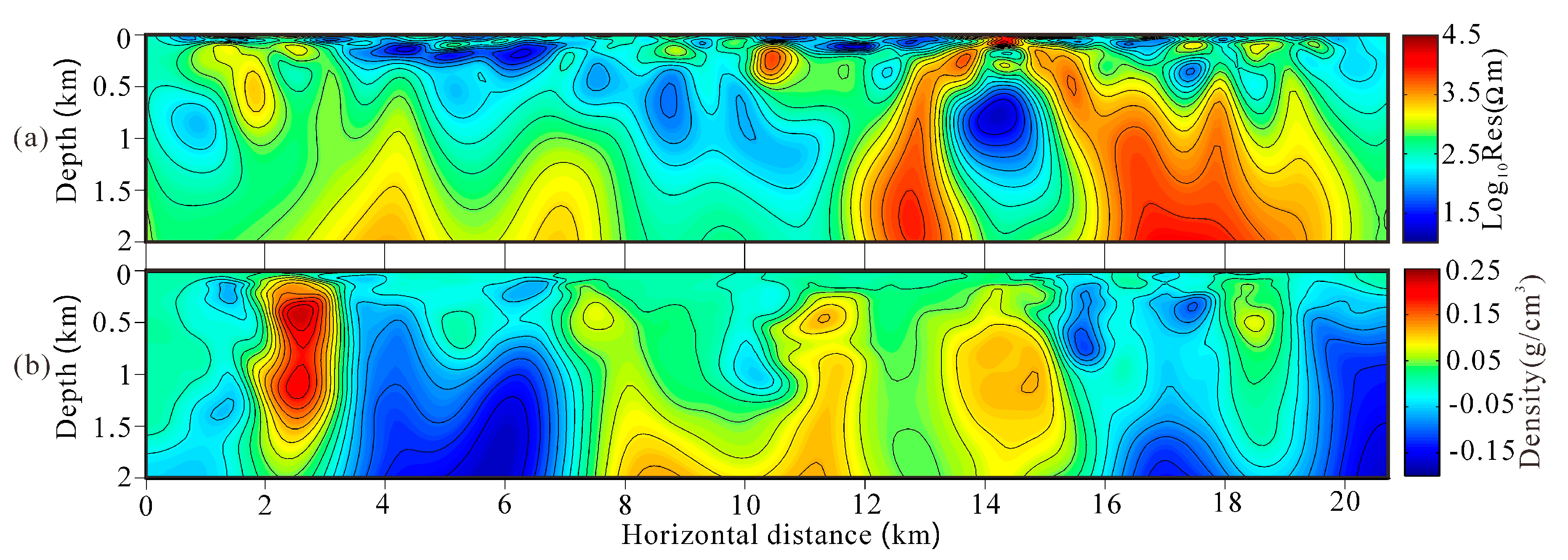
For the joint inversion experiment, the process started from the same homogeneous model as that of the separate inversion and the process converged consistently in terms of data fit until the misfits were reduced to values similar to those obtained for the corresponding separate inversion experiments. The RMS misfit values found after the smooth joint inversion were as follows: RMSCSAMT = 1.39 and RMSGRV = 0.55. Figure 14 shows the joint inversion results obtained by the smooth regularization method. We found a structural similarity between the density and resistivity models in the results of the smooth joint inversion, which was due to the contribution of the cross-gradient constraints in the objective function. However, the inversion results were relatively smooth, and a large area of divergence was exposed below the anomalous bodies. It was difficult to depict the sharp boundaries of the subsurface geological contact. The corresponding RMS misfit for each data set after the elastic-net joint inversion did not increase significantly and the values attained were: RMSCSAMT = 1.42 and RMSGRV = 0.24. Figure 15 shows the joint inversion results obtained by the elastic-net regularization method. We found that the elastic-net joint inversion method could generate much greater detail and a sharper boundary as well as better depth resolution. Compared with the smooth joint inversion results, the large area divergence phenomenon under the anomalous bodies was eliminated, and the fine anomalous bodies boundary appeared in the smooth region. The elastic-net joint inversion method provided more detailed information about the structure of the sources for further analysis than the separate inversion and smooth joint inversion methods.
5.4. Geological Interpretation of the Mining Area
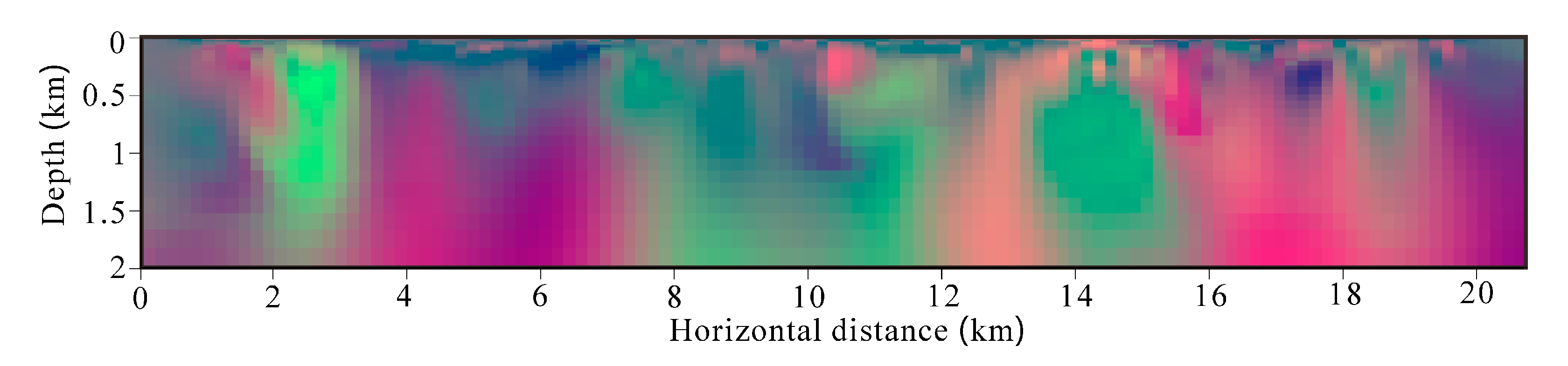
We conducted a geological interpretation of the higher resolution elastic-net joint inversion results. To facilitate geological interpretation, we combined the resistivity and residual density models obtained from the inversion into an RGB composite map of the (red–green–blue) mode. The RGB color space model is an additive color mixing model where red, green, and blue colors are superimposed on each other to achieve color mixing. The resistivity is represented in red, where a redder hue indicates the greater the resistivity; the residual density is in green, where a greener hue is a greater residual density; the blue was set to a value that had no change. The RGB composite map of the joint inversion model was generated by recombining the elastic-net joint inversion results (Figure 16). The composite image color contained the resistivity and residual density information, from which the inversion results could be analyzed intuitively to accurately identify, and possibly classify, the underground geological structures.
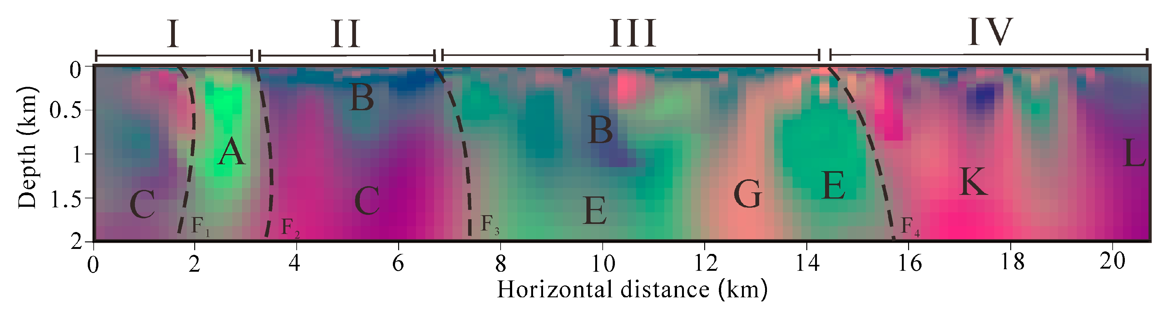
We carried out a geological interpretation for this area using the RGB composite image (Figure 16), the geological map (Figure 11), and a statistical table of stratigraphic lithology (Table 4). First, we divided the survey line into four segments (I–IV) according to the distribution of gravity anomalies. Segment I is located at the northern end of the study area and has the characteristics of a high-gravity anomaly. The surface reveals the Palaeozoic Majiagou formation and the Paleoproterozoic Zhenzumen formation, basalt is directly covered on the Paleoproterozoic, and it can be inferred that this was caused by the Paleoproterozoic basement uplift, as shown in unit A in Figure 17. Segment II appears as a low-gravity anomaly. Except for a large number of the Triassic Changbai formation and Tertiary Tumenzi formation, the others are covered by a large number of basalt of the Neogene Chuandishan formation. The resistivity of different depths of the Segment II showed obvious differences and could be roughly divided into two layers, unit B, which is a low resistive layer less than 1 km deep and unit C, a highly resistive layer greater than 1 km in depth. We concluded that unit B was caused by the volcanic subsidence basins of the Mesozoic and Cenozoic and unit C was caused by the intrusion of medium-acid volcanic rocks with low density and high resistivity. Combined with the Late Jurassic diorite exposed on the surface, it can be inferred that unit C is the intrusive Late Jurassic diorite (Figure 17). Segment III is a high-gravity anomaly zone. The surface of the Paleoproterozoic Dalizi formation, the Diaoyutai formation of the Qingbaikouan Period, and the Chaomidian and Gushan formations of the Late Cambrian are exposed. The rock density values of formation above-mentioned are relatively high, and the density of the overlying Mesozoic and Cenozoic caprocks are quite different. Therefore, the Paleozoic basin caused high gravity anomalies. The base of this segment is the Paleoproterozoic Dalizi formation (unit E), which is a favorable area for finding precious metals such as gold. Unit G has a high-resistance medium density characteristic, which is presumed to be the Diaoyutai formation quartz sandstone of the Qingbaikouan Period. Segment IV is located at the southern end of the study area and is a low-gravity anomaly area spread near the east and west. There are intrusive rocks such as Late Jurassic monzonitic granites and quartz monzodiorite on the surface. It was speculated that this segment was caused by the intrusion of volcanic rocks and medium-acid rocks with relatively low-density and high resistivity. Unit K is composed of Late Jurassic monzonitic granites and unit L is quartz monzodiorite. Moreover, through the geological map and the RGB composite map, we could infer the distribution of the fault structure (F1–F4) below the survey line. Based on the above inference results, we finally obtained a comprehensive interpretation profile, as shown in Figure 17. The corresponding lithostratigraphic units in Figure 17 are shown in Table 4.
At present, Segment I has been mined. The copper deposit is produced in the inter-layer fault zone of the Paleoproterozoic aging group. The ore-bearing horizon coincides with the intrusion space of the parent rock, that is, along the inter-laminar fault zone of the thick layer of dolomite in the Zhenzhumen formation. The output law of the ore body group is mainly based on the inner contact belt ore body, followed by the outer contact part. The cause of the Segment I deposit is due to the magma carrying mineral components and forming skarns along the contact zone at the edge of the rock mass, and the copper and sulfur being combined to precipitate and form the ore. The deposit belongs to the hydrothermal skarn type, and the skarn type ore is mainly composed of chalcopyrite, bornite, and molybdenite.
Compared to the above actual situation, we found that the comprehensive geological interpretation profile provided an accurate formation (Unit A) and fault structure position (F1–F2), which verified the accuracy of the proposed algorithm. According to the comprehensive interpretation profile results and the deposit formation of the known mining area, we have speculated on the ore-forming target area of other segments. It was preliminarily predicted that the ore-forming target area would be mainly concentrated near the fault structure (F3–F4). The interlaminar fault zone is the center of the regional tectonic, magmatic activity, and later ore-forming hydrothermal activities. Prospecting work should pay attention to the mineralization clues of the contact sites between the Mesozoic intrusive rocks and the Precambrian shallow metamorphic strata, particularly the Yanshanian intermediate-acid granites. Mineralization and alteration should also be given sufficient attention, and silicidation and muddy mixtures that are easily overlooked may also have mineralization indication significance. In this paper, the elastic-net joint inversion method could accurately divide the stratum structure and fault zone, and had the ability to find the prospecting target area, which provides a powerful basis for the mining of the deposit.
6. Conclusions
We presented a novel 2D joint inversion approach for imaging collocated magnetotelluric (MT) and gravity data with elastic-net regularization and cross-gradient constraints. We described the main features of the novel approach and first applied it to the synthetic model. Numerical modeling results indicated that the L2 norm penalty always performed the solution overly smooth and the L1 norm penalty always presented the solution too sparse. However, the elastic-net regularization method, a convex combination term of the L2 norm and L1 norm, could not only enforce the stability to preserve local smoothness, but could also enforce the sparsity to preserve sharp boundaries. Meanwhile, we found that the cross-gradient constraints could effectively complement the defects of different geophysical methods, improve the horizontal resolution of MT and the vertical resolution of gravity methods, and obtained a model with a remarkable structural resemblance. Moreover, this paper provided a field example in a regional exploration context of the elastic-net joint inversion of gravity and MT data. This illustrated that structurally reconciled models of a 20.7 km profile in the Linjiang copper mining area in Jilin Province, northeast China, fused into an RGB composite image, yielded a more detailed and meaningful integrated interpretation of the subsurface. This case history highlights the advantages of using structurally reconciled models for integrated geophysical interpretations and showcases the power of RGB imaging in facilitating interpretation. Elastic-net joint inversion leads to more detailed and sharp boundary models that depict more property zones and may leads to the less ambiguous distinction of geologic materials. The RGB composite image adequately characterized the stratigraphic sequences and fault structure, and showed compatibility with the underground distribution structure of the identified deposits. This provides a favorable basis for unexplored areas, both in the formation sequence and fault location.
Whereas the proposed method proved its suitability for improved and integrated geophysical interpretation, it also illustrated that an improved resolution was largely driven by the accuracy of the individual geophysical modeling strategies and geophysical data. It is evident that strategies such as the incorporation of magnetic data, high precision seismic reflection data, or cross-hole data should lead to a higher resolution in imaging. Furthermore, these particular strategies can be adopted within the elastic-net joint inversion scheme.
Author Contributions
Conceptualization, R.Z.; methodology, R.Z., T.L.; software, R.Z.; validation, T.L.; formal analysis, R.Z., T.L.; investigation, R.Z., T.L.; resources, R.Z., T.L.; data curation, R.Z., T.L.; writing—original draft preparation, R.Z.; writing—review and editing, R.Z., T.L., S.Z., X.D.; supervision, T.L.; project administration, T.L.; funding acquisition, T.L., S.Z.
Funding
This research was funded by the Nation Key R&D program of China (2017YFC0601606), Jilin University PhD Graduate Interdisciplinary Research Funding Project (10183201838), the National Postdoctoral Program for Innovative Talents (B 2017-014), and China Postdoctoral Science Foundation funded project (2018M630323).
Conflicts of Interest
The authors declare no conflict of interest.
References
- Engl, H.W.; Ramlau, R. Regularization of Inverse Problems; Springer: Berlin, Germany, 2015. [Google Scholar]
- Honerkamp, J.; Weese, J. Tikhonovs regularization method for ill-posed problems. A comparison of different methods for the determination of the regularization parameter. Contin. Mech. Thermodyn. 1990, 2, 17–30. [Google Scholar] [CrossRef]
- Tikhonov, A.N.; Dsh, B.; Griogolava, I.V. Interaction of ubisemiquinone with the high-potential iron-sulfur center of submitochondrial particle succinate dehydrogenase. EPR study at 240 and 12 degrees K. Biofizika 1977, 22, 734. [Google Scholar] [PubMed]
- Li, Y.G.; Oldenburg, D.W. 3D inversion of magnetic data. Geophysics 1996, 61, 394–408. [Google Scholar] [CrossRef]
- Li, Y.G.; Oldenburg, D.W. Fast inversion of large-scale magnetic data using wavelet transforms and a logarithmic barrier method. Geophys. J. Int. 2003, 152, 251–265. [Google Scholar] [CrossRef] [Green Version]
- Pilkington, M. 3D magnetic imaging using conjugate gradients. Geophysics 1997, 62, 1132–1142. [Google Scholar] [CrossRef]
- Cella, F.; Fedi, M. Inversion of potential field data using the structural index as weighting function rate decay. Geophys. Prospect. 2012, 60, 313–336. [Google Scholar] [CrossRef]
- Paoletti, V.; Ialongo, S.; Florio, G.; Fedi, M.; Cella, F. Self-constrained inversion of potential fields. Geophys. J. Int. 2013, 195, 854–869. [Google Scholar] [CrossRef] [Green Version]
- Chopra, A.; Lian, H. Total variation, adaptive total variation and nonconvex smoothly clipped absolute deviation penalty for denoising blocky images. Pattern Recognit. 2010, 43, 2609–2619. [Google Scholar] [CrossRef] [Green Version]
- Figueiredo, M.A.T.; Dias, J.B.; Oliveira, J.P.; Nowak, R.D. On total variation denoising: A new majorization-minimization algorithm and an experimental comparison with wavalet denoising. In Proceedings of the IEEE International Conference on Image Processing (ICIP 2006), Atlanta, GA, USA, 8–11 October 2006; pp. 2633–2636. [Google Scholar]
- Li, Q.; Micchelli, C.A.; Shen, L. A proximity algorithm accelerated by Gauss-Seidel iterations for L1/TV denoising models. Inverse Probl. 2012, 28, 095003. [Google Scholar] [CrossRef]
- Guitton, A. Blocky regularization schemes for full waveform inversion. Geophys. Prospect. 2012, 60, 870–884. [Google Scholar] [CrossRef]
- Strong, D.; Chan, T. Edge-preserving and scale-dependent properties of total variation regularization. Inverse Probl. 2003, 19, 165–187. [Google Scholar] [CrossRef]
- Daubechies, I.; DeVore, R.; Fornasier, M. Iteratively reweighted least squares minimization for sparse recovery. Commun. Pure Appl. Math. 2010, 63, 1–38. [Google Scholar] [CrossRef]
- Donoho, D.L. Compressed sensing. IEEE Trans. Inf. Theory 2006, 52, 1289–1306. [Google Scholar] [CrossRef]
- Jin, B.T.; Maass, P. Sparsity Regularization for Parameter Identification Problems. Inverse Probl. 2012, 28, 123001. [Google Scholar] [CrossRef]
- Loris, I.; Nolet, G.; Daubechies, I.; Dahlen, F.A. Tomographic inversion using ℓ1-norm regularization of wavelet coefficients. Geophys. J. Int. 2007, 170, 359–370. [Google Scholar] [CrossRef]
- Wang, Y.; Yang, C.; Cao, J. On Tikhonov regularization and compressive sensing for seismic signal processing. Math. Models Meth. Appl. Sci. 2012, 22, 1150008. [Google Scholar] [CrossRef]
- Farquharson, C.G.; Oldenburg, D.W.; Routh, P.S. Simultaneous 1D inversion of loop-loop electromagnetic data for magnetic susceptibility and electrical conductivity. Geophysics 2003, 68, 1857–1869. [Google Scholar] [CrossRef]
- Farquharson, C.G. Constructing piecewise-constant models in multidimensional minimum-structure inversions. Geophysics 2008, 73, K1–K9. [Google Scholar] [CrossRef]
- Loke, M.H.; Acworth, I.; Dahlin, T. A comparison of smooth and blocky inversion methods in 2D electrical imaging surveys. Explor. Geophys. 2003, 34, 182–187. [Google Scholar] [CrossRef]
- Van Zon, T.; Roy-Chowdhury, K. Structural inversion of gravity data using linear programming. Geophysics 2006, 71, J41–J50. [Google Scholar] [CrossRef]
- Anbari, M.E.; Mkhadri, A. Penalized regression combining the L1 norm and a correlation based penalty. Sankhya B 2014, 76, 82–102. [Google Scholar] [CrossRef]
- Zou, H.; Hastie, T. Regularization and variable selection via the elastic net. J. R. Stat. Soc. Ser. B Stat. Methodol. 2005, 67, 301–320. [Google Scholar] [CrossRef] [Green Version]
- Jin, B.; Lorenz, D.; Schiffler, S. Elastic-net regularization: error estimates and active set methods. Inverse Probl. 2009, 25, 1595–1610. [Google Scholar] [CrossRef]
- Mol, C.D.; Vito, E.D.; Rosasco, L. Elastic-net regularization in learning theory. J. Complex. 2009, 25, 201–230. [Google Scholar] [CrossRef] [Green Version]
- Wang, J.; Han, B.; Wang, W. Elastic-net regularization for nonlinear electrical impedance tomography with a splitting approach. Appl. Anal. 2018, 2017, 1–17. [Google Scholar] [CrossRef]
- Zhdanov, M.S.; Alfouzan, F.A.; Cox, L.; Alotaibi, A.; Alyousif, M.; Sunwall, D.; Endo, M. Large-Scale 3D Modeling and Inversion of Multiphysics Airborne Geophysical Data: A Case Study from the Arabian Shield, Saudi Arabia. Minerals 2018, 8, 271. [Google Scholar] [CrossRef]
- Tillmann, A.; Stöcker, T. A new approach for the joint inversion of seismic and geoelectric data. In Proceedings of the 63rd EAGE Conference and Technical Exhibition, Amsterdam, The Netherlands, 11–15 June 2000. [Google Scholar]
- Jones, A.G.; Fishwick, S.; Evans, R.L.; Spratt, J.E. Correlation of lithospheric velocity and electrical conductivity for Southern Africa. 2009. Available online: https://www.researchgate.net/publication/252588025_Correlation_of_lithospheric_velocity_and_electrical_conductivity_for_Southern_Africa (accessed on 2 July 2019).
- Hoversten, G.M.; Cassassuce, F.; Gasperikova, E.; Newman, G.A.; Chen, J.; Rubin, Y.; Hou, Z.; Vasco, D. Direct reservoir parameter estimation using joint inversion of marine seismic AVA and CSEM data. Geophysics 2006, 71, C1–C13. [Google Scholar] [CrossRef] [Green Version]
- Harris, P.; MacGregor, L. Determination of reservoir properties from the integration of CSEM, seismic, and well-log data. First Break 2006, 25, 53–59. [Google Scholar]
- Gallardo, L.A.; Meju, M.A. Characterization of heterogeneous near-surface materials by joint 2D inversion of dc resistivity and seismic data. Geophys. Res. Lett. 2003, 30, 1658. [Google Scholar] [CrossRef]
- Gallardo, L.A.; Meju, M.A. Joint two-dimensional DC resistivity and seismic traveltime inversion with crossgradients constraints. J. Geophys. Res. Solid Earth 2004, 109, 3311–3315. [Google Scholar] [CrossRef]
- Colombo, D.; De Stefano, M. Geophysical modeling via simultaneous joint inversion of seismic, gravity, and electromagnetic data: Application to prestack depth imaging. Lead. Edge 2007, 26, 326–331. [Google Scholar] [CrossRef]
- Hamdan, H.A.; Vafidis, A. Joint inversion of 2D resistivity and seismic travel time data to image saltwater intrusion over karstic areas. Environ. Earth Sci. 2013, 68, 1877–1885. [Google Scholar] [CrossRef]
- Bennington, N.L.; Zhang, H.; Thurber, C.H. Joint inversion of seismic and magnetotelluric data in the park field region of california using the normalized cross-gradient constraint pure and applied. Geophysics 2015, 172, 1033–1052. [Google Scholar]
- Li, T.L.; Zhang, R.Z.; Pak, Y.C. Joint Inversion of magnetotelluric and first-arrival wave seismic traveltime with cross-gradient constraints. J. Jilin Univ. Earth Sci. Ed. 2015, 45, 952–961. [Google Scholar]
- Li, T.L.; Zhang, R.Z.; Pak, Y.C. Multiple joint inversion of geophysical data with sub-region cross-gradient constraints. Chin. J. Geophys. 2016, 59, 2979–2988. [Google Scholar]
- Zhang, R.Z.; Li, T.L.; Deng, H. 2D joint inversion of MT, gravity, magnetic and seismic first-arrival traveltime with cross-gradient constraints. Chin. J. Geophys. 2019, 62, 2139–2149. [Google Scholar]
- Moorkamp, M.; Heincke, B.; Jegen, M.; Roberts, A.W.; Hobbs, R.W. A framework for 3D joint inversion of MT, gravity and seismic refraction data. Geophys. J. Int. 2011, 184, 477–493. [Google Scholar] [CrossRef]
- Gallardo, L.A.; Fontes, S.L.; Meju, M.A.; Buonora, M.P.; de Lugao, P.P. Robust geophysical integration through structure-coupled joint inversion and multispectral fusion of seismic reflection, magnetotelluric, magnetic, and gravity images: Example from Santos Basin, offshore Brazil. Geophysics 2012, 77, B237–B251. [Google Scholar] [CrossRef]
- Linde, N.; Binley, A.; Tryggvason, A.; Pedersen, L.B.; Revil, A. Improved hydrogeophysical characterization using joint inversion of cross-hole electrical resistance and ground-penetrating radar travel-time data. Water Resour. Res. 2006, 42, W12404. [Google Scholar] [CrossRef]
- Linde, N.; Tryggvason, A.; Peterson, J.E.; Hubbard, S.S. Joint inversion of crosshole radar and seismic traveltimes acquired at the South Oyster Bacterial Transport Site. Geophysics 2008, 73, G29–G37. [Google Scholar] [CrossRef] [Green Version]
- Zhdanov, M.S.; Gribenko, A.; Wilson, G. Generalized joint inversion of multimodal geophysical data using Gramian constraints. Geophys. Res. Lett. 2012, 39, L09301. [Google Scholar] [CrossRef]
- Haber, E.; Holtzman Gazit, M. Model Fusion and Joint Inversion. Surv. Geophys. 2013, 34, 675–695. [Google Scholar] [CrossRef]
- deGroot-Hedlin, C.D.; Constable, S.C. Occam’s inversion to generate smooth, two-dimensional models from magnetotelluric data. Geophysics 1990, 55, 1613–1624. [Google Scholar] [CrossRef]
- Wannamaker, P.E.; Stodt, J.A.; Rijo, L. A stable finite element solution for two-dimensional magnetotelluric modeling. Geophys. J. Int. 1987, 88, 277–296. [Google Scholar] [CrossRef]
- Singh, B. Simultaneous computation of gravity and magnetic anomalies resulting from a 2D object. Geophysics 2002, 67, 801–806. [Google Scholar] [CrossRef]
- Tarantola, A. Inversion problem theory: Methods for data fitting and model parameter estimation. Phys. Earth Planet. Inter. 1987, 57, 350–351. [Google Scholar]
- Byrd, R.H.; Payne, D.A. Convergence of the Iteratively Re-Weighted Least Squares Algorithm for Robust Regression; Johns Hopkins University: Baltimore, MD, USA, 1979. [Google Scholar]
- Wolke, R.; Schwetlick, H. Iteratively reweighted least squares: Algorithms, convergence analysis, and numerical comparisons. SIAM J. Sci. Comput. 1988, 9, 907–921. [Google Scholar] [CrossRef]
- Chartrand, R.; Yin, W. Iteratively reweighted algorithms for compressive sensing. In Proceedings of the 33rd International Conference on Acoustics, Speech, and Signal Processing, Las Vegas, NV, USA, 28 March–4 April 2008; pp. 3869–3872. [Google Scholar]
- Last, B.J.; Kubik, K. Compact gravity inversion. Geophysics 1983, 48, 713–721. [Google Scholar] [CrossRef]
- Zhdanov, M.S. Geophysical Inverse Theory and Regularization Problems; Elsevier: Amsterdam, The Netherlands, 2002. [Google Scholar]
- Rudin, L.; Osher, S.; Fatemi, E. Nonlinear total variation based noise removal algorithms. Phys. D 1992, 60, 259–268. [Google Scholar] [CrossRef]
Figure 1.
MT separate inversion results obtained using different regularization methods. (a) Resistivity true model; (b) Resistivity inversion model using L2 regularization; (c) Resistivity inversion model using L1 regularization; (d) Resistivity inversion model using elastic-net regularization; (e) Resistivity inversion model using TV regularization; (f) Resistivity inversion model using focusing regularization. The black box indicates the boundary of the anomalous body.

Figure 2.
Gravity separate inversion results obtained using different regularization methods. (a) Density true model; (b) Density inversion model using L2 regularization; (c) Density inversion model using L1 regularization; (d) Density inversion model using elastic-net regularization; (e) Density inversion model using TV regularization; (f) Density inversion model using focusing regularization. The black box indicates the boundary of the anomalous body.

Figure 3.
RMS misfit evolution of the MT separate inversion (a) and gravity separate inversion (b).

Figure 4.
The MT inversion results obtained using separate and joint inversion. (a) Resistivity true model; (b) Resistivity separate inversion model using L2 regularization; (c) Resistivity separate inversion model using elastic-net regularization; (d) Resistivity joint inversion model using L2 regularization; (e) Resistivity joint inversion model using elastic-net regularization. The black box indicates the boundary of the anomalous body.

Figure 5.
The gravity inversion results obtained using separate and joint inversion. (a) Density true model; (b) Density separate inversion model using L2 regularization; (c) Density separate inversion model using elastic-net regularization; (d) Density joint inversion model using L2 regularization; (e) Density joint inversion model using elastic-net regularization. The black box indicates the boundary of the anomalous body.

Figure 6.
The RMS misfit evolution of the MT inversion (a) and gravity inversion (b).

Figure 7.
The true model of MT and gravity methods. Model 1 (a,b); Model 2 (c,d); Model 3 (e,f); Resistivity models (a,c,e) ; Density models (b,d,f).
Figure 7.
The true model of MT and gravity methods. Model 1 (a,b); Model 2 (c,d); Model 3 (e,f); Resistivity models (a,c,e) ; Density models (b,d,f).

Figure 8.
The model response results for three models of resistivity and density. The theoretical model responses of resistivity models obtained by TM mode (a1–a3); The theoretical model responses of density models (e1–e3); The resistivity model responses with 5% noise obtained by TM mode (b1–b3); The density model responses with 5% noise (f1–f3); The resistivity model responses with 10% noise obtained by TM mode (c1–c3); The density model responses with 5% noise. (g1–g3); The resistivity model responses with 20% noise obtained by TM mode (d1–d3); The density model responses with 20% noise (h1–h3).

Figure 9.
The MT and gravity inversion results obtained using elastic-net joint inversion. Resistivity true model (a1–a3); Density true model (e1–e3); The MT inversion results with 5% noise (b1–b3); The gravity inversion results with 5% noise (f1–f3); The MT inversion results with 10% noise (c1–c3); The gravity inversion results with 10% noise (g1–g3); The MT inversion results with 20% noise (d1–d3); The gravity inversion results with 20% noise (h1–h3).

Figure 10.
Location (red rectangle) and tectonic background map of the study area.

Figure 11.
The geological map of the Linjiang copper mining area.

Figure 12.
Observation data of the survey line: apparent resistivity in TM mode (a) and residual anomaly (b).
Figure 12.
Observation data of the survey line: apparent resistivity in TM mode (a) and residual anomaly (b).

Figure 13.
The results of separate inversion: resistivity model (a), residual density model (b).

Figure 14.
The results of joint inversion using smooth regularization: resistivity model (a), residual density model (b).
Figure 14.
The results of joint inversion using smooth regularization: resistivity model (a), residual density model (b).

Figure 15.
The results of joint inversion using elastic-net regularization: resistivity model (a), residual density model (b).
Figure 15.
The results of joint inversion using elastic-net regularization: resistivity model (a), residual density model (b).

Figure 16.
The RGB composite image of the elastic-net joint inversion.

Figure 17.
Comprehensive geological interpretation profile.


Table 1.
The resistivities and residual densities of synthetic model 1.
| Unit | Resistivity Model | Residual Density Model |
|---|---|---|
| A | 1000 Ω·m | −1000 kg/m3 |
| B | 10 Ω·m | 1000 kg/m3 |
| C | 100 Ω·m | 0 kg/m3 |
Table 2.
The resistivities and residual densities of synthetic model 2.
| Unit | Resistivity Model | Residual Density Model |
|---|---|---|
| A | 1000 Ω·m | 700 kg/m3 |
| B | 10 Ω·m | 1000 kg/m3 |
| C | 100 Ω·m | 0 kg/m3 |
Table 3.
The resistivities and residual densities of the synthetic model.
| Unit | Resistivity Model | Residual Density Model | Size | |
|---|---|---|---|---|
| A | 10 Ω·m | 1000 kg/m3 | 1 × 1 km2 | Model 1 |
| B | 10 Ω·m | 1000 kg/m3 | 1 × 1 km2 | |
| C | 100 Ω·m | 0 kg/m3 | - | |
| A | 10 Ω·m | 1000 kg/m3 | 0.5 × 0.5 km2 | Model 2 |
| B | 10 Ω·m | 1000 kg/m3 | 0.5 × 0.5 km2 | |
| C | 100 Ω·m | 0 kg/m3 | - | |
| A | 10 Ω·m | 1000 kg/m3 | 0.2 × 0.2 km2 | Model 3 |
| B | 10 Ω·m | 1000 kg/m3 | 0.2 × 0.2 km2 | |
| C | 100 Ω·m | 0 kg/m3 | - |
Table 4.
Statistical table of stratigraphic lithology.
| Geological Time | Lithostratigraphic Units | Lithology | Density | Resistivity | Unit | |
|---|---|---|---|---|---|---|
| Era | Period | Formation | Average (g/cm3) | Average (Ω·m) | ||
| Cenozoic | Neogene | Junjianshan (N2j) | Basalt | 2.55 | 500 | B |
| Chuandishan (N1c) | Basalt | 2.55 | 506 | B | ||
| Tumenzi (N1t) | Basalt | 2.57 | 404 | B | ||
| Mesozoic | Triassic | Changbai (T3c) | Tuff | 2.6 | 274 | B |
| Paleozoic | Ordovician | Majiagou (Q2m) | Limestone | 2.75 | 3386 | |
| Liangjiashan (Q1l) | Micrite | 2.65 | 524 | |||
| Cambrian | Caomidian (Є3c) | Limestone | 2.70 | 2975 | ||
| Gushan (Є3g) | Schist | 2.69 | 2666 | |||
| Proterozoic | Sinian | Wanlong (Z1w) | Limestone | 2.72 | 6244 | |
| Qingbaikouan | Diaoyutai (Nhd) | Feldspathic quartz sandstone | 2.62 | 3227 | G | |
| Paleoproterozoic | Dalizi (Pt1dl) | Eryun schist with marble | 2.75 | 1140 | E | |
| Huashan (Pt1h) | Cloud schist | 2.80 | 1957 | A | ||
| Zhenzhumen (Pt1z) | Dolomitic marble | 2.78 | 2615 | A | ||
© 2019 by the authors. Licensee MDPI, Basel, Switzerland. This article is an open access article distributed under the terms and conditions of the Creative Commons Attribution (CC BY) license (http://creativecommons.org/licenses/by/4.0/).
Share and Cite
MDPI and ACS Style
Zhang, R.; Li, T.; Zhou, S.; Deng, X. Joint MT and Gravity Inversion Using Structural Constraints: A Case Study from the Linjiang Copper Mining Area, Jilin, China. Minerals 2019, 9, 407. https://doi.org/10.3390/min9070407
AMA Style
Zhang R, Li T, Zhou S, Deng X. Joint MT and Gravity Inversion Using Structural Constraints: A Case Study from the Linjiang Copper Mining Area, Jilin, China. Minerals. 2019; 9(7):407. https://doi.org/10.3390/min9070407
Chicago/Turabian StyleZhang, Rongzhe, Tonglin Li, Shuai Zhou, and Xinhui Deng. 2019. "Joint MT and Gravity Inversion Using Structural Constraints: A Case Study from the Linjiang Copper Mining Area, Jilin, China" Minerals 9, no. 7: 407. https://doi.org/10.3390/min9070407
Note that from the first issue of 2016, this journal uses article numbers instead of page numbers. See further details here.