
Spatial Component Analysis to Improve Mineral Estimation Using Sentinel-2 Band Ratio: Application to a Greek Bauxite Residue

 , , and
Abstract
:1. Introduction
1.1. Recovery of Minerals from Stockpiles and Tailings
1.2. Exploitation of Remote Sensing Information
2. Materials and Methods
2.1. Co-Regionalization Model and Application: Current Practice
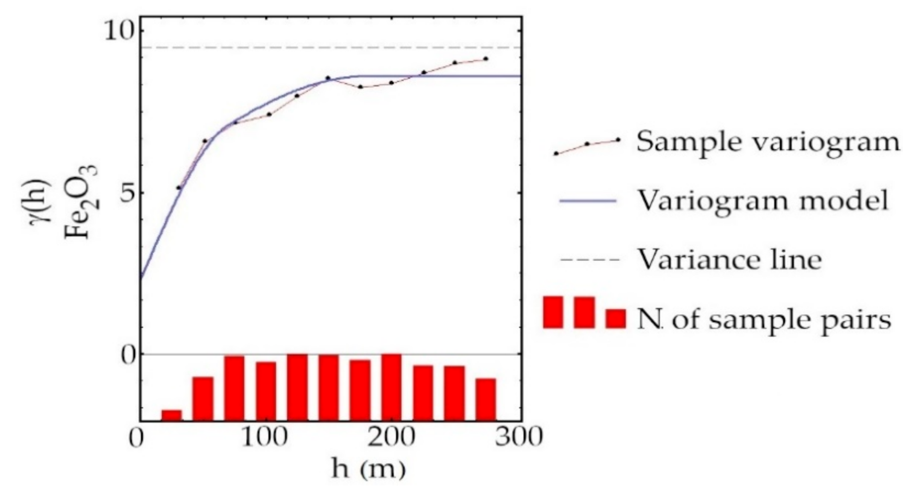
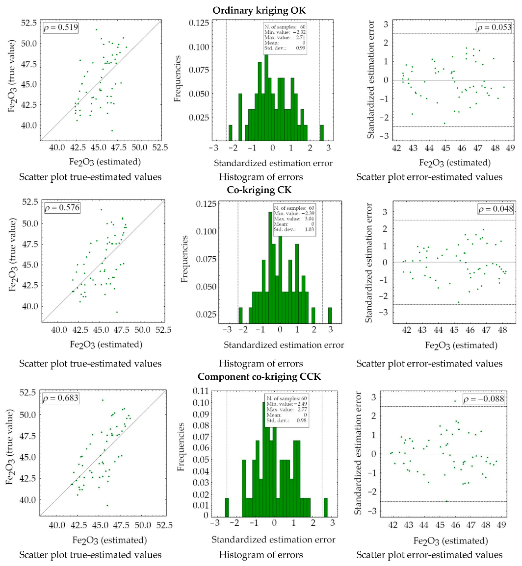
- Using one variable: iron samples, spatial variability analysis of target variable (sample variogram and its model), and finally using the OK estimation method;
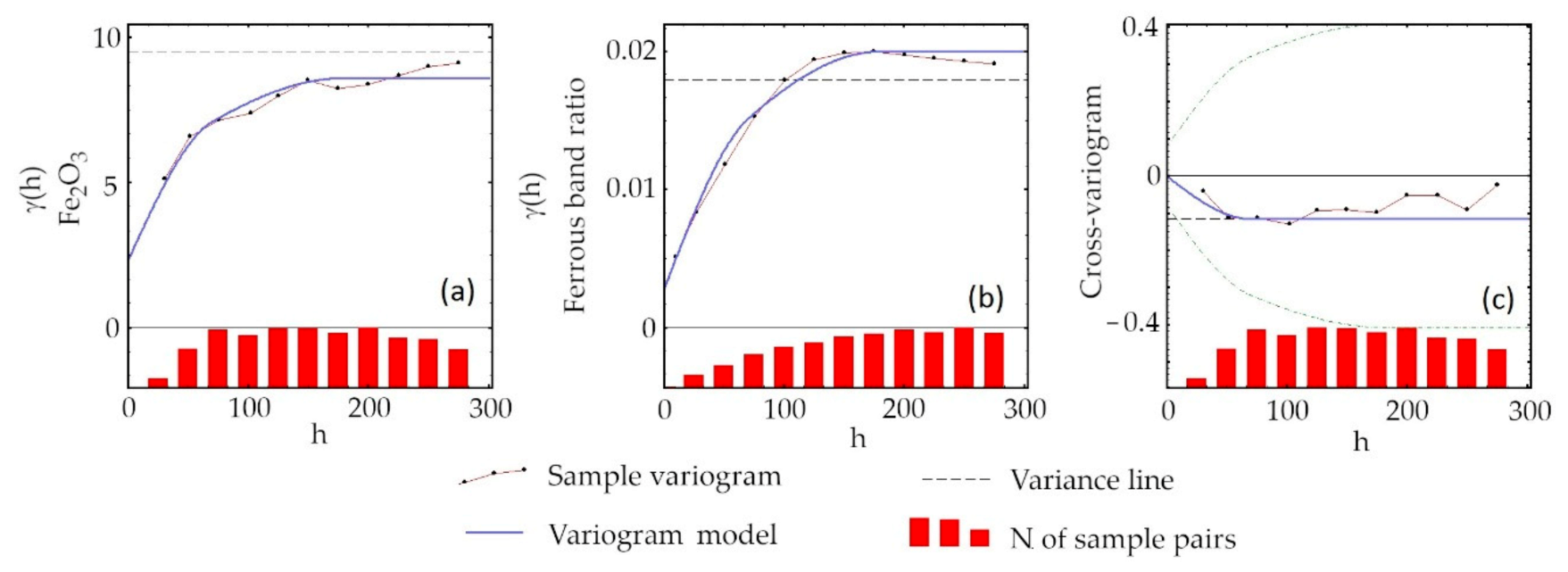
- Adding extra information (as an example band ratio of iron as the secondary variable): spatial variability analysis of target variable (sample variogram and its model) and the secondary variable, the cross-correlation analysis between the target variable and the secondary variable, and finally using the CK estimation method.
- At the end, to compare the map accuracies results, cross-validation should be performed to check if adding information can improve the results.
- The cross-validation;
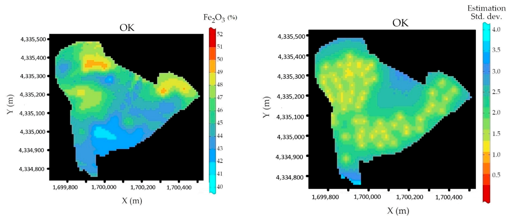
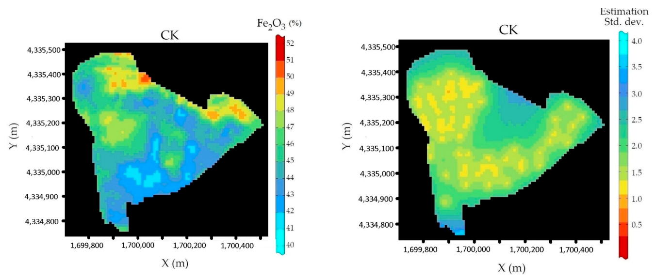
- The estimation maps of minerals;
- The maps of estimation variance.
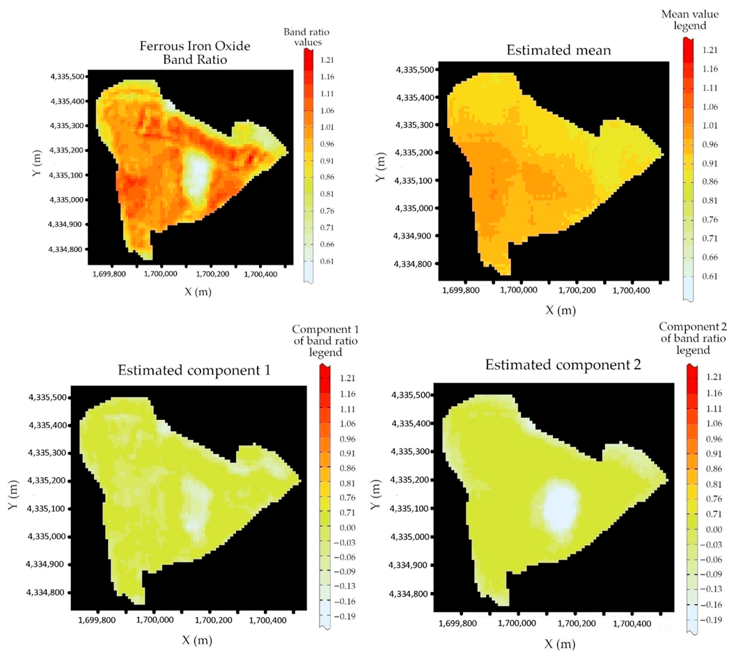
2.2. New Perspective: Use of Spatial Components
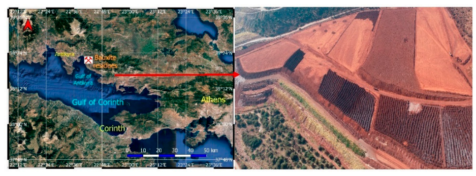
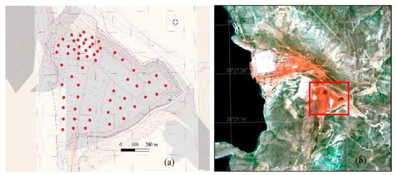
2.3. Case Study: The Bauxite Residuals of Greece
3. Results
4. Discussion
5. Conclusions
- Remote sensing data are essential when mapping a surface feature, such as mapping the iron concentration variability;
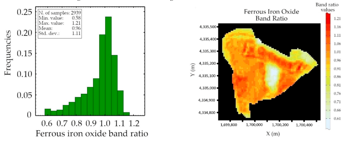
- Band ratio can be considered an important auxiliary variable in geostatistical modeling, when there is correlation between in field samples and band ratios;
- Component co-kriging is an efficient method and, in case of high correlation coefficient between one component of the auxiliary variable and the main variable (in this work, the iron concentration), it can substantially improve the mapping results.
Author Contributions
Funding
Data Availability Statement
Acknowledgments
Conflicts of Interest
References
- World Economic Forum (2005) Mining & Metals in a Sustainable World 2050, Ind Agenda. Available online: https://www.weforum.org/press/2015/09/mining-and-metals-in-a-sustainable-world-2050-report-launch/ (accessed on 20 May 2021).
- UN General Assembly (2015) Transforming Our World: The 2030 Agenda for Sustainable Development 21 October 2015. A/RES/70/1. Available online: https://www.refworld.org/docid/57b6e3e44.html (accessed on 20 May 2021).
- Lebre, E.; Corder, G.D.; Golev, A. The role of the mining industry in a circular economy—A framework for resource management at the mine site level. J. Ind. Ecol. 2017, 21, 662–672. [Google Scholar] [CrossRef]
- Mancini, L.; Sala, S. Social impact assessment in the mining sector: Review and comparison of indicators frameworks. Resour. Policy 2018, 57, 98–111. [Google Scholar] [CrossRef]
- COM (2020) 474 Final Communication from the Commission to the European Parliament, the Council, the European Economic and Social Committee and the Committee of the Regions Critical Raw Materials Resilience: Charting a Path towards Greater Security and Sustainability. Available online: https://eur-lex.europa.eu/legal-content/EN/TXT/?uri=CELEX%3A52020DC0474 (accessed on 20 May 2021).
- Ferro, P.; Bonollo, F. Materials selection in a critical raw materials perspective. Mater. Des. 2019, 177, 107848. [Google Scholar] [CrossRef]
- Jutz, S.; Milagro-Perez, M. Copernicus Program. Compr. Remote Sens. 2017, 1, 150–191. [Google Scholar] [CrossRef]
- Follador, M. Using remote sensing for mineral characterization in tropical forest areas of Brazil, GIS and Spatial Analysis. In 2005 Annual Conference of the International Association for Mathematical Geology; IAMG: Fortaleza, Brazil, 2005; pp. 127–132. ISBN 0973422017. [Google Scholar]
- Ferrier, G. Application of imaging spectrometer data in identifying environmental pollution caused by mining at Rodaquilar, Spain. Remote Sens. Environ. 1999, 68, 125–137. [Google Scholar] [CrossRef]
- Mars, J.C.; Crowley, J.K. Mapping mine wastes and analyzing areas affected by selenium-rich water runoff in southeast Idaho using AVIRIS imagery and digital elevation data. Remote Sens. Environ. 2003, 84, 422–436. [Google Scholar] [CrossRef]
- Choe, E.; Van der Meer, F.; Van Ruitenbeek, F.; Van der Werff, H.; Boudewijn de Smeth, B.; Kim, K.W. Mapping of heavy metal pollution in stream sediments using combined geochemistry, field spectroscopy, and hyperspectral remote sensing: A case study of the Rodalquilar mining area, SE Spain. Remote Sens. Environ. 2008, 112, 3222–3233. [Google Scholar] [CrossRef]
- Pascucci, S.; Belviso, C.; Cavalli, R.M.; Palombo, A.; Pignatti, S.; Santini, F. Using imaging spectroscopy to map red mud dust waste: The Podgorica aluminum complex case study. Remote Sens. Environ. 2012, 123, 139–154. [Google Scholar] [CrossRef]
- Werner, T.T.; Bebbington, A.; Gregory, G. Assessing impacts of mining: Recent contributions from GIS and remote sensing. Extr. Ind. Soc. 2019, 6, 993–1012. [Google Scholar] [CrossRef]
- Lopez-Granados, F.; Jurado-Exposito, M.; Pena-Barragan, J.M.; Garcia-Torres, L. Using geostatistical and remote sensing approaches for mapping soil properties. Eur. J. Agron. 2005. [Google Scholar] [CrossRef]
- Liu, Y.; Cao, G.; Zhao, N.; Mulligan, K.; Ye, X. Improve ground-level PM2.5 concentration mapping using a random forests-based geostatistical approach. Environ. Pollut. 2018. [Google Scholar] [CrossRef]
- Bzdęga, K.; Zarychta, A.; Urbisz, A.; Szporak-Wasilewska, S.; Ludynia, M.; Fojcik, B.; Tokarska-Guzik, B. Geostatistical models with the use of hyperspectral data and seasonal variation—A new approach for evaluating the risk posed by invasive plants. Ecol. Indic. 2021. [Google Scholar] [CrossRef]
- Matheron, G. The intrinsic random functions and their applications. Adv. Appl. Probab. 1973, 5, 439–468. [Google Scholar] [CrossRef] [Green Version]
- Wackernagel, H. Multivariate Geostatistics. In An Introduction with Applications; Springer: Heidelberg/Berlin, Germany, 2003; pp. 121–208. [Google Scholar] [CrossRef]
- Chiles, J.P.; Delfiner, P. Geostatistics Modeling Spatial Uncertainty, 2th ed.; Wiley: Hoboken, NJ, USA, 2012; pp. 118–177. ISBN 978-0-470-18315-1. [Google Scholar]
- Van der Meer, F. Extraction of mineral absorption features from high-spectral resolution data using non-parametric geostatistical techniques. Int. J. Remote Sens. 1994, 15, 2193–2214. [Google Scholar] [CrossRef]
- Yamaguchi, Y.; Kahle, A.B.; Tsu, H.; Kawakami, T.; Pniel, M. Overview of Advanced Spaceborne Thermal Emission and Reflection Radiometer (ASTER). IEEE Trans. Geosci. Remote Sens. 1998, 36, 1062–1071. [Google Scholar] [CrossRef] [Green Version]
- Yamaguchi, Y.; Fujisada, H.; Tsu, H.; Sato, I.; Watanabe, H.; Kato, M.; Kudoh, M.; Kahle, A.B.; Pniel, M. ASTER early image evaluation. Adv. Space Res. 2001, 28, 69–76. [Google Scholar] [CrossRef]
- Rouskov, K.; Popov, K.; Stanislav Stoykov, S.; Yamaguchi, Y. Some applications of the remote sensing in geology by using of ASTER images. In Proceedings of the Scientific Conference “SPACE ECOLOGY SAFETY” with International Participation, Sofia, Bulgaria, 10–13 June 2005. [Google Scholar]
- de Morais, M.C.; Martins Junior, P.P.; Paradella, W.R. Multi-scale approach using remote sensing images to characterize the iron deposit N1 influence areas in Carajás Mineral Province (Brazilian Amazon). Environ. Earth Sci. 2012, 66, 2085–2096. [Google Scholar] [CrossRef]
- Van der Meer, F.D.; Van der Werff, H.M.A.; Van Ruitenbeek, F.J.A.; Hecker, C.A.; Bakker, W.H.; Noomen, M.F.; Van der Meijde, M.; Carranza, E.J.M.; de Smeth, J.B.; Woldai, T. Multi- and hyperspectral geologic remote sensing: A review. Int. J. Appl. Earth Obs. 2012, 14, 112–128. [Google Scholar] [CrossRef]
- Gopinathan, P.; Parthiban, S.; Magendran, T.; Al-Quraishi, A.M.; Singh, A.K.; Singh, P.K. Mapping of ferric (Fe3+) and ferrous (Fe2+) iron oxides distribution using band ratio techniques with ASTER data and geochemistry of Kanjamalai and Godumalai, Tamil Nadu, south India. Remote Sens. Appl. Soc. Environ. 2020, 18, 100306. [Google Scholar] [CrossRef]
- Guha, A.; Singh, V.K.; Parveen, R.; Vinod Kumar, K.; Jeyaseelan, A.T.; Dhanamjaya Rao, E.N. Analysis of ASTER data for mapping bauxite rich pockets within high altitude lateritic bauxite, Jharkhand, India. Int. J. Appl. Earth Obs. Geoinf. 2013, 21, 184–194. [Google Scholar] [CrossRef]
- Krishnamurthy, Y.V.N.; Sreenivasan, G. Remote Sensing Technology for Exploration of Mineral Deposits with Special Reference to Bauxite and Related Minerals. In Proceedings of the 16th International Symposium of ICSOBA, “Status of Bauxite Alumina, Aluminium, Downstream Products and Future Prospects“, Nagpur, India, 28–30 November 2005; pp. 68–83. [Google Scholar]
- Ben Dor, E.; Irons, J.R.; Epema, G.F. Soil Reflectance. In Remote Sensing for the Earth Sciences: Manual of Remote Sensing, 3rd ed.; Rencz, A.N., Ryerson, R.A., Eds.; John Wiley & Sons: New York, NY, USA, 1999; Volume 3, pp. 111–173. [Google Scholar]
- Drusch, M.; Del Bello, U.; Carlier, S.; Colin, O.; Fernandez, V.; Gascon, F.; Hoersch, B.; Isola, C.; Laberinti, P.; Martimort, P.; et al. Sentinel-2: ESA’s Optical High-Resolution Mission for GMES Operational Services. Remote Sens. Environ. 2012, 120, 25–36. [Google Scholar] [CrossRef]
- Van der Werff, H.; Van der Meer, F. Sentinel-2A MSI and Landsat 8 OLI Provide Data Continuity for Geological Remote Sensing. Remote Sens. 2016, 8, 883. [Google Scholar] [CrossRef] [Green Version]
- Balomenos, E.; Davris, P.; Pontikes, Y.; Panias, D.; Delipaltas, A. Bauxite residue handling practice and valorisation research in Aluminium of Greece. In: Pontikes Y (ed) Proceedings of Bauxite residue valorization and best practices conference. Athens 2018, 7, 27–36. [Google Scholar]
- Davris, P.; Balomenos, E.; Panias, D.; Paspaliaris, I. Selective leaching of rare earth elements from bauxite residue (red mud), using a functionalized hydrophobic ionic liquid. Hydrometallurgy 2016, 164, 125–135. [Google Scholar] [CrossRef]
- Candeias, C.; F Ávila, P.F.; Ferreira da Silva, E.; Paulo Teixeira, J. Integrated approach to assess the environmental impact of mining activities: Estimation of the spatial distribution of soil contamination (Panasqueira mining area, Central Portugal). Environ. Monit. Assess. 2015, 187, 135. [Google Scholar] [CrossRef]
- Kasmaee, S.; Tinti, F.; Bruno, R. Characterization of metal grades in a stockpile of an iron mine (case study- Choghart iron mine, Iran). Rud. Geol. Naft. Zb. 2018, 33, 51–59. [Google Scholar] [CrossRef]
- Kasmaeeyazdi, S.; Mandanici, E.; Balomenos, E.; Tinti, F.; Bonduà, S.; Bruno, R. Mapping of Aluminum Concentration in Bauxite Mining Residues Using Sentinel-2 Imagery. Remote Sens. 2021, 13, 1517. [Google Scholar] [CrossRef]


| Band Ratios | Sentinel-2A Bands with Their Central Wavelength | Correlation Coefficient with Iron Concentration (ρ) |
|---|---|---|
| All iron oxides | −0.130 | |
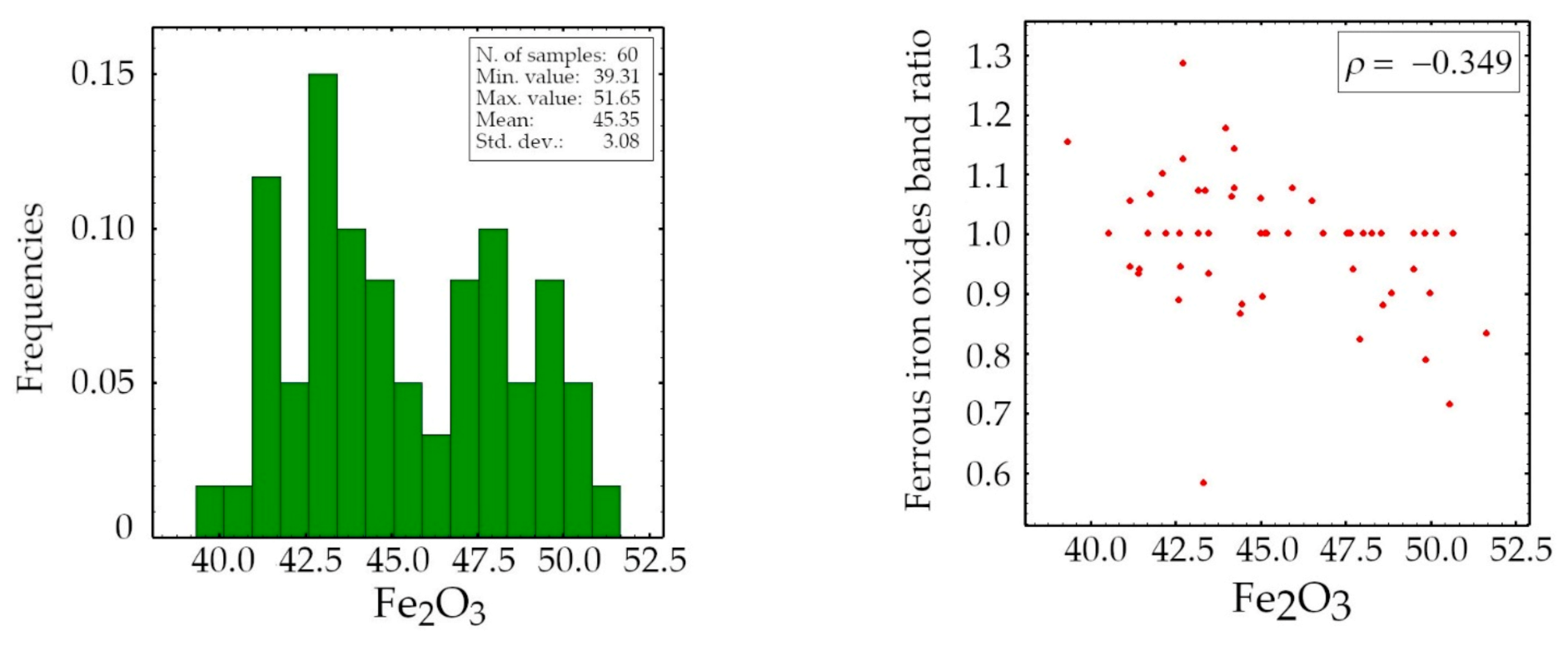
| Ferrous iron oxides | −0.349 | |
| Ferric Iron, Fe3+ | −0.150 | |
| Ferrous Iron, Fe2+ | 0.194 | |
| Ferrous silicates | −0.125 | |
| Ferric oxides | 0.223 |
| Fe2O3 (%) Variogram Models | ||||
|---|---|---|---|---|
| Nugget Effect | Spherical 1 | Spherical 2 | ||
| Range (m) | Sill | Range (m) | Sill | |
| 2.3 | 70 | 2.9 | 180 | 3.4 |
| Direct variable—Fe2O3 (%)—Variogram Models | ||||
| Nugget Effect | Spherical 1 | Spherical 2 | ||
| Range (m) | Sill | Range (m) | Sill | |
| 2.3 | 70 | 2.9 | 180 | 3.4 |
| Auxiliary Variable—Band Ratio—Variogram Models | ||||
| Nugget Effect | Spherical 1 | Spherical 2 | ||
| Range (m) | Sill | Range (m) | Sill | |
| 0.0027 | 70 | 0.0063 | 180 | 0.011 |
| Cross-Variogram Models | ||||
| Nugget Effect | Spherical 1 | Spherical 2 | ||
| Range (m) | Sill | Range (m) | Sill | |
| 0 | 70 | −0.116 | 180 | 0.0001 |
| Fe2O3 (%) Variogram Models | ||||
|---|---|---|---|---|
| Nugget Effect | Spherical 1 | Spherical 2 | ||
| Range (m) | Sill | Range (m) | Sill | |
| 2.3 | 70 | 2.9 | 180 | 3.4 |
| Band Ratio-Component 1 Variogram Models | ||||
| Spherical 1 | ||||
| Range (m) | Sill | |||
| 70 | 0.0063 | |||
| Cross-Variogram Models | ||||
| Spherical 1 | ||||
| Range (m) | Sill | |||
| 70 | −0.116 | |||
Publisher’s Note: MDPI stays neutral with regard to jurisdictional claims in published maps and institutional affiliations. |
© 2021 by the authors. Licensee MDPI, Basel, Switzerland. This article is an open access article distributed under the terms and conditions of the Creative Commons Attribution (CC BY) license (https://creativecommons.org/licenses/by/4.0/).
Share and Cite
Bruno, R.; Kasmaeeyazdi, S.; Tinti, F.; Mandanici, E.; Balomenos, E. Spatial Component Analysis to Improve Mineral Estimation Using Sentinel-2 Band Ratio: Application to a Greek Bauxite Residue. Minerals 2021, 11, 549. https://doi.org/10.3390/min11060549
Bruno R, Kasmaeeyazdi S, Tinti F, Mandanici E, Balomenos E. Spatial Component Analysis to Improve Mineral Estimation Using Sentinel-2 Band Ratio: Application to a Greek Bauxite Residue. Minerals. 2021; 11(6):549. https://doi.org/10.3390/min11060549
Chicago/Turabian StyleBruno, Roberto, Sara Kasmaeeyazdi, Francesco Tinti, Emanuele Mandanici, and Efthymios Balomenos. 2021. "Spatial Component Analysis to Improve Mineral Estimation Using Sentinel-2 Band Ratio: Application to a Greek Bauxite Residue" Minerals 11, no. 6: 549. https://doi.org/10.3390/min11060549