
Investigation of Surface Residual Stress for Medium Carbon Steel Quenched by YAG Laser with Extended Cycloidal Motion


1
Department of Mechanical Engineering, Center for Environmental Toxin and Emerging-Contaminant Research, Super Micro Mass Research & Technology Center, Cheng Shiu University, Kaohsiung 833301, Taiwan
2
Department of Industrial Upgrading Service, Metal Industries Research & Development Center, Kaohsiung 811020, Taiwan
*
Author to whom correspondence should be addressed.
Metals 2022, 12(11), 1903; https://doi.org/10.3390/met12111903
Submission received: 17 October 2022
/
Revised: 3 November 2022
/
Accepted: 4 November 2022
/
Published: 7 November 2022
(This article belongs to the Special Issue Advances in Metallic Heat Treatment and Surface Engineering)
Abstract
:This study investigated the surface residual stress for AISI 1045 steel quenched by a YAG laser. A coaxial laser spindle was installed on a CNC machine for the experiment. The laser motion was arranged to follow the path of an extended cycloid which widened the quenching area on the steel surface. Both the temperature distribution and the residual stresses were measured by thermocouples and a portable X-ray diffractometer, respectively. When the temperature distribution was cooled down near the value of the room temperature, the residual stresses were then measured after the laser quenching process. The diffractometer used a single exposure of X-ray with a two-dimensional detector to calculate the Debye–Scherrer ring (D-S ring) for the determination of the normal and shear stresses. Different laser powers were exploited for the measurement of residual stresses, including 500, 600, 700, and 900 watts. In addition to the experiment, an analytic model for the investigation of residual stresses was built by the finite element analysis for which MSC Marc was used. The assumption for the FEA was that the laser spot had a circular shape of uniform energy distribution and the thermal–elastic–plastic model was applied to the simulation for the laser quenching process. The analytic and experimental results for the surface residual stresses had excellent consistency with a maximum difference of 10.5% from the normal stresses. The numerical results for the residual stresses also revealed that the normal stresses were compressive for the laser-quenching treatment and the shear stress could be neglected compared to the normal stress.
1. Introduction
In modern industry, a laser is a powerful tool for fine manufacturing. The surface heat treatment of metallic elements or structures by laser is one example. The laser spot has a high-power density which induces the effect of rapid heating and cooling on the heat-affected zone (HAZ). The quenching feature of a laser is that the manipulation of localized and specific heat treatment can be applied to mechanical elements with complex contours, such as gears, cams, crankshafts, etc. Various metallic materials have been studied for the surface heat treatment by laser. In 2008, Lakhkar et al. published an article about the multitrack laser hardening of AISI 4140 steel [1]. Using 42CrMo cast steel, the hardening thickness with a laser treatment was investigated by Sun et al. in 2014 [2]. In 2015, Barka and Ouafi analyzed the process parameters for AISI 4340 treated by laser hardening [3]. For the purpose of a wide quenching treatment, the overlapping operation between the laser spot and the heat-affected zone was arranged to reduce the variation of the hardening depth. In 2018, Hung et al. studied the effects of the various laser scan paths on the temperature distribution and the surface hardness of AISI 1045 steel [4,5]. In those studies, the YAG laser was mounted on a CNC machine and programmed to follow a linear scan path [4] and an extended cycloidal path by which the quenching area was widened [5]. The results from Hung’s studies showed that the hardness of the laser-quenched surface varied with respect to the temperature field variation on which the laser input power and scan path had a strong influence. Instead of the conventional quenching and tempering treatment, Espinoza et al. studied a laser application for the surface heat treatment of 1538 MV steel [6]. The deterioration by oxidation was studied for the laser quenching process by N. Maharjan et al. [7]. In that study, the gas atmosphere was controlled to prevent the generation of oxide, and the result showed that the laser-quenching effects were enhanced. Instead of a steel plate, R. Fakir et al. studied cylindrical specimens of AISI 4340 treated by the laser quenching process [8,9]. In the study [8], an analysis by the finite difference and finite element methods was validated by experimental results with respect to the temperature distribution. Following the validation study, a servocontrol was applied for the laser quenching process to investigate the case depth [9]. Chen et al. studied the effect of the impact of abrasive wear on the surface by laser quenching for 40Cr steel [10]. In addition to its powerful tooling capability, the laser has also revealed its potential for affecting the ESG index. ESG stands for environment, society, and governance. Traditionally, the machining of Inconel 718 is operated by a ceramic tool which operates slowly, costs a lot of cutting fluid, and needs much electric power consumption. In the study by Pan et al. [11], a milling machine was equipped with a laser. In the study, the milling of Inconel 718 was transformed into an effective operation in which the workpiece surface was annealed by laser in advance. With the laser preoperation, the milling tool cut the workpiece easily, quickly, and economically.
In spite of its outstanding features as a powerful tool for mechanical manufacturing, the laser surface treatment has an intrinsic problem related to the residual stress induced in the quenching process. Fatigue and fracture failures are often attributed to residual stresses [12,13]. As a destructive measurement, the hole-drilling method was popular in the industry for the measurement of residual stress. In the method, a drilling hole is applied to the specimen, and the strains and displacements are measured by strain gauges. The corresponding residual stress is then calculated [14,15]. In 2021, Peng et al. used the digital image correlation (DIC) approach combined with the blind-hole drilling method for the measurement of residual stresses [16]. Instead of using strain gauges, ink marks were applied on the workpiece surface and analyzed in the measurement process. In addition, the parameters’ formulae for the evaluation of residual stresses were obtained by a finite element analysis. It showed that the result of the DIC–hole drilling method had excellent consistency with the theoretical values and the result of the hole drilling method. As an alternative, X-ray diffraction by crystals has been proposed for the measurement of the residual stresses. The and methods are often used for the residual stress measurement by X-ray diffraction. In the method, the tilt angle, , of the X-ray incidence is measured for several positions. The plot, the lattice strain vs. , is built and the slope is used to find the corresponding stress [17]. Using the Debye–Scherrer ring (D-S ring), the method provides another feasible measurement by X-ray diffraction for the residual stress determination [17]. In 1978, Taira, Tanaka and Yamasaki laid the foundation for the method [18]. Tanaka extended the technology of the method for the measurement of triaxial residual stress in 2018 [19]. In 1989, Yang and Na used a finite element analysis to simulate the transient thermal stress and the residual stress for carbon steel quenched by laser for the two-dimensional case [20]. H. Köhlera used neutron diffraction to evaluate the residual stress distribution of materials due to fatigue [21]. In 2013, P. Ganesh studied the microstructural characterization of the laser hardening process for AISI 1045 steel [22]. For steel quenched by laser, it showed that the internal stress variation under long-term reversal loads induced the damage by fatigue. Liverani et al. used a numerical analysis to calculate the residual stress for an AISI 9180 steel cam [23]. For validation, the XSTRESS 3000 diffractometer with a standard Cr-tube radiation source, was used to measure the residual stress. It showed that the incident laser energy density and scanning speed had strong effects on the surface hardness and the hardening depth.
In reference [24], the surface hardness and the corresponding hardening depth were studied for AISI 1045 steel quenched by laser with power values of 2500 and 5000 W. However, in the study, the temperature distribution and the corresponding residual stresses were not discussed. Due to the laser application in local area quenching, the destructive measurements of residual stresses are seldom used. In this study, the residual stresses and the corresponding temperature distribution are studied for AISI 1045 steel quenched by laser. The laser scanning path follows an extended cycloidal curve which widens the quenching area on the steel surface. FEA software MSC Marc is exploited to build the analytic model for the simulation of the temperature distribution and the determination of the residual stresses. To validate the results of the FEA simulation, the temperatures and the residual stresses are measured by thermocouples and the PULSTEC μ-X360n portable X-ray diffractometer, respectively. The D-S rings are shown and used to calculate the residual stress, which includes the normal stress and the shear stress.
2. Finite Element Modeling
In this study, the surface residual stresses by the laser quenching process were analyzed for AISI 1045 steel. FEA software MSC Marc was used for the simulation. The material properties of AISI 1045 steel are listed in Table 1 [25]. In the table, the parameters, including thermal conductivity, specific heat, and Young’s modulus, are temperature-dependent, as shown in previous research by the authors [5].
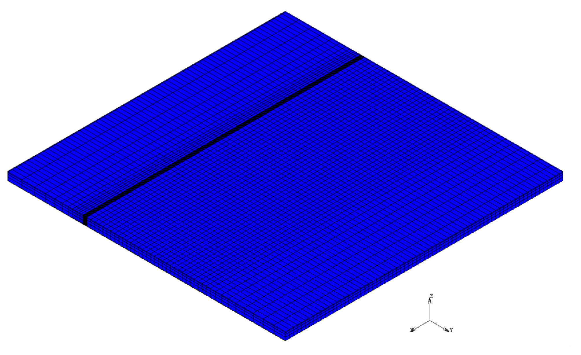
The mesh model for the specimen is shown in Figure 1 [5]. The dimensions of the specimen were 70 mm × 70 mm × 2 mm in the simulation. The quenching process by laser followed the principal rules related to the coupled thermal–mechanical model. Using MSC. Marc (MSC Software, Newport Beach, CA, USA), the thermos-elastic–plastic model was applied for the simulation. Following the von Mises criterion, the flow and isotropic strain hardening rules can be expressed as:
where is the deviatoric reduced stress tensor, is the effective stress, and is the effective plastic strain.
The definition of is written as:
If the influence of the temperature variation is considered, Equation (1) can be rewritten as:
where G is the modulus of rigidity and α stands for the thermal expansion coefficient.
In the simulation, the residual stresses after the laser quenching operation were extracted when the temperature of the specimen was cooled down at the value of the ambient temperature, 25 °C in this study.
2.1. Governing Equations for Heat Transfer
In the simulation of the laser quenching process, the heat transfer mechanisms included heat conduction, heat convection, and the external heat source by the laser power. The effect of heat radiation was neglected in the simulation. The heat conduction is governed by Fourier’s law, as shown below,
where is the heat flow rate inside the material, is the area through which the heat flow rate passes in the direction of the area normal, is the heat conductive coefficient, and is the temperature variation across the area . Based on the assumption of no mass transfer and the principle of energy conservation, the temperature in the material body must satisfy the following equation,
where is the volumetric heat source, is the material density, is the specific heat, respectively. On the boundary in the simulation, the heat transfer mechanism was governed by convection and the equation for the natural heat convection can be expressed as
where is the heat flow rate by natural convection, is the natural heat convection coefficient, and is the ambient temperature. In the simulation, the initial temperature of the material had a value of 25 °C, and the heat convection coefficient was assumed to be 12.6 W/m2·°C. In the FEA simulation, the temperature-dependent parameters were assumed to be constant, as well as those of the temperature over the melting point. The heat transfer mechanisms were only used as a macro view for the simulation. As a micro view, the residual stresses should be attributed to the martensitic transformation with a volume expansion.
2.2. Laser Power Simulation
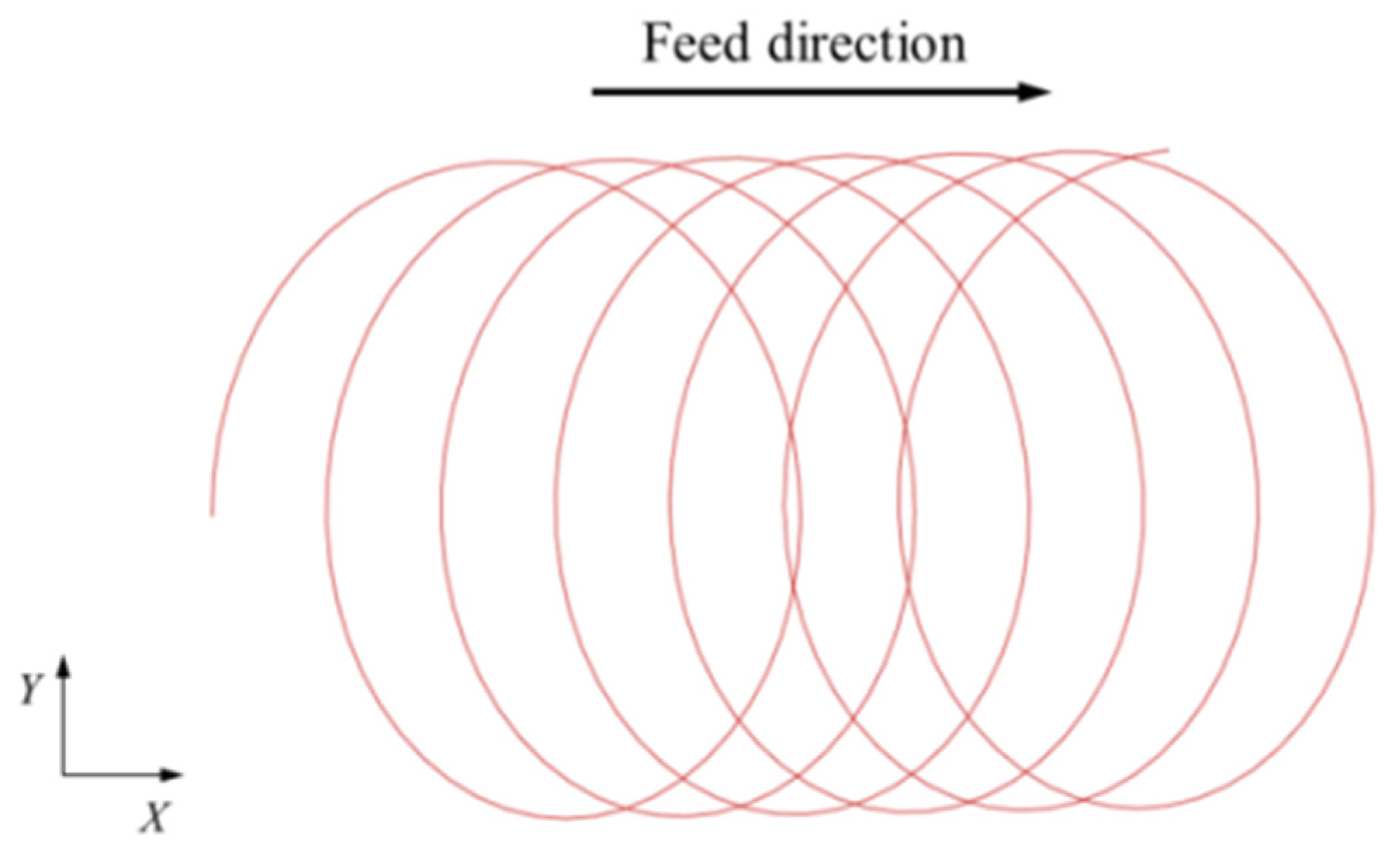
The CNC milling machine was equipped with a coaxial laser-assisted spindle. The operation of the laser heat source moved circularly around a center which translated linearly along the surface of the specimen, as shown in the Figure 2.
The moving path was referred to as the extended cycloidal curve, which was used to widen the quenching area affected by the laser heat source. In the simulation, the subroutine of the language, Fortran, was programmed for the moving laser to heat on the boundary. In addition, the laser power was assumed to be uniform on the surface of the specimen affected by the laser spot [5]. The mathematical formula for the power intensity absorbed by the specimen can be written as
where is the average magnitude of the laser power, is the absorption rate of the specimen, and is the radius of the laser spot. In the subroutine, the extended cycloidal curve was used for the path for the center of the laser spot, which was programmed to be a circle of radius with power intensity . In this study, , the thermal absorption rate for the specimen, had a value of 35% [5].
3. Experimental Setup
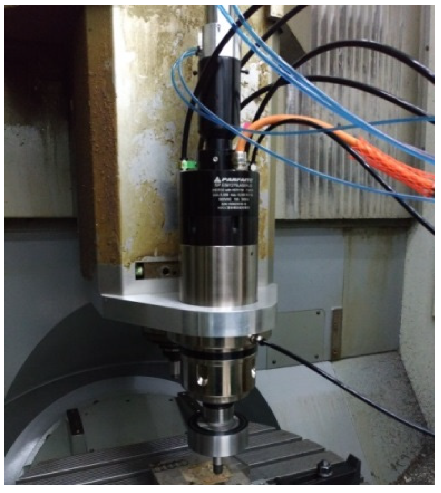
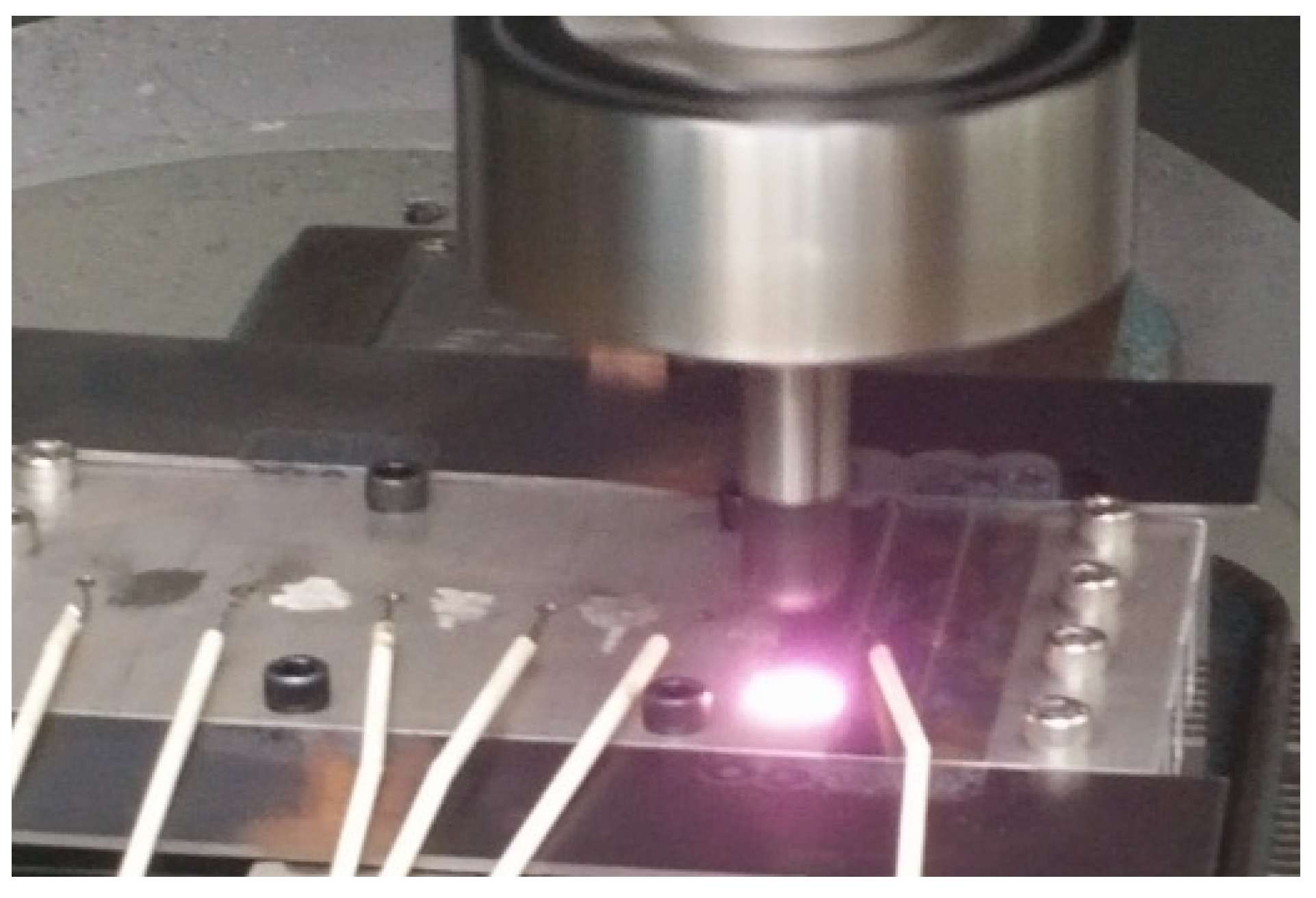
In Figure 3, the coaxial laser-assisted spindle of the CNC machine is shown. The laser source used a laser diode which had a wavelength of 976 ± 1 nm. The maximum power of the laser had the value of 1500 W. The CNC was equipped with a water-cooling module. In the experimental setup, the thermocouples were arranged to measure the temperature variation on the different positions of the specimen. The arrangement of the thermocouples is shown in Figure 4. The laser spot from the figure had a diameter of 2 mm in the actual operation when the laser was correctly focused. Along the extended cycloidal path, the laser spot moved at a circular speed of 100 rpm around the point which moved with a linear speed of 100 mm/min along the x-axis, as shown in Figure 2.
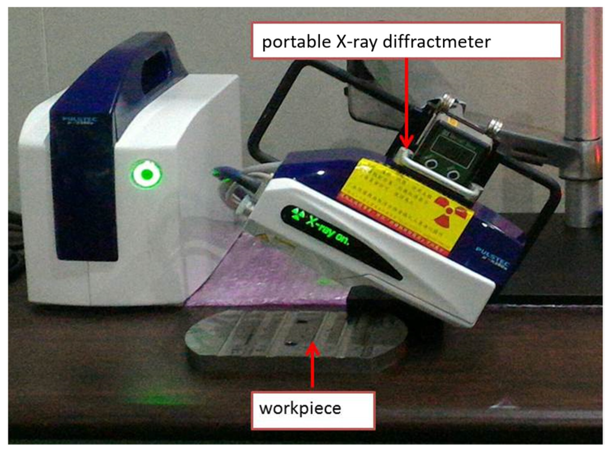
As shown Figure 5, the residual stress measurement was measured by the PULSTEC μ-X360n portable X-ray diffractometer.
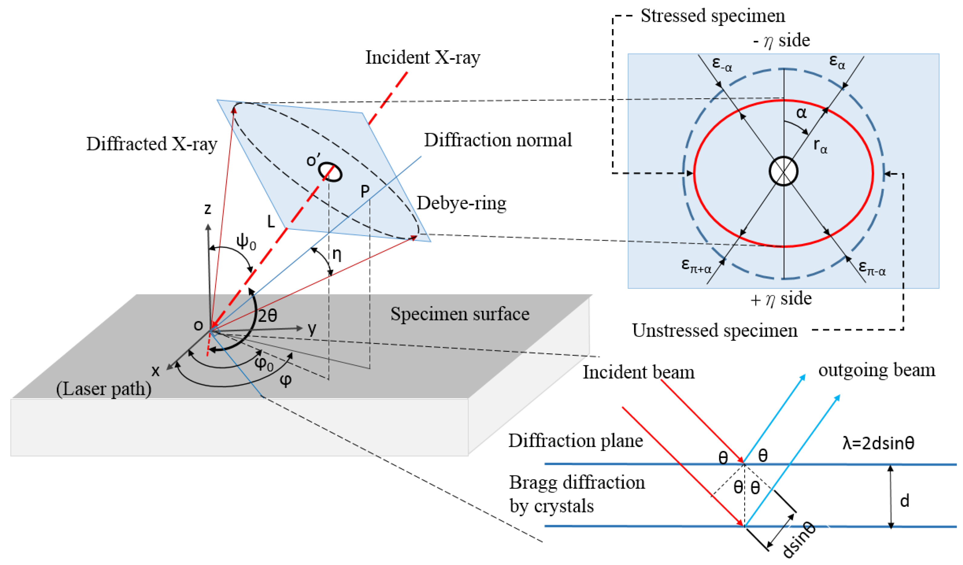
The portable X-ray diffractometer used a single X-ray tube as its emitting source and a two-dimensional detector for the imaging of Debye–Scherrer ring (D-S ring). The stress-free sample data were stored in the X-ray diffractometer, which could generate the stress-free D-S ring. When the workpiece was machined, the D-S ring measured by the X-ray diffractometer changed. The variation of the D-S rings between the stress-free data and the measured data for the machined workpiece showed the values of strain and the corresponding stresses could be derived. The stresses measured by the portable X-ray diffractometer included normal stress and shear stress. In this study, the normal stress, , had its normal in the X-axis direction as shown in Figure 2. The following describes the principles of the X-ray diffractometer [17]. The schematic illustration for the measurement by the X-ray diffractometer is shown in Figure 6.
In Figure 6, the reference planes include the specimen surface with the Z-axis as normal, the imaging plane (IP) with the incident X-ray as normal, and the diffraction planes which are constructed by the polycrystal structure of the specimen. The angle, , is the one between the diffraction normal and the incident X-ray. The angle between the diffraction plane and the incident X-ray is the diffraction angle , satisfying the following equation.
The Bragg formulation of the X-ray is satisfied for the crystalline specimen, and the distance between the diffraction planes is denoted by and is as follows:
where is the wavelength of the X-ray. Using Equation (9), the relationship between and is derived and the corresponding strain is written as
where and are the values for the stress-free state, and and denote the measured data for the specimen after machining, respectively. In Figure 6, the distance between the point on the IP plane and the origin on the specimen surface is denoted by . The image by X-ray diffraction on the imaging plane is referred to as the D-S ring. The distance varies according to the angle, as shown in Figure 6. The following equation is written in terms of the diffraction angle , the radius on IP, and the length .
Using Equations (10) and (11), the strain can be derived as
where is the radius of the stress-free D-S ring. Let be the average value of the D-S ring. The length in Equation (12) is then approximated by the following equation,
where is the angle between the X-ray incidence and the diffraction normal in the stress-free state. In terms of , and , the following equations are used to define the strains and .
When , Equations (16) and (17) can be written in terms of and , as shown below. A detailed discussion can be found in reference [17].
where and are Young’s modulus and Poisson’s ratio, respectively. As shown in Figure 2, the laser’s moving path and the X-Y plane defined on the specimen surface are described. In addition, the linear relation between and is used to calculate in terms of the slope . Similarly, can be estimated by the slope . Equations (18) and (19) can be written as below.
where
and
where
In this study, the parameters for the portable X-ray diffractometer are listed in Table 2.
From the table, we see that the X-ray spot had a diameter of 5 mm. The incidence angle of the X-ray was and the valid range of angle was from to .
4. Numerical Results and Discussion
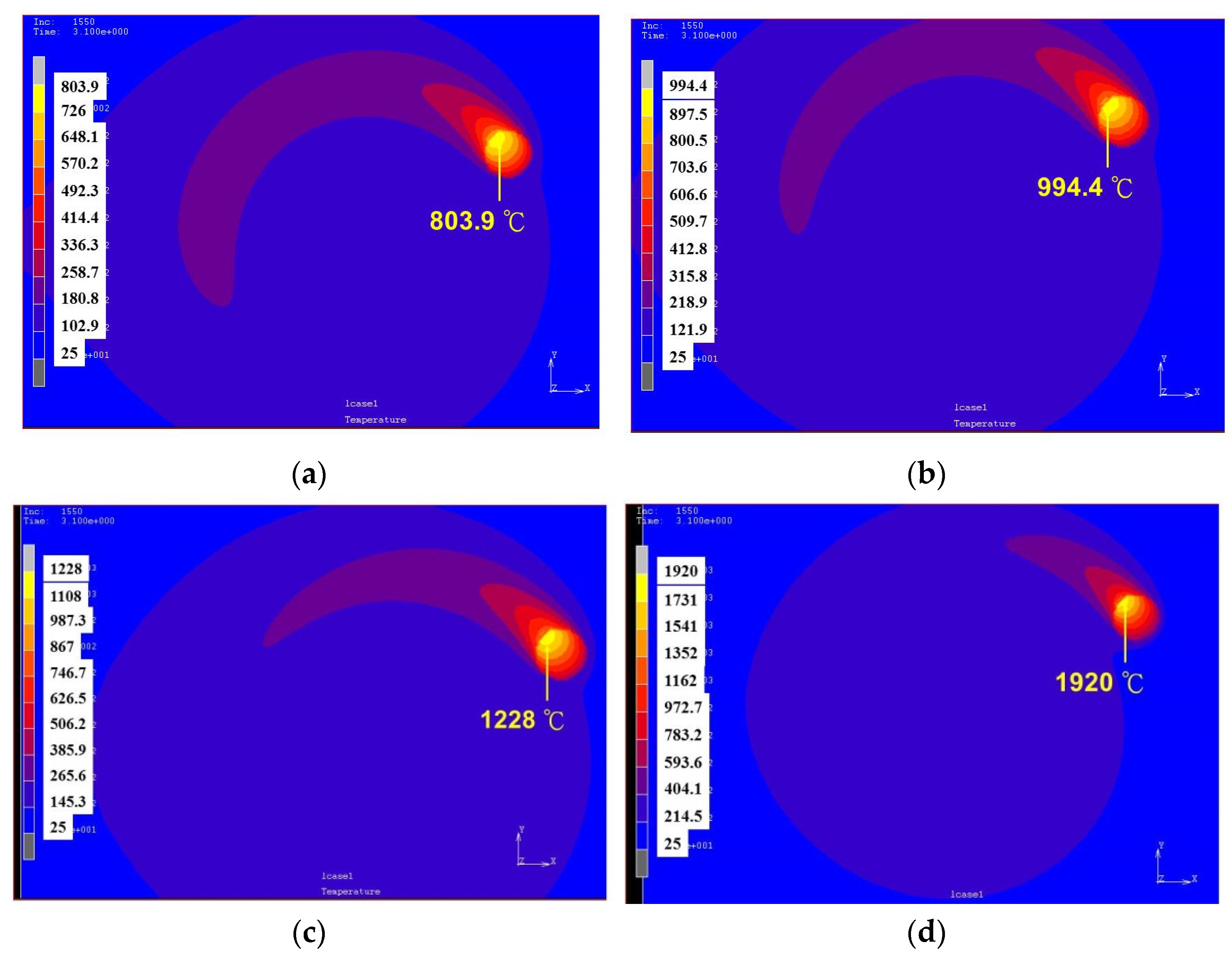
In Figure 7, the laser quenching processes are shown for the different laser powers, including 500 W, 600 W, and 700 W [5]. In the process, the laser spot followed an extended cycloidal curve which had a linear speed of 100 mm/min and a rotational speed of 100 rpm. The laser spot had a diameter of 2 mm and rotated at a radius of 7 mm. Using the extended cycloidal path, the area affected by the laser heating was controllable on a wide scale. The numerical results by the FEA showed that the core temperatures around the laser spot area were above 800 °C and reached the austenitizing temperature. It was concluded that the surface zone with a temperature of 760 °C or over was hardened in the heating process.
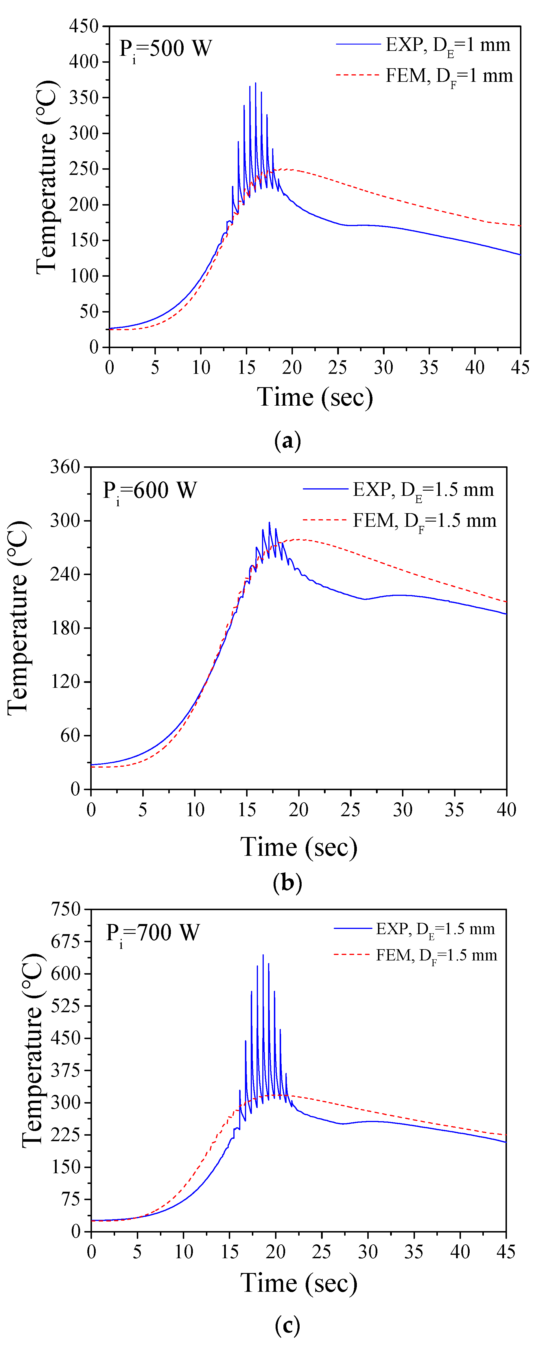
The numerical results of the temperature variation by the FEA and measurements are shown in Figure 8. According to the arrangement of the thermocouples as shown in Figure 4, the measuring point of the temperature was located at the distances of 1 mm and 1.5 mm away from the laser spot. At a laser power of 900 W, it was found that the thermocouple couple lost its contact at the welding point for which the comparison chart is not portrayed. In Figure 8, according to the FEA results at the measuring position, the maximum temperatures were around the values of 240 °C, 275 °C, and 315 °C for laser powers of 500 W, 600 W, and 700 W, respectively. For the experimental results, the temperature variation was vigorous when the laser spot was around the measuring point. The difference between the FEA and experimental results may be attributed to the distance between the measuring point and captured measurement data frequency. The experimental and simulated captured frequencies were 300 Hz and 100 Hz, respectively. The acquisition frequency was reduced during the simulation to reduce the huge quantity of data and save computing time. Therefore, the temperature field results obtained were relatively smooth. The experimental data showed that the temperature increased when the laser approached the measurement point and decreased when it moved away. According to the experimental results, as shown in Figure 8a,b, the maximum temperatures were 370 °C and 300 °C for the a laser power of 500 W with an offset of 1 mm and 600 W with an offset of 1.5 mm, respectively. In addition, as shown in Figure 8b,c, the maximum temperatures were 300 °C and 640 °C for laser powers of 600 W and 700 W with the same offset of 1.5 mm. The experimental results showed that the maximum temperature in the vigorous variation region was strongly affected by the laser power and the offset between the thermocouple and the laser spot.
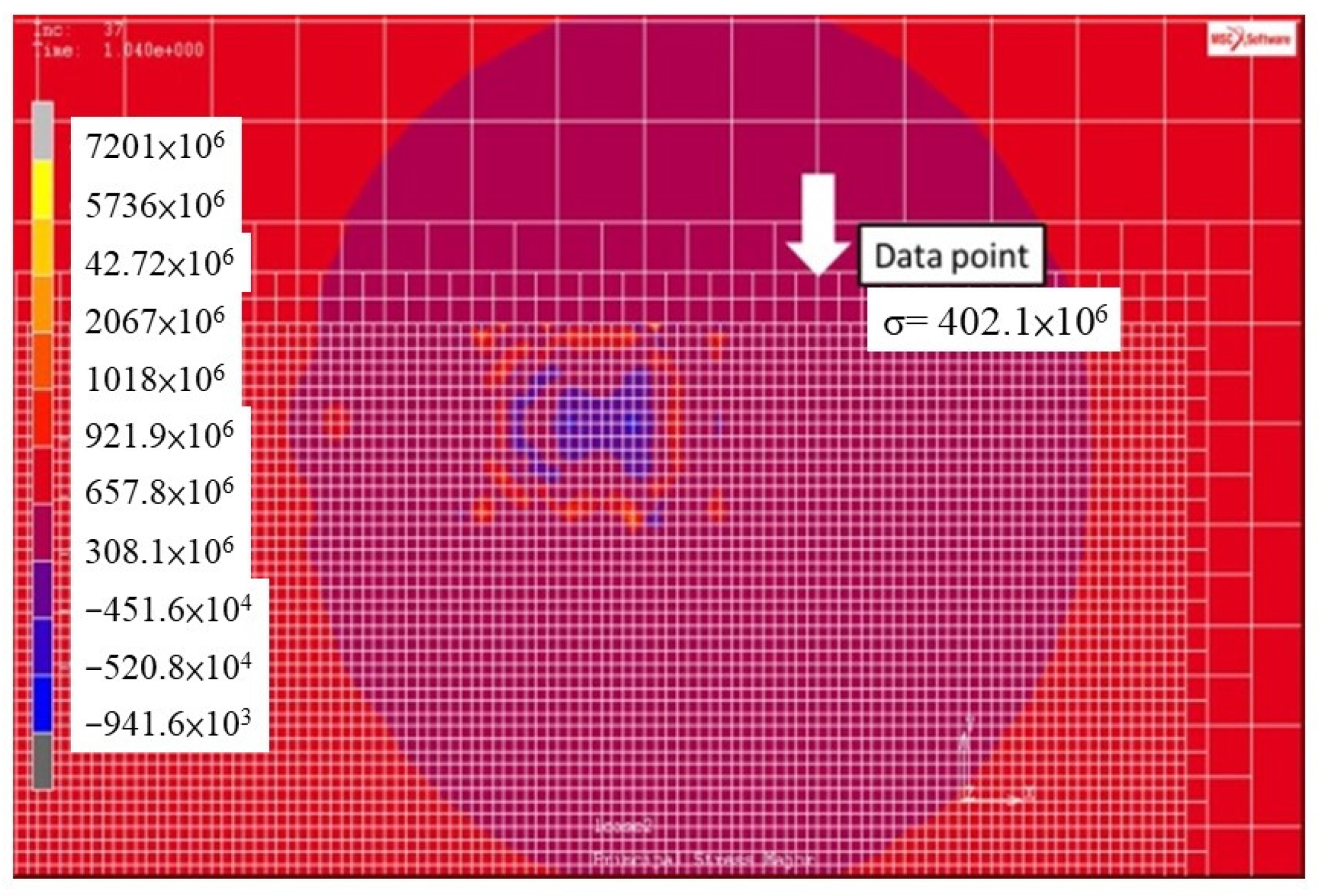
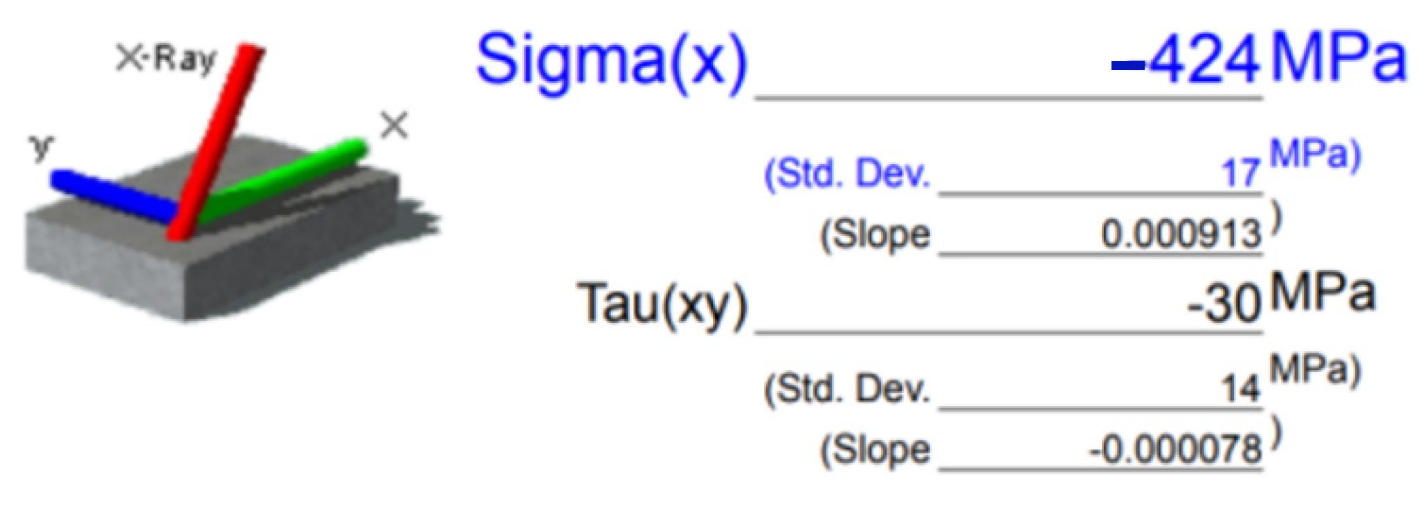
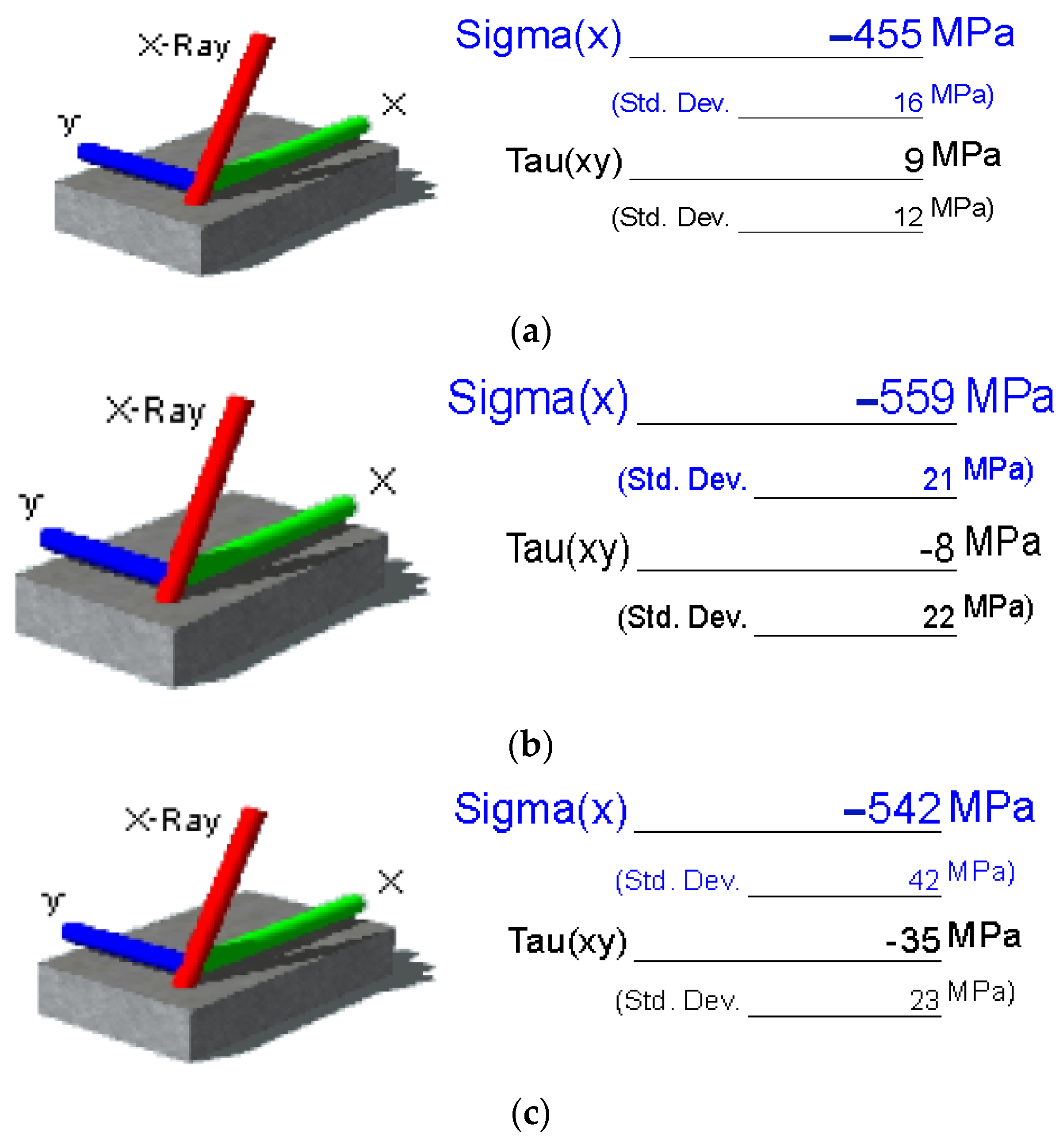
With the extended cycloidal path of the laser spot, the residual stress prediction in the laser-hardened zone is shown in Figure 9. In the figure, the laser power had a value of 500 W. The extended cycloidal movement had a linear speed of 100 mm/min and a rotational speed of 100 rpm. According to the simulation, the normal stress with the normal as the X-axial direction was compressive and had a value of 402.1 MPa. Using the PULSTEC μ-X360n diffractometer (Pulstec Industrial Co., Ltd., Hamamatsu, Japan), the residual stresses measured had a normal stress of −424 MPa and a shear stress of −30 MPa, as shown in Figure 10.
The stress-free data for AISI 1045 steel logged in the portable X-ray diffractometer are listed in Table 3.
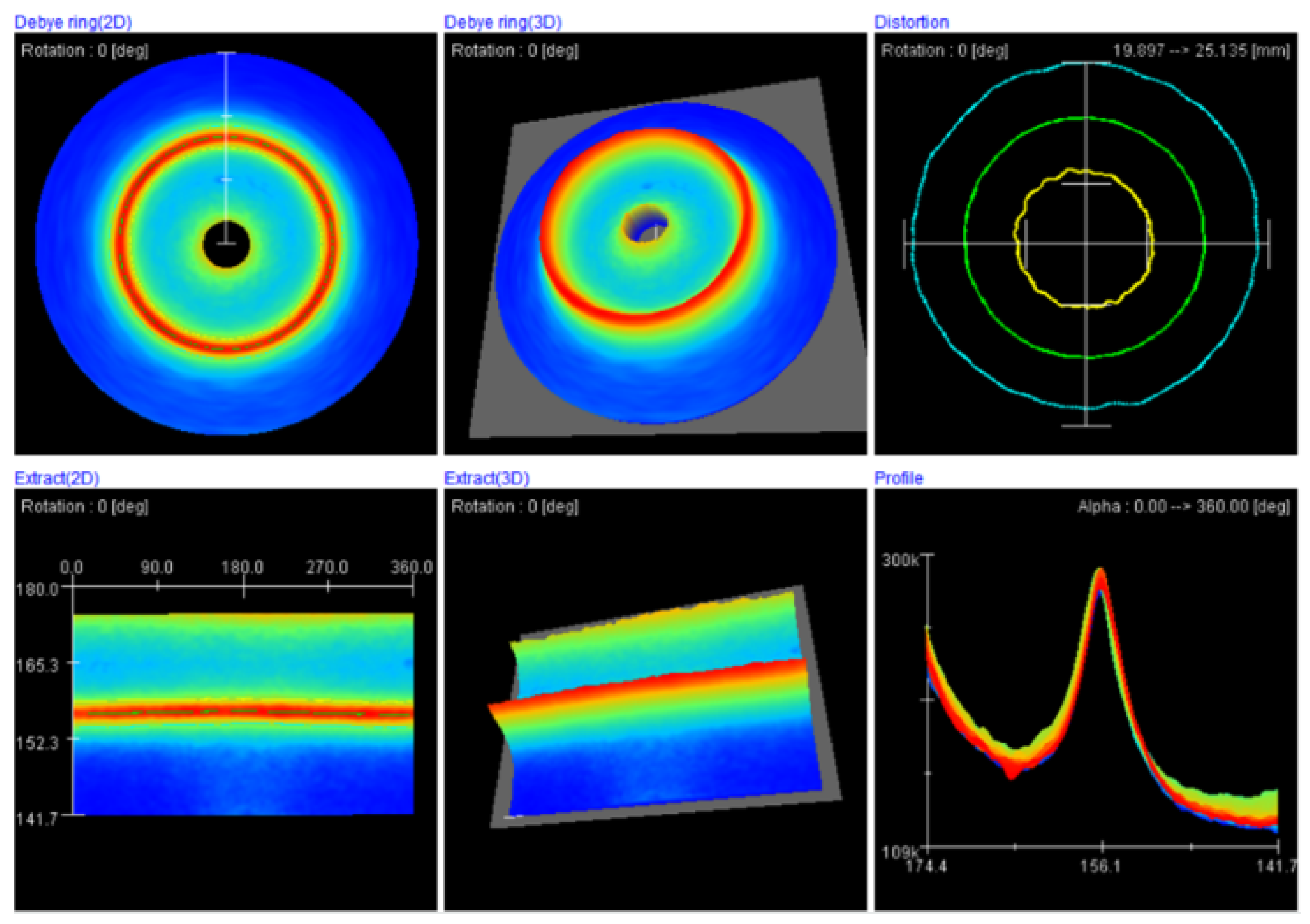
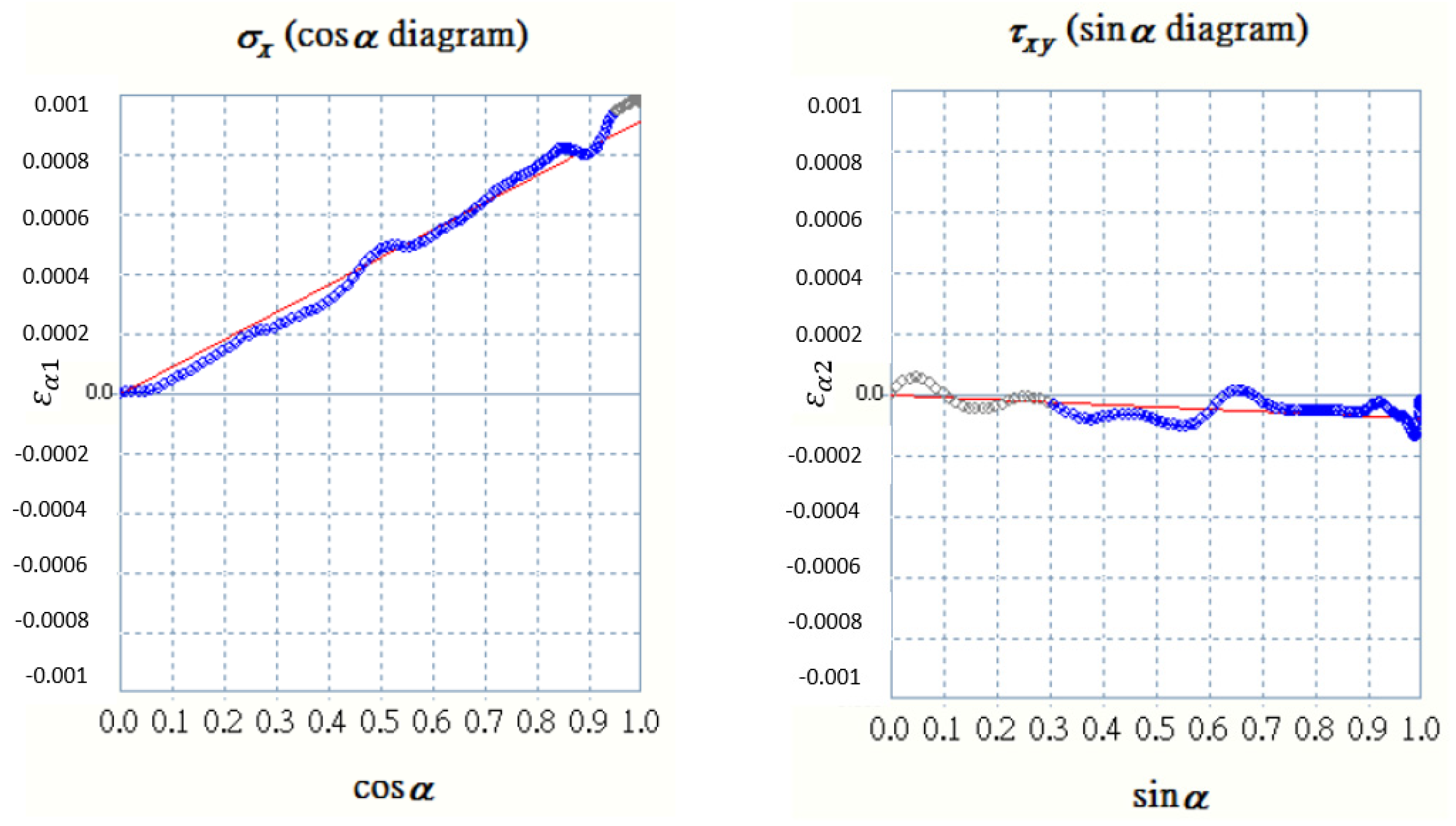
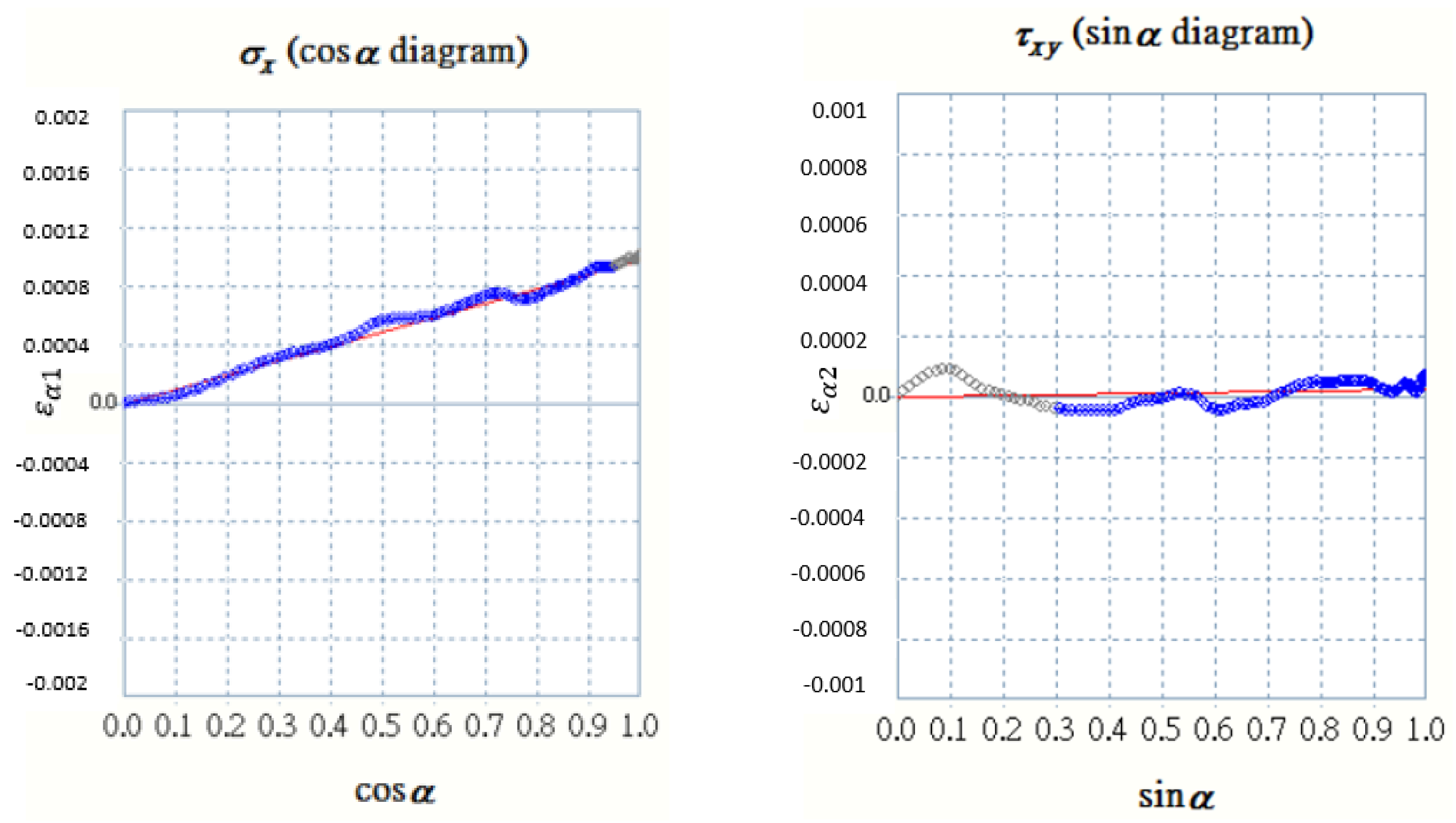
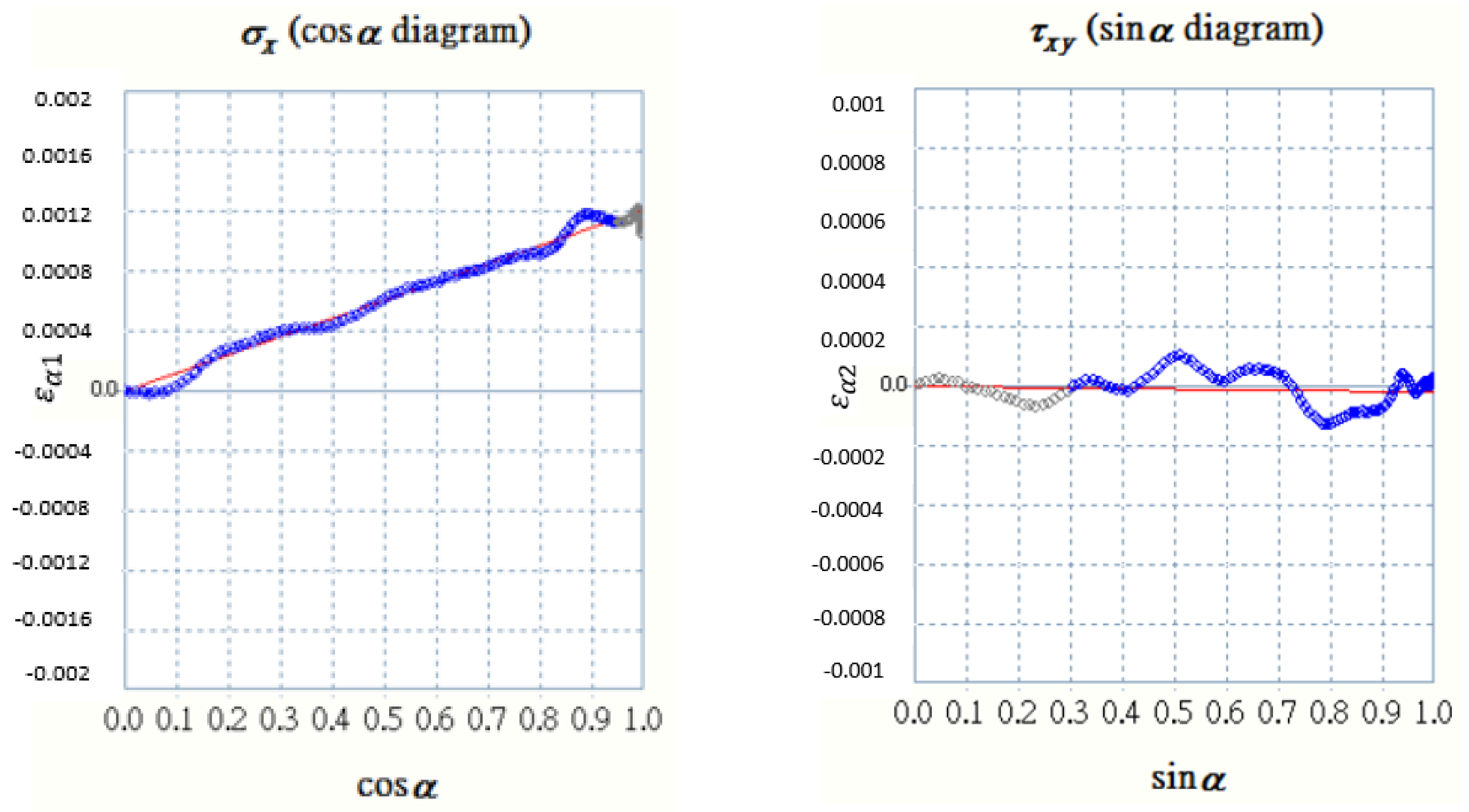
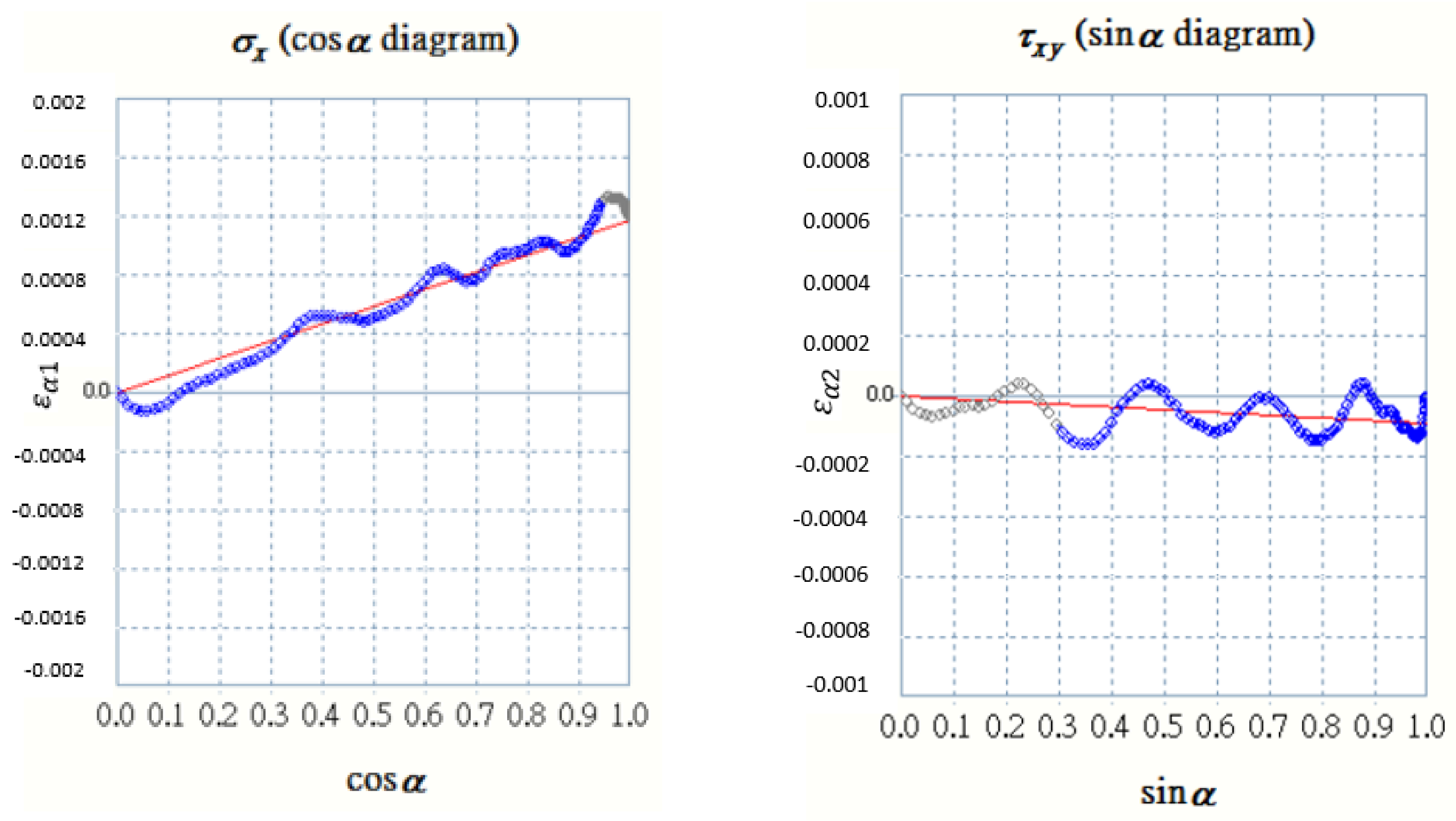
The detailed information about the corresponding D-S ring is shown in Figure 11 for the specimen quenched by a laser power of 500 W. In this figure, the 2D and 3D images of the D-S ring are shown, and the corresponding extract images are arranged below. The third column list the distortion and the radial cross section’s profile of the D-S ring. Figure 12 shows the plots of () and . The slopes of these two plots are shown in Equations (21) and (24), and the corresponding stresses can be calculated by Equations (19) and (22), as shown in Figure 10. In Figure 12, it is observed that a positive slope means a negative value for the normal stress, and a negative slope corresponds to a negative value for the shear stress, as shown in Equations (20) and (23). The plots of () and are shown for the laser quenching processes at 600 W, 700 W, and 900 W in Figure 13, Figure 14 and Figure 15.
According to the calculation of the slopes in Figure 13, Figure 14 and Figure 15, the measurements of the residual stresses are shown in Figure 16.
It is observed that the absolute value of the shear stress was far less than that of the normal stress. In Table 4, the numerical results of the normal stresses are listed for the experimental measurement and the simulation. According to the results, the experimental results had good consistency with the ones of the simulation, and the maximum deviation of the normal stresses was 10.5% when the laser power was 600 W.
The residual stresses, as a micro view, should be attributed to the martensitic transformation with a volume expansion. It was found that the maximum hardness was 534 HV for a laser power of 500 W [5]. The heating temperature should be over the Ac3 point to obtain the martensite of steel. The Ac3 point was assumed to be 760 °C in the simulation. According to Figure 7, the temperatures of the laser spot were over 760 °C. It indicated that the martensitic transformation occurred on the steel surface.
5. Conclusions
In this study, the residual stress induced by the laser quenching process was investigated for AISI 1045 steel. Using FEA software MSC Marc, the thermoelastic–plastic model was applied to the meshing model in the simulation. In the experimental setup, a CNC milling machine equipped with a coaxial laser-assisted spindle had an operational path as an extended cycloidal curve which was programmed to widen the quenching area on the specimen. When the temperature of the specimen was quenched by laser and cooled down around the ambient temperature, the residual stresses were measured by the PULSTEC μ-X360n X-ray diffractometer. According to the experimental results, the absolute values of the shear stresses were far less than those of the normal stresses. The numerical results of the normal stresses were analyzed for the experimental measurement and the simulation. It showed that the minimum and maximum deviations of the normal stress were 3.32% and 10.5% for laser powers of 900 W and 600 W, respectively. According to the analysis, the results of the simulation in this article had a good consistency with those of the temperature and residual stress measurements. It reveals that the proposed model can be used to simulate the laser quenching process for carbon steel mechanical elements with complex contours, such as gears, cams, crankshafts, etc. The corresponding temperature variation and residual stress distribution can be predicted in advance.
Author Contributions
Conceptualization: T.-P.H.; Data curation: H.-A.T.; Methodology: T.-P.H. and A.-D.L.; Software: H.-A.T.; Validation: T.-P.H. and H.-A.T.; Experimental work: H.-A.T. and A.-D.L.; Writing—review and editing: T.-P.H.; Supervision: A.-D.L.; Funding acquisition: H.-A.T. All authors have read and agreed to the published version of the manuscript.
Funding
This research was funded by the Metal Industries Research and Development Centre (MIRDC), grant number 11D5218225.
Data Availability Statement
Data available on request from the authors.
Conflicts of Interest
The authors declare no conflict of interest.
References
- Lakhkar, R.S.; Shin, Y.C.; Krane, M.J.M. Predictive modeling of multi-Track laser hardening of AISI 4140 steel. Mater. Sci. Eng. A 2008, 480, 209–217. [Google Scholar] [CrossRef]
- Sun, P.; Li, S.; Yu, G.; He, X.; Zheng, C.; Ning, W. Laser surface hardening of 42CrMo cast steel for obtaining a wide and uniform hardened layer by shaped beams. Int. J. Adv. Manuf. Technol. 2014, 70, 787–796. [Google Scholar] [CrossRef] [Green Version]
- Barka, N.; El Ouafi, A. Effects of laser hardening process parameters on case depth of 4340 steel cylindrical specimen—A statistical analysis. J. Surf. Eng. Mater. Adv. Technol. 2015, 5, 124–135. [Google Scholar] [CrossRef] [Green Version]
- Hung, T.; Shi, H.; Kuang, J. Temperature modelling of AISI 1045 Steel during Surface Hardening Processes. Materials 2018, 11, 1815. [Google Scholar] [CrossRef] [PubMed] [Green Version]
- Hung, T.; Hsu, C.; Tsai, H.; Chen, S.; Liu, Z. Temperature field numerical analysis mode and verification of quenching heat treatment using carbon steel in rotating laser scanning. Materials 2019, 12, 534. [Google Scholar] [CrossRef] [Green Version]
- Carrera-Espinoza, R.; Valerio, R.; Villasana, J.D.; Hernandez, J.A.Y.; Moreno-Garibaldi, P.; Cruz-Gomez, M.A.; Lopez, U.F. Surface laser quenching as an alternative method for conventional quenching and tempering treatment of 1538 MV steel. Adv. Mater. Sci. Eng. 2020, 2020, 7950684. [Google Scholar] [CrossRef] [Green Version]
- Maharjan, N.; Zhou, W.; Wu, N. Direct laser hardening of AISI 1020 steel under controlled gas atmosphere. Surf. Coat. Technol. 2020, 385, 125399. [Google Scholar] [CrossRef]
- Fakir, R.; Barka, N.; Brousseau, J. Case study of laser hardening process applied to 4340 steel cylindrical specimens using simulation and experimental validation. Case Stud. Therm. Eng. 2018, 11, 15–25. [Google Scholar] [CrossRef]
- Fakir, R.; Barka, N.; Brousseau, J. Servo-control applied to the parameters of the laser hardening process for a regular case depth of 4340 steel cylindrical specimen. J. Comput. Inf. Sci. Eng. 2019, 19, 031007. [Google Scholar] [CrossRef]
- Chen, Z.; Zhu, Q.; Wang, J.; Yun, X.; He, B.; Luo, J. Behaviors of 40Cr steel treated by laser quenching on impact abrasive wear. Opt. Laser Technol. 2018, 103, 118–125. [Google Scholar]
- Pan, Z.; Feng, Y.; Hung, T.P.; Jiang, Y.C.; Hsu, F.C.; Wu, L.T.; Lin, C.F.; Lu, Y.C.; Liang, S.Y. Heat affected zone in the laser-assisted milling of Inconel 718. J. Manuf. Process. 2017, 30, 141–147. [Google Scholar] [CrossRef]
- Withers, P. Residual stress and its role in failure. Rep. Prog. Phys. 2007, 70, 22–64. [Google Scholar] [CrossRef] [Green Version]
- Withers, P.J.; Bhadeshia, H.K.D.S. Residual stress part II—Nature and origins. Mater. Sci. Technol. 2013, 17, 366–375. [Google Scholar] [CrossRef]
- Withers, P.J.; Bhadeshia, H.K.D.H. Residual stress part I—Measurement techniques. Mater. Sci. Technol. 2013, 17, 355–365. [Google Scholar] [CrossRef]
- ASTM E837 Standard; Test Method for Determining Residual Stresses by the Hole-Drilling Strain-Gage Method. American Society for Testing Materials: West Conshohocken, PA, USA, 2013.
- Pang, Y.; Zhao, J.; Chen, L.S.; Dong, J. Residual stress measurement combining blind-hole drilling and digital image correlation approach. J. Constr. Steel Res. 2021, 176, 1–9. [Google Scholar] [CrossRef]
- Tanaka, K. The method for X-ray residual stress measurement using two-dimensional detector. Mech. Eng. Rev. 2019, 6, 1–15. [Google Scholar] [CrossRef] [Green Version]
- Taira, S.; Tanaka, K.; Yamasaki, T. A method of X-ray microbeam measurement of local stress and its application to fatigue and crack growth problems. J. Soc. Mater. Sci. Jpn. 1978, 27, 251256. (In Japanese) [Google Scholar]
- Tanaka, K. X-ray measurement of triaxial residual stress on machined surface by the method using a two-dimensional detector. J. Appl. Crystallogr. 2018, 51, 1329–1338. [Google Scholar] [CrossRef]
- Yang, Y.S.; Na, S.J. A study on residual stresses in laser surface hardening of a medium carbon steel. Surf. Coat. Technol. 1989, 38, 311–324. [Google Scholar] [CrossRef]
- Köhlera, H.; Partesa, K.; Kornmeierb, J.R.; Vollertsena, F. Residual stresses in steel specimens induced by laser cladding and their effect on fatigue strength. Phys. Procedia 2012, 39, 354–361. [Google Scholar] [CrossRef] [Green Version]
- Ganesh, P.; Kumar, H.; Kaul, R.; Kukreja, L.M. Microstructural characterization of laser surface treated AISI 1040 steel with portable X-ray stress analyzer. Surf. Eng. 2013, 29, 600–607. [Google Scholar] [CrossRef]
- Liverani, E.; Lutey, A.H.A.; Ascari, A.; Fortunato, A.; Tomesani, L. A complete residual stress model for laser surface hardening of complex medium carbon steel components. Surf. Coat. Technol. 2016, 302, 100–106. [Google Scholar] [CrossRef]
- Lopez, V.; Fernandez, B.; Bello, J.M.; Ruiz, J.; Zubir, F. Influence of Previous Structure on Laser Surface Hardening of AISI 1045 Steel. ISIJ Int. 1995, 35, 1394–1399. [Google Scholar] [CrossRef]
- MSC Software Corporation. Marc Product Documentation Volume A: Theory and User Information; MSC Software Corporation: Glen Rock, NJ, USA, 2010. [Google Scholar]
- Available online: https://mathworld.wolfram.com/ProlateCycloid.html (accessed on 8 October 2022).
Figure 1.
Mesh model using the coupled thermal–mechanical analysis.

Figure 2.
Extended cycloidal path for the laser quenching process [26].
Figure 2.
Extended cycloidal path for the laser quenching process [26].

Figure 3.
Coaxial laser-assisted spindle of the CNC milling machine.

Figure 4.
Thermocouple arrangement and laser quench processing.

Figure 5.
Portable X-ray diffractometer.

Figure 6.
Illustration for the residual stress measurement by X-ray diffractometer.

Figure 7.
Temperature variation for the laser quenching processes with different powers. (a) 500 W, (b) 600 W, (c) 700 W, and (d) 900 W.
Figure 7.
Temperature variation for the laser quenching processes with different powers. (a) 500 W, (b) 600 W, (c) 700 W, and (d) 900 W.

Figure 8.
Numerical comparisons between FEA and experimental results for the temperature. (a) 500 W, (b) 600 W, and (c) 700 W.
Figure 8.
Numerical comparisons between FEA and experimental results for the temperature. (a) 500 W, (b) 600 W, and (c) 700 W.

Figure 9.
Residual stress prediction by FEA with a laser power of 500 W.

Figure 10.
Residual stresses measurement for a laser power of 500 W.

Figure 11.
D-S ring information for the case with a laser power of 500 W.

Figure 12.
Variations of and with respect to and for a laser power of 500 W.

Figure 13.
Variations of and with respect to and for a laser power of 600 W.

Figure 14.
Variations of and with respect to and for a laser power of 700 W.

Figure 15.
Variations of and with respect to and for a laser power of 900 W.

Figure 16.
Residual stresses measurement for laser powers of (a) 600 W, (b) 700 W, and (c) 900 W.


Table 1.
Basic material properties of AISI 1045 [5].
Table 1.
Basic material properties of AISI 1045 [5].
| Property | Value |
|---|---|
| Density (Kg/m3) | 7870 |
| Thermal conductivity (W/m·°C) | Temperature-dependent [5] |
| Specific heat (J/Kg·°C) | Temperature-dependent [5] |
| Young’s modulus (GPa) | Temperature-dependent [5] |
| Yield strength (MPa) | 310 |
| Coefficient of thermal expansion (μm/m·°C) | 15 |
| Poisson’s ratio | 0.27 |
| Hardening temperature Th (°C) | 760 |
| Melting temperature Tm (°C) | 1520 |
| Tempering temperature Tt (°C) | 400 |
Table 2.
Parameters for the portable X-ray diffractometer.
| Item | Unit | Value |
|---|---|---|
| Measuring diameter | mm | 5 |
| X-ray irradiation time (setup) | sec | 15 |
| X-ray irradiation time (meas.) | sec | 15 |
| X-ray irradiation time (max.) | sec | 15 |
| X-ray tube current | mA | 1.50 |
| X-ray tube voltage | kV | 30.00 |
| Sample distance (monitor) | mm | 51.000 |
| Sample distance (analysis) | mm | 51.369 |
| X-ray incidence angle | deg | 35.0 |
| Offset of alpha angle | deg | 0 |
| X-ray wavelength (K-alpha) | 2.29093 | |
| X-ray wavelength (K-beta) | 2.08480 | |
| Total measurement count | - | 3099 |
| Oscillation count | - | 1 |
| X-ray tube total use time | hours | 20.05 |
| Detection sensitivity | % | 22.6 |
| Peak strength (ave.) | k | 126 |
| Level of ambient light | % | 0.3 |
| Temperature | 36.56 | |
| Valid range of alpha angle | deg | 18–90 |
| Correction coefficient (stress) | - | 0.000xx + 1.000x + 0.000 |
| Correction coefficient (FWHM) | - | 0.000xx + 1.000x + 0.000 |
Table 3.
Stress-free data for AISI in the PULSTEC μ-X360n X-ray diffractometer.
| Item | Value |
|---|---|
| Name | (211) |
| Lattice constant (a) | 2.8664 () |
| Lattice constant (c) | -- |
| Wavelength | K-Alpha |
| Diffraction angle (2 theta) | |
| Diffraction lattice angle (2 eta) | |
| Interplanar spacing (d) | 1.170 |
| Diffraction plane (h, k, l) | 2, 1, 1 |
| Crystal structure | B.C.C |
| Young’s modulus (E) | 224.000 GPa |
| Poisson’s ration () | 0.280 |
| Sigma (x) stress constant (K) | −465.097 GPa |
| Tau (xy) stress constant (K) | 380.985 GPa |
| Sigma stress constant (K) | −209.661 GPa |
Table 4.
Comparison of residual normal stresses with different laser powers.
| Laser Power (W) | Experiment Normal Stress (MPa) | FEM Normal Stress (MPa) | Deviation (%) |
|---|---|---|---|
| 500 | −424 | −402.1 | 5.45 |
| 600 | −455 | −411.7 | 10.5 |
| 700 | −559 | −525.4 | 6.40 |
| 900 | −542 | −524.6 | 3.32 |
Publisher’s Note: MDPI stays neutral with regard to jurisdictional claims in published maps and institutional affiliations. |
© 2022 by the authors. Licensee MDPI, Basel, Switzerland. This article is an open access article distributed under the terms and conditions of the Creative Commons Attribution (CC BY) license (https://creativecommons.org/licenses/by/4.0/).
Share and Cite
MDPI and ACS Style
Hung, T.-P.; Tsai, H.-A.; Lin, A.-D. Investigation of Surface Residual Stress for Medium Carbon Steel Quenched by YAG Laser with Extended Cycloidal Motion. Metals 2022, 12, 1903. https://doi.org/10.3390/met12111903
AMA Style
Hung T-P, Tsai H-A, Lin A-D. Investigation of Surface Residual Stress for Medium Carbon Steel Quenched by YAG Laser with Extended Cycloidal Motion. Metals. 2022; 12(11):1903. https://doi.org/10.3390/met12111903
Chicago/Turabian StyleHung, Tsung-Pin, Hsiu-An Tsai, and Ah-Der Lin. 2022. "Investigation of Surface Residual Stress for Medium Carbon Steel Quenched by YAG Laser with Extended Cycloidal Motion" Metals 12, no. 11: 1903. https://doi.org/10.3390/met12111903
Note that from the first issue of 2016, this journal uses article numbers instead of page numbers. See further details here.