
Modeling the Chemical Composition of Ferritic Stainless Steels with the Use of Artificial Neural Networks


Department of Engineering Materials and Biomaterials, Faculty of Mechanical Engineering, Silesian University of Technology, 44-100 Gliwice, Poland
Metals 2021, 11(5), 724; https://doi.org/10.3390/met11050724
Submission received: 1 March 2021
/
Revised: 18 April 2021
/
Accepted: 24 April 2021
/
Published: 28 April 2021
(This article belongs to the Special Issue Application of Artificial Neural Networks in Studies of Steels and Alloys)
Abstract
:The aim of this paper is an attempt to answer the question of whether, on the basis of the values of the mechanical properties of ferritic stainless steels, it is possible to predict the chemical concentration of carbon and nine of the other most common alloying elements in these steels. The author believes that the relationships between the properties are more complicated and depend on a greater number of factors, such as heat and mechanical treatment conditions, but in this paper, they were not taken into account due to the uniform treatment of the tested steels. The modeling results proved to be very promising and indicate that for some elements, this is possible with high accuracy. Artificial neural networks with radial basis functions (RBF), multilayer perceptron with one and two hidden layers (MLP) and generalized regression neural networks (GRNN) were used for modeling. In order to minimize the manufacturing cost of products, developed artificial neural networks can be used in industry. They may also simplify the selection of materials if the engineer has to correctly select chemical components and appropriate plastic and/or heat treatments of stainless steel with the necessary mechanical properties.
1. Introduction
Developments in material engineering have resulted in increased market competition, especially for corrosion-resistant steels. These materials’ properties are strictly dependent on their chemical composition and processing type. It is therefore important that the chemical composition, as well as the appropriate heat and mechanical treatment conditions, should be selected according to the customer’s requirements, in order to obtain the required mechanical properties and relatively low production costs. The classical approach, i.e., the execution of a series of experiments with the development of the required number of samples to determine the characteristics of each of these steel grades, is a breakneck undertaking that requires an extremely large amount of time and financial expenditure. Artificial intelligence techniques, together with experimental data, enable the creation of a model that enables the chemical composition of stain-ferritic steels to be predicted with high precision in a very short time. The main objective of designing such a model is to minimize the costs associated with the material testing of these steels and to improve access to the measurement results more quickly. The use of artificial intelligence allows stainless steel technology to be advanced in many respects, even though only a limited number of definition vectors are available [1,2,3,4,5,6,7,8,9,10,11,12].
In recent years, the issue of the application of artificial intelligence algorithms in material engineering has been dealt with by many scientists from around the world. Several computer models have been developed that explain the relationships between steel phenomena, their properties, chemical composition, and processing conditions. The models can be implemented in the manufacturing sector in order to minimize the production expenses of goods. The choice of materials can also be simplified if the engineer has to correctly choose chemical elements and suitable plastics and/or stainless-steel heat processing with the appropriate mechanical characteristics [13,14,15,16,17,18,19,20,21].
2. Materials and Methods
Data for the construction of computation models for predicting steel properties were obtained by laboratory testing of certain grades of ferritic stainless steels, following PN-EN 10088-1: 2014. The main criteria for selecting steel grades were carbon concentration from 0.3 to 0.8%, chromium concentration from 10 to 16% and nickel concentration from 0.1 to 2%, together with other alloying elements [1,2,3,4,5,22,23,24,25]. Steel was smelted in electric arc furnaces equipped with vacuum arc degassing (VAD) devices. The material was delivered in the form of round rolled rods with a diameter of 150 mm after normalization treatment at the temperature of 660 °C for 180 min. As the heat and plastic treatment of steel were uniform, these values were not included in the training vectors. From metallurgical approvals, chemical element concentration values were read and used as output variables in the process of teaching artificial neural networks:
- Carbon (C);
- Molybdenum (Mn);
- Silicon (Si);
- Phosphorus (P);
- Sulphur (S);
- Chrome (Cr);
- Nickel (Ni);
- Molybdenum (Mo);
- Copper (Cu);
- Aluminum (Al).
After the analysis of the chemical composition of the tested steels, it was found that the concentration of carbon and alloying elements is appropriate for the correct teaching of artificial neural networks. The concentration of the elements that are impurities in steel is very small. This is obvious from the point of view of the quality of steel and the products made from it. Unfortunately, most likely the concentration values of these elements are too small to teach artificial neural networks and in the case of modeling these elements, it would not be possible to obtain satisfactory results.
The results of laboratory tests were used to build a dataset with 3272 training vectors. Input variables were:
- Yield strength (Rp0.2);
- Tensile strength (Rm);
- Relative elongation (A);
- Relative area reduction (Z);
- Impact strength (KcU2);
- Brinell hardness (HB).
The determination of strength properties consisted of carrying out a tensile test for steel samples following [26]. Hardness tests were carried out using the Brinell method following [27].
Values of these properties are input values for respective artificial neural networks. The ranges of selected input variables are shown in Table 1.
Material tests were conducted in such a way as to obtain an even distribution of values in the range of variability of the given input value without excessive data clusters or empty spaces. Data uniformity was confirmed using the histogram tool. These vectors were randomly divided into three sets. A training set with 1635 vectors and a validation set with 818 vectors was used in network learning processes. The remaining vectors were included in the test file and were used to check the correctness of the network operation. Before the learning process, the input values of all training vectors were normalized. The process of assigning cases to individual sets was repeated many times. After each new draw, the process of teaching artificial neural networks was repeated several times to obtain the best regression statistics. Research for the best artificial neural network for regression issues was narrowed to structures such as:
- Radial basis functions (RBF);
- General regression neural network (GRNN);
- Multi-layer perceptron (MLP).
Radial basis functions (RBF) artificial neural networks use radial basis functions as activation functions. The output of the network is a linear combination of radial basis functions of the inputs and neuron parameters. These are commonly used types of artificial neural networks for function approximation problems. Radial basis function networks are distinguished from other neural networks due to their universal approximation and faster learning speed. An RBF network typically has only one hidden layer containing radial neurons, each of which models a Gaussian response surface. Due to the strongly non-linear nature of these functions, usually one hidden layer is enough to model functions of any shape. However, the condition for the creation of an effective model of any function by the RBF network is ensuring a sufficient number of radial neurons in the structure of the network. If there are enough of them, an appropriate radial neuron can be attached to every important detail of the modeled function, which guarantees that the obtained solution will reproduce the given function with completely satisfactory fidelity.
Multi-layer perceptron (MLP) is the most popular type of artificial neural network. This type of network usually consists of one input layer, several hidden layers and one output layer. Hidden layers usually consist of McCulloch–Pitts neurons. It is defined by its weights and threshold value, which together give the equation of a specific line and determine the rate of change of the function value along with its distance from the designated line. Transfer functions in hidden and output layers are often hyperbolic. Training MLP networks is possible thanks to the method of backpropagation of errors. MLPs are designed to approximate any continuous function and can solve problems that are not linearly separable. The major use cases of MLP are pattern classification, recognition, prediction and approximation.
General regression neural networks (GRNN) are networks that combine the advantages of a radial basis function network and a multi-layer perceptron network. In the radial layer, which is the equivalent of the first hidden layer, radial neurons are used to group the input data. This layer may consist of a very large number of neurons, which corresponds to detecting a large number of data clusters in the input data set. The second layer consists of only two summing neurons and is called the regression layer. The output neuron performs only one action, which produces the quotient of the scores of both summation neurons. It can be shown that the GRNN provides the best estimate of the required output value in regression networks.
The appropriate selection of the network structure is one of the most important tasks necessary to build an optimal ANN model. While the number of input and output neurons is determined by the number of input and output variables, the selection of the number of hidden layers and the number of neurons in these layers is an extremely complicated task. There are no universal criteria for the selection of ANN structure [28,29,30,31,32,33,34,35,36,37,38,39,40,41].
The training process was conducted with use of these algorithms:
- Error backpropagation;
- Conjugate gradient;
- Quasi-Newton;
- Levenberg–Marquardt;
- Fast propagation;
- Delta-bar-delta.
To verify the neural network usability for the prediction and modeling purposes, the following regression statistics were used:
- Mean absolute error (MAE);
- Mean absolute percentage error (MAPE);
The mean absolute error (MAE) is defined as the difference between the measured value and the value computed at the output for the output variable (1):
where:
- n—size of the set
- —i-th measured value
- —i-th computed value
The mean absolute percentage error (MAPE) is defined as the difference between the measured and computed absolute value divided by the measured value and multiplied by 100% (2):
Correlation is determined by the standard Pearson correlation coefficient R for the measured value and the value obtained at the output (3):
All calculations were made in the Statistica 13 package developed by Statsoft [42] on desktop computer with an i5-3450 processor with 8 GB ram.
3. Results
Table 2 contains architecture and regression statistics for the validation set, respectively, for the best RBF, GRNN and MLP networks developed for investigating stainless steels. An automatic network designer was used to estimate the number of neurons in hidden layers for artificial neural networks of the RBF and MLP type. In the case of GRNN, the number of neurons in the radial layer is defined by the number of training vectors. Multi-layer perceptron architecture is described by three or four values, which are the number of input neurons, the number of neurons in one or two hidden layers and single output neuron. For example, the MLP network architecture used for carbon concentration prediction is 6-7-1. This means 6 neurons in the input layer, 7 neurons in one hidden layer and 1 neuron in the output layer. The same network for manganese concentration has the architecture 5-15-5-1, which means 5 neurons in the input layer, 5 neurons in the first hidden layer, 5 neurons in the second hidden layer and 1 neuron in the output layer. In the case of GRNN, the number of neurons in the first hidden layer, called the regression layer, is always equal to the number of learning points. The second layer consists of only two summing neurons. This is why all developed GRNNs developed on the same data set differ only in the number of input neurons.
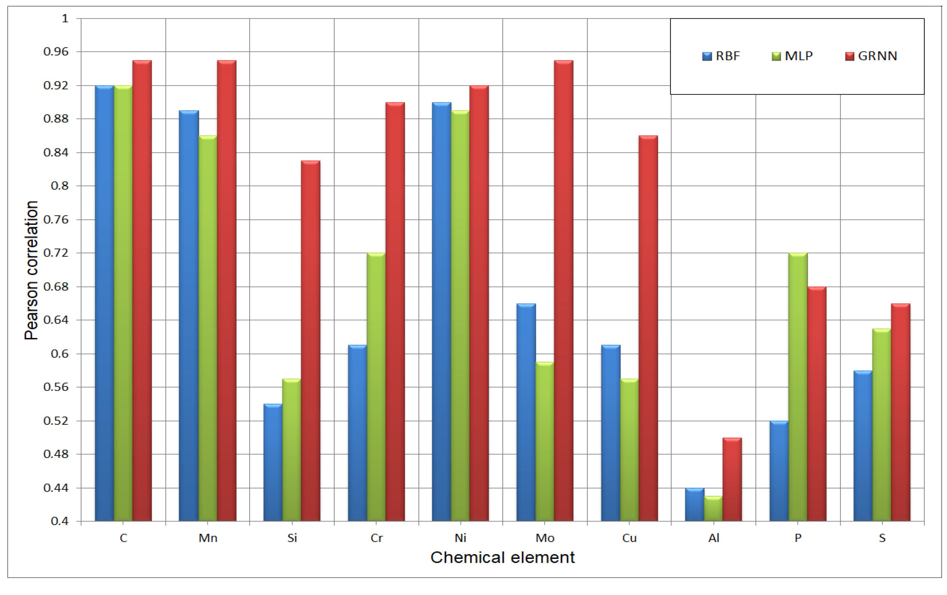
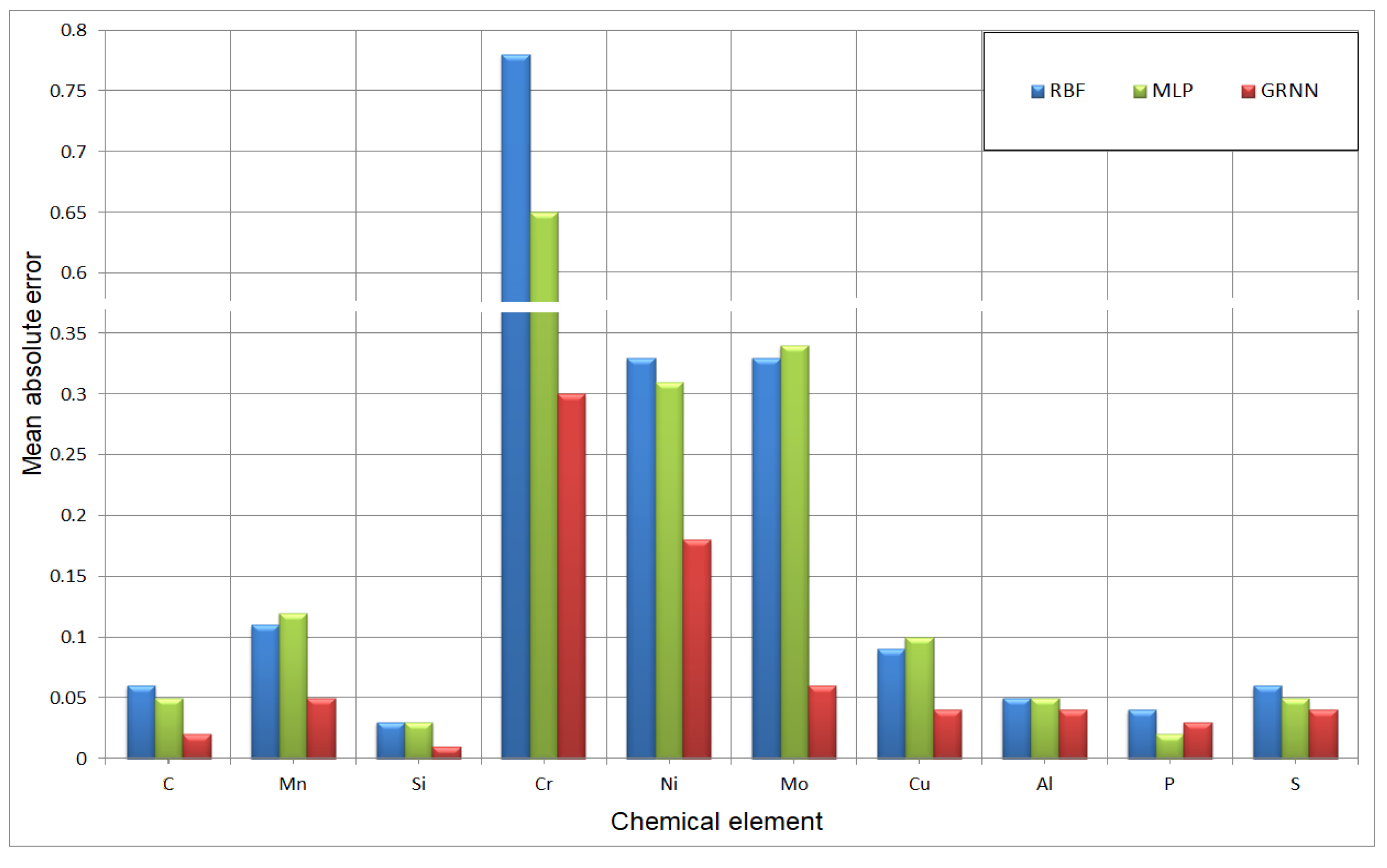
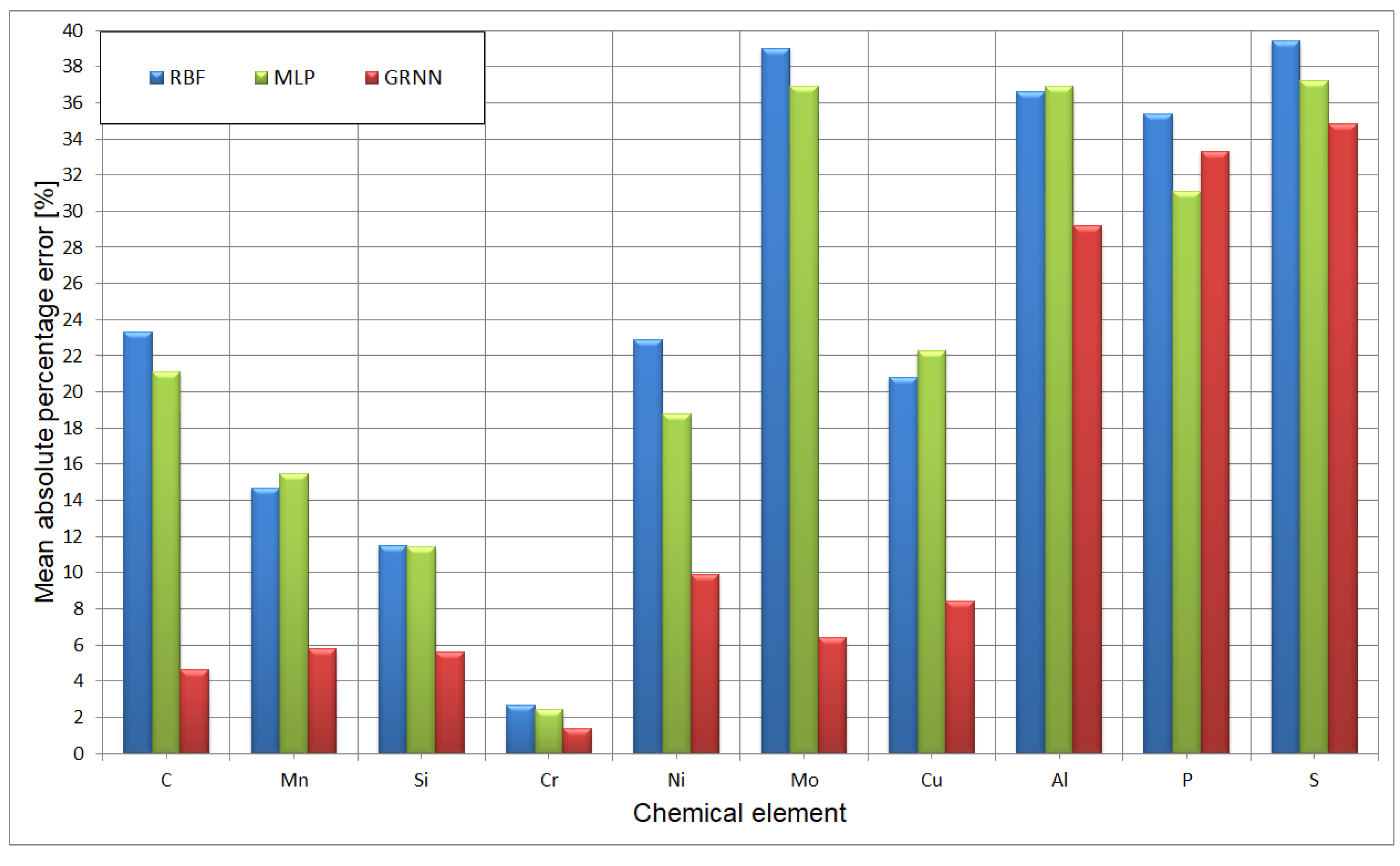
Figure 1 introduces a comparison of the testing set Pearson R correlation of the best artificial neural network of all types, red for RBF, green for MLP and red for GRNN. Greater values are better. Figure 2 introduces a comparison of testing the set mean absolute error of the best artificial neural network of all types; colors are the same, smaller values are better. Figure 3 introduces a comparison of testing the set mean absolute percentage error of the best artificial neural network of all types. Mean absolute percentage error is more readable than mean absolute error because it shows what percentage of the predicted variable is in the prediction error. Again, colors are the same, and smaller values are better.
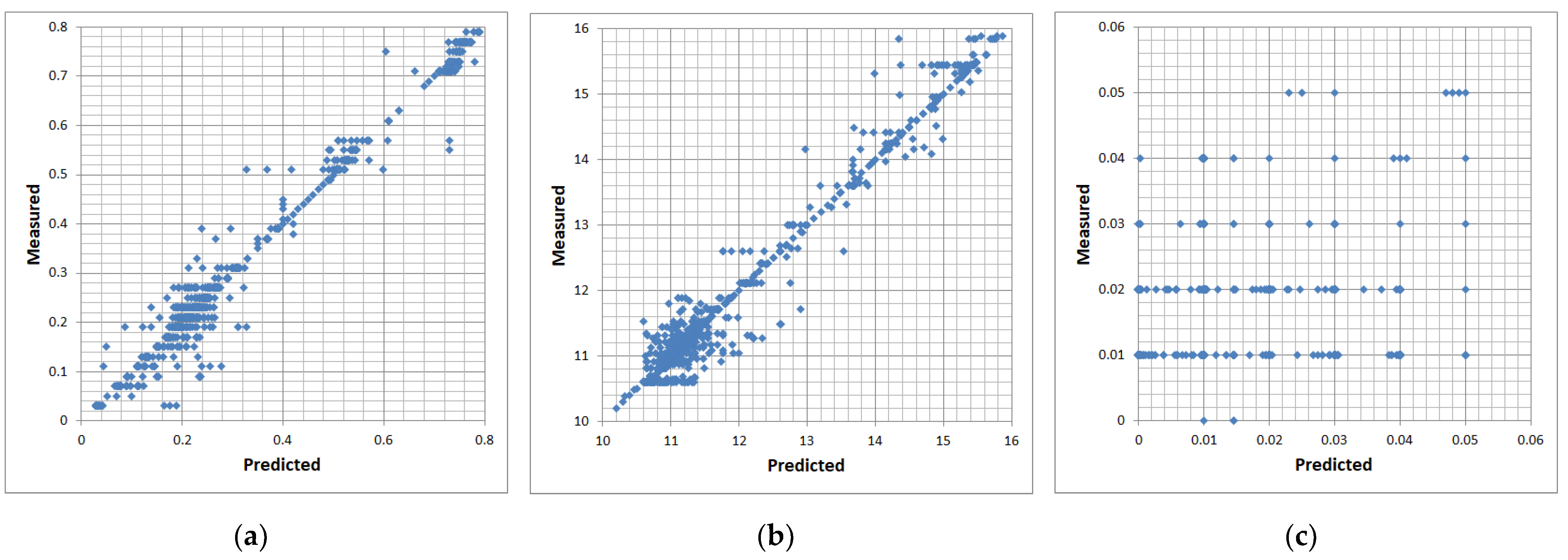
The Pearson R correlation graphs were developed to demonstrate the prediction efficiency in a graphical way. The distinction between the values computed using the artificial neural network and those experimentally tested in the actual laboratory is provided. In all three subsets, the distribution of mechanical property vectors for each of the approximate steel vectors is very similar, confirming the correctness of the learning processes of the networks. Major variations between groups in the distribution of vectors would suggest the probability of errors and, thus, a network of poor quality. Sample graphs of Person R correlation for a testing subset are shown in Figure 4.
4. Discussion
The greatest efficiency in modeling the chemical composition of ferritic stainless steels is shown by general regression neural networks (GRNN). For nine out of ten elements, they have the best regression statistics. The best results were achieved by modeling the concentration of carbon, manganese, chromium, nickel and molybdenum. For these elements, the Pearson correlation exceeded the level of 0.9. Moderately good results were obtained for silicon and copper, where the correlation values are in the range from 0.8 to 0.9. None of the developed networks was able to model the concentrations of aluminum, phosphorus or sulfur.
In the case of carbon, when comparing the Pearson R correlation, it can be seen that all networks were equally good at modeling. The values for the RBF and MLP networks, which are 0.92, differ only slightly from the GRNN networks with a correlation of 0.95. The difference in the mean absolute error is only 0.04 percent of the concentration. The comparisons of the values measured in the laboratory and those obtained computationally, shown in Figure 4a, also show a very good concentration of points. The RBF network rejected one input field which was yield strength (Rp0.2).
In the case of manganese, the GRNN also has the best correlation and the smallest error. The parameters of the RBF and MLP networks are generally lower. Although the correlation is lower by 0.06 in the case of the RBF network and by 0.09 in the case of the MLP network, and the errors of these networks are twice as large as the GRNN network, these values can be considered acceptable. This time, it was the MLP network that rejected the relative elongation A5 as a negligible value in the modeling process.
A similar situation occurred in the case of modeling the nickel concentration. Here also the correlation values between the networks are small and range from 0.89 to 0.92, but the errors are generally larger and amount to 0.18 (9.9%) for GRNN and from 0.31 (18.8%) to 0.33 (22.9%) for other networks. This is related to a higher concentration of this element in the tested steels. All three types of networks can be used for modeling; however, due to the smallest error value, GRNN is recommended.
In the case of chromium and molybdenum, we see a clear advantage of the GRNN network over the other two networks. The difference in correlation is huge, at 0.29 compared to the RBF network. For MLP networks, this difference is not much better. The RBF absolute error difference is almost three times the GRNN error of 0.3 (1.4%). For steels with chromium concentrations greater than ten percent, this is a good result. The variable rejected by the RBF network was tensile strength (Rm). For molybdenum, the difference in absolute error for neural networks is even greater. The RBF error value is almost six times the GRNN error. Further, the correlation of this network of 0.9 is significantly higher than the correlation of the other two networks. The best GRNNs can be successfully used for concentration modeling, the RBF and MLP networks should be rejected as useless. The comparison of the values measured in the laboratory and those obtained computationally for the chromium concentration shown in Figure 4b is as good as for the carbon concentration.
A similar situation as in the case of chromium and molybdenum can be observed in the cases of silicon and copper. There is a clear advantage of the GRNN network over other networks. Although its parameters are not as good as the networks modeling the concentration of elements described above, the result of 0.86 for copper and 0.83 for silicon is quite decent. Additionally, the mean absolute error (mean absolute percentage error) of 0.04 (8.4%) for copper and 0.01 (5.6%) for silicon respectively, is acceptable. In some cases, such as chromium and molybdenum, the parameters of the RBF and MLP networks are so bad that they disqualify both types of networks from use.
Neither type of network has successfully modeled phosphorus, sulfur and aluminum. The network parameters are too bad to be used for modeling. The highest correlation value is only 0.72, and the mean absolute error is too large. In the case of phosphorus, the concentration in the tested steels is 0.05, while the mean absolute error for the MLP network, the network that turned out to be the best, is 0.02. It seems that it is not much, but if we look at the mean absolute percentage error, it is as much as 31.1% of the value. Figure 4c shows how bad it is. For sulfur and aluminum, the network parameters are even worse. In the case of aluminum, the error value is almost 30% of the value, with a Pearson’s R correlation of only 0.5. A large number of rejected input variables, four in the case of the RBF network modeling the sulfur concentration, indicates no relationship between the input and output variables.
5. Conclusions
The concentration of ten chemical elements was modeled on the basis of the mechanical properties of ferritic stainless steels using artificial neural networks with radial basis functions (RBF), multilayer perceptron with one and two hidden layers (MLP) and generalized regression neural network (GRNN).
The best results were achieved for modeling the concentration of carbon, manganese, chromium, nickel and molybdenum. For these elements, the Pearson’s R correlation exceeded the level of 0.9 with a relatively low value of the mean absolute percentage error, which ranges from 1.4% for chromium to 9.9% for nickel. Equally good artificial neural networks, although with slightly lower Pearson’s R correlation values (which were below 0.9 and with mean average percentage errors below 9%) were obtained for silicon and copper.
The regression statistics of these networks indicate that the developed artificial neural networks can be successfully used to predict the chemical composition of ferritic stainless steels.
None of the developed networks were successful in modeling the concentration of aluminum, phosphorus or sulfur. Unfortunately, previous concerns about impurities modeling in ferritic stainless steels have been confirmed. The too low chemical concentration of these elements, and thus too little variability of the values in the training vectors, was the main reason for the failure in properly training any type of artificial neural network and thus in properly modeling these elements.
General regression networks (GRNN) showed the best efficiency in modeling the chemical composition of ferritic stainless steels.
The aim of this paper was an attempt to answer the question of whether, on the basis of the values of the mechanical properties of ferritic stainless steels, it is possible to predict the chemical concentration of carbon and nine other most common alloying elements in these steels. The answer is yes. Since we already know that it is possible, the developed base model may in the future be expanded with new steel grades with different chemical compositions and processed in different ways. This will certainly expand the possibilities of using this model in the industry.
Funding
This research received no external funding.
Institutional Review Board Statement
Not applicable.
Informed Consent Statement
Not applicable.
Data Availability Statement
Data sharing is not possible due to privacy issues.
Conflicts of Interest
The author declares no conflict of interest.
References
- Dobrzański, L.A. Fundamentals of Materials Science and Metallurgy; WNT: Warszawa, Poland, 2002. [Google Scholar]
- Dobrzański, L.A. Metal Engineering Materials; WNT: Warszawa, Poland, 2004. (In Polish) [Google Scholar]
- Dobrzański, L.A.; Honysz, R. Virtual examinations of alloying elements influence on alloy structural steels mechanical properties. J. Mach. Eng. 2011, 49, 102–119. [Google Scholar]
- Musztyfaga-Staszuk, M.; Honysz, R. Application of artificial neural networks in modeling of manufactured front metallization contact resistance for silicon solar cells. Arch. Metall. Mater. 2015, 60, 673–678. [Google Scholar] [CrossRef] [Green Version]
- Dobrzański, L.A.; Honysz, R. Computer modelling system of the chemical composition and treatment parameters influence on mechanical properties of structural steels. J. Achiev. Mater Manuf. Eng. 2009, 35, 138–145. [Google Scholar]
- Marciniak, A.; Korbicz, J. Data preparation and planning of the experiment. In Artificial Neural Networks in Biomedical Engineering; Tadeusiewicz, R., Korbicz, J., Rutkowski, L., Duch, W., Eds.; EXIT Academic Publishing House: Warsaw, Poland, 2013; Volume 9. [Google Scholar]
- Sitek, W. Metodologia Projektowania Stali Szybkotnących z Wykorzystaniem Narzędzi Sztucznej Inteligencji; International Ocsco World Press: Gliwice, Poland, 2010. (In Polish) [Google Scholar]
- Trzaska, J. Metodologia Prognozowania Anizotermicznych Krzywych Przemian Fazowych Stali Konstrukcyjnych i Maszynowych; Silesian University of Technology Publishing House: Gliwice, Poland, 2017. (In Polish) [Google Scholar]
- Honysz, R.; Dobrzański, L.A. Virtual laboratory methodology in scientific researches and education. J. Achiev. Mater Manuf. Eng. 2017, 2, 76–84. [Google Scholar] [CrossRef]
- Information about Steel for Metallographer. Available online: http://metallograf.de/start-eng.htm (accessed on 20 February 2021).
- MatWeb. Your Source for Materials Information. Available online: http://matweb.com (accessed on 20 February 2021).
- Feng, W.; Yang, S. Thermomechanical processing optimization for 304 austenitic stainless steel using artificial neural network and genetic algorithm. J. Appl. Phys. 2016, 122, 1–10. [Google Scholar] [CrossRef]
- Kim, Y.-H.; Yarlagadda, P. The Training Method of General Regression Neural Network for GDOP Approximation. Appl. Mech. Mater. 2013, 278–280, 1265–1270. [Google Scholar] [CrossRef]
- Mandal, S.; Sivaprasad, P.V.; Venugopal, S. Capability of a Feed-Forward Artificial Neural Network to Predict the Constitutive Flow Behavior of As Cast 304 Stainless Steel Under Hot Deformation. J. Eng. Mater. Technol. 2007, 2, 242–247. [Google Scholar] [CrossRef]
- Kapoor, R.; Pal, D.; Chakravartty, J.K. Use of artificial neural networks to predict the deformation behavior of Zr–2.5Nb–0.5Cu. J. Mater. Process. Technol. 2005, 169, 199–205. [Google Scholar] [CrossRef]
- Jovic, S.; Lazarevic, M.; Sarkocevic, Z.; Lazarevic, D. Prediction of Laser Formed Shaped Surface Characteristics Using Computational Intelligence Techniques. Laser. Eng. 2018, 40, 239–251. [Google Scholar]
- Karkalos, N.E.; Markopoulos, A.P. Determination of Johnson-Cook material model parameters by an optimization approach using the fireworks algorithm. Proc. Manuf. 2018, 22, 107–113. [Google Scholar] [CrossRef]
- Trzaska, J. Neural networks model for prediction of the hardness of steels cooled from the austenitizing temperature. Arch. Mater. Sci. Eng. 2016, 82, 62–69. [Google Scholar]
- Masters, T.; Land, W. New training algorithm for the general regression neural network. In Proceedings of the IEEE International Conference on Systems, Man and Cybernetics. Computational Cybernetics and Simulation, Orlando, FL, USA, 12–15 October 1997; Volume 3. [Google Scholar] [CrossRef]
- Jimenez-Come, M.J.; Munoz, E.; Garcia, R.; Matres, V.; Martin, M.L.; Trujillo, F.; Turiase, I. Pitting corrosion behaviour of austenitic stainless steel using artificial intelligence techniques. J. Appl. Logic. 2012, 10, 291–297. [Google Scholar] [CrossRef] [Green Version]
- Shen, C.; Wang, C.; Wei, X.; Li, Y.; van der Zwaag, S.; Xua, W. Physical metallurgy-guided machine learning and artificial intelligent design of ultrahigh-strength stainless steel. Acta Mater. 2019, 179, 201–214. [Google Scholar] [CrossRef]
- Adamczyk, J. Metallurgy Theoretical Part 1. The Structure of Metals and Alloys; Silesian University of Technology: Gliwice, Poland, 1999. (In Polish) [Google Scholar]
- Adamczyk, J. Metallurgy Theoretical Part 2. Plastic Deformation, Strengthening and Cracking; Silesian University of Technology: Gliwice, Poland, 2002. (In Polish) [Google Scholar]
- Dobrzański, L.A. Engineering Materials and Materials Design. Fundamentals of Materials Science and Physical Metallurgy; WNT: Warsaw, Poland; Gliwice, Poland, 2006. (In Polish) [Google Scholar]
- Totten, G.E. Steel Heat Treatment: Metallurgy and Technologies; CRC Press: New York, NY, USA, 2006. [Google Scholar]
- PN-EN 10002-1: 2002. Available online: http://www.pkn.pl/ (accessed on 20 February 2021).
- PN-EN ISO 6506-1: 2002. Available online: http://www.pkn.pl/ (accessed on 20 February 2021).
- Sitek, W. Employment of rough data for modelling of materials properties. Achiev. Mater. Manuf. Eng. 2007, 21, 65–68. [Google Scholar]
- Honysz, R. Optimization of Ferrite Stainless Steel Mechanical Properties Prediction with artificial intelligence algorithms. Arch. Metall. Mater. 2020, 65, 749–753. [Google Scholar] [CrossRef]
- Michalewicz, Z. Genetic Algorithms + Data Structures = Evolutionary Programs; WNT: Warsaw, Poland, 2003. [Google Scholar]
- Sammut, C.; Webb, G.I. (Eds.) Encyclopedia of Machine Learning and Data Mining; Springer Science & Business Media: New York, NY, USA, 2017. [Google Scholar]
- Rutkowski, L. Methods and Techniques of Artificial Intelligence; PWN: Warszawa, Poland, 2006. [Google Scholar]
- Tadeusiewicz, R. Artificial Neural Networks; Academic Publishing House: Warsaw, Poland, 2001. [Google Scholar]
- Tadeusiewicz, R.; Szaleniec, M. Leksykon Sieci Neuronowych; Wydawnictwo Fundacji “Projekt Nauka”: Wrocław, Poland, 2015. [Google Scholar]
- Specht, D.F. A general regression neural network. IEEE Trans. Neural Netw. Learn. Syst. 2002, 2, 568–576. [Google Scholar] [CrossRef] [PubMed] [Green Version]
- Strumiłło, P.; Kamiński, W. Radial basis function neural networks: Theory and applications. In Neural Networks and Soft Computing; Rutkowski, L., Kacprzyk, J., Eds.; Physica: Heidelberg, Germany, 2003; Volume 19. [Google Scholar] [CrossRef]
- Aitkin, M.; Foxall, R. Statistical modelling of artificial neural networks using the multi-layer perceptron. Stat. Comput. 2003, 13, 227–239. [Google Scholar] [CrossRef]
- Dobrzański, L.A.; Honysz, R. Artificial intelligence and virtual environment application for materials design methodology. Arch. Mater. Sci. Eng. 2010, 45, 69–94. [Google Scholar]
- Ossowski, S. Sieci Neuronowe w Ujęciu Algorytmicznym; WNT: Warszawa, Poland, 1996. (In Polish) [Google Scholar]
- Patterson, D.W. Artificial Neural Networks—Theory and Applications; Prentice-Hall: Englewood Cliffs, NJ, USA, 1998. [Google Scholar]
- Statology. Statistic Simplified. Available online: https://www.statology.org/ (accessed on 20 February 2021).
- StatSoft Europe. Available online: http://www.statsoft.pl/ (accessed on 20 February 2021).
Figure 1.
Comparison of Pearson correlation for the best achieved artificial neural networks (testing set), built for examinate steels.
Figure 1.
Comparison of Pearson correlation for the best achieved artificial neural networks (testing set), built for examinate steels.

Figure 2.
Comparison of mean absolute error for the best achieved artificial neural networks (testing set), build for examinate steels.
Figure 2.
Comparison of mean absolute error for the best achieved artificial neural networks (testing set), build for examinate steels.

Figure 3.
Comparison of mean absolute percentage error for the best achieved artificial neural networks (testing set), build for examinate steels.
Figure 3.
Comparison of mean absolute percentage error for the best achieved artificial neural networks (testing set), build for examinate steels.

Figure 4.
Examples of comparative graphs for (a) carbon concentration, (b) chromium concentration and (c) phosphorus concentration, calculated with use of the artificial neural networks and determined experimentally.
Figure 4.
Examples of comparative graphs for (a) carbon concentration, (b) chromium concentration and (c) phosphorus concentration, calculated with use of the artificial neural networks and determined experimentally.


Table 1.
The range of selected input variable values.
| Range | Mechanical Properties | |||||
|---|---|---|---|---|---|---|
| Rp0.2 (MPa) | Rm (MPa) | A (%) | Z (%) | KCU2 (J/mm2) | HB | |
| minimum | 208 | 369 | 3 | 15 | 14 | 111 |
| maximum | 920 | 970 | 65 | 78 | 348 | 331 |
Table 2.
Architecture and regression parameters of developed artificial neural networks (testing set).
Table 2.
Architecture and regression parameters of developed artificial neural networks (testing set).
| Chemical Element | RBF Network | MLP Network | GRNN Network | |||||||||
|---|---|---|---|---|---|---|---|---|---|---|---|---|
| AR | MAE | MAPE | R | AR | MAE | MAPE | R | AR | MAE | MAPE | R | |
| C | 5-33-1 | 0.50 | 23.3% | 0.92 | 6-7-1 | 0.57 | 21.1% | 0.92 | 6-1636-2-1 | 0.01 | 4.6% | 0.95 |
| Mn | 6-54-1 | 0.11 | 14.7% | 0.89 | 5-15-5-1 | 0.12 | 15.5% | 0.86 | 6-1636-2-1 | 0.05 | 5.8% | 0.95 |
| Si | 5-24-1 | 0.03 | 11.5% | 0.54 | 6-13-1 | 0.03 | 11.4% | 0.57 | 6-1636-2-1 | 0.01 | 5.6% | 0.83 |
| Cr | 5-12-1 | 0.78 | 2.7% | 0.61 | 6-15-1 | 0.65 | 2.4% | 0.72 | 6-1636-2-1 | 0.3 | 1.4% | 0.90 |
| Ni | 6-30-1 | 0.33 | 22.9% | 0.90 | 6-10-1 | 0.31 | 18.8% | 0.89 | 6-1636-2-1 | 0.18 | 9.9% | 0.92 |
| Mo | 6-28-1 | 0.33 | 39.0% | 0.66 | 6-9-1 | 0.34 | 36.9% | 0.59 | 6-1636-2-1 | 0.06 | 6.4% | 0.95 |
| Cu | 6-57-1 | 0.09 | 20.8% | 0.61 | 6-23-2-1 | 0.10 | 22.3% | 0.57 | 6-1636-2-1 | 0.04 | 8.4% | 0.86 |
| Al | 3-18-1 | 0.05 | 36.6% | 0.44 | 3-2-1 | 0.05 | 36.9% | 0.43 | 6-1636-2-1 | 0.04 | 29.2% | 0.50 |
| P | 5-9-1 | 0.04 | 35.4% | 0.52 | 6-15-1 | 0.02 | 31.1% | 0.72 | 5-1636-2-1 | 0.03 | 33.3% | 0.68 |
| S | 2-10-1 | 0.06 | 39.4% | 0.58 | 5-2-1 | 0.05 | 37.2% | 0.63 | 4-1636-2-1 | 0.04 | 34.8% | 0.66 |
Where: AR—neural network architecture; MAE—mean absolute error; MAPE—mean absolute percentage error; R—Pearson R correlation.
Publisher’s Note: MDPI stays neutral with regard to jurisdictional claims in published maps and institutional affiliations. |
© 2021 by the author. Licensee MDPI, Basel, Switzerland. This article is an open access article distributed under the terms and conditions of the Creative Commons Attribution (CC BY) license (https://creativecommons.org/licenses/by/4.0/).
Share and Cite
MDPI and ACS Style
Honysz, R. Modeling the Chemical Composition of Ferritic Stainless Steels with the Use of Artificial Neural Networks. Metals 2021, 11, 724. https://doi.org/10.3390/met11050724
AMA Style
Honysz R. Modeling the Chemical Composition of Ferritic Stainless Steels with the Use of Artificial Neural Networks. Metals. 2021; 11(5):724. https://doi.org/10.3390/met11050724
Chicago/Turabian StyleHonysz, Rafał. 2021. "Modeling the Chemical Composition of Ferritic Stainless Steels with the Use of Artificial Neural Networks" Metals 11, no. 5: 724. https://doi.org/10.3390/met11050724
Note that from the first issue of 2016, this journal uses article numbers instead of page numbers. See further details here.