Prediction of Mechanical Properties for High Strength Low Alloyed Steels in a Commercial Hot Dip Galvanizing Line without Soaking Section

Abstract

The classical thermal cycle in a Hot Dip Galvanizing (HDG) line has four steps: heating, soaking, cooling, and aging. The furnace of an ArcelorMittal HDG line was revamped to increase its heating capacity. This new configuration without the soaking step led to the redefinition of the thermal cycles for all the steel grades, especially for High Strength Low Alloyed (HSLA) steels, where it was necessary to define a new control parameter based on time and temperature. This paper presents the work done to improve the control of the mechanical properties of HSLA steels in the HDG line. Four different types of numerical models (linear and polynomial regressions, artificial neural networks, and Multivariate Adaptive Regression Splines), are applied to predict the yield strength and the tensile strength of individual coils. It is concluded that the introduction of the time–temperature parameter improves the accuracy of the predictions over 10% in most of the cases. An additional improvement is obtained with the use of the process values corresponding to the sampling area instead of the coil average ones. The use of these models makes it possible, if necessary, to adjust individually the presets of the coils before processing them in the galvanizing line and reduce the scattering of the mechanical properties.

1. Introduction

The mechanical properties of a coated coil are obtained after passing the material along several stages. The initial one is in the Steel Mill (SM), where the chemical composition of the liquid steel is adjusted and then solidified in the continuous caster. The next step is the Hot Strip Mill (HSM), where the slab, a steel ingot of rectangular shape, is rolled and transformed into a coil. In the Pickling Line (PL), the scale formed in the surface of the coil during the hot rolling is removed by immersion in tanks with acid. The pickled coil is then rolled again in the Cold Rolling Mill (CRM) to adjust the thickness to the target one. The last stage is the coating process; it is carried out in the Hot Dip Galvanizing line (HDG), where before the coating process, it is necessary to anneal the steel to recover the microstructure and grain size. These are key factors in the properties of the coil, and which were affected by the rolling process in the Cold Rolling Mill.

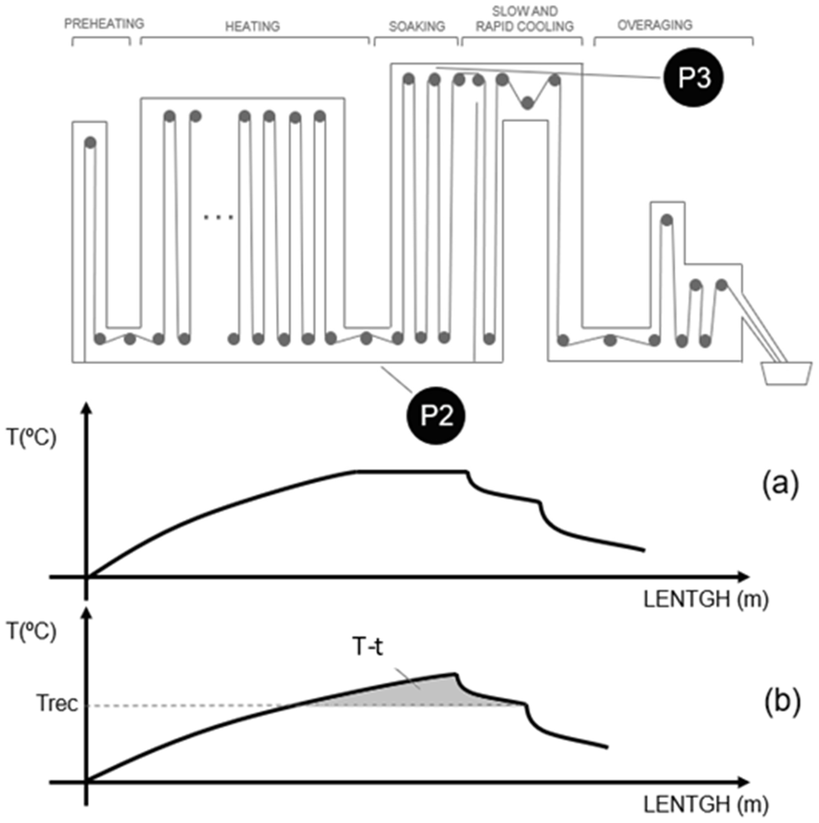
Figure 1 shows the layout of the annealing furnace and the traditional thermal cycle (Figure 1a), where the peak temperature is achieved at point P2. The revamping of the annealing furnace of a galvanizing line meant the redesign of the thermal cycles for the product mix produced. Figure 1b shows the new cycle without soaking, where the peak temperature is achieved at point P3. In the case of the High Strength Low Alloyed (HSLA) steels, it was necessary to introduce a new control parameter to ensure the mechanical properties, called the time–temperature [1], and its value corresponds to the area comprised in between the thermal profile and the recrystallization temperature, T_rec with a value of 725 °C, as is shown in Figure 1c.

The definition of the cycles also changed from a classical cycle with a target temperature plus-minus a given margin. Whatever the speed, it is passed to a speed given by a combination of target temperature and strip thickness [1]. For example, a classical cycle can point to 815 ± 15 °C, with an annealing time between 2 to 5 min, depending on the strip thickness. The speed range, and so the annealing time, is calculated with the following equations:

$$S_{min,i}={\displaystyle \sum }_1^3{a}_{j}t{h}^{3-j}{T}_i^2+{\displaystyle \sum }_1^3{b}_{j}t{h}^{3-j}{T}_i+{\displaystyle \sum }_1^3{c}_{j}t{h}^{3-j}$$

(1)

$$S_{max,i}={\displaystyle \sum }_1^3{d}_{j}t{h}^{3-j}{T}_i^2+{\displaystyle \sum }_1^3{e}_{j}t{h}^{3-j}{T}_i+{\displaystyle \sum }_1^3{f}_{j}t{h}^{3-j}$$

(2)

Where th is the thickness of the strip, S_min,i and S_max,i are the minimum and maximum speeds allowed for a target temperature T_i, and the coefficients a_j to c_j and d_j to f_j are calculated from the upper and lower limits of the time–temperature parameter, respectively. Therefore, for the same steel grade, the target temperature and annealing time depends on the strip thickness.

This parameter is useful for the online assessment of the coil, but the limits are calculated for the whole steel grade, which includes all the coils with the same chemical composition without considering the parameters used in upstream processes. So, if the more accurate prediction of the mechanical properties of a specific coil is desired, further development is needed.

It is possible to develop a metallurgical model based on laboratory tests, linking the mechanical properties with the microstructure obtained for a given composition and manufacturing parameters of the sample [2], but it is hard to reproduce the complete process (hot rolling, cold rolling, and annealing) in the lab. Working with individual industrial samples adds uncertainty about the exact values of the process parameters because of dimensional changes produced by the processes themselves or the reparation of the coils, which implies removing parts of the coils between the mills. This makes it difficult, in some cases, to match the sampling area with the corresponding value of the process parameter along with all the mills.

When the effect of several different processes is to be studied, the use of data-driven models seems to be a good option. The correct selection of the variables and the quality of the data will impact on the reliability of these models. In this study, the results of the prediction of the yield strength and ultimate tensile strength of the coils using different types of data models are compared. The modeling of the effect of process parameters on the mechanical properties using neural networks to reduce the number of lab tests has been addressed previously [3]. Other researches have combined process parameters and initial microstructure to analyze the effect of each one on the sensitivity of the model and for modeling the influence of alloying elements on the final properties [4,5].

Studies about the effect of modifying the architecture of an artificial neural network to reduce the number of epochs required to reach the targeted error and comparisons of the performance of neural networks versus the Multivariate Adaptive Regression Splines (MARS) can also be found [6,7]. There are also examples of the combination of neural networks and computer simulations with computational fluid dynamics software to predict the mechanical properties and microstructure [8], and recently neural networks with genetic algorithms for designing dual-phase steels with the improved performance [9]. Combining physical models with neural networks has proven to be an effective method for improving the accuracy of the prediction of hot deformation behavior [10].

In light of previous research, the trend is to combine different tools and build more complex models to improve the accuracy of the predictions. In some cases, this may not be necessary if additional process parameters can be defined. The aim of this work is to evaluate the improvement in the predictions of the mechanical properties of the HSLA steels in an annealing furnace without the soaking phase when including the time–temperature parameter in the different studied models.

The final objective is to improve the prediction of the yield strength (YS) and ultimate tensile strength (UTS) of individual coils using data-driven models. The final values of the tensile strength and ultimate yield strength of the coil at the exit of a galvanizing line depend on the chemical composition of the coil and the process parameters used in the line and in the upstream mills [11].

The rest of the paper is organized as follows; first the applied methodology and the selection of parameters are explained. Then, the composition of the datasets used and the four types of models are presented. Finally, the results of the predictions for different models are analyzed, and the practical application of this study is explained.

2. Materials and Methods

This work was addressed using the Cross-Industry Standard Process for Data Mining (CRISP-DM) methodology [12], which is used for carrying out data mining projects independent of both the industry sector and the technology used. This methodology is based in six phases: the initial stages of this method imply the business understanding, the data understanding, and the data preparation. The next phases include the modeling itself, the evaluation of the results obtained, and the deployment of the model. In the present study, the results of four different models will be compared: linear regression, polynomial regression, artificial neural networks, and MARS.

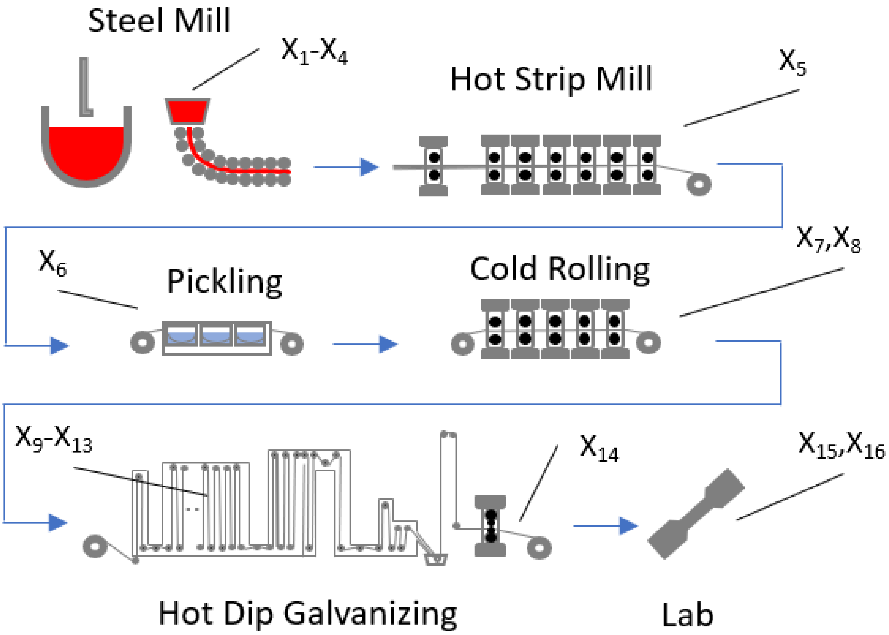
Fifty-two process parameters from Steel Mill, Hot Strip Mill, Pickling Line, Cold Rolling Mill, and Hot Dip Galvanizing line were collected and organized from the different databases. These parameters included the chemical composition of the coils and the main process parameters of each installation (processing speeds, temperatures, forces, tensions, reduction rate). Figure 2 shows the different stages of the process and where the variables used in the models are obtained. The data correspond to the period 2018–2019. The data were filtered to select the coils belonging to HSLA260 and HSLA300 grades and all registers with zeros in the YS, UTS, or any of the process parameters were removed to obtain the final datasets.

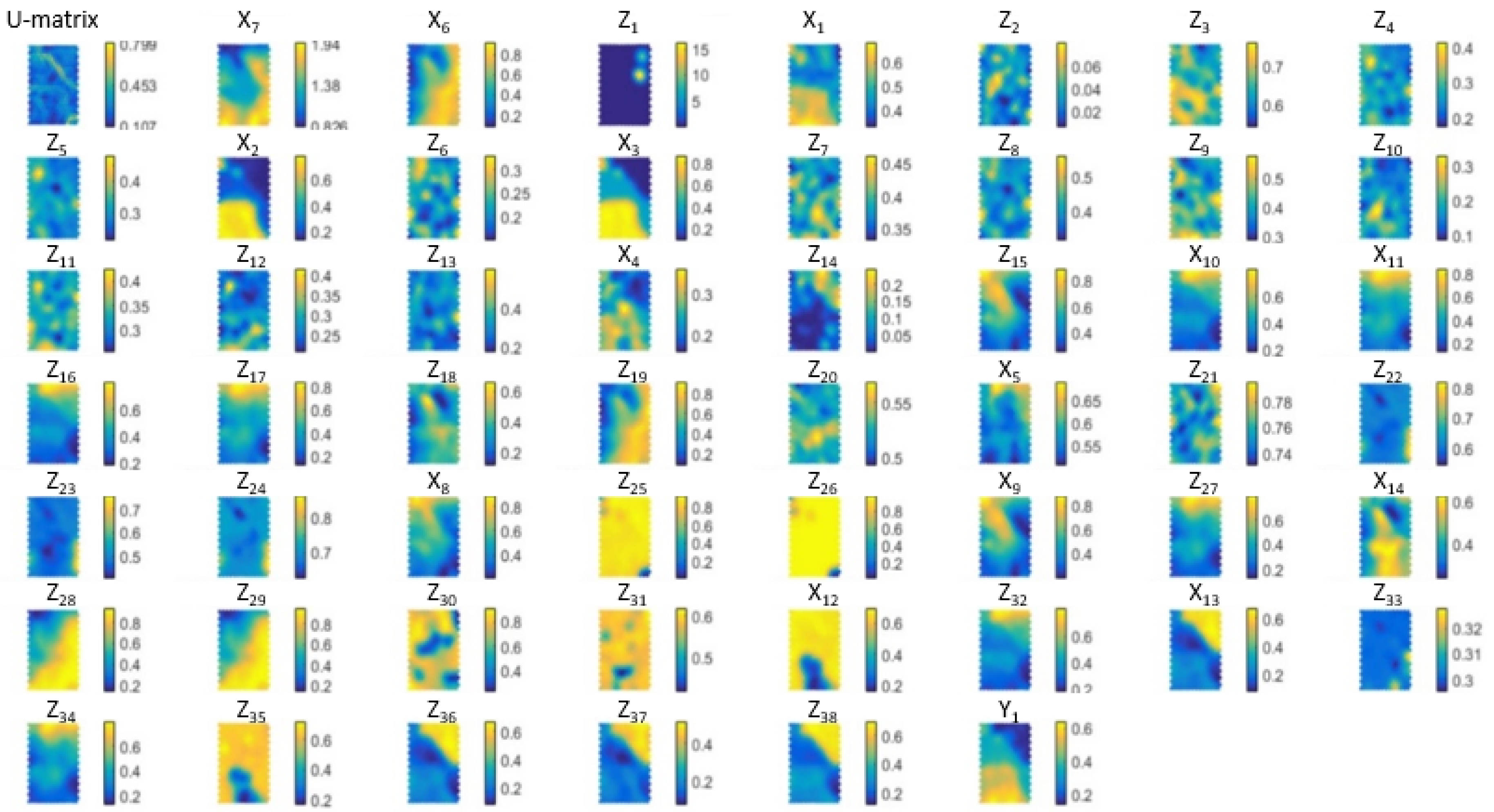
The Self-Organized Maps (SOM) technique [13] was used to reduce the initial number of input variables, comparing the similarities of the resulting maps for each variable with the yield strength map because the observed scattering in its measurements was higher than the scattering on the measurements of the ultimate tensile strength [1].

Figure 3 shows the output of the SOM analysis for the initial set of values. The SOM is a type of neural network which creates a two-dimensional representation of a multidimensional space, where more neurons point to regions with high training sample concentration and fewer where the samples are scarce. The discarded variables are shown in

Table 1. List of variables discarded by means of the SOM analysis.

Name	Description	Type of Variable	Origin
Z1	Boron content	Chemical	SM
Z2	Calcium content	Chemical	SM
Z3	Cobalt content	Chemical	SM
Z4	Chrome content	Chemical	SM
Z5	Copper content	Chemical	SM
Z6	Molybdenum content	Chemical	SM
Z7	Nitrogen content	Chemical	SM
Z8	Nickel content	Chemical	SM
Z9	Phosphorus content	Chemical	SM
Z10	Lead content	Chemical	SM
Z11	Sulfur content	Chemical	SM
Z12	Silicon content	Chemical	SM
Z13	Tin content	Chemical	SM
Z14	Vanadium content	Chemical	SM
Z15	Maximum speed	Process Parameter	HDG
Z16	Coiling tension	Process Parameter	CRM
Z17	Intermediate cooling temperature	Process Parameter	HSM
Z18	Deviation of skin pass force	Process Parameter	HDG
Z19	Width at hot rolling mill	Process Parameter	HSM
Z20	Cooling exit temperature	Process Parameter	HSM
Z21	Heating temperature	Process Parameter	HSM
Z22	Average elongation at skin pass	Process Parameter	HDG
Z23	Maximum elongation at skin pas	Process Parameter	HDG
Z24	Minimum elongation at skin pass	Process Parameter	HDG
Z25	Rolling entry temperature	Process Parameter	HSM
Z26	Deviation of cooling exit temperature	Process Parameter	HSM
Z27	Deviation at P3	Process Parameter	HDG
Z28	Skin pass entry tension	Process Parameter	HDG
Z29	Skin pass exit tension	Process Parameter	HDG
Z30	Entry temperature at heating	Process Parameter	HDG
Z31	Temperature at slow cooling	Process Parameter	HDG
Z32	Deviation at P2	Process Parameter	HDG
Z33	In/Out skin tension difference	Process Parameter	HDG
Z34	% of austenite calculated	Process Parameter	HDG
Z35	Cooling ratio	Process Parameter	HDG
Z36	Deviation T-t	Process Parameter	HDG
Z37	Maximum T-t	Process Parameter	HDG
Z38	Minimum T-t	Process Parameter	HDG

and the final variables used for building the models are in

Table 2. List of variables used in the models.

Name	Description	Type of Variable	Origin	Model
X1	Carbon content	Chemical	SM	Input
X2	Manganese content	Chemical	SM	Input
X3	Niobium content	Chemical	SM	Input
X4	Titanium content	Chemical	SM	Input
X5	Coiling temperature	Process Parameter	HSM	Input
X6	Coil width	Dimensional	PL	Input
X7	Coil thickness	Dimensional	CRM	Input
X8	Cold rolling reduction	Process Parameter	CRM	Input
X9	Line speed	Process Parameter	HDG	Input
X10	Intermediate temperature	Process Parameter	HDG	Input
X11	Coil target temperature	Process Parameter	HDG	Input
X12	End cooling temperature	Process Parameter	HDG	Input
X13	Time–temperature parameter	Process Parameter	HDG	Input
X14	Skin pass force	Process Parameter	HDG	Input
Y1	Yield strength	Measurement	Lab	Output
Y2	Ultimate tensile strength	Measurement	Lab	Output

; a reduction in the input parameters from 52 to 14 was achieved. This selection was based on the similarity of the map of each parameter with the map of the yield strength (Y₁ in Figure 3). The U-matrix represents the distance between the neurons to assess the topological correctness of the SOM and to identify clusters [14].

Most of the variables of the list have a clear relation with the mechanical properties: the chemical composition plays obviously an important role as the formation of stable carbides enhances the strength [15], and it has also been reported that the presence of titanium can interfere with the precipitation of vanadium nitrides and carbonitrides [16,17]. The effect of decreasing the coiling temperature in Nb-alloyed HSLA was pointed is some papers [18,19]. It is also in literature that the higher the cold reduction of the material before annealing, the lower the recrystallization temperature [20]. The effect on mechanical properties of skin-pass parameters [21], or annealing time and temperature [22,23,24] were also proved.

Including width and thickness parameters is interesting for classification purposes, and additional process parameters from the HDG line as speed or end cooling temperature were also included because in the SOM there are some ranges of them (corresponding to areas of the map of these parameters), where similarity with the map of the yield strength can be established.

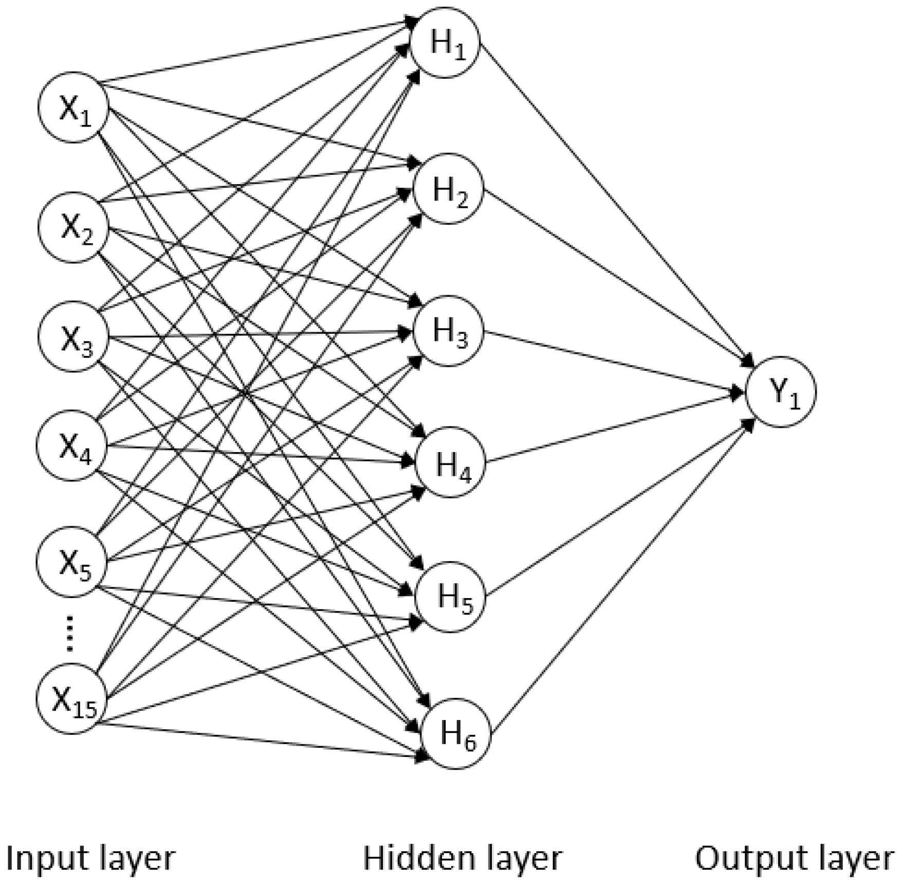
The next step of the methodology is modeling. Four different types of modeling techniques are used for the predictors: multiple linear regression, multiple polynomial regression, artificial neural network (ANN), and Multivariate Adaptive Regression Splines (MARS). The multiple linear regression has advantages such as its ease and speed of computation, but on the other hand, they make a strong assumption about linearity. Multiple polynomial regressions are an extension of linear regressions to capture nonlinear relationships by adding additional predictors obtained by raising each of the original predictors to a power. An artificial neural network ANN contains layers of interconnected nodes, where each node or perceptron is similar to a multiple linear regression [25]. The perceptron feeds the signal produced by a multiple linear regression into an activation function that may be nonlinear. The Multivariate Adaptive Regression Splines (MARS) provide a convenient approach to capture the nonlinearity aspect of polynomial regression by assessing cut points (knots) similar to step functions [26]. The procedure assesses each data point for each predictor as a knot and creates a linear regression model with the candidate features.

In the present study, the four types of models were applied to two different families of HSLA steels with the characteristics shown in

Table 3. Composition (% in mass) and mechanical properties of steel grades studied.

Grade	C Max	Mn Max	Si Max	YS (MPa)	UTS (MPa)
HSLA 260	0.080	0.50	0.04	260–320	350–410
HSLA 300	0.080	0.60	0.04	300–360	390–450

.

The raw data correspond to the period from July 2018 to July 2019. The initial dataset is composed of the coils produced using the denomination HSLA 260 and HSLA 300. Registers of the database with errors or zeros in any of the parameters were removed.

Table 4. Composition of the datasets used in the study.

Parameters	Dataset Composition
	1A	1B	2A	2B
X1, X2, X3, X4, X5, X6, X7, X8	Average	Average	Average	Average
X9, X10, X11, X12, X14	Average	Average	Tail	Tail
X13	No	Yes	No	Yes

shows the composition of the dataset used: 1A is composed of the average values of the input parameters of the coils; the dataset 2A changes the average values in the HDG by those associated with the tail of the coil (sampling area). In both datasets, a B version was built by adding the value of the time–temperature parameter to evaluate the improvement in the results. The number of samples used is 725 in the case of HSLA 260 and 1176 in the case of HSLA 300.

2.1. Multiple Linear Regression

Multiple linear regression is a statistical technique that uses several explanatory variables to predict the outcome of a response variable. This method assumes a linear relationship between the dependent variables and the independent variables, and that the independent variables are not too highly correlated with each other.

In this case, the predictor was developed with the open software KNIME Analytics Platform v4.1 (KNIME AG. Zurich, Switzerland) [27], and the diagram block is shown in Figure 4. For the validation, the X-Partitioner block is used, which divides the total set of samples in ten groups, taking eight for creating the model and two for testing. This process is repeated ten times, taking the groups randomly to avoid the overestimation of the error done when fixed learning and test groups are taken.

The regressions have the following expression:

$$Y_1={\displaystyle \sum }_1^{14}\left(A_i{X}_i\right)+CL{R}_{YS}$$

(3)

$$Y_2={\displaystyle \sum }_1^{14}\left(B_i{X}_i\right)+CL{R}_{UTS}$$

(4)

where Y₁ is the yield strength, Y₂ is the ultimate tensile strength, A_i and B_i are the coefficients calculated, X_i the independent variables, and CLR_YS and CLR_UTS constants.

2.2. Multiple Polynomial Regression

The predictor was also developed with the open software KNIME, and the block diagram is the same as in Figure 4, only changing the regression block. The partitioner block was also configured with ten cross-validations and random sampling, as in the previous case. The absolute mean error (MAE) was the indicator taken for the selection of the regression degree, being n the number of samples available for each steel grade.

$$MA{E}_{YS}=\frac{{{\displaystyle \sum }}_{i=1}^n\left|Y_1-X_{15}\right|}{n};MA{E}_{UTS}=\frac{{{\displaystyle \sum }}_{i=1}^n\left|Y_2-X_{16}\right|}{n}$$

(5)

The regression was set as the 4th degree because a higher degree made the error in the YS raise, as is shown in

Table 5. Study of the error (MPa) with different polynomial degrees.

Steel Grade	YS			UTS
	Poly. Grade			Poly. Grade
	3	4	5	3	4	5
HSLA 260	7.25	7.3	14.15	5.72	5.22	4.88
HSLA 300	10.20	9.83	10.12	7.66	7.15	7.02

.

The polynomial regression has the following expression:

$$Y_1={\displaystyle \sum }_1^{14}\left(D_{4i}{X}_i^4+D_{3i}{X}_i^3+D_{2i}{X}_i^2+D_{1i}{X}_i\right)+CP{R}_{YS}$$

(6)

$$Y_2={\displaystyle \sum }_1^{14}\left(E_{4i}{X}_i^4+E_{3i}{X}_i^3+E_{2i}{X}_i^2+E_{1i}{X}_i\right)+CP{R}_{UTS}$$

(7)

where D_xi and E_xi are the calculated coefficients, and CPR_YS and CPR_UTS are constants.

2.3. Artificial Neural Network

A multilayer perceptron (MLP) is a group of perceptrons, organized in several layers, that can accurately answer complex questions. Each perceptron of the first layer (Figure 5 on the left) sends signals to all the perceptrons of the second layer, and so on. An MLP contains an input layer, at least one hidden layer, and an output layer.

The neural network was implemented with the software KNIME. It has one layer because the tests with more layers did not improve the results. The number of perceptrons was also tested, with the results being quite homogeneous but with slightly lower errors when using six neurons, as shown in

Table 6. Study of the error (MPa) with a different number of perceptrons.

Steel Grade	Dataset 1A			Dataset 1B
	Number of Neurons			Number of Neurons
	4	6	8	4	6	8
HSLA 260	6.11	6.07	6.24	6.31	6.17	6.28
HSLA 300	7.50	7.44	7.66	8.08	8.11	8.14

. The MAE becomes stable around one hundred iterations, as can be seen in Figure 6.

2.4. Multivariate Adaptive Regression Splines

The predictor was developed using the commercial software, Salford Predictive Modeler 8 (Salford Systems San Diego, CA, USA) [28]. The configuration parameters were a maximum of 15 basis functions, 1 interaction, and 3 degrees of freedom for the knot optimization. The testing was a 10-fold cross-validation.

$$Y_1={\displaystyle \sum }_1^{14}\left(F_{i}max\left(0,X_i-G_i\right)\right)+CMAR{S}_{YS}$$

(8)

$$Y_2={\displaystyle \sum }_1^{14}\left(H_{i}max\left(0,X_i-J_i\right)\right)+CMAR{S}_{UTS}$$

(9)

where F_i and H_i are the coefficients calculated, G_i and J_i are the knots, and CMARS_YS and CMARS_UTS are constants.

3. Results

As YS and UTS are predicted independently, the total number of developed models was sixty-four (2 mechanical properties × 4 types of models × 2 steel families × 2 data sets × 2 versions of the dataset). Figure 7 illustrates the results obtained for the test dataset 2B.

Table 7. Results of the different models and datasets for the prediction of yield strength YS. The minimum error values for each model and steel grade are marked in bold.

Model Type	Steel Grade	MAE Dataset 1 (MPa)		Error Reduction	MAE Dataset 2 (MPa)		Error Reduction
		A	B		A	B
Linear Regression	HSLA 260	10.39	8.70	16.3%	9.21	7.48	18.7%
	HSLA 300	10.88	10.44	4.1%	10.88	9.35	14.1%
Polynomial Regression	HSLA 260	9.51	7.30	23.3%	10.59	8.71	17.7%
	HSLA 300	10.92	9.83	10.0%	9.90	9.17	7.4%
Neural Network	HSLA 260	8.59	7.42	13.6%	10.33	9.27	10.3%
	HSLA 300	9.55	9.19	3.8%	10.36	8.65	16.5%
Multivariate Regression	HSLA 260	8.96	8.95	0.1%	8.94	8.65	3.3%
	HSLA 300	10.43	10.35	0.8%	10.14	9.92	2.2%

and

Table 8. Results of the different models and datasets for the prediction of ultimate tensile strength UTS. The minimum error values for each model and steel grade are marked in bold.

Model Type	Steel Grade	MAE Dataset 1 (MPa)		Error Reduction	MAE Dataset 2 (MPa)		Error Reduction
		A	B		A	B
Linear Regression	HSLA 260	5.81	5.34	8.0%	5.04	5.13	−1.7%
	HSLA 300	8.93	7.45	16.6%	9.72	7.63	21.5%
Polynomial Regression	HSLA 260	5.75	5.22	9.3%	5.26	5.07	3.6%
	HSLA 300	7.93	7.15	9.8%	9.23	7.22	21.7%
Neural Network	HSLA 260	6.17	6.07	1.6%	5.87	5.30	9.7%
	HSLA 300	8.11	7.44	8.3%	6.97	6.62	5.0%
Multivariate Regression	HSLA 260	5.41	5.31	1.8%	5.22	5.17	0.9%
	HSLA 300	8.11	8.06	0.6%	7.70	7.56	1.8%

show the results of the MAE obtained for each predictor, both datasets and each steel grade using the different models. The error reduction column shows the improvement obtained using the B version of both datasets for each model, the minimum error values for each model, and the steel grade marked in bold.

$$Errorreduction=\frac{MA{E}_{datasetA}-MA{E}_{datasetB}}{MA{E}_{datasetA}}$$

(10)

A reduction in the error when the temperature-time T-t parameter is introduced can be observed by comparison of the errors in columns A and B of Table 8. This is especially the case for the regression models. On the other hand, if the same version of both datasets is compared, it is clear that the use of the data at the tail of the coil also has an impact on the error reduction.

4. Discussion

It is well known that the value of the mechanical properties of a coil depends on several factors, from the chemical composition to the effect on the final microstructure of the process parameter along the different production stages.

Traditionally, the evaluation of the quality of the coils at the exit of the HDG depends on the lab tests done in a sample taken from the coil head or tail. This method has the main drawback. As the galvanizing is a continuous process where the tail of one coil is welded to the head of next one, these parts of the coils could be affected by the transitions due to changes in the temperatures, speeds, etc. making it necessary to discard part of the coil to obtain a representative sample of the coil for the analysis. Since the characterization of all the coils can create a bottleneck in the quality evaluation process, sensors and predictive models have been developed to help with this issue. As highlighted in the introduction, these models include simple regressions to more complex solutions combining different techniques.

In previous work, a new quality control parameter was defined for HSLA steels processed without soaking—the time–temperature parameter [1]. It was calculated for each grade based on the results of the lab tests and without considering the effect of the upstream processes. This method has proven to be completely valid and has been working in production for years, but if a more accurate prediction of the mechanical properties is required, a more detailed analysis should be done. In this study, the accuracies of different types of models to predict the YS and UTS have been evaluated. Additionally, the effect on the accuracy of the models when including the time–temperature parameter has been assessed.

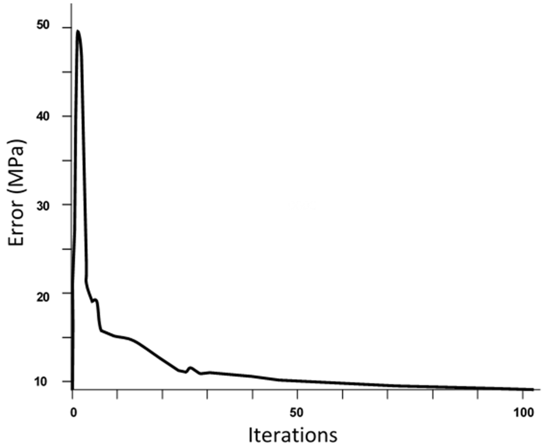
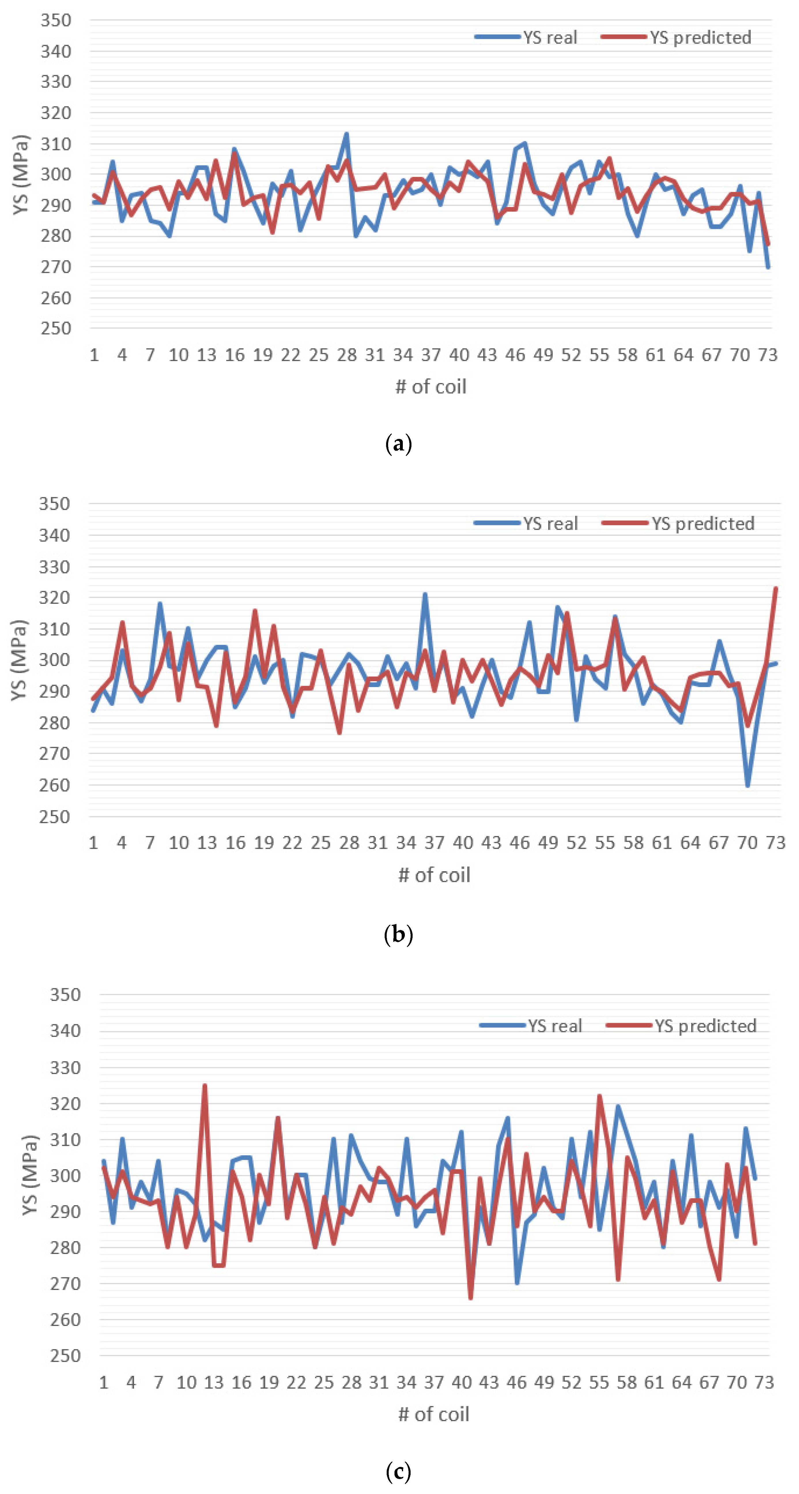
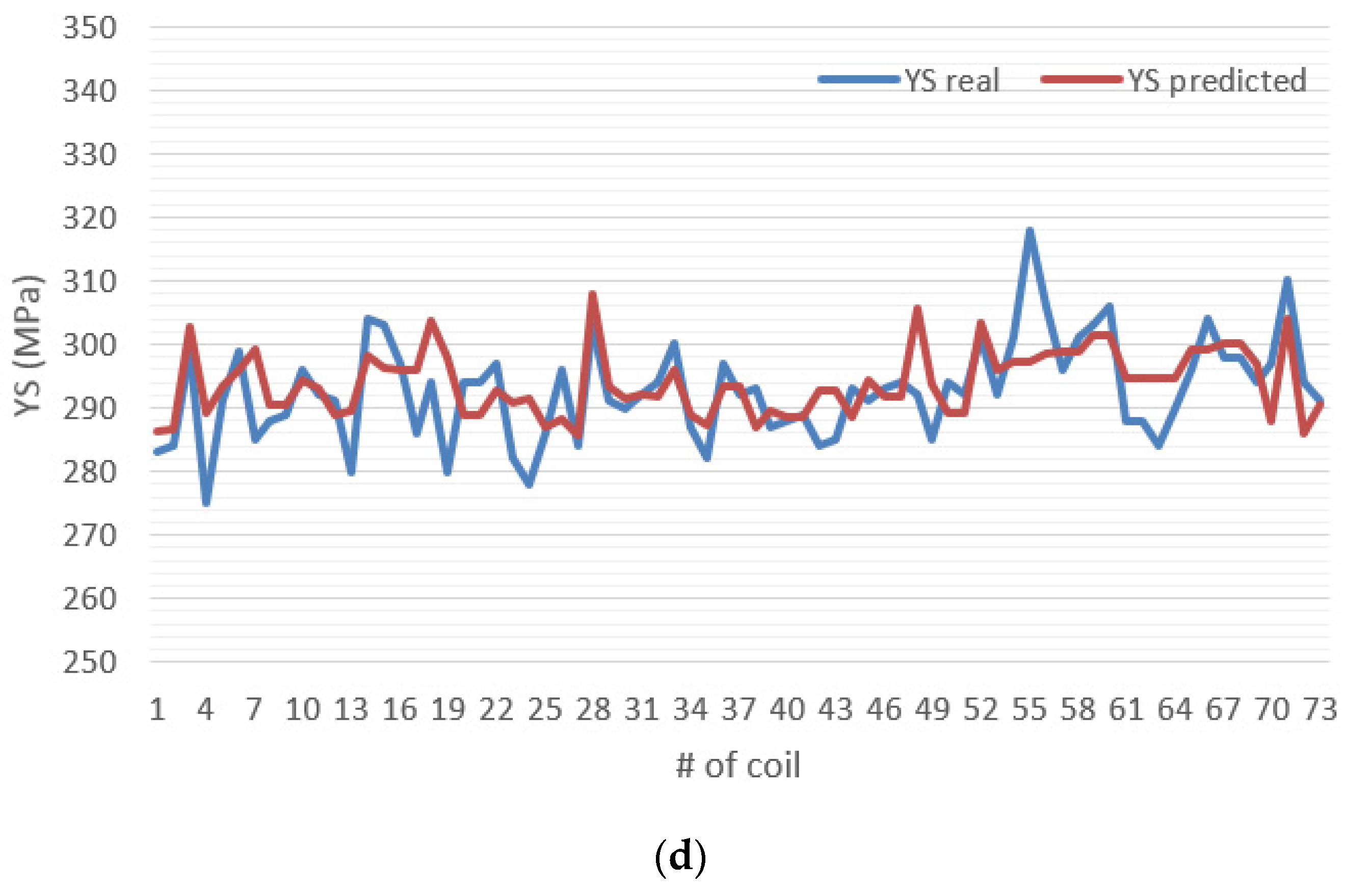
The results of the tested models are satisfactory since the errors are below 11 MPa, which is aligned with the obtained in other studies [29]. It can also be observed that the MAE is quite similar using the four different models; the reduced number of samples could be a drawback for improving the accuracy of some of these models. It is also observed that the trend of obtaining errors in the prediction of the UTS in the case of HSLA260 is lower than in case of HSL300. It seems that the difference is more related to the stability of this property in this grade than to the number of samples, because the errors in the prediction of the YS are similar for both steel grades.

The linear regression shows a significant improvement with the addition of the time–temperature parameter of up to 20%. By definition, it assumes a linear relationship between the predictors and the target variable, but the addition of the time–temperature parameter, which is an interaction parameter between speed and temperature, helps to improve the accuracy by reducing the error up to 18% in one of the datasets. The polynomial regression shows a similar performance than the linear, with an error reduction of 23% in one of the datasets with the use of the time–temperature parameter.

A better performance of the neural network and MARS models could be expected because they should model with better accuracy the complex relations between chemistry and the effect of the process parameters, but the lack of a dataset large enough could be the reason for the similarity of their results with those obtained with regressions. The use of the time–temperature parameter achieves a reduction of up to 16% in the case of the neural networks; meanwhile, the maximum improvement is only 3% in the case of the MARS.

Therefore, in an industrial environment where the size of the dataset could be limited, it makes more sense to focus the efforts in defining parameters that can provide additional information in order to improve the results of the predictions. It has also been proven that the accuracy slightly increases by using the process data in the sampling area, so that could be interesting to improve the traceability of the samples in the upstream processes to get better results.

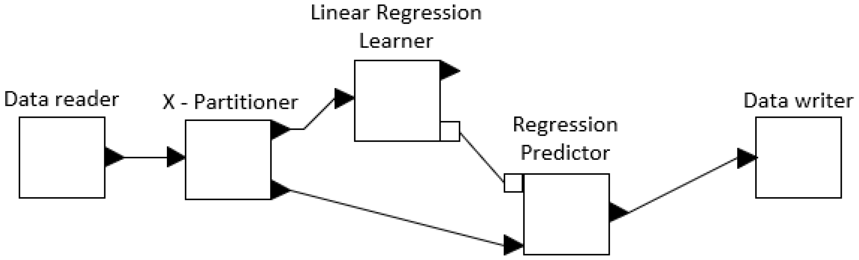
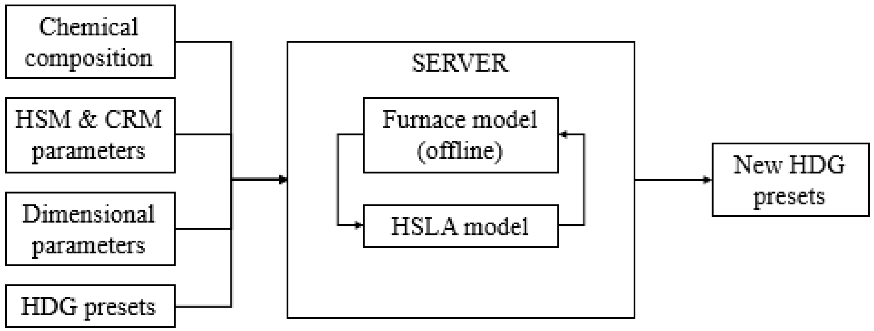
The integration of these prediction models in the production requires the architecture shown in Figure 8—the input parameters related to the upstream installations (chemical composition, hot and cold-rolling parameters, dimensional parameters) are fixed, but the parameters related to the galvanizing process are preset. As the developed models estimate the values of YS and UTS, it is possible to assess if the presets are optimal to reduce the scattering of the mechanical properties and consider modifying any of the process values (like speed, temperature, skin-pass parameters) if a quality risk is detected.

Since not all of these parameters are completely independent in the sense that the own limitations of the furnace (heating capacity and the maximum speed of the line for example) or the interrelation between them (changes in the temperature or speed will modify the value of the time–temperature parameter), it is necessary to include in the architecture an element which provides the required consistency. In this case, the HSLA models are coupled with a furnace model developed in-house [30]. The aim is to avoid inconsistencies in the results, and in case of modifying any parameter of the furnace, the rest of them are also recalculated and used in the calculations of the HSLA model.

As both, the upstream process values and the presets foreseen for the HDG line, are known in advance, it is possible to make an evaluation of the full program of coils in advance in a server and, in the case that it is needed, modify the presets to be sent to the control of the line. As the calculation time is reduced, if some of the proposed changes create abrupt transitions between coils, the line staff can decide to either reorganize the program or remove a coil from it.

5. Conclusions

The values of YS and UTS for HSLA coils produced without the soaking phase in the HDG line have been modeled using the chemical composition of the steel and the main process parameters from hot rolling to downstream. The results of four types of data-driven models have been compared for two different steel grades. The improvement of the results was evaluated using the average process values versus values in the sampling area and the effect of the addition of a new control parameter defined for the HDG line.

The overall conclusion is that for both grades, the simpler solution as a linear or polynomial regression can be used with good results. It was also confirmed that adding the time–temperature parameter helps to reduce the error in all cases, being obtained improvements over 10% in most of the cases. These models can be used to calculate, in advance, the values of the YS and UTS for each coil, and if coupled with a furnace model, it is possible to modify the presets in the HDG line and reduce the number of rejected coils.

References

1. Garcia-Martino, A.; Fernández, S.; Santiago, J.; Prieto, M.M. The consequences of eliminating the soaking section of a commercial hot-dip galvanising line for HSLA production and a control strategy for improving product consistency. Ironmak. Steelmak. 2019, 1–7. [Google Scholar] [CrossRef]
2. Hodgson, P.D.; Gibbs, R.K. A Mathematical model to predict the mechanical properties of hot rolled C-Mn and microalloyed steels. ISIJ Int. 1992, 32, 1329–1338. [Google Scholar] [CrossRef] [Green Version]
3. Orta, A.H.; Kayabasi, I.; Senol, M. Prediction of mechanical properties of cold rolled and continuous annealed steel grades via analytical model integrated neural networks. Ironmak. Steelmak. 2019, 1–10. [Google Scholar] [CrossRef]
4. Bahrami, A.; Anijdan, S.H.M.; Ekrami, A. Prediction of mechanical properties of DP steels using neural network model. J. Alloys Compd. 2005, 392, 177–182. [Google Scholar] [CrossRef]
5. Datta, S.; Banerjee, M.K. Certainty Factor Estimation Using Petri Neural Net for HSLA Steel. ISIJ Int. 2005, 45, 121–126. [Google Scholar] [CrossRef] [Green Version]
6. Datta, S.; Banerjee, M.K. Mapping the input–output relationship in HSLA steels through expert neural network. Mater. Sci. Eng. A 2006, 420, 254–264. [Google Scholar] [CrossRef]
7. Mukhopadhyay, A.; Iqbal, A. Comparison of ANN and MARS in Prediction of Property of Steel Strips. In Applied Soft Computing Technologies: The Challenge of Complexity; Springer Science & Business Media: Berlin/Heidelberg, Germany, 2006; pp. 329–341. [Google Scholar]
8. Powar, A. Modeling of microstructure and mechanical properties of heat-treated components by using Artificial Neural Network. Mat. Sci. 2015, 628, 89–97. [Google Scholar] [CrossRef]
9. Dutta, T. Designing dual-phase steels with improved performance using ANN and GA in tandem. Comput. Mater. Sci. 2019, 157, 6–16. [Google Scholar] [CrossRef]
10. Wu, S.-W.; Zhou, X.-G.; Cao, G.-M.; Liu, Z.-Y.; Wang, G.-D. The improvement on constitutive modeling of Nb-Ti micro alloyed steel by using intelligent algorithms. Mater. Des. 2017, 116, 676–685. [Google Scholar] [CrossRef]
11. Bakkaloğlu, A. Effect of processing parameters on the microstructure and properties of a Nb microalloyed steel. Mater. Lett. 2002, 56, 263–272. [Google Scholar] [CrossRef]
12. Wirth, R.; Hipp, J. CRISP-DM: Towards a Standard Process Model for Data Mining. In Proceedings of the 4th International Conference on the Practical Applications of Knowledge Discovery and Data Mining, New York, NY, USA, 27–31 August 1998; Agrawal, R., Stolorz, P., Eds.; AAAI Press: Menlo Park, CA, USA, 1998. [Google Scholar]
13. Kohonen, T.; Oja, E.; Simula, O.; Visa, A.; Kangas, J. Engineering applications of the self-organizing map. Proc. IEEE 1996, 84, 1358–1384. [Google Scholar] [CrossRef]
14. Lötsch, J.; Ultsch, A. Exploiting the Structures of the U-Matrix in Advances in Self-Organizing Maps and Learning Vector Quantization. In Proceedings of the 10th International Workshop WSOM, Mittweida, Germany, 2–4 July 2014; Villmann, T., Schleif, F.M., Kaden, M., Lange, M., Eds.; Springer: Cham, Germany, 2014. [Google Scholar] [CrossRef]
15. Sobral, M.D.C.; Mei, P.R. Effect of carbonitride particles formed in austenite on the strength of microalloyed steels. Mater. Sci. Eng. A 2004, 637, 317–321. [Google Scholar] [CrossRef]
16. Li, Y.; Crowther, D.N.; Mitchell, P.S.; Baker, T.N. The evolution of microstructure during thin slab direct rolling processing in vanadium microalloyed steels. ISIJ Int. 2002, 42, 636–644. [Google Scholar] [CrossRef]
17. Zajac, S.; Siwecki, T.; Hutchinson, W.B.; Lagneborg, R. Strengthening mechanisms in vanadium microalloyed steels intended for long products. ISIJ Int. 1998, 38, 1130–1139. [Google Scholar] [CrossRef]
18. Riva, R.; Mapelli, C.; Venturini, R. Effect of coiling temperature on formability and mechanical properties of mild low carbon and HSLA steels processed by thin slab casting and direct rolling. ISIJ Int. 2007, 47, 1204–1213. [Google Scholar] [CrossRef] [Green Version]
19. Patel, J.K.; Wilshire, B. The challenge to produce consistent mechanical properties in Nb-HSLA strip steels. J. Mater. Process. Technol. 2002, 120, 316–321. [Google Scholar] [CrossRef]
20. Janošec, M.; Schindler, I.; Vodárek, V.; Palát, J.; Rusz, S.; Suchánek, P.; Rüžička, M.; Místecký, E. Microstructure and mechanical properties of cold rolled, annealed HSLA strip steels. Arch. Civ. Mech. Eng. 2007, 7, 29–38. [Google Scholar] [CrossRef]
21. Grassino, J.; Vedani, M.; Vimercati, G.; Zanella, G. Effects of skin pass rolling parameters on mechanical properties of steels. Int. J. Precis. Eng. Manuf. 2012, 13, 2017–2026. [Google Scholar] [CrossRef]
22. Chen, J.; Shen, X.; Jin, F.; Tang, S.; Liu, Z.; Wang, G. Effect of annealing time on microstructure and mechanical properties of cold-rolled niobium and titanium bearing micro-alloyed steel strips. J. Iron Steel Res. Int. 2013, 20, 86–92. [Google Scholar] [CrossRef]
23. Raji, N.A.; Oluwole, O.O. Effect of Soaking Time on the Mechanical Properties of Annealed Cold-Drawn Low Carbon Steel. Mater. Sci. Appl. 2012, 3, 513–518. [Google Scholar] [CrossRef] [Green Version]
24. Huo, X.; Mao, X.; Lü, S. Effect of annealing temperature on recrystallization behaviour of cold rolled Ti-microalloyed steel. J. Iron Steel Res. Int. 2013, 20, 105–110. [Google Scholar] [CrossRef]
25. Specht, D.F. Probabilistic neural networks. Neural Netw. 1990, 3, 109–118. [Google Scholar] [CrossRef]
26. Lewis, P.A.W.; Stevens, J.G. Nonlinear Modeling of Time Series Using Multivariate Adaptive Regression Splines (MARS). J. Am. Stat. Assoc. 1991, 86, 864–877. [Google Scholar] [CrossRef]
27. Knime Analytics Platform. Available online: https://www.knime.com/knime-analytics-platform (accessed on 25 April 2020).
28. MARS®—Multivariate Adaptive Regression Splines. Available online: https://www.salford-systems.com/products/mars (accessed on 25 April 2020).
29. Hodgson, P.D. Microstructure modelling for property prediction and control. J. Mater. Process. Technol. 1996, 60, 27–33. [Google Scholar] [CrossRef]
30. Garcia-Martino, A.; Prieto, M.M. Practical Thermal Model for a Radiant Tubes Annealing Furnace. Metall. Res. Technol. 2020, 117, 119. [Google Scholar] [CrossRef] [Green Version]
Figure 1. Layout of the annealing furnace, and thermal profiles of the strip with soaking (a) and without soaking (b). The value of the temperature-time T-t parameter is the area indicated by the shaded area (T-t).
Metals 10 00561 g001
Figure 2. Stages of the process.
Metals 10 00561 g002
Figure 3. Output of the Self-Organized Maps (SOM) analysis for the initial set of parameters.
Metals 10 00561 g003
Figure 4. Diagram block of the linear predictor.
Metals 10 00561 g004
Figure 5. Diagram of the MultiLayer Perceptron (MLP).
Metals 10 00561 g005
Figure 6. Evolution of the error with the number of iterations.
Metals 10 00561 g006
Figure 7. Plots of the real yield strength YS and the predicted YS calculated with the test dataset 2B for: (a) linear learner, (b) polynomial learner, (c) Neural Network learner, and (d) Multivariate Adaptive Regression Splines MARS learner.
Metals 10 00561 g007aMetals 10 00561 g007b
Figure 8. Integration for the HSLA model in the process workflow.
Metals 10 00561 g008