Variation Rate to Maintain Diversity in Decision Space within Multi-Objective Evolutionary Algorithms †


1
Computer Science Department, Cinvestav-IPN, Mexico City 07360, Mexico
2
Dr. Rodolfo Quintero Ramirez Chair, UAM Cuajimalpa, Mexico City 05370, Mexico
*
Authors to whom correspondence should be addressed.
†
This paper is an extended version of our paper published in the 10th International Conference on Evolutionary Multi-Criterion Optimization (EMO 2019), East Lansing, MI, USA, in 10–13 March 2019.
Math. Comput. Appl. 2019, 24(3), 82; https://doi.org/10.3390/mca24030082
Submission received: 30 July 2019
/
Revised: 10 September 2019
/
Accepted: 11 September 2019
/
Published: 13 September 2019
(This article belongs to the Special Issue Numerical and Evolutionary Optimization)
Abstract
:The performance of a multi-objective evolutionary algorithm (MOEA) is in most cases measured in terms of the populations’ approximation quality in objective space. As a consequence, most MOEAs focus on such approximations while neglecting the distribution of the individuals of their populations in decision space. This, however, represents a potential shortcoming in certain applications as in many cases one can obtain the same or very similar qualities (measured in objective space) in several ways (measured in decision space). Hence, a high diversity in decision space may represent valuable information for the decision maker for the realization of a given project. In this paper, we propose the Variation Rate, a heuristic selection strategy that aims to maintain diversity both in decision and objective space. The core of this strategy is the proper combination of the averaged distance applied in variable space together with the diversity mechanism in objective space that is used within a chosen MOEA. To show the applicability of the method, we propose the resulting selection strategies for some of the most representative state-of-the-art MOEAs and show numerical results on several benchmark problems. The results demonstrate that the consideration of the Variation Rate can greatly enhance the diversity in decision space for all considered algorithms and problems without a significant loss in the approximation qualities in objective space.
1. Introduction
In many areas such as Economy, Finance, or Industry, the problem arises naturally that several conflicting objectives have to be optimized concurrently [1,2]. Such problems are called multi-objective optimization problems (MOPs) in literature [3,4,5]. The solution set of an MOP (in decision space) is called the Pareto set and its image (defined in objective space) the Pareto front. One important characteristic of continuous MOPs is that their Pareto sets and fronts typically form ()-dimensional objects, where k is the number of objectives considered in the problem. In many applications, the Pareto front is of primary interest as it contains information about the desired qualities of each selected solution. As a consequence, almost all existing MOEAs focus on approximations in objective space while entirely neglecting the distribution of the individuals in decision space. There exist, however, also applications where the values of the solutions in decision variable space are of great importance. As an example, consider that the amount of a certain resource (i.e., the value of a variable ) used to obtain the desired quality (measured in objective space) is important. For two solutions that are equal or similar in objective space, one may prefer the one that has a lower value of . Another example is that the variable could represent the launch date of a project, as, e.g., in [6] in the context of space mission design. For such problems, different values of directly relate to different timescales in the realization of the project. In that case, the decision maker may select one “optimal” realization of the project, and keep solutions with similar objective values but later launch dates as back-up solutions. For such problems, the sole consideration of the approximation quality in objective space represents a potential shortcoming. On the one hand, it is of course possible to formulate all such problems via additional constraints and objectives. On the other hand, such re-modellations of the problem lead in general to a higher complexity compared to the original problem. For instance, by each added objective, the dimension of the Pareto set/front increases by one. Hence, in this context, there exists an additional challenge in solving a given MOP, since we have to find a suitable approximation to the optimal set both in objective and decision space, in order to provide a satisfying overview of the possible solutions to the decision maker. Another application can be found in [7], where data analysis techniques are used to discover patterns and rules. Here, authors conclude that such process of innovation by optimization (“innovization”) has an enormous potential to revolutionize the engineering of the design process in the industry.
In this paper, we propose a framework for equipping MOEAs with a mechanism that performs an exploration of both decision and objective spaces. The underlying idea of this proposal, called Variation Rate, is to measure the spread via using the averaged distance in decision space for elements for which function values are close in objective space. After discussion of the general framework, we present implementations of variants of NSGA-II [8] (elitist algorithm), SMS-EMOA [9] (indicator based algorithm), MOEA/D [10] (decomposition based algorithm), and NSGA-III [11] (designed for the treatment of MOPs with many objectives). Further on, we demonstrate the effectiveness of our approach on several benchmark problems, where we show that, compared to the base variants, we greatly improve the approximation qualities in decision space without any significant loss in the qualities in objective space. A preliminary study of this work can be found in [12], where the discussion on the proposed method is reduced, and where it has only been applied to NSGA-III.
The remainder of the paper is organized as follows: in Section 2, we briefly present the background required for the understanding of this paper and discuss the related work. In Section 3, we first present the general framework of the Variation Rate and further on provide particular implementations for four different MOEAs that are representative of the state-of-the-art. In Section 4, we present some numerical results on selected benchmark problems using both the four base MOEAs as well as their variants that use the Variation Rate. Finally, in Section 5, we discuss the advantages of the proposed approach and discuss possible paths for future research.
2. Background and Related Work
Optimization refers to finding the best possible solution to a problem given a set of constraints [4]. Multi-objective optimization refers to the simultaneous optimization of multiple and usually conflicting objectives. More precisely, a multi-objective optimization problem (MOP) with k objectives is mathematically defined as follows:
where is the domain and is called the objective function.
The optimality of an MOP is defined by the concept of strict dominance. Let , the vector v is less than w (), if for all ; the relation is defined analogously. A vector is dominated by a vector () with respect to (1) if and , else y is called non-dominated by x. A point is Pareto optimal to (1) if there is no that dominates x. The set of all the Pareto optimal points is called the Pareto set and its image is called the Pareto front. Typically, i.e., under certain mild smoothness assumption on the model, both Pareto set and front form at least locally ()-dimensional objects.
Unlike evolutionary algorithms for single objective optimization problems (SOPs), maintaining diversity in decision space is not a priority for most MOEAs; most of the performance indicators are developed in order to measure the accuracy based only on the objective function (e.g., the hypervolume [13] and the Degree of Approximation [14]). As exceptions, we have some of the measures used for multimodal optimization (see [15]) and two particular examples. The first one is the indicator [16,17], which can be viewed as an averaged Hausdorff distance and which actually measures the distance between two general sets and we can use it as an indicator both in objective space as well as in decision space. The other work that can deal with this aspect is the diversity integrating multiobjective optimizer (DIOP) [18], which is user-defined and concurrently optimizes two set-based diversity measures, one in decision space and the other in objective space. In this work, the relationship between the two set-based diversity measures is conceived as a bi-objective optimization problem and it is solved via a weighted sum of the two diversity indicators. In particular, the authors consider the Solow–Polasky measure as it satisfies three requirements: monotonicity in varieties, twinning, and monotonicity in the distance.
Although works that explicitly consider at the same time variables and objectives are scarce, one can find some related work on this topic in [19] and some specific algorithms. For instance, the NSGA [20] (the algorithm that precedes the well-known NSGA-II) uses fitness sharing in decision space. In [21], some possible techniques are proposed to spread out solutions both in objective and decision decision space: pointwise expansion, threshold sharing, sequential sharing, simultaneous sharing multiplicative, and simultaneous sharing additive. It is important to point out that the above approaches are only part of the discussion of the paper and they were not implemented; the implemented algorithm was the Niched Pareto GA, a method with phenotypic sharing. In addition, all of the described techniques depend on the normal fitness sharing method, that is, two additional parameters must be provided or approximated (the niche radius in both decision and objective spaces).
The omni-optimizer algorithm [22] is proposed as a procedure that aims at solving a wide variety of optimization problems (single or multi-objective and uni- or multi-modal problems). The authors argue that, to solve different kinds of problems, it is necessary to know different specialized algorithms. Thus, it is desirable to have an algorithm that adapts itself for handling any number of conflicting objectives, constraints, and variables. The omni-optimizer is important in the context of this work as it uses a two-tier fitness assignment scheme based on the crowding distance of the NSGA-II. The primary fitness is computed using the phenotypes (objectives and constraint values) and the secondary fitness is computed using both phenotypes and genotypes (decision variables). The modified crowding distance computes the average crowding distance of the population in objective and decision spaces. If the crowding value for some individual is above average (at any space), it is assigned the larger of the two distances; otherwise, the smaller of the two distances is assigned. However, we must not lose sight of the fact that omni-optimizer was developed not only to maintain diversity in decision space but with a more general purpose (it adapts itself to solve different kinds of problems).
An algorithm that explicitly promotes the diversity of the decision space is the MOEA/D with Enhanced Variable-Space Diversity (MOEA/D-EVSD), proposed in [23]. This method is an extension of the MOEA/D [10] but with an enhanced variable-space diversity control. In the first generations, the MOEA/D-EVSD tries to induce a larger diversity via promoting the mating of dissimilar individuals. Similarly to MOEA/D, a new individual is created for each subproblem. Then, instead of randomly selecting two individuals of the neighborhood, a pool of candidate parents is randomly filled from the neighborhood with probability , and with probability from the whole population. The two selected parents are the ones in the pool that have the largest distance among them. As the parameter is dynamically set, a gradual change between exploration and exploitation can be induced. Additionally, a final phase to further promote intensification is included, which is essentially a traditional MOEA/D coupled with Differential Evolution (DE) operators. For the last generations of MOEA/D-EVSD, the traditional mating selection of MOEA/D is conserved together with the Rand/1/bin scheme for the DE operators. The authors of this paper show that, by inducing a gradual loss of diversity in the decision space, the state-of-the-art of MOEAs can be improved.
Finally, in [24], the diversity integrating hypervolume-based search algorithm (DIVA) is proposed. Here, the authors proposed a modified hypervolume indicator, which is integrated into an evolutionary algorithm. They employ a so-called diversity function, which fulfills certain requirements such that the modified hypervolume indicator remains compliant with the underlying preference relation.
3. Proposed Framework
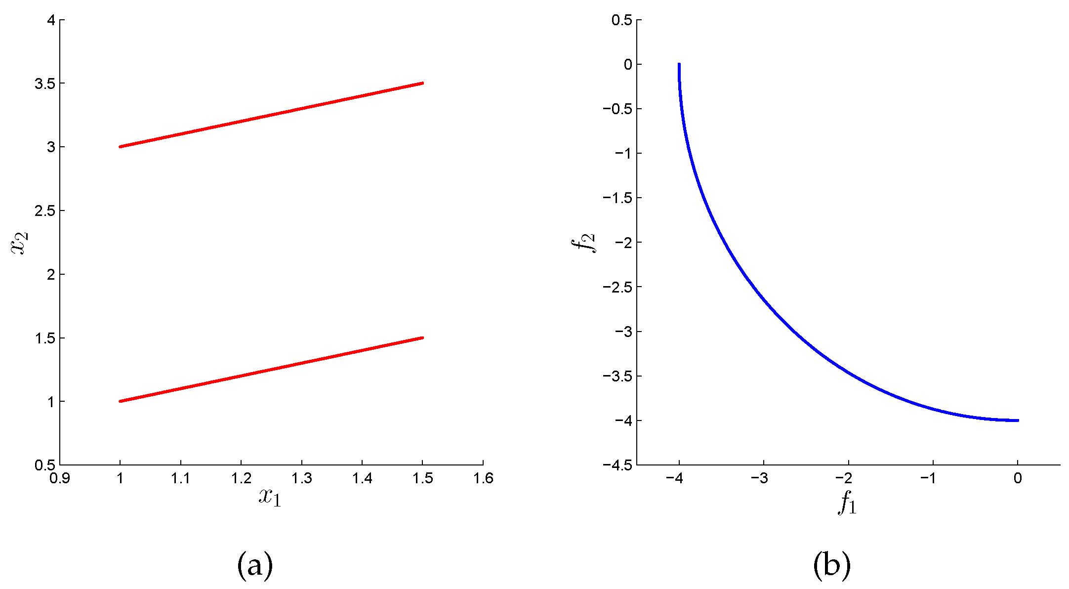
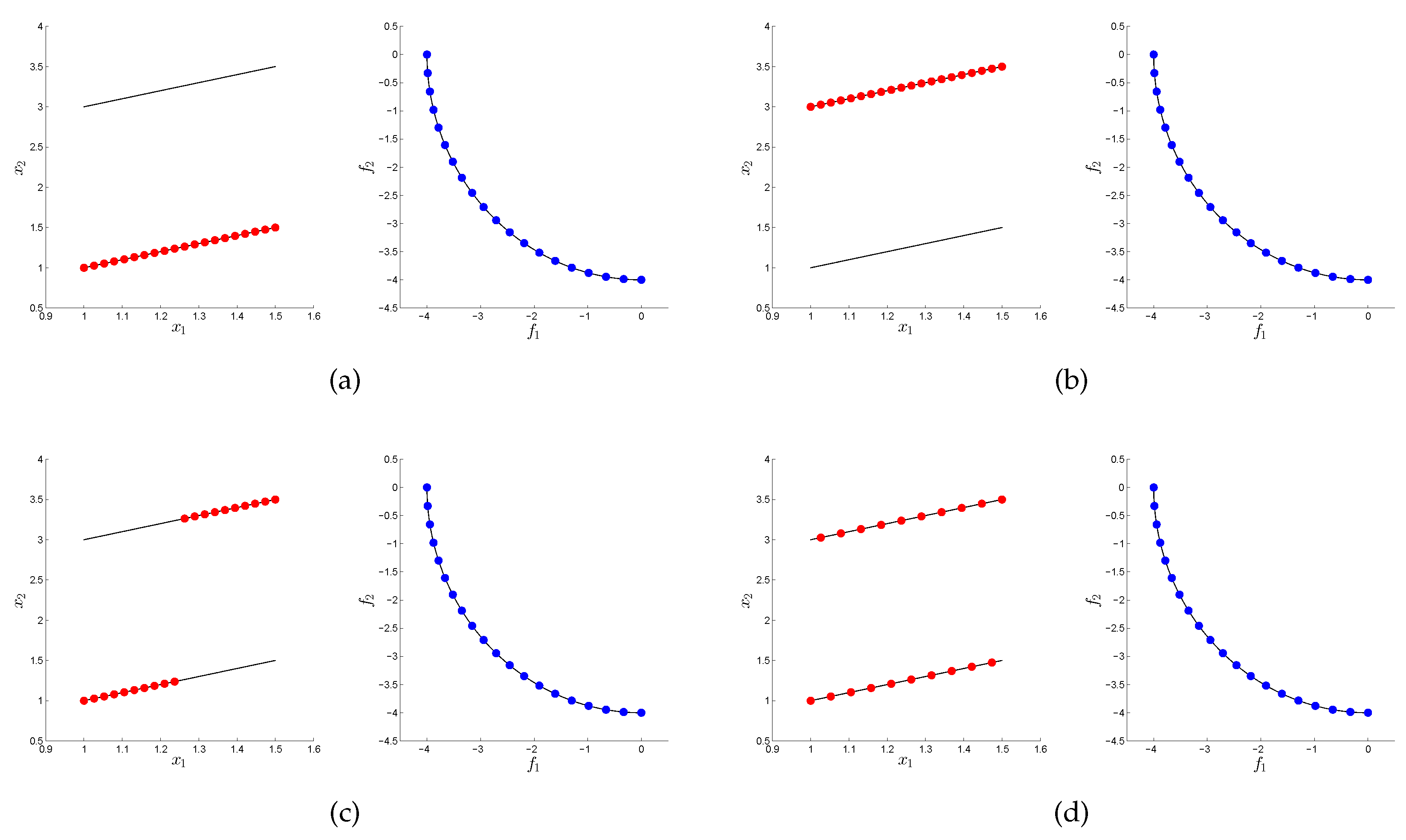
State-of-the-art MOEAs that measure the approximation quality of their outcome entirely in objective space work typically well if there is a 1:1 relationship between Pareto set and Pareto front (that is, if, for every , there exists exactly one such that ). That is, if a good finite size approximation of the Pareto front is found by the MOEA (the goodness can be measured, e.g., by any existing performance indicator), the respective finite size approximation of the Pareto set is in many cases also satisfying. This, however, does not hold any more if there is an relationship between Pareto set and front (i.e., if there are multiple such that for a ). If, for instance, there are several connected components of the Pareto set that map to the same part of the Pareto front, a good Pareto front approximation does not imply a good (or at least satisfying) approximation of the Pareto set. To see this, consider the hypothetical bi-objective problem that is shown in Figure 1. The Pareto set of this problem consists of two disjunct connected components that map both to the same Pareto front (that is, every has exactly two pre-images). Figure 2 shows four possible approximations in decision and objective space. As it can be seen, the approximation quality is very high for all sets in objective space, while this is not the case for the Pareto set approximations. Out of them, only the last one is “complete” according to the given discretization. MOEAs that merely measure their outcomes in objective space cannot distinguish between those solutions, and, consequently, the Pareto set approximation is left to chance. MOPs of this kind are termed Type III problems in [25].
To overcome this problem, we propose to perform a density estimator that aims to obtain a good distribution both in objective and decision space. Usually, a classical density estimator groups the population considering only the objective values. Such classification is commonly used to define selection criteria for its elements, giving them certain reference value based on its distribution in objective space. According to the design of each algorithm, the individual with either lower or higher reference value is chosen. The idea is to define a relationship between this reference value in objective space and a certain measurement in decision space. In this way, the first grouping phase identifies promising solutions in objective space; meanwhile, the second phase favors solutions with the most different values in the decision space. Our goal is to properly represent the trade-off between these two aspects.
3.1. Using the Averaged Distance in Variable Space
In the following, we discuss why we think that the usage of the averaged distance is an adequate measure in decision space that serves our purpose.
Let be a finite set, then the averaged distance between each element and the rest of the elements in I is given by
where is the desired metric for the distance between the two elements and in the decision space that can vary according to the codification or the used norm. In this work, we consider the Euclidean distance, i.e., .
Though the averaged distance is defined for every finite set , we will apply it on sets where the values of their images, , are close to each other.
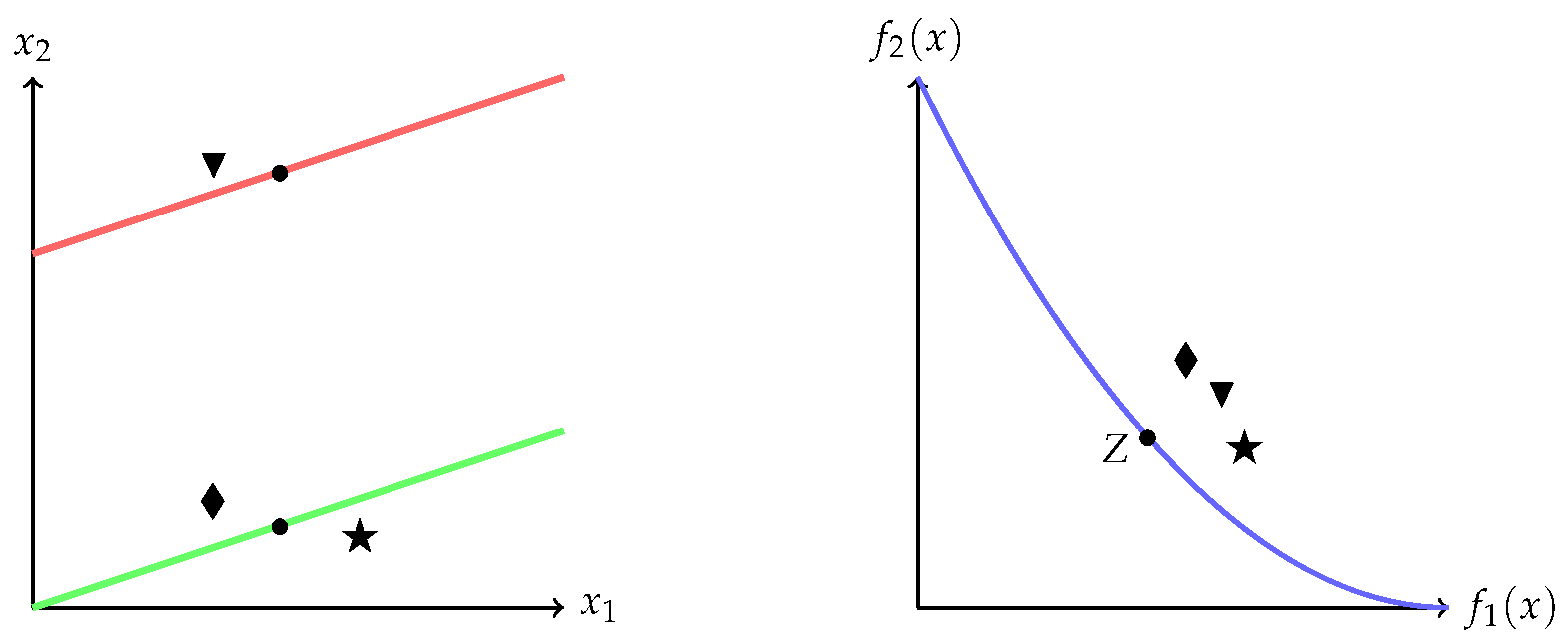
As an illustrative example, consider again the Type III bi-objective problem whose Pareto set and front are shown in Figure 3. The set I is given by the three points ▾, ⧫, and ★. All three images are relatively close to the given reference point Z point Z in objective space; assume, for simplicity, that the distances of all three images to Z are given by one (i.e., = = = 1). Furthermore, we assume that, for the distances in variable space, we have , , and . Then, we obtain
Notice that the point with the biggest average distance in variable space is also the most different individual in this space. In other words, elements with the maximum average distance in decision space have the desired behavior for Type III problems.
However, it is not sufficient to only take into account the average distance of the variables as a selection criterion. Our problem now is how to select an individual that has both a good quality in objective space as well as a good distribution in variable space. We discuss this issue in the following.
3.2. Variation Rate
As explained before, the generic selection criterion of most MOEAs prefers individuals with “the best” reference value in objective space, and this could be a maximum or a minimum value according to the selection procedure. For instance, the selection criterion of the NSGA-II prefers individuals with the biggest crowding distance, while the niching procedure of the NSGA-III favors individuals with the least distance to an induced line. On our part, we have to consider both the reference value provided by the classical selection criterion, as well as the average distance in variables to solve Type III problems.
We first consider selection mechanisms that prefer small reference values. For this, let I be a set of points in decision space whose images are close to each other, let be the reference value in objective space for each and let as defined as in (2) (in decision space). Then, the variation rate for each element is stated as follows:
This makes sense because for Type III problems the elements of the neighborhood I will have a similar reference value in objectives while the average distances will be larger for the most different solutions in decision space. Hence, its quotient (the variation rate) will tend to be smaller than for the rest of the quotients. Thus, through the variation rate, we have a way to relate the objective and the decision spaces in order to choose the best individual in each group.
Next, we address selection mechanisms that prefer large reference values. For this, we have two options. The first one is to edit the selection criterion to prefer small values in order to use the variation rate. The second alternative is to use a product instead of a quotient. We decide to conserve the essence of each MOEA; for this reason, we implement the second option in this work, which we call the inverse variation rate. More precisely, for a set I as above with reference values for each and as defined in (2), the inverse variation rate is defined as follows:
Using this definition, elements with the largest values are hence preferred.
In order to illustrate these two approaches, we go back to the example shown in Figure 3 where we already have the values of and for all the three elements of the set I. Suppose that we have to select two out of the three individuals ★, ▾, and ⧫.
If we work with an MOEA that has a selection criterion that prefers individuals with the least distance to Z in objective space, then the only option we have is randomly choosing them (since , , and ). However, if we use the variation rate, then the values change to:
In this way, we select ▾ as the preferred solution and the second one is ★, which preserves individuals in both of the disconnected regions in decision space.
The desired two-element population is hence given by
Otherwise, if we work with an MOEA that has a selection criterion that prefers individuals with the largest distance to Z in objective space (maybe in order to preserve diversity), then the option we have again is randomly choosing two of them. However, if we use the inverse variation rate, that is:
then it also leads ▾ and ★ as the selected individuals.
The desired two-element population is again given by
Observe that, in both cases, we conserve one individual in each disconnected component of the Pareto set. This is something that we can not guarantee with the use of a standard approach.
Notice that, for all MOPs with a 1:1 relationship of the Pareto set and the Pareto front, it is expected that solutions in the same neighborhood have similar reference values in objective space and also a similar average distance in decision space. Thus, it is also likely that making the quotient or the product of these values does not significantly affect the original selection criterion. This will be shown in Section 4 on several classical benchmark problems.
We can now state a general framework. A pseudocode of the Variation Rate is shown in Algorithm 1.
| Algorithm 1 Framework to include the Average Distance in Variables within any MOEA |
| Require: Parameters of the selected MOEA Ensure: Final population
|
In Algorithm 1, the procedure SelectByVariationRate takes the reference values in objective space provided by SelectProcedure (we assume it is based on a classical selection criterion), and then it updates such values according to the variation rate or the inverse variation rate in order to improve the selection mechanism to deal with Type III problems.
As we can see, this framework can be used in principle within any MOEA; however, the particular use of the variation rate or the inverse variation rate will depend on the given MOEA. In the following, we explain how to adapt the Variation Rate for four of the most representative MOEAs. The reader can find the pseudocode of these four variants in Appendix A.
3.3. Integration into NSGA-II
The first algorithm that we consider is the classical NSGA-II, which has been used successfully for the treatment of a large number of applications. This is a domination-based multi-objective evolutionary algorithm; that is, this method directly applies the Pareto dominance relation and an elitism strategy to preserve the best individuals along the optimization process. The elitism operator is incorporated via a special parent selection based on two mechanisms: fast-non-dominated-sorting and crowding distance. The former conserves best individuals based on the Pareto dominance relation, whereas the latter is used to promote the preservation of the diversity.
We consider the classification in fronts performed by the fast-non-dominated-sorting as our neighborhood structure because the crowding distance is applied only in the last front that can contribute elements to the next population. This means that we have to integrate the diversity into decision space into the crowding distance. The crowding distance procedure sorts the elements in the last front according to the values of objectives; then, the crowding distance of an individual is the average distance in objective space from the previous and the next individuals (according to the induced order), that is, the individuals and the . In order to preserve the extreme individuals, the crowding distance of the first and the last element is set as a big value. This means that the crowding distance prefers elements with big values, and, hence, we use the inverse variation rate.
The pseudocode of the modification of the NSGA-II with the variation rate (VR-NSGA-II) is shown in Algorithm A1 of Appendix A.1.
3.4. Integration into NSGA-III
We consider this algorithm here because it is able to properly deal with MOPs with many objectives. This algorithm is similar to its predecessor, the NSGA-II in the variation operators and in the classification of the fronts via the fast-non-dominated-sorting; however, the crowding distance is replaced by a more sophisticated procedure.
Here, the idea is to take advantage of the association method of the NSGA-III, which defines a “neighborhood” structure in a very convenient way for our purpose. The association method assigns each element of (the last front classified after the fast-non-dominated-sorting) to the nearest induced line by some weight , where Z is a set of reference points. Each weight can have more than one associated element, forming a neighborhood.
In the original NSGA-III, the niching is realized by sorting the obtained groups in the association stage according to its cardinality in ascending order. The element with the least distance to the induced line in each group is selected, and the algorithm continues with the next group until the population is filled. Thus, we modify the niching method. To include the diversity in decision space, our new niching procedure does not prefer the element with the least distance value. Instead, it prefers the one with the smallest variation rate.
The pseudocode of an iteration of the VR-NSGA-III algorithm with variation rate is shown in Algorithm A2 of Appendix A.2.
3.5. Integration into MOEA/D
MOEA/D is part of the Decomposition-Based Evolutionary Algorithms, which transform the original multi-objective optimization problem into a set of single-objective optimization problems that are simultaneously solved. In particular, this method takes a set of weights to define neighborhoods. The set of nearest weights defines one neighborhood and the best individuals are selected based on the value of a certain aggregative function. MOEA/D considers the weighted aggregation of objectives as an elitism mechanism. Furthermore, the neighborhood structure promotes the mating of close solutions. Different aggregative functions can be used in the MOEA/D framework, However, individuals with the least values are selected. In this work, we employ the Tchebycheff function, which is the most popular approach.
In order to include variation rate to the MOEA/D, we modify the selection criterion. Instead of preferring individuals with the least aggregative function value, we use the least value of the variation rate. For this, we employ the neighborhood structure of the original MOEA/D.
The pseudocode of VR-MOEA/D is shown in Algorithm A3 of Appendix A.3.
3.6. Integration into SMS-EMOA
SMS-EMOA is an indicator based algorithm; this means that it uses as a selection criterion the value of a certain performance indicator. In the case of SMS-EMOA, it is the hypervolume indicator.
This algorithm is similar to the NSGA-II, but it replaces the crowding distance by the contribution to the hypervolume of each individual in the last front. That is, the individuals of the last front with the biggest contribution to the hypervolume are preferred.
In this case, to adapt the SMS-EMOA, we consider the inverse variation rate, as the original mechanism criterion of this algorithm prefers high values. Again, we use the last front as our neighborhood structure.
The pseudocode of this method is shown in Algorithm A4 of Appendix A.4.
4. Numerical Results
In this section, we show some numerical results and comparisons to the state-of-the-art to demonstrate the benefit and strength of the variation rate. To this end, we first compare the original version of each algorithm against its corresponding version that uses the variation rate (respectively, the inverse variation rate) on some widely used (non-Type III) benchmark problems. This is done in order to show that the performance of each algorithm is not significantly affected for standard problems. In the next step, we test again the original and variation rate versions of the selected MOEAs on some Type III problems, where the advantage of the variation rate becomes apparent.
The benchmark problems that we use for the first part of these experiments are the well known test problems DTLZ 1-4 [26], IDTLZ 1 and IDTLZ2 [27], as well as the test problems WFG 1-5 [28]. For the second part, we use following six Type III problems.
The first Type III problem is taken from [22], which is defined as follows:
where . This problem, denoted as OMNI1 in this work, has a total of 243 different disconnected components that form the Pareto set, and all of these components map to the same Pareto front.
The second problem, also taken from [22], is defined as follows:
where , and . This problem is denoted as OMNI2 in this work. Let be the sum of the variables, then the Pareto set consists of the points x where or . In addition, here, both connected components map to the same Pareto front. That is, every point on the Pareto front can be obtained in different infinite ways via the combinations of the variables mentioned.
The third Type III problem is the application stated in [29,30], where subdivision techniques have been used to tackle the problem. It is stated as follows: for , it is:
where
Finally, we consider the methodology from [25] to construct three more problems, denoted in this paper as RPH1, RPH2, and RPH3. These are bi-objective problems with two variables. In order to properly define them, we use the following functions.
First, we define the objective functions for the RPH1-3 problems
where and . The variants of the RPH problems are obtained with the following functions.
Let and , with , be the tile identifiers that are determined via:
which restrict the problem to nine tiles using the relation , with .
Then, RPH1 is defined as , where is defined by the following transformation:
For the RPH1-3 problems, we fix the constant values , , and .
The RPH2 problem is defined as the RPH1, but it rotates the variables. That is, for an angle , we have
and then . In this paper, we use .
Finally, via the following transformation
for some small and where U and L denote the upper and lower bound of the search space, respectively; we can define the RPH3 as: , which is a rotated and transformed problem. In this paper, we use for the RPH3 problem, while and are the the upper and lower bounds of each variable for the RPH1-3 problems.
We use the PlatEMO platform [31] to make our test. The parameter settings of all the used algorithms are shown in Table 1. For all experiments, we have executed 30 independent runs. The numerical results with the mean and standard deviation of the hypervolume and indicators are shown in Table 2 and Table 3. In these tables, we have put in bold the best value between each pair of algorithms (the original version and the version with variation rate). We also performed the Wilcoxon test [32] as statistical significance proof to validate the results. For this, we consider the value . We put in gray the cell where such difference has statistical significance according to this test.
From the tables, we obtain that, for the classical benchmark problems, the original version of the selected MOEAs has a better value than the variation rate version in 27 out of the 44 combinations, where only 19 out of these values have statistical significance, which is an expected result. However, it is important to notice that the variation rate versions do not always lose, according to the indicator values, the variation rate versions are better in 17 out of 44 cases, but only in two with statistical significance.
For the hypervolume indicator, something similar happens. Here, the original version of the MOEAs is better than the variation rate version in 33 out of 44 runs, with statistical significance in 21 cases, while the variation rate version wins in 11 out of 44 cases for this indicator, where three of them have statistical significance.
In total, from the 88 possible combinations (algorithms, indicators and problems), we have statistical significance in 45 cases; this means that, almost 50% of the time, it is not possible to say that the original version is different than the variation rate version. Moreover, in the cases when we have statistical significance, we can see in Table 2 that the averaged values are very similar.
We observe the advantages of the variation rate versions with the Type III problems (see Table 3). For these problems, we use the both in objective and decision space (we denote this in the table as Obj. and Var. , respectively). We observe a similar behavior in objective space, here 16 out of 24 possible combinations are better for the original MOEAs (but only 6 out of these 34 have statistical significance). However, in decision space, the variation rate versions are better than the original versions; we have that 18 out of 24 combinations have better values, almost all of them with statistical significance (only, in one case, we can not reject the null hypothesis).
Graphical results are shown in Figure 4, Figure 5, Figure 6, Figure 7, Figure 8 and Figure 9; we plot the original MOEA and its corresponding variation rate version with the best value for each problem (according to the median of all runs using the Var. ).
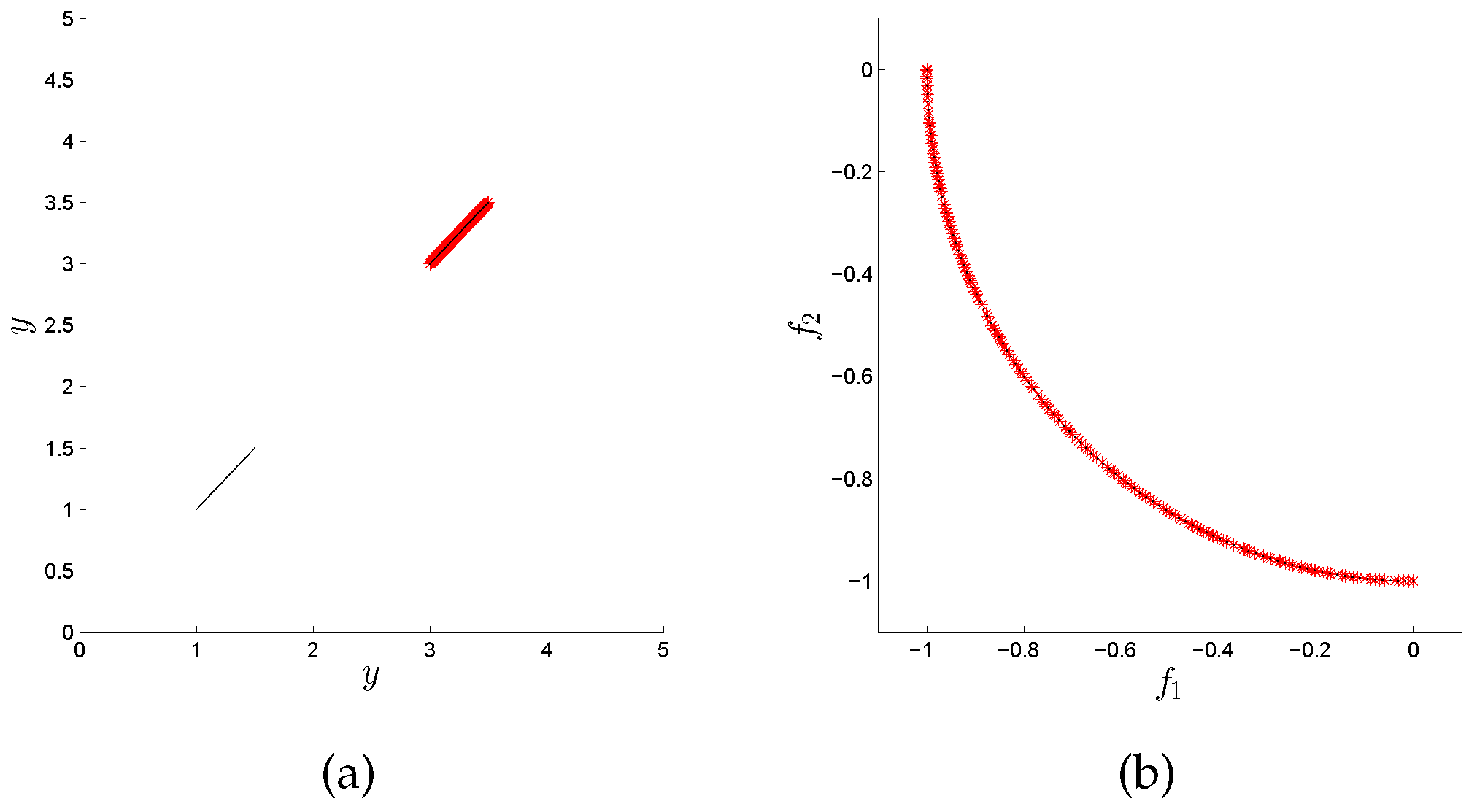
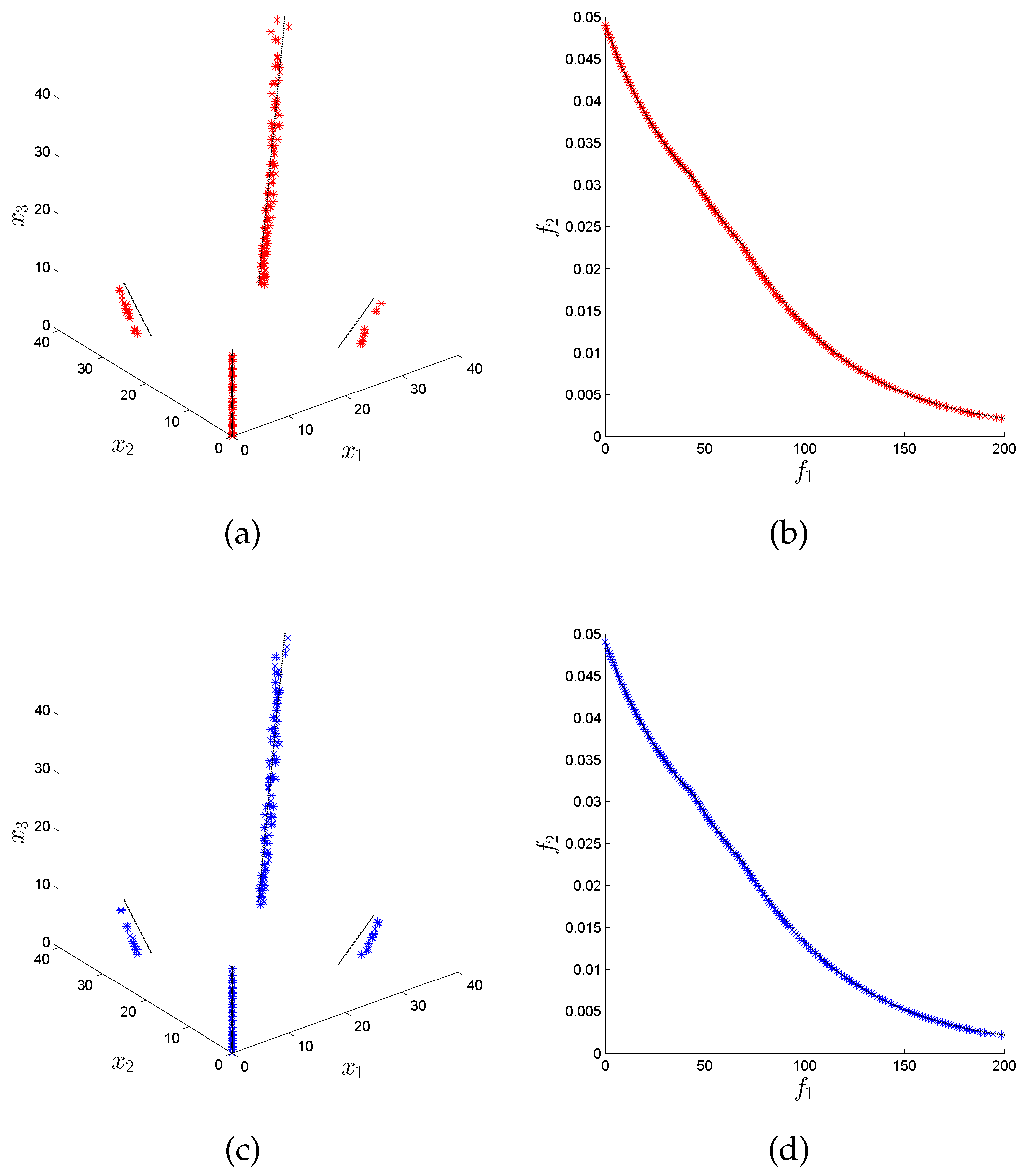
In Figure 4, we can see that the obtained distribution is better for the variation rate version; it looks similar to that obtained by the original algorithm. However, we have to recall that this problem has 243 different disconnected components in the Pareto set, and some of them are overlapping in the plot. In Figure 5, we notice that the variation rate version can obtain points at the two regions in this representation (we plot y on both axes, where ), while the original version is only able to compute points in one of them. On the other hand, in Figure 6, we can see that both the original and the variation rate versions can approximate the disconnected components of this problem well (except by the MOEA/D algorithm). However, the variation rate version is better in this problem, according to the values of Table 3.
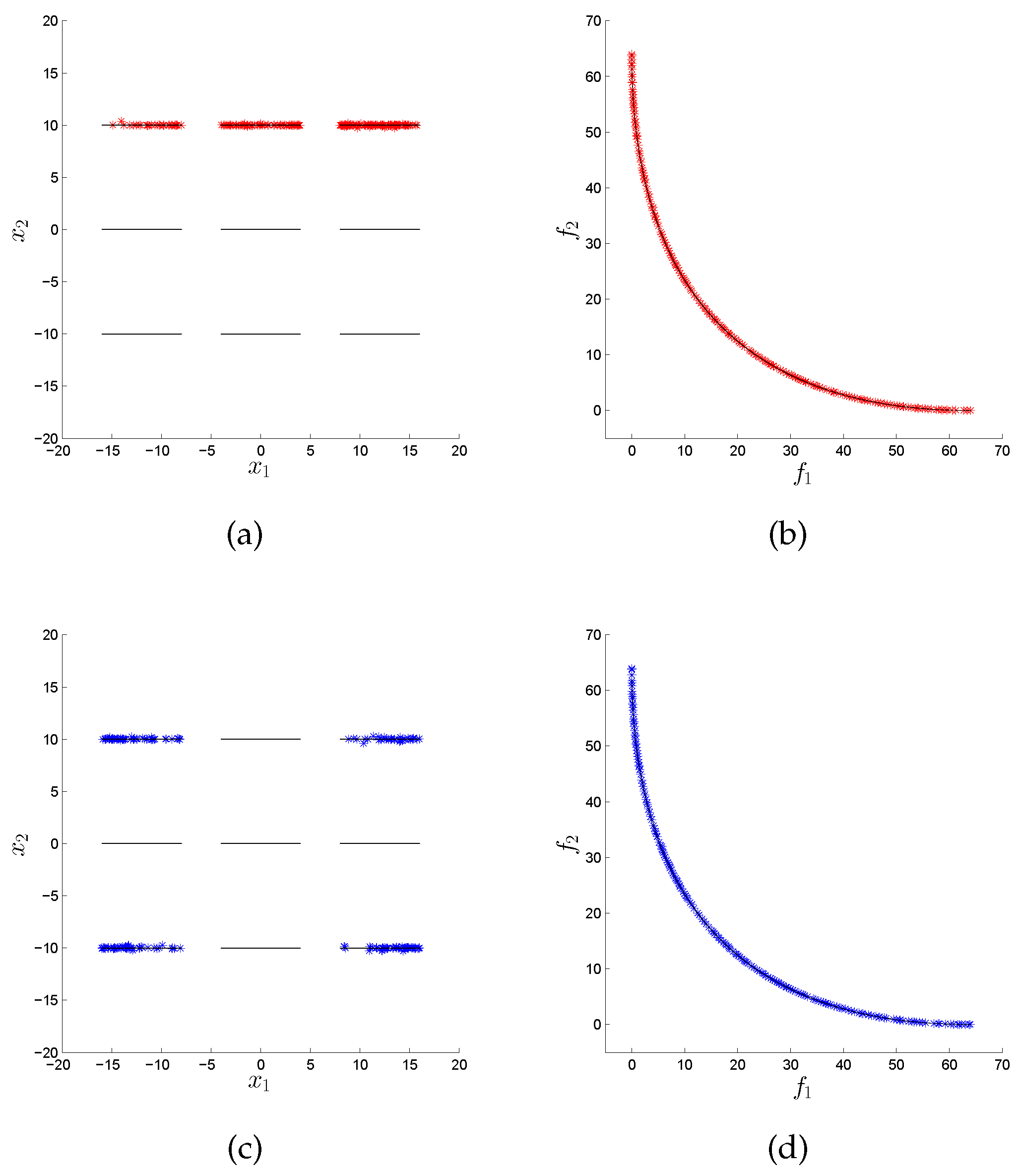
For the RPH problems, we can see in Figure 7 that the variation rate version of the NSGA-II can obtain four out of the nine disconnected components of the Pareto set, while the original version only gets three out of them; moreover, the distribution in decision space is also improved. In Figure 8, we can see again a similar behavior between the variation rate and the original version of the NSGA-III algorithm, which is also confirmed by the values of Table 3, where the variation rate version wins in three out of the four baseline algorithms for the RPH2 problem, but only in one does it have statistical significance. Finally, for the RPH3 problem, we can see in Figure 9 how the variation rate can significantly improve the performance of the MOEA/D algorithm in its distribution in decision space, as the original version only obtains points in one out of the nine disconnected components of the Pareto set, while the variation rate version obtains five out of them.
5. Conclusions and Future Work
In this work, we have addressed the problem of computing diverse solutions both in decision and objective space for a given multi-objective optimization problem via specialized evolutionary strategies. While so far quite a few good diversity mechanisms exist to obtain a spread in objective space, the consideration of the Pareto set approximations has been mainly neglected so far. This represents a possible shortcoming in particular for Type III problems where points in the Pareto front may have multiple pre-images. To achieve this goal, we have first presented the general framework of the variation rate that combines the usage of the averaged distance in variable space with the selection operator that is given by the multi-objective evolutionary algorithm (MOEAs). We have demonstrated further on possible integration of the variation rate into four MOEAs that represent the state-of-the-art.
Numerical results have shown that the use of the variation rate improves the performance of the standalone algorithms for Type III problems, while the variation rate algorithms are not significantly worse for the standard benchmark problems (i.e., problems with a 1:1 relationship between Pareto set and Pareto front), even in some cases variation rate improves the performance of the original algorithm. Of course, the behavior of variation rate by itself is not enough for the treatment of every kind of MOP as this depends on the operators of every algorithm. That is, the variation rate can enhance the overall performance of a certain algorithm, but if, for instance, such algorithm is not conceived to deal with MOPs with many objectives, the addition of the variation rate would be not enough to solve them. We can, for instance, consider some of the algorithms and test functions of [33], in order to show if the variation rate provides some advantages when dealing with MOPs with many objectives.
As future work, it will be mandatory to adapt the genetic operators of the evolutionary algorithms to exploit the diversity in decision space. As the above results have shown, the diversity in decision space has already increased significantly; however, the variation rate is only a selection mechanism. In order to obtain optimal solutions in particular in decision space, the exploration will have to be increased. Furthermore, it will be necessary to develop a particular indicator for problems of Type III. In general, performance indicators evaluate an approximation based on the value of the objectives, but, for problems such as OMNI1, this does not provide enough information. Once we have such an indicator, we can validate better performance of our methods in decision space. However, it is ad hoc not clear which property has to be satisfied with this approximation. We also need to test this approach in problems with different properties in decision space, in particular problems with disconnected Pareto sets.
Author Contributions
O.C. and O.S. conceived and designed the experiments; O.C. performed the experiments; O.C. and O.S. analyzed the data; O.C. and O.S. wrote the paper.
Funding
The authors acknowledge funding from the Conacyt Basic Science project No. 285599 and SEP Cinvestav project No. 231.
Acknowledgments
The first author acknowledges support from the Conacyt to pursue his PhD studies.
Conflicts of Interest
The authors declare no conflict of interest.
Appendix A. Pseudo-Codes
The appendix contains the pseudocode of all the variation rate algorithms that were used in this work.
Appendix A.1. VR-NSGA-II
The differences between the original NSGA-II and the VR-NSGA-II are lines 12 and 20. In line 12, we compute the inverse variation rate values of the last front, while, on line 20, we perform the selection according to these values.
| Algorithm A1 Pseudocode of VR-NSGA-II |
| Require: Population size (), crossover probability (), mutation probability ) Ensure: Final Population
|
Appendix A.2. VR-NSGA-III
We only show the iteration as the complete code is basically identical to NSGA-II with a different selection mechanism. Here, the main difference of the variation rate version, compared to the original NSGA-III, is on line 14; while the original NSGA-III uses the ninching as selection criterion, the VR-NSGA-III employs the variation rate, as it is stated on line 14.
| Algorithm A2 Iteration of the VR-NSGA-III |
| Require: Reference points Z, current population Ensure: Next, population
|
Appendix A.3. VR-MOEA/D
The change in this algorithm, concerning the original MOEAD, is very subtle. On lines 9 and 10, we compute the variation rate of the elements of the neighborhood and the offspring () instead of only computing the values of the aggregative function.
| Algorithm A3 Pseudocode of VR-MOEA/D |
| Require:N number of solutions and weight vectors; T neighborhood size. Ensure: Final Population
|
Appendix A.4. VR-MOEA/D
Again, in this case, we only show an iteration of the method as the rest of the algorithm is basically the NSGA-II. We observe that, on line 12, we substitute the values of the hypervolume contributions with the variation rate and we use them for the selection mechanism.
| Algorithm A4 Iteration of the VR-SMS-EMOA |
| Require: Current population Ensure: Next, population
|
References
- Coello, C.A.C.; Lamont, G.B. Applications of Multi-Objective Evolutionary Algorithms; World Scientific: Singapore, 2004; Volume 1. [Google Scholar]
- Lewis, A.; Mostaghim, S.; Randall, M. Biologically-Inspired Optimisation Methods: Parallel Algorithms, Systems and Applications; Springer: Berlin/Heidelberg, Germany, 2009; Volume 210. [Google Scholar]
- Deb, K. Multi-Objective Optimization Using Evolutionary Algorithms; John Wiley & Sons: Chichester, UK, 2001. [Google Scholar]
- Coello, C.A.C.; Lamont, G.B.; Van Veldhuizen, D.A. Evolutionary Algorithms for Solving Multi-Objective Problems; Springer: New York, NY, USA, 2007; Volume 5. [Google Scholar]
- Peitz, S.; Dellnitz, M. A Survey of Recent Trends in Multiobjective Optimal Control—Surrogate Models, Feedback Control and Objective Reduction. Math. Comput. Appl. 2018, 23, 30. [Google Scholar] [CrossRef]
- Schütze, O.; Vasile, M.; Coello Coello, C.A. Computing the Set of Epsilon-Efficient Solutions in Multiobjective Space Mission Design. J. Aerosp. Comput. Inf. Commun. 2011, 8, 53–70. [Google Scholar] [CrossRef] [Green Version]
- Basto-Fernandes, V.; Yevseyeva, I.; Deutz, A.; Emmerich, M. A Survey of Diversity Oriented Optimization: Problems, Indicators, and Algorithms. In EVOLVE—A Bridge Between Probability, Set Oriented Numerics and Evolutionary Computation VII; Emmerich, M., Deutz, A., Schütze, O., Legrand, P., Tantar, E., Tantar, A.A., Eds.; Springer International Publishing: Cham, Switzerland, 2017; pp. 3–23. [Google Scholar] [CrossRef]
- Deb, K.; Pratap, A.; Agarwal, S.; Meyarivan, T. A fast and elitist multiobjective genetic algorithm: NSGA-II. IEEE Trans. Evol. Comput. 2002, 6, 182–197. [Google Scholar] [CrossRef] [Green Version]
- Beume, N.; Naujoks, B.; Emmerich, M. SMS-EMOA: Multiobjective selection based on dominated hypervolume. Eur. J. Oper. Res. 2007, 181, 1653–1669. [Google Scholar] [CrossRef]
- Zhang, Q.; Li, H. MOEA/D: A Multiobjective Evolutionary Algorithm Based on Decomposition. IEEE Trans. Evol. Comput. 2007, 11, 712–731. [Google Scholar] [CrossRef]
- Deb, K.; Jain, H. An evolutionary many-objective optimization algorithm using reference-point-based nondominated sorting approach, part I: Solving problems with box constraints. IEEE Trans. Evol. Comput. 2014, 18, 577–601. [Google Scholar] [CrossRef]
- Cuate, O.; Schütze, O. Variation Rate: An Alternative to Maintain Diversity in Decision Space for Multi-Objective Evolutionary Algorithms. In Evolutionary Multi-Criterion Optimization; Deb, K., Goodman, E., Coello Coello, C.A., Klamroth, K., Miettinen, K., Mostaghim, S., Reed, P., Eds.; Springer International Publishing: Cham, Switzerland, 2019; pp. 203–215. [Google Scholar]
- Zitzler, E.; Thiele, L. Multiobjective evolutionary algorithms: A comparative case study and the strength Pareto approach. IEEE Trans. Evol. Comput. 1999, 3, 257–271. [Google Scholar] [CrossRef]
- Dilettoso, E.; Rizzo, S.A.; Salerno, N. A Weakly Pareto Compliant Quality Indicator. Math. Comput. Appl. 2017, 22, 25. [Google Scholar] [CrossRef]
- Preuss, M.; Wessing, S. Measuring Multimodal Optimization Solution Sets with a View to Multiobjective Techniques. In EVOLVE—A Bridge Between Probability, Set Oriented Numerics, and Evolutionary Computation IV; Emmerich, M., Deutz, A., Schuetze, O., Bäck, T., Tantar, E., Tantar, A.A., Moral, P.D., Legrand, P., Bouvry, P., Coello, C.A., Eds.; Springer International Publishing: Heidelberg, Germany, 2013; pp. 123–137. [Google Scholar]
- Schütze, O.; Esquivel, X.; Lara, A.; Coello, C.A.C. Using the averaged Hausdorff distance as a performance measure in evolutionary multiobjective optimization. IEEE Trans. Evol. Comput. 2012, 16, 504–522. [Google Scholar] [CrossRef]
- Bogoya, J.M.; Vargas, A.; Cuate, O.; Schütze, O. A (p,q)-Averaged Hausdorff Distance for Arbitrary Measurable Sets. Math. Comput. Appl. 2018, 23, 51. [Google Scholar] [CrossRef]
- Ulrich, T.; Bader, J.; Thiele, L. Defining and Optimizing Indicator-Based Diversity Measures in Multiobjective Search. In Parallel Problem Solving from Nature, PPSN XI; Schaefer, R., Cotta, C., Kołodziej, J., Rudolph, G., Eds.; Springer: Berlin, Germany, 2010; pp. 707–717. [Google Scholar]
- Shir, O.M.; Preuss, M.; Naujoks, B.; Emmerich, M. Enhancing Decision Space Diversity in Evolutionary Multiobjective Algorithms. In Evolutionary Multi-Criterion Optimization; Ehrgott, M., Fonseca, C.M., Gandibleux, X., Hao, J.K., Sevaux, M., Eds.; Springer: Berlin, Germany, 2009; pp. 95–109. [Google Scholar]
- Srinivas, N.; Deb, K. Muiltiobjective Optimization Using Nondominated Sorting in Genetic Algorithms. Evol. Comput. 1994, 2, 221–248. [Google Scholar] [CrossRef]
- Jeffrey, H.; Nafpliotis, N.; Goldberg, D.E. Multiobjective optimization using the Niched Pareto genetic algorithm. IlliGAL Rep. 1993, 93005. Available online: https://www.researchgate.net/publication/2763393_Multiobjective_Optimization_Using_The_Niche_Pareto_Genetic_Algorithm (accessed on 13 September 2019).
- Deb, K.; Tiwari, S. Omni-optimizer: A generic evolutionary algorithm for single and multi-objective optimization. Eur. J. Oper. Res. 2008, 185, 1062–1087. [Google Scholar] [CrossRef]
- Castillo, J.C.; Segura, C.; Aguirre, A.H.; Miranda, G.; León, C. A Multi-Objective Decomposition-Based Evolutionary Algorithm with Enhanced Variable Space Diversity Control. In Proceedings of the GECCO 2017, Berlin, Germany, 15–19 July 2017; ACM: New York, NY, USA, 2017; pp. 1565–1571. [Google Scholar]
- Ulrich, T.; Bader, J.; Zitzler, E. Integrating Decision Space Diversity into Hypervolume-Based Multiobjective Search. In Proceedings of the 12th Annual Conference on Genetic and Evolutionary Computation, Portland, OR, USA, 7–10 July 2010; ACM: New York, NY, USA, 2010; pp. 455–462. [Google Scholar] [CrossRef]
- Rudolph, G.; Naujoks, B.; Preuss, M. Capabilities of EMOA to Detect and Preserve Equivalent Pareto Subsets. In Proceedings of the EMO 2017, Münster, Germany, 19–22 March 2017; Springer: Berlin, Germany, 2007; pp. 36–50. [Google Scholar] [Green Version]
- Deb, K.; Thiele, L.; Laumanns, M.; Zitzler, E. Scalable Test Problems for Evolutionary Multiobjective Optimization. In Evolutionary Multiobjective Optimization: Theoretical Advances and Applications; Abraham, A., Jain, L., Goldberg, R., Eds.; Springer: London, UK, 2005; pp. 105–145. [Google Scholar] [Green Version]
- Jain, H.; Deb, K. An evolutionary many-objective optimization algorithm using reference-point based nondominated sorting approach, part II: Handling constraints and extending to an adaptive approach. IEEE Trans. Evol. Comput. 2014, 18, 602–622. [Google Scholar] [CrossRef]
- Huband, S.; Hingston, P.; Barone, L.; While, L. A review of multiobjective test problems and a scalable test problem toolkit. IEEE Trans. Evol. Comput. 2006, 10, 477–506. [Google Scholar] [CrossRef] [Green Version]
- Schütze, O.; Witting, K.; Ober-Blöbaum, S.; Dellnitz, M. Set Oriented Methods for the Numerical Treatment of Multiobjective Optimization Problems. In EVOLVE—A Bridge between Probability, Set Oriented Numerics and Evolutionary Computation; Tantar, E., Tantar, A.A., Bouvry, P., Del Moral, P., Legrand, P., Coello Coello, C.A., Schütze, O., Eds.; Springer: Berlin, Germany, 2013; pp. 187–219. [Google Scholar]
- Sun, J.Q.; Xiong, F.R.; Schütze, O.; Hernández, C. Cell Mapping Methods; Springer: Singapore, 2018. [Google Scholar]
- Tian, Y.; Cheng, R.; Zhang, X.; Jin, Y. PlatEMO: A MATLAB Platform for Evolutionary Multi-Objective Optimization [Educational Forum]. IEEE Comput. Intell. Mag. 2017, 12, 73–87. [Google Scholar] [CrossRef] [Green Version]
- Gibbons, J.D.; Chakraborti, S. Nonparametric Statistical Inference; Springer: Berlin, Germany, 2011. [Google Scholar]
- Li, K.; Wang, R.; Zhang, T.; Ishibuchi, H. Evolutionary Many-Objective Optimization: A Comparative Study of the State-of-the-Art. IEEE Access 2018, 6, 26194–26214. [Google Scholar] [CrossRef]
Figure 1.
(a) Pareto set and (b) Pareto front of a hypothetical bi-objective problem where the Pareto set consists of two connected components that both map to the entire Pareto front.
Figure 1.
(a) Pareto set and (b) Pareto front of a hypothetical bi-objective problem where the Pareto set consists of two connected components that both map to the entire Pareto front.

Figure 2.
Four different Pareto set/front approximations, where all Pareto front approximations are good (e.g, in the Hausdorff sense), but where only in case (d) the Pareto set approximation is complete.
Figure 2.
Four different Pareto set/front approximations, where all Pareto front approximations are good (e.g, in the Hausdorff sense), but where only in case (d) the Pareto set approximation is complete.

Figure 3.
Illustrative example.

Figure 4.
Graphical results of the run with the median values for the OMNI1 function for NSGA-II. (a) Objective Space Original; (b) Objective Space VR; (c) Decision Space, pairwise plot of each variable. The left-down and red marks correspond to the original algorithm, while the right-up and blue ones are the VR version.

Figure 5.
Graphical results of the run with the median values for the OMNI2 function for the NSGA-II algorithm. (a) Decision Space Original; (b) Objective Space Original; (c) Decision Space VR; (d) Objective Space VR.
Figure 5.
Graphical results of the run with the median values for the OMNI2 function for the NSGA-II algorithm. (a) Decision Space Original; (b) Objective Space Original; (c) Decision Space VR; (d) Objective Space VR.


Figure 6.
Graphical results of the run with the median values for the SCM1 function for the SMS-EMOA algorithm. (a) Decision Space Original; (b) Objective Space Original; (c) Decision Space VR; (d) Objective Space VR.
Figure 6.
Graphical results of the run with the median values for the SCM1 function for the SMS-EMOA algorithm. (a) Decision Space Original; (b) Objective Space Original; (c) Decision Space VR; (d) Objective Space VR.

Figure 7.
Graphical results of the run with the median values for the RPH1 function for the NSGA-II algorithm. (a) Decision Space Original; (b) Objective Space Original; (c) Decision Space VR; (d) Objective Space VR.
Figure 7.
Graphical results of the run with the median values for the RPH1 function for the NSGA-II algorithm. (a) Decision Space Original; (b) Objective Space Original; (c) Decision Space VR; (d) Objective Space VR.

Figure 8.
Graphical results of the run with the median values for the RPH2 function for the NSGA-III algorithm. (a) Decision Space Original; (b) Objective Space Original; (c) Decision Space VR; (d) Objective Space VR.
Figure 8.
Graphical results of the run with the median values for the RPH2 function for the NSGA-III algorithm. (a) Decision Space Original; (b) Objective Space Original; (c) Decision Space VR; (d) Objective Space VR.

Figure 9.
Graphical results of the run with the median values for the RPH3 function for the MOEA/D algorithm. (a) Decision Space Original; (b) Objective Space Original; (c) Decision Space VR; (d) Objective Space VR.
Figure 9.
Graphical results of the run with the median values for the RPH3 function for the MOEA/D algorithm. (a) Decision Space Original; (b) Objective Space Original; (c) Decision Space VR; (d) Objective Space VR.


Table 1.
Parameter configuration for each algorithm. Mutation probability , crossover probability , neighborhood size T, and number of reference points .
Table 1.
Parameter configuration for each algorithm. Mutation probability , crossover probability , neighborhood size T, and number of reference points .
| Parameter | NSGA-II | NSGA-III | MOEA/D | SMS-EMOA |
|---|---|---|---|---|
| 0.1 | ||||
| 0.8 | 0.8 | 1.0 | 0.8 | |
| T | - | - | 20 | - |
| - | 200 | - | - |
Table 2.
Numerical results for the original and variation rate version of some MOEAs in standard benchmark test problems. We show the mean and standard deviation (up and down in the cell, respectively). We put in bold the best value and in gray the cells with statistical significance according to the Wilcoxon test.

Table 3.
Numerical results for the original and variation rate version of some MOEAs in Type III test problems. We show the mean and standard deviation (up and down in the cell, respectively). We put in bold the best value and in gar the cells with statistical significance according to the Wilcoxon test.

© 2019 by the authors. Licensee MDPI, Basel, Switzerland. This article is an open access article distributed under the terms and conditions of the Creative Commons Attribution (CC BY) license (http://creativecommons.org/licenses/by/4.0/).
Share and Cite
MDPI and ACS Style
Cuate, O.; Schütze, O. Variation Rate to Maintain Diversity in Decision Space within Multi-Objective Evolutionary Algorithms. Math. Comput. Appl. 2019, 24, 82. https://doi.org/10.3390/mca24030082
AMA Style
Cuate O, Schütze O. Variation Rate to Maintain Diversity in Decision Space within Multi-Objective Evolutionary Algorithms. Mathematical and Computational Applications. 2019; 24(3):82. https://doi.org/10.3390/mca24030082
Chicago/Turabian StyleCuate, Oliver, and Oliver Schütze. 2019. "Variation Rate to Maintain Diversity in Decision Space within Multi-Objective Evolutionary Algorithms" Mathematical and Computational Applications 24, no. 3: 82. https://doi.org/10.3390/mca24030082