Towards Optimal Supercomputer Energy Consumption Forecasting Method

Abstract

Accurate prediction methods are generally very computationally intensive, so they take a long time. Quick prediction methods, on the other hand, are not very accurate. Is it possible to design a prediction method that is both accurate and fast? In this paper, a new prediction method is proposed, based on the so-called random time-delay patterns, named the RTDP method. Using these random time-delay patterns, this method looks for the most important parts of the time series’ previous evolution, and uses them to predict its future development. When comparing the supercomputer infrastructure power consumption prediction with other commonly used prediction methods, this newly proposed RTDP method proved to be the most accurate and the second fastest.

1. Introduction

The supercomputer infrastructure is a complex system in terms of its total power consumption. It is a system whose behavior depends on many factors, which may nonlinearly depend on each other, and where the number of such factors is so great that it is computationally impossible to model. The individual user tasks can cause consumption with aregular pattern, but, in combination, they generate a consumption pattern that is much less regular and, in some places, can seem almost chaotic.

A simplified example of such a pattern-merging is shown in Figure 1. In real traffic, more users are working on the supercomputer at the same time, so the total consumption is then the result of the combination of many such patterns. An example of the total power consumption of a real supercomputer infrastructure, measured over several days, is shown in Figure 2.

Since this is not a completely chaotic time series, its development can be partially predicted using appropriate forecasting methods. However, its complexity is so high that not all samples of this time series can successfully be used to predict its future evolution. Using all past values in the prediction of such a complex time series inevitably leads to overfitting. Of course, if too few values are used, the opposite (underfitting) will be the case, so the crucial task of any successful prediction method is to find the parts of the previous evolution of the predicted time series that most determine its character. Every prediction method has to deal with this problem.

Machine learning methods [1] handle this by creating a mathematical model, but this takes some time to build, so these methods may be too slow for fast real-time predictions. It is possible to reuse a mathematical model built on older data to save time, but this can lead to larger prediction errors. Statistical methods [2], on the other hand, work with parameters that describe the time series globally and are not sensitive to the possible fluctuations that may occasionally occur during this power energy consumption.

This paper presents a new nonlinear forecasting method that was designed to find the most significant parts of the previous time series evolution, and thus to produce forecasts very quickly, even for a seemingly chaotic time series.

2. Zeroth Algorithm

The reason the zeroth algorithm method is briefly introduced here is that the new prediction method is partly based on this simple method. This method uses the zeroth-order approximation of the time series dynamics [4]. Therefore, it is very fast but inaccurate. In the previous course of the predicted time series, this method looks for subsequences that are similar to the last subsequence. The forecast is then the arithmetic mean of the values that followed these similar subsequences in the past:

$${\widehat{y}}_t=\frac{1}{|{\mathcal{U}}_{\epsilon }\left({\mathbf{x}}_{last}\right)|}\sum _{{\mathbf{x}}_k\in {\mathcal{U}}_{\epsilon }\left({\mathbf{x}}_{last}\right)}{x}_{t-k},$$

(1)

$${\mathbf{x}}_{last}=(x_{t-m\tau },x_{t-(m-1)\tau },\dots ,x_{t-2\tau },x_{t-\tau }),$$

$${\mathbf{x}}_k=(x_{t-k-m\tau },x_{t-k-(m-1)\tau },\dots ,x_{t-k-2\tau },x_{t-k-\tau }),$$

where ${\mathbf{x}}_{last}$ is the last subsequence, ${\mathbf{x}}_k$ is a subsequence in the past, m is their length, $\tau$ is the delay time, $\epsilon$ is the radius of ${\mathcal{U}}_{\epsilon }$, and $|{\mathcal{U}}_{\epsilon }\left({\mathbf{x}}_{last}\right)|$ is number of similar subsequences in the past (they belong to the neighborhood ${\mathcal{U}}_{\epsilon }$ of the last subsequence).

The principle of this method can be shown by a simple example. Suppose the predicted time series is $\mathbf{x}=(x_1,x_2,\dots ,x_{10})$ and its members have values:

$x_1$ 1.046794 $x_2$ 1.049179 $x_3$ 1.039641 $x_4$ 1.046794 $x_5$ 1.049179

$x_6$ 1.042025 $x_7$ 1.030103 $x_8$ 1.061101 $x_9$ 1.046794 $x_{10}$  1.056332

For this example, the length of the searched similar subsequences $m=3$ and the time delay $\tau =2$ will be chosen. Thus, if a prediction of the value $x_{11}$ is sought, the last subsequence will be ${\mathbf{x}}_{last}=(x_5,x_7,x_9)=(1.049179,1.030103,1.046794)$. For simplicity, the Manhattan norm will be used to measure the distance between subsequences. Then, the distances of the previous ${\mathbf{x}}_k$ subsequences $(x_1,x_3,x_5)$, $(x_2,x_4,x_6)$, $(x_3,x_5,x_7)$, and $(x_4,x_6,x_8)$ from the last ${\mathbf{x}}_{last}$ subsequence will be 0.014307, 0.021460, 0.045305, and 0.028614. If the radius of ${\mathcal{U}}_{\epsilon }$ is chosen to be $\epsilon =0.025$, then $(x_1,x_3,x_5)$ and $(x_2,x_4,x_6)$ will be considered as similar subsequences. The prediction of $x_{11}$ is then calculated as the arithmetic mean of the values of the predicted time series following these similar subsequences, which, in this case, are the values of $x_7$ and $x_8$. The result is therefore ${\widehat{y}}_{11}=1.045602$.

3. New Method

In brief, this new method attempts to find time delay patterns that, if used in the zeroth algorithm method on previous data, would result in the most accurate prediction. The structures of these patterns are randomly assembled, and the algorithm selects the most successful ones, which are used in the final calculation of the current prediction.

The principle of the new method is, therefore, partly based on the zeroth algorithm, but the subsequences ${\mathbf{x}}_{last}$ and ${\mathbf{x}}_k$ are defined using the random time-delay pattern ($RTDP$). The randomly generated $RTDP$s are then used to generate a multitude of estimated continuations of the predicted time series $\mathbf{x}$. For one particular $RTDP$, the partial prediction value y and its estimated error rate $\epsilon$ are calculated as follows:

$$y=x_{t-k_{min}},\hspace{1em}\epsilon ={\epsilon }_{min},$$

(2)

$$k_{min}=\arg \underset{k}{\min }\parallel {\mathbf{x}}_{last}-{\mathbf{x}}_k\parallel ,\hspace{1em}{\epsilon }_{min}=\parallel {\mathbf{x}}_{last}-{\mathbf{x}}_{k_{min}}\parallel ,$$

$${\mathbf{x}}_{last}=(x_{t-{\tau }_m},x_{t-{\tau }_{m-1}},x_{t-{\tau }_{m-2}},\dots ,x_{t-{\tau }_2},x_{t-{\tau }_1}),$$

$${\mathbf{x}}_k=(x_{t-k-{\tau }_m},x_{t-k-{\tau }_{m-1}},x_{t-k-{\tau }_{m-2}},\dots ,x_{t-k-{\tau }_2},x_{t-k-{\tau }_1}),$$

$$RTDP=\{{\tau }_1,{\tau }_2,{\tau }_3,\dots ,{\tau }_m\},\hspace{1em}{\tau }_i=\sum _{j=1}^i{\delta }_j,\hspace{1em}{\delta }_j{\in }_R\{1,2,\dots ,{\delta }_{max}\},$$

where y is the partial prediction (created by this particular $RTDP$), which is equal to the value of the predicted time series $\mathbf{x}$ following subsequence ${\mathbf{x}}_{k_{min}}$ which is the subsequence that is most similar to ${\mathbf{x}}_{last}$ among all ${\mathbf{x}}_k$ subsequences in the past, $\epsilon$ is the estimated error rate of this partial prediction, ${\epsilon }_{min}$ is the distance norm between the last subsequence and the most similar subsequence, $RTDP$ is a random time-delays pattern, m is the length of $RTDP$s, ${\tau }_i$ are random time delays, ${\delta }_j$ are random time intervals.

The above procedure is repeated for $N_p$ (number of patterns) $RTDP$s, and the final prediction is then calculated as the arithmetic mean of the $N_{msp}$ (number of the most successful patterns) best partial predictions. Mathematically, it can be expressed as follows:

$${\widehat{y}}_t=\frac{1}{N_{msp}}\sum _{i=1}^{N_{msp}}{y}_i,\hspace{1em}(y_i,{\epsilon }_i)\in {\mathbb{Y}}_{\epsilon },\hspace{1em}{N}_{msp}\le N_p,$$

(3)

$${\mathbb{Y}}_{\epsilon }=\{(y_1,{\epsilon }_1),(y_2,{\epsilon }_2),\dots ,(y_{N_p},{\epsilon }_{N_p})\},\hspace{1em}{\epsilon }_j\le {\epsilon }_{j+1},\hspace{1em}j\in \{1,2,\dots ,N_p-1\},$$

where ${\widehat{y}}_t$ is the final prediction of the value of the predicted time series $\mathbf{x}$ at time t, $N_{msp}$ is the number of the most successful $RTDP$s, $N_p$ is the total number of $RTDP$s, ${\mathbb{Y}}_{\epsilon }$ is the set of pairs $(y,\epsilon )$ created by all $N_p$ $RTDP$s, which are sorted in ascending order of the size of estimated error rates $\epsilon$.

It is worth mentioning that the values of $N_p$, $N_{msp}$, m, and ${\delta }_{max}$ must be determined in advance. These are the parameters of this new method and fundamentally affect its accuracy and computational demand.

This new method will hereafter be referred to as the RTDP method and, for better illustration, it is written in pseudocode in Algorithm 1.

Algorithm 1 The RTDP method in pseudocode.
Require:$\mathbf{x},m,{\delta }_{max},N_p,N_{msp}$
Ensure:$\left|\mathbf{x}\right|>m\ast {\delta }_{max},N_{msp}\le N_p$
$\mathbb{Y}\leftarrow \left\{\right\}$
for i = 1 to $N_p$do	▹ tries $N_p$ $RTDP$s
$\delta \leftarrow$ random vector of length m containing random integer numbers from 1 to ${\delta }_{max}$
$\tau \leftarrow ({\delta }_1,{\delta }_1+{\delta }_2,{\delta }_1+{\delta }_2+{\delta }_3,\dots ,{\delta }_1+{\delta }_2+\cdots +{\delta }_m)$
$RTDP\leftarrow ({\tau }_1,{\tau }_2,{\tau }_3,\dots ,{\tau }_m)$	▹$RTDP$ is actually a cumulative sum of $\delta$
for k = 1 to $\left|\mathbf{x}\right|-m\ast {\delta }_{max}$do	▹ goes through all possible subsequencies ${\mathbf{x}}_k$ in $\mathbf{x}$
${\epsilon }_k\leftarrow \parallel {\mathbf{x}}_{last}-{\mathbf{x}}_k\parallel$	▹ each distance ${\epsilon }_k$ between ${\mathbf{x}}_k$ and ${\mathbf{x}}_{last}$ is stored
end for
$k_{min}\leftarrow arg{min}_k{\epsilon }_k$	▹ finds the k for which ${\mathbf{x}}_k$ is closest to ${\mathbf{x}}_{last}$
$y_i\leftarrow y_{best}\leftarrow x_{t-k_{min}}$	▹ assumed best prediction made by this $RTDP$
${\epsilon }_i\leftarrow {\epsilon }_{min}\leftarrow {\epsilon }_{k_{min}}$	▹ distance of the closest subsequence ${\mathbf{x}}_{k_{min}}$
$\mathbb{Y}\leftarrow \mathbb{Y}\cup (y_i,{\epsilon }_i)$	▹ adds results from this $RTDP$ to the overall result set
end for
${\mathbb{Y}}_{\epsilon }\leftarrow {\mathrm{sort}}_{\epsilon }\left(\mathbb{Y}\right)$	▹ ranking all $RTDP$s predictions by assumed accuracy $\epsilon$
${\widehat{y}}_t\leftarrow (y_1+y_2+y_3+\cdots +y_{N_{msp}})/N_{msp}$	▹ averaging the best $N_{msp}$ predictions

For a better understanding of this method, it is also useful to demonstrate its principle with a simple example. Suppose the predicted time series is $\mathbf{x}=(x_1,x_2,\dots ,x_{20})$ and its members have values:

$x_1$ 1.046794 $x_2$ 1.049179 $x_3$ 1.039641 $x_4$ 1.046794 $x_5$ 1.049179

$x_6$ 1.042025 $x_7$ 1.030103 $x_8$ 1.061101 $x_9$ 1.046794 $x_{10}$ 1.056332

$x_{11}$ 1.022949 $x_{12}$ 1.022949 $x_{13}$ 1.027718 $x_{14}$ 1.027718 $x_{15}$ 1.020565

$x_{16}$ 0.999104 $x_{17}$ 1.011027 $x_{18}$ 1.008642 $x_{19}$ 1.013411 $x_{20}$ 1.025334

For this simple example, the following parameters will be chosen: $m=5$, ${\delta }_{max}=3$, $N_p=5$, $N_{msp}=2$.

In Algorithm 1, the $RTDP$s are (for illustrative purposes) generated sequentially, one after the other; however, as will now be seen, they can also be generated in parallel. Based on the value of $N_p$ and ${\delta }_{max}$, five random vectors $\delta$ are generated:

$$(2,2,1,3,3),(1,1,2,1,1),(3,1,3,1,2),(3,3,3,3,1),(2,2,3,3,3)$$

and from them, five $RTDP$s are calculated as their cumulative sums:

$$(2,4,5,8,11),(1,2,4,5,6),(3,4,7,8,10),(3,6,9,12,13),(2,4,7,10,13).$$

Suppose a prediction of $x_{21}$ is sought, then the last subsequences based on these $RTDP$s is:

$$(x_{10},x_{13},x_{16},x_{17},x_{19}),(x_{15},x_{16},x_{17},x_{19},x_{20}),(x_{11},x_{13},x_{14},x_{17},x_{18}),$$

$$(x_8,x_9,x_{12},x_{15},x_{18}),(x_8,x_{11},x_{14},x_{17},x_{19}).$$

By iterating the values of k from 1 to 5 ($\left|\mathbf{x}\right|-m\ast {\delta }_{max}$), the distances ${\epsilon }_k$ between all ${\mathbf{x}}_k$s and ${\mathbf{x}}_{last}$ are now calculated for each $RTDP$. For simplicity, the Manhattan norm can be used again, obtaining the following results for $RTDP=(2,4,5,8,11)$:

$\mathit{k}$	1	2	3	4	5
$y_k=x_{21-k}$	1.025334	1.013411	1.008642	1.011027	0.999104
${\epsilon }_k$	0.052459	0.050074	0.114456	0.081073	0.090611

These results show that the minimum distance for this $RTDP$ is ${\epsilon }_{min}=0.050074$, so $k_{min}=2$ and the assumed best prediction is $y_{best}=1.013411$. This procedure is repeated for all $RTDP$s, and the best results from each are stored in $\mathbb{Y}$, which, in this example, would look like this:

$\mathit{R}\mathit{T}\mathit{D}\mathit{P}$	(2,4,5,8,11)	(1,2,4,5,6)	(3,4,7,8,10)	(3,6,9,12,13)	(2,4,7,10,13)
y	1.013411	1.025334	1.025334	1.008642	1.013411
$\epsilon$	0.050074	0.057228	0.052459	0.054843	0.059612

Finally, the $N_{msp}$ of the potential best results y (with the smallest $\epsilon$) is taken and the arithmetic mean is calculated, so, in this example, the final resulting prediction is ${\widehat{y}}_t=(1.013411+1.025334)/2=1.0193725$.

4. Comparison

The time series of power energy consumption, shown in Figure 2, was used to test the prediction using the RTDP method. To verify the competitiveness of this RTDP method, predictions of the same time series were also calculated using other common prediction methods.

Machine-learning methods such as extreme gradient boosting (XGB) [5], k-nearest neighbor (KNN) [6], random forest (RF) [7], and artificial neural networks (ANN) [8] were used. The latter was used with two parameter settings; one faster and one more accurate. Statistical methods are represented here by the probable best one: the auto-regressive integrated moving average (ARIMA) [2] method, and in two parameter settings. For an interesting comparison, the zeroth algorithm method on which the RTDP prediction method is based was also added.

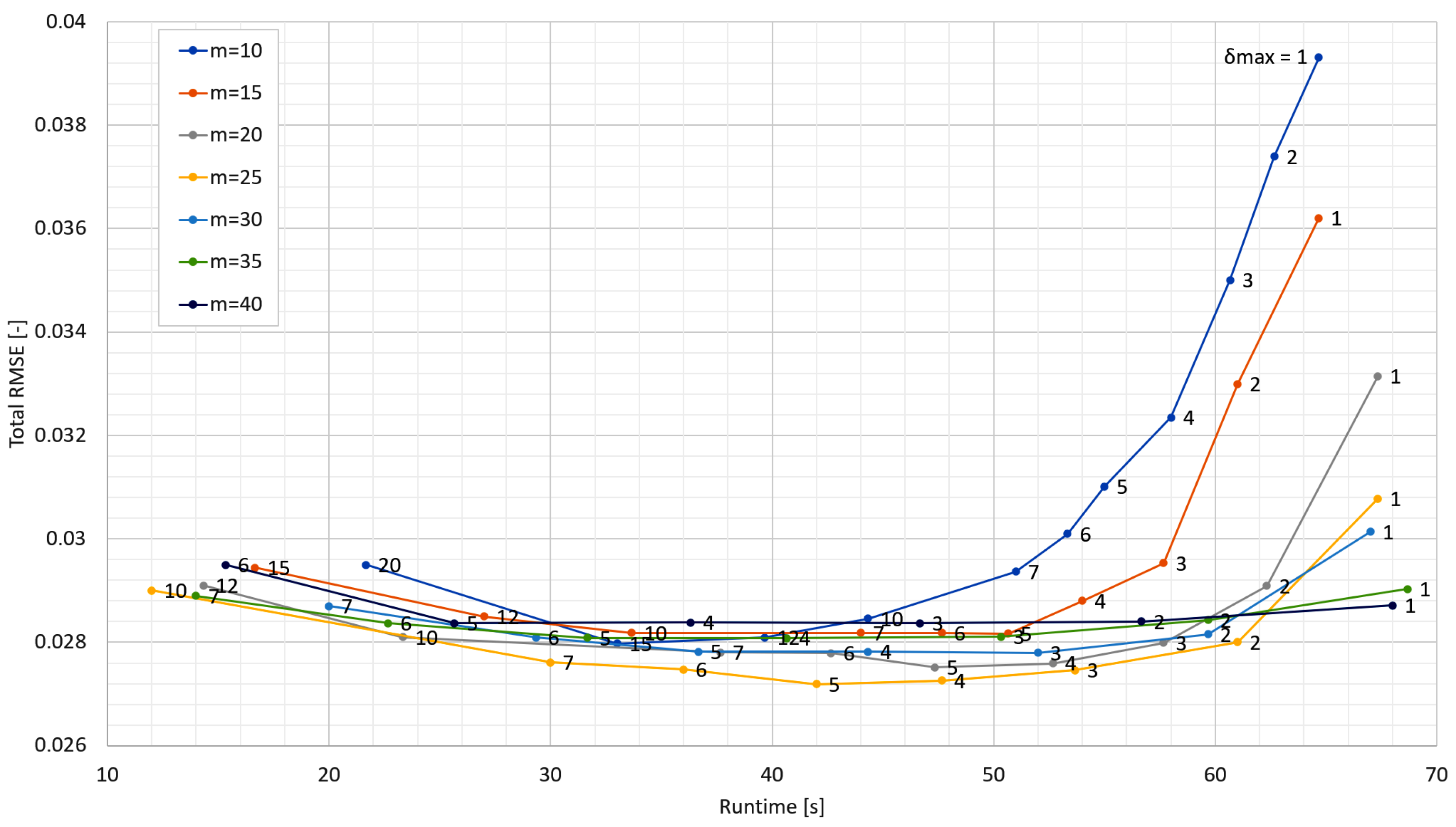
The parameters of the ARIMA(0,1,2) method were automatically determined by its auto.arima() function and the parameters of the ARIMA(8,1,6) method were determined by the recommended procedure using autocorrelation (ACF) and partial autocorrelation functions (PACF). The optimal parameter values used for all other methods were empirically located. For the RTDP method, this search is shown in Figure 3.

Table 1. Summary of the used parameter values of the compared methods.

Method	Parameters
ANN 1	$\eta =0.1$, 3 layers of 15 neurons each, $maxerror=0.01$
ANN 2	$\eta =0.1$, 3 layers of 15 neurons each, $maxerror=0.02$
ARIMA(0,1,2)	$p=0,d=1,q=2$
ARIMA(8,1,6)	$p=8,d=1,q=6$
KNN	$k=5,N=40$
RF	$ntree=13,mtry=19$
RTDP	${\delta }_{max}=5,m=25,N_p=30,N_{msp}=21$
XGB	$nrounds=22,\eta =0.23,minweight=20,maxdepth=1,\gamma =0$
Zeroth	$m=31,\tau =1,\epsilon =0.151$

then summarizes the parameter values of all methods used in the comparison.

5. Results

For all methods, the same number of previous samples (341) was used to predict of the following value. A time window of 340 samples was created and each method attempted to predict the value of the 341st sample. By sliding this time window over the entire power energy consumption time series, the waveform of the prediction error for each method was obtained.

The sampling rate of the predicted time series used is one sample per minute, so 340 samples represent a timespan of more than 5 hours. Over such a long period of time, power consumption trends should already be sufficiently evident. Of course, by using a longer time window, the predictions could be more accurate, but for the purposes of this comparison, this level of accuracy is sufficient.

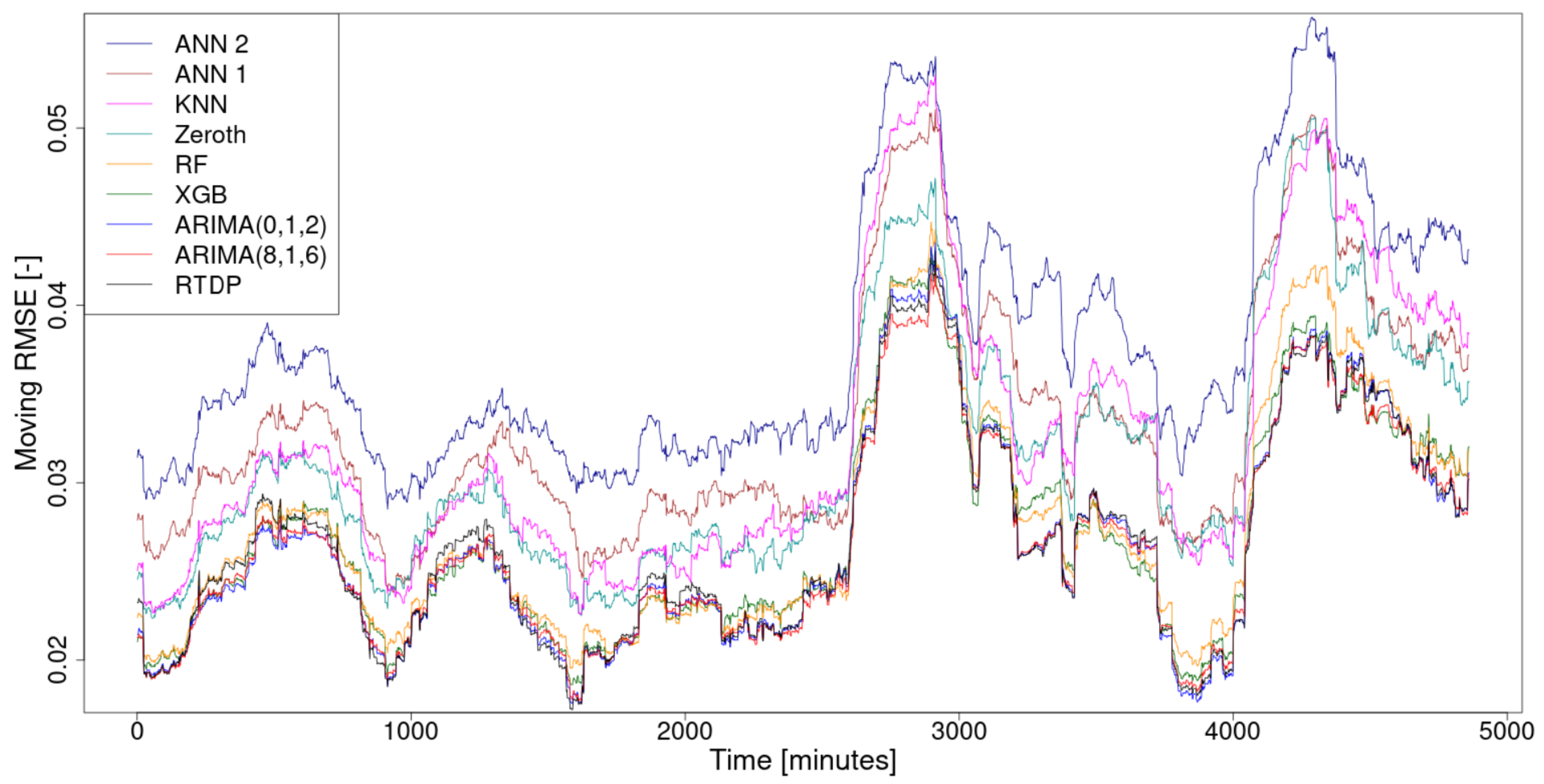
From the prediction error waveforms, the moving root mean square error (RMSE) waveforms, using a 300-sample-width moving window, were calculated for smoothing purposes and are shown in Figure 4. For each method, the overall RMSE was also calculated from this prediction error waveform and a sorted summary of these total RMSEs is given in

Table 2. The ranked results are summarized here by the total RMSE and also by the total runtime taken to calculate the predictions of the entire time series of supercomputer power consumption.

Method	Total RMSE [-]		Method	Total Run-Time [s]
RTDP	0.02719		Zeroth	23
ARIMA(8,1,6)	0.02722		RTDP	42
ARIMA(0,1,2)	0.02738		ARIMA(0,1,2)	58
XGB	0.02773		KNN	3240
RF	0.02836		XGB	4515
Zeroth	0.03231		ARIMA(8,1,6)	4714
KNN	0.03350		RF	7250
ANN 1	0.03414		ANN 2	25,501
ANN 2	0.03841		ANN 1	56,549

.

The prediction calculations of the machine-learning methods were conducted using the software R [9] package caret [10] and the calculation of the statistical method predictions was conducted using R package forecast [11].

In the case of the machine learning methods used (XGB, ANN, RF, KNN), the default resampling method of the caret software package was used to split the data into training and test sets. This is a bootstrapping method that builds a test set from 25% of the input data. Nonlinear and statistical methods (Zeroth, RTDP, ARIMA) do not use this partitioning in the training and test sets because they do not create a mathematical model that needs to be trained and then tested.

All calculations were performed on the same personal computer with an Intel Core i7-1065G7 processor (1.30–3.90 GHz) and 16 GB DDR4 RAM.

6. Conclusions and Future Work

In this paper, a new prediction method, named RTDP, was proposed. Using random time-delays patterns, this method tries to find important parts of the previous evolution of the time series and predicts its future evolution on this basis.

Its competitiveness was proved by comparing the accuracy of its prediction of the supercomputer infrastructure consumption time series with the accuracy of the prediction of the same time series when calculated with other commonly used prediction methods. The new RTDP method is based on the old and simple zeroth algorithm method and, thanks to the modifications, has gained in accuracy and lost a little in speed compared to the original method.

The comparison results, shown in Figure 4 and summarized in Table 2, show that the new RTDP method, when used to predict the evolution of supercomputer infrastructure consumption, was the most accurate and the second fastest. This is an excellent result, but to more comprehensively test this method, it will be necessary to perform this comparison on various types time series.

The development of the software package in which this method will be effectively implemented is another appropriate future work. The advantage of this method is its easy parallelizability, since calculations with individual $RTDP$s are independent of each other and can, therefore, run on different processor cores at the same time. It is reasonable to assume that the use of this feature will further speed up the method, which may also have an impact on its accuracy, as more $RTDP$s can be tried in the same amount of time.

References

- Bonaccorso, G. Machine Learning Algorithms; Packt Publishing Ltd.: Birmingham, UK, 2017. [Google Scholar]
- Brockwell, P.J.; Davis, R.A. Introduction to Time Series and Forecasting; Springer: Berlin/Heidelberg, Germany, 2016. [Google Scholar]
- IT4Innovations: Anselm, Salomon, DGX-2, and Barbora Supercomputer Clusters Located at IT4Innovations, National Supercomputing Center. Available online: https://www.it4i.cz/en (accessed on 31 August 2021).
- Kantz, H.; Schreiber, T. Nonlinear Time Series Analysis; Cambridge University Press: Cambridge, UK, 2003. [Google Scholar]
- Chen, T.; Guestrin, C. XGBoost: A Scalable Tree Boosting System. In Proceedings of the 22nd ACM SIGKDD International Conference on Knowledge Discovery and Data Mining, San Francisco, CA, USA, 13–17 August 2016; pp. 785–794. [Google Scholar]
- Tomčala, J. Predictability and Entropy of Supercomputer Infrastructure Consumption. In Chaos and Complex Systems, Springer Proceedings in Complexity; Stavrinides, S., Ozer, M., Eds.; Springer: Cham, Swizterland, 2020; pp. 59–66. [Google Scholar]
- Ho, T.K. Random decision forests. In Proceedings of the 3rd International Conference on Document Analysis and Recognition, Montreal, QC, Canada, 14–16 August 1995; pp. 278–282. [Google Scholar]
- Graupe, D. Principles Of Artificial Neural Networks: Basic Designs To Deep Learning; World Scientific: Singapore, 2019. [Google Scholar]
- R Core Team R: A Language and Environment for Statistical Computing. Available online: https://www.R-project.org (accessed on 31 August 2021).
- Kuhn, M. Caret: Classification and Regression Training. Available online: https://CRAN.R-project.org/package=caret (accessed on 31 August 2021).
- Hyndman, R.; Athanasopoulos, G.; Bergmeir, C.; Caceres, G.; Chhay, L.; O’Hara-Wild, M.; Petropoulos, F.; Razbash, S.; Wang, E.; Yasmeen, F. Forecast: Forecasting Functions for Time Series and Linear Models. Available online: https://pkg.robjhyndman.com/forecast (accessed on 31 August 2021).
Figure 1.
A simplified example of consumption aggregation. Energy consumption of 3 nodes running different jobs at the same time. Regular patterns merged together give a regular pattern, but the pattern is more complex, with a smaller degree of predictability.
Figure 2.
Power energy consumption time series. This is the normalized measured power from the infrastructure of the IT4Innovations [3] supercomputer. The measured timerange is from 1:00 p.m., 2 November to 9:00 p.m., 5 November 2017.
Figure 3.
Results of a series of predictions designed to empirically determine the optimal parameters of the RTDP method. The time series of power energy consumption, shown in Figure 2, was used to calculate these results. The numbers at the nodes represent the value of . The number of patterns and the number of the most successful patterns were set to and for the whole series. The RTDP method is (in this case) most accurate when the parameters and are set.
Figure 4.
Comparison of the prediction accuracy waveforms of the methods used with the new prediction method RTDP. The moving RMSE was calculated as the RMSE of a moving 300 samples wide window.