
Genetic Programming Guidance Control System for a Reentry Vehicle under Uncertainties


Intelligent Computational Engineering Laboratory (ICE-Lab), University of Strathclyde, Glasgow G11XJ, UK
*
Author to whom correspondence should be addressed.
Mathematics 2021, 9(16), 1868; https://doi.org/10.3390/math9161868
Submission received: 30 June 2021
/
Revised: 30 July 2021
/
Accepted: 3 August 2021
/
Published: 6 August 2021
(This article belongs to the Special Issue Evolutionary Algorithms in Engineering Design Optimization)
Abstract
:As technology improves, the complexity of controlled systems increases as well. Alongside it, these systems need to face new challenges, which are made available by this technology advancement. To overcome these challenges, the incorporation of AI into control systems is changing its status, from being just an experiment made in academia, towards a necessity. Several methods to perform this integration of AI into control systems have been considered in the past. In this work, an approach involving GP to produce, offline, a control law for a reentry vehicle in the presence of uncertainties on the environment and plant models is studied, implemented and tested. The results show the robustness of the proposed approach, which is capable of producing a control law of a complex nonlinear system in the presence of big uncertainties. This research aims to describe and analyze the effectiveness of a control approach to generate a nonlinear control law for a highly nonlinear system in an automated way. Such an approach would benefit the control practitioners by providing an alternative to classical control approaches, without having to rely on linearization techniques.
1. Introduction
Several decades after its formulation, and despite the great abundance of different control schemes and paradigms in the academic literature, the PID controller is still the most used control approach in industrial and real world applications. This is due to its simplicity, effectiveness and to the decades long active research. Nonetheless, it needs to be applied to linear or linearized models to work efficiently. This is particularly difficult in the aerospace domain, where the physics of the controlled plant and of the environment are defined by nonlinear models. To overcome the limitations of the PID controller and improve the performances and robustness of a control system, several control system design approaches have been proposed in the past, such as optimal control, adaptive control and robust control. However, all these different control system design approaches require accurate mathematical models and they are challenged by the nonlinear character of these models [1]. Moreover, as discussed by Haibin et al. [2] and Xu et al. [3], these complex systems have to meet stringent constraints on reliability, performances and robustness and the current control methods can only satisfy these constraints partially, usually by relying on simplified physical models. An in depth review of guidance control algorithms is presented by Chai et al. [4]. In their work, several guidance control algorithms are analyzed and divided into three main categories: Stability-theory based, optimisation-based and AI-based. Each of these three approaches present pros and cons which can be summarized as follows: Stability-theory based methods are characterized by a well defined mathematical formulation and proof of their stability; nonetheless, they present issues when dealing with uncertainties and when the controlled system models are not well defined. As for stability-theory based methods, also the optimisation-based methods’ robustness and stability are proved mathematically and they are flexible in the sense that they can be easily combined with other tools. However, they are computationally expensive, they have issues when dealing with constraints and nonlinearities and the reliability of the approaches devised to overcome these limitations, e.g., convexification, can be questioned. To overcome these issues and to fully exploit the available nonlinear models, AI could be used and integrated in classical control schemes. Despite the application of AI for control purposes is still in an early stage, it could greatly enhance the control capabilities and the robustness of classical control schemes. However, as pointed out in [4], they lack of mathematical proofs of reliability. A more in depth survey on some of the latest applications of AI in spacecraft guidance dynamics and control was produced by Izzo et al. [5] where the potential benefits of this research direction were assessed. A promising AI technique which can be used for control purposes is GP. GP is a CI technique belonging to the class of EAs. It was made known by Koza in 1992 [6] and it is capable of autonomously finding a mathematical input-output model from scratch to minimize/maximize a certain fitness function defined by the user. As other EAs, it starts from an initial population of random individuals and then evolves them using evolutionary operators such as crossover, mutation and selection until a termination condition is met. The evolution is guided by the principle of the evolution of the fittest and it proceeds by finding increasingly better individuals to solve the desired problem. In contrast to other EAs, in GP an individual is structured as a tree which represents a mathematical function. This clear representation of the models produced by GP is an advantage when compared to other ML techniques, like NNs, especially in a control context. In fact, to assess the reliability and robustness of a control scheme it is desirable to have the complete mathematical representation of it. This can be naturally achieved by GP while a NN produces a so called black-box model, where inputs are provided and outputs are produced but what is inside the model is not known to the user. The effectiveness of a GP based controller was discussed in [7], where it was shown that GP is capable of producing human-competitive results. In general, in a control context GP can be used to autonomously find a control law, starting from little or no knowledge of the control system, capable of performing the guidance or attitude control of a desired plant. It is not limited by the aforementioned nonlinearities and by being autonomous, it permits to avoid the cumbersome mathematical formulation of other control approaches. Hence, the aim of this work is to present a controller design approach based on GP applied to the reentry guidance control problem of the FESTIP-FSS5 RLV, considering the presence of uncertainties in the environment and plant models. The purpose of the presented control approach is to overcome the challenges related to the control of highly nonlinear systems. In particular, the proposed approach allows avoiding the use of linearization techniques that introduce modelization discrepancies and over simplified controllers that can fail in real conditions. This is particularly true for reentry applications, where the environment and aerodynamic models vary rapidly and modelization and control simplifications can result in system failures. To the best of the authors knowledge no application of GP to the guidance control of a reentry vehicle was found in the literature. The learning process is performed offline due to hardware limitations, but, as the hardware technologies improve, there will be the possibility to perform the process online in the future. A recent example of progress in this direction is represented by the work of Baeta et al. [8], where they proposed a framework to deploy GP using TensorFlow. If such an approach proves to be easily applicable to other GP applications, with improvements in the computational time of the same order of magnitude of those found in [8], it would represent a big step forward in the online usage of GP for control purposes. In fact, what was done so far in the literature consists in applying the GP offline to find a control law. On the other hand, if GP is used online, it is possible to define that control approach, IC [9].
The reminder of the paper is organized as follows: In Section 2 an overview of the different control approaches for reentry applications is provided; in Section 3 the theory behind GP and the particular GP algorithm employed in this work, the IGP, are presented along with a description of the IGP settings for this work. In Section 4 the chosen test case is described, while in Section 5 the obtained results are presented. Finally, in Section 6 the found conclusions and future work directions are discussed.
2. Related Work
Among the different control approaches employed for reentry applications, the most commonly used are MPC, Optimal Control and Sliding Mode Control. MPC is a control strategy akin to optimal control, in the sense that a finite-horizon optimization of the control variables is performed online while satisfying the imposed constraints. Luo et al. [10] used this technique to solve the attitude control problem of a reentry vehicle while considering the actuator dynamics and failure scenarios. A more recent approach involving MPC is proposed by Wang et al. [11], where they used a convex optimization with pseudospectral optimization inside an MPC framework, to solve a constrained rocket landing problem. Both these approaches proved to be successful, but in order to be applied, they must rely on simplified aerodynamic models or on the constraints convexification as done for the convex optimization approach. These restrictions are common to Optimal Control. In fact, the use of an optimizer, especially gradient based, inside a control framework is an issue if the models involved are nonlinear. Nonetheless, Optimal Control is widely used, both for ascent and reentry trajectory optimization. An example of that is represented by [12], where a pseudospectral optimal control approach is used to generate online the optimal guidance controls for a reentry vehicle in the presence of disturbances and constraints, but simplified aerodynamic models are used. A similar approach is used in [13], where a pseudospectral optimal control algorithm is combined with a sliding mode controller to take into account uncertainties, but also here a simplified aerodynamic model is used. Other usage of a sliding mode controller can be found in [14], where a sliding mode controller is used for the approach and landing phase of a reentry vehicle but simplified aerodynamic models are used and constraints are imposed only on the states variables. While in [15], an adaptive twisting sliding mode controller is used for the attitude tracking of an hypersonic reentry vehicle. Such an approach is not tested on a constrained problem and involves a cumbersome mathematical formulation.
All the aforementioned techniques can be considered “classical” approaches, in contrast to those based on AI. AI control approaches for reentry vehicles are more rare in the literature, but, as said above, the incorporation of AI in control systems is becoming more and more frequent. Few examples of these approaches are represented by the work done by Wu et al. [16] and Gao et al. [17]. In the former, a fuzzy logic-based controller is developed for the attitude control of the X-38 reentry vehicle; while on the latter, a Deep Reinforcement Learning approach is used for the reentry trajectory optimization of a reusable launch vehicle.
Among the various AI techniques employed, EAs are among the less employed. In particular to the best of the authors knowledge no control approach for a reentry vehicle involving GP was studied in the literature. For reentry applications, EAs are mostly used to find an optimal reentry trajectory, as it is done in [18,19,20]. Other uses of EAs in reentry applications can be found in [21], where GA is used to optimize the parameters of a sliding mode controller applied to the attitude control of a reentry vehicle. While, in [22] the evolutionary method Pigeon Inspired Optimization is combined with a Gauss Newton gradient based method to form a predictor-corrector guidance algorithm. The goal of this guidance scheme is to use the EA to generate an initial condition for the gradient-based method to solve the entry guidance problem.
3. Genetic Programming for Control
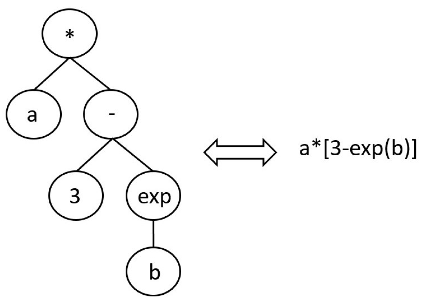
Genetic Programming (GP) is a Computational Intelligence (CI) technique pertaining to the class of Evolutionary Algorithms (EAs) made known by Koza in 1992 [6]. As other EAs, GP consists in evolving a program from an initial population of randomly generated programs, to minimize/maximize a defined fitness function. Such evolution is performed according to the defined crossover, mutation and selection operators, in order to steer the evolution of the population in the desired direction and avoid local minima. Compared to other EAs, in GP the individuals are shaped as trees which corresponds to symbolic mathematical equations as depicted in Figure 1, where a, b and 3 are called terminal nodes, and a and b are the input variables. The other nodes in the GP tree corresponds to the primitive functions provided by the user and employed by the GP algorithm to build programs autonomously.
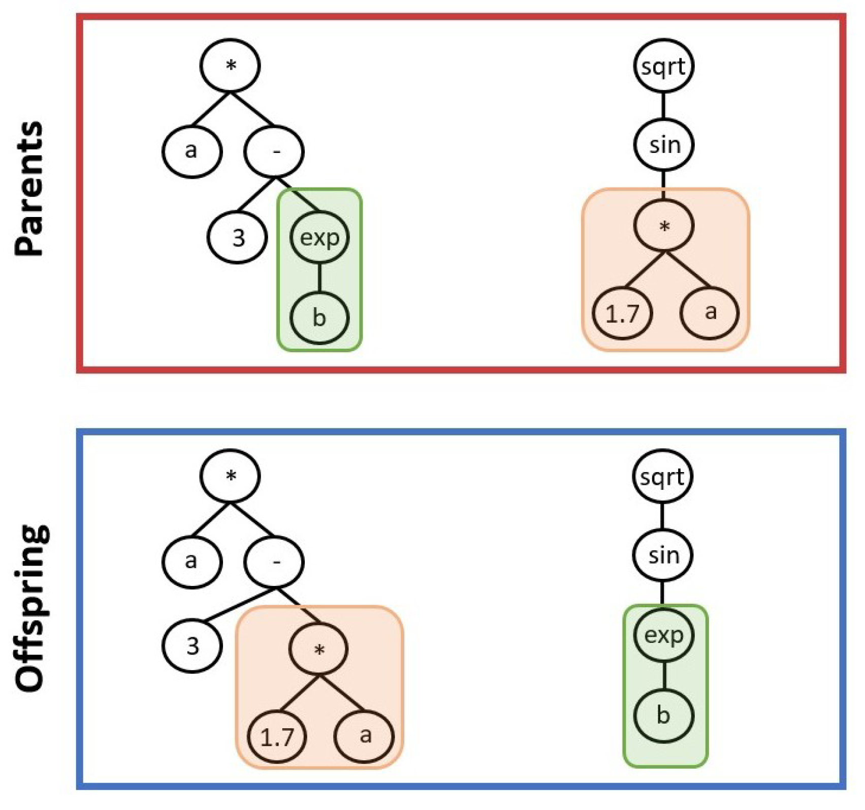
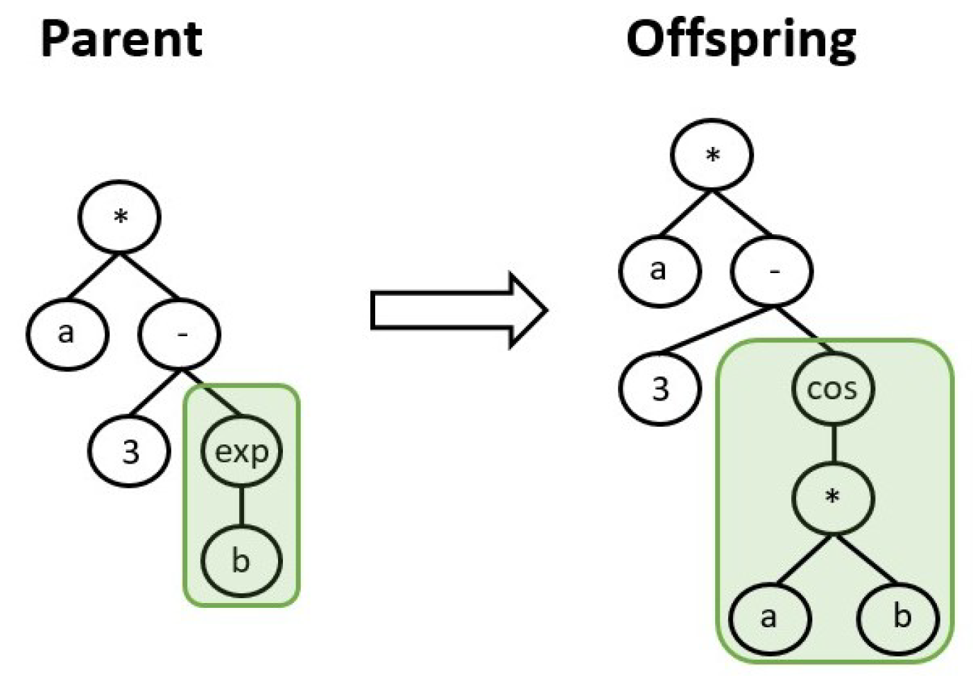
About the evolutionary operators, crossover consists in an exchange of genes between two parents individuals to produce other two individuals as offspring. Looking at Figure 2, two genes highlighted by the green and orange boxes are exchanged between the parents to form the offspring. Regarding the mutation operation, a randomly chosen gene of a chosen individual is randomly mutated to generate a new offspring, as depicted in Figure 3. Several different types of the crossover and mutation operators were devised in the past decades and which one to choose is highly dependant on the particular problem to solve. Since it is not the aim of this work to provide a comprehensive description of the peculiarities of the GP algorithm, the reader is referred to [6] for more details.
Regarding the control applications of GP, several examples can be found in the literature. In [23] a multi-objective GP is used to evolve controllers for a UAV allowing it to navigate towards a radar source. In [24] an adapted GP approach is used to generate the control law for a UAV which provides recovery onto a ship considering real world disturbances and uncertainties. Other control approaches involving GP are represented by [25] where GP is used to generate a control Lyapunov function and the modes of a switched state feedback controller; while in [26] GP is used to generate a PID based controller. All these approaches involving GP for control applications cannot be considered IC. In fact, the GP evaluation is done offline and no online learning is present. An example of GP used in an IC framework is represented by the work of Chiang [27] where the control law for a small robot is produced online using GP, with the aim of moving the robot in an environment filled with obstacles. A similar approach was used in [28], where a guidance controller for a Goddard rocket is designed online to cope with different kinds of uncertainties. In contrast to this last example, the work presented here aims to generate a control law for a much more complex and nonlinear system, also considering more severe uncertainties. This results in a longer computational time, hence the impossibility to use it online with the current hardware technology. In fact, to generate the control law online successfully, the considered plant must be very simple in order to perform the evolutionary process in a useful time interval.
As opposed to all these examples, the approach proposed in this work is developed considering a more complex plant model and uncertainties are also taken into account. In fact, the proposed control approach takes into account the nonlinearities present in the models of the vehicle dynamics, the aerodynamics and the environment while uncertainties are applied to the environment and aerodynamic models. Moreover, to the best of the authors’ knowledge this is the first application of GP to perform guidance control of the reentry trajectory of an RLV.
The work produced in [28] was later used as a foundation to design the Hybrid GP-NN controller presented in [29]. In this control system, the GP was used offline to generate a control law that was later optimized online by a NN. The approach to generate offline the GP control law is the same used in this work, with the following differences: (1) A different more challenging application is considered, (2) more severe uncertainties are applied and (3) a more thorough analysis of the GP performances is conducted than the one performed in [29].
3.1. Inclusive Genetic Programming
The particular GP algorithm used in this work is the Inclusive Genetic Programming (IGP), which was originally presented in [29] and later analyzed in [30]. IGP was developed in Python 3 relying on the open source library DEAP [31]. IGP was designed to promote an maintain the population’s diversity throughout the evolutionary process, so to avoid losing big individuals due to bloat control operators. In fact, it was observed in [29] that bigger individuals are capable of handling the nonlinearities of the treated problem better than smaller individuals. Therefore, to maintain the population’s diversity and hence also preserve big individuals, three main features were inserted in the GP algorithm so to make what is now called the IGP. These features are: (1) A niches creation mechanism; (2) the Inclusive Reproduction and (3) the Inclusive Tournament. The creation of the niches implies that IGP belongs to the class of niching method. Niching methods are among the various methods used to tackle the diversity issue in GP. In contrast to standard niches approaches, the IGP makes use of the niches in a different manner. In fact, in the IGP the niches are used to make sure that the majority of the individuals are considered during the evolutionary process and that a flow of genes is established between the different niches. While in standard niching methods, the niches are separated and are used to find different local optima in a multimodal optimization, by parallel evolving the different niches towards different optima [32].
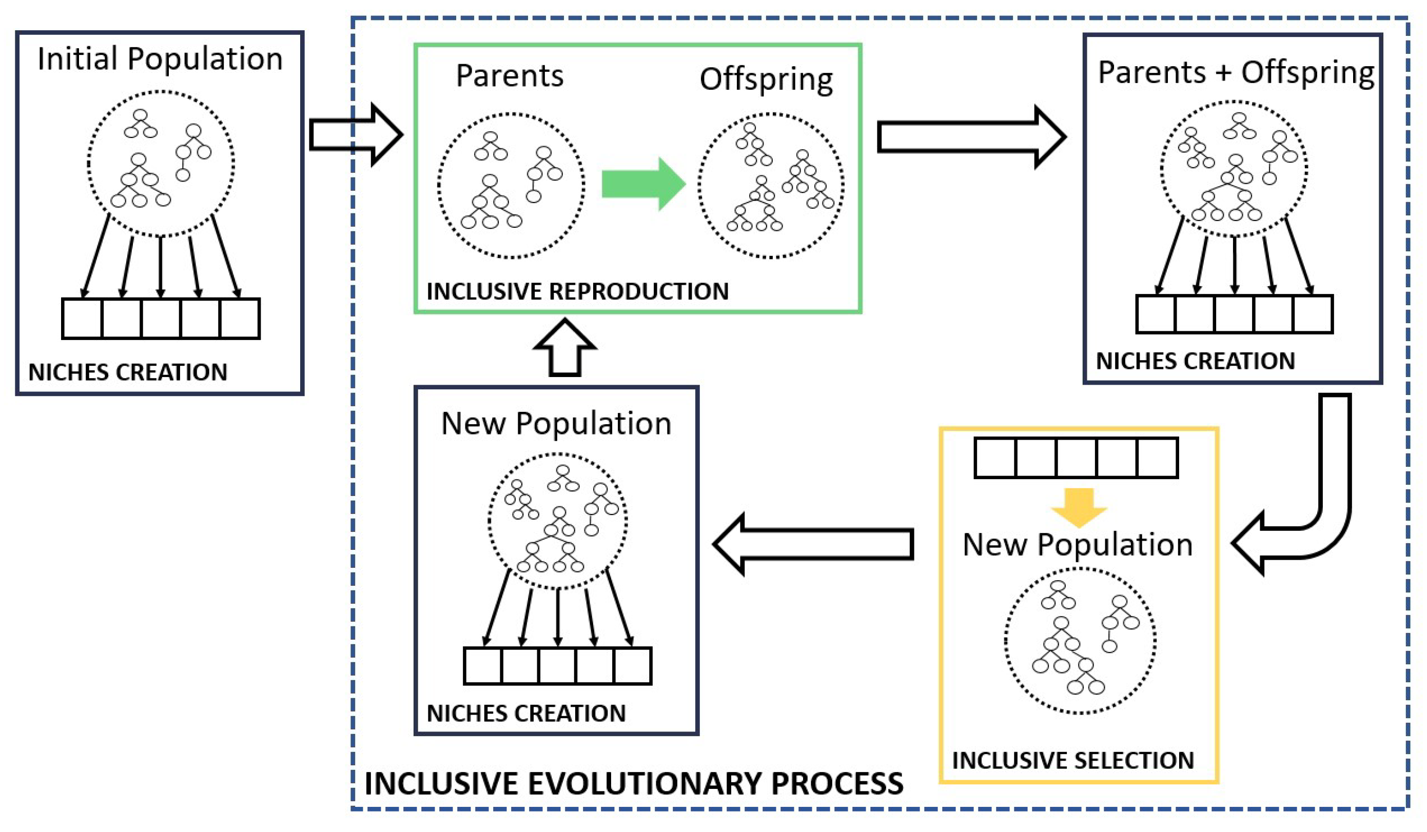
The whole Inclusive Evolutionary Process is based on the evolutionary strategy [33] and it is schematized in Figure 4. The process starts with an initial population which is subdivided into niches. Then the Inclusive Reproduction is performed, offspring is produced and the total of the individuals (parents+offspring) is subdivided into niches. These new niches are used to select individuals from the new population, which is again subdivided into niches and the process starts again.
Regarding the niches creation mechanism, the individuals in the IGP populations are divided into niches according to their genotypic diversity, which is the number of nodes inside each individual, i.e., their length. Each niche will cover a lengths interval, defined by the maximum and minimum lengths of the individuals in the population, and the number of niches. This way, each niche will be placed between the extremes of each interval and these extremes are evenly spaced between the maximum and minimum length of the individuals in the population. For example, if the maximum length is 30, the minimum is 5 and 5 niches are created, the lengths intervals that the niches will cover will be [5, 11.25], [11.25, 17.5], [17.5, 23.75], [23.75, 30]. So the first niche will contain those individuals with a length between 5 and 11.25 and so on. The number of niches to create is decided by the user and this number is kept constant throughout the evolutionary process. Nonetheless, the lengths intervals that they cover will change during the evolution since the maximum and minimum lengths of the individuals in the population will change. This allows for a shifting of the individuals between contiguous niches, helping to maintain diversity.
About the Inclusive Reproduction, it is designed to consider all the niches during the mating process. To perform crossover, two niches are selected from a list of available niches which is updated as the process goes on. Such an update consists in removing the selected niches and when all of them are selected, the list of available niches is reset to its initial state. Regarding the two selected niches, the best performing individual is selected from the first niche and a random one is selected from the second, this to consider the best performing individuals but also to avoid losing diversity. When mutation is selected, a niche is selected from the list of the available niches and such list is updated as said above. Then a random individual is chosen from the list. The individual is chosen randomly since applying mutation to the best performing ones does not guarantee an improvement. While, when 1:1 reproduction is selected, the best individuals is passed unaltered to the offspring. These selection criteria are summarized in Table 1.
Finally, the Inclusive Tournament consists in applying a Double Tournament [34] to all the niches sequentially, where each niche can be considered at most t times, where t is the number of individuals inside them. This is done to reduce the probability of having clones in the population. More on the Inclusive Reproduction and Selection can be found in [30]. Finally, other two peculiarities of the IGP in comparison to other GP formulations are its ability to handle constraints and the fact that is set to evolve more than one GP tree simultaneously.
3.2. Inclusive Genetic Programming Settings
The ability of the IGP to handle constraints and to evolve more than one GP tree at the same time, makes it particularly suited to solve control problems. In fact, the possibility to evolve more than one GP tree at the same time, allows to solve a control problem with more than one control parameter, which is often the case for most applications.
To produce the results presented in Section 5, the IGP was set as in Table 1, and two GP trees are evolved simultaneously, one for each control parameter of the considered problem. These will referred as -individual and -individual from this point onward.
Regarding the fitness functions, they are designed to solve the considered problem: The vehicle’s final position must be inside the FAC box, as described in Section 4, while satisfying the imposed constraints on normal acceleration, dynamic pressure and heat rate. To reach this goal, the fitness functions were implemented as in Equation (1). The evolutionary strategy on which the IGP was built, is such that first it favors those individuals that minimize and satisfy the constraints violation. So it first tries to get , then it favors those individuals with a better, i.e., lower, value of the fitness , which tells how close the final position is to the desired one. RMSE in Equation (1) is the Root Mean Square Error.
In Equation (1), is an array composed as in Equation (2) by the values of the IAE between the reference states and the actual ones evaluated on the last 50 points of the trajectory, as in Equation (3), where is evaluated as in Equation (4). For more details on the states and the whole test case, see Section 4.
The integrals inside were not evaluated on the whole trajectory but only on its last 50 points. This was done to encode in the fitness function the instruction for the GP to find a control law that produces a trajectory similar to the reference one in the last part, but it leaves it freedom on the rest of it, except for the constraints satisfaction. This way, the GP has more freedom to find a control law that satisfies the constraints but does not necessarily needs to track exactly the reference trajectory, which might be impossible due to the presence of uncertainties. In fact, the trajectory is considered successful if the constraints are satisfied and the vehicle’s final position is inside the FAC box. This last information is encoded in the array of Equation (1) which is composed as in Equation (5) and where the errors are evaluated as in Equation (4).
The array contains the errors between the final value of h, and and their final value of reference. The different way to evaluate the errors on the states, as shown in Equation (4), is done to balance their values since the errors on and tends to be much smaller that those of the other states. For the same reason, was divided by 10 in Equation (5). Moreover, to make the FAC requirement more important than the minimization of the tracking errors, in Equation (1) was multiplied by 1000 and was divided by 100. This combination of scaling factors is an heuristic that was defined experimentally, so it could be improved. Nonetheless, it is important since the magnitude of the different errors and IAEs varies of several orders of magnitude.
is implemented in a more straightforward way. CV in Equation (1) represents an array composed by the constraints violations measured during the evaluation of the trajectory. The constraints violation is evaluated as the error between the constrained quantity and its maximum or minimum value. If such an array is empty, meaning that the trajectory satisfies all the constraints, is set to 0.
About the other features listed in Table 1, the mutation and crossover rates are changed dynamically during the evolutionary process. The mutation rate starts at 0.7 and it is decreased by 0.01 at every generation while the crossover rate starts at 0.2 and it is increased by 0.01 at every generation, until the mutation rate becomes 0.35 and the crossover rate 0.65. This change is done if at least one individual with is found at the current generation. The rationale behind this approach is that exploration is favored at the beginning of the evolutionary process and until at least one individual that satisfies the imposed constraints is found. While, exploitation is favored towards the end of the evolutionary process to find better individuals. Then, limit height and size are two parameters used by the bloat control operator, which is the same implemented in the DEAP library but modified to take into account individuals composed by multiple GP trees. Moreover, the crossover and mutation operations, which are the same of the DEAP library, are modified to take into account individuals composed by multiple GP trees. Four different mutation mechanisms were used as listed in Table 1 and the probability of them being selected when mutation is applied is reported in the brackets near them. Finally, about the operations listed in the primitive set, is a ternary addition, , and are protected square root, logarithm and exponential to avoid numerical errors.
4. Test Case
To test the proposed control approach, a reentry mission of the FESTIP-FSS5 RLV is simulated. This vehicle was chosen since by being a spaceplane, it possess more control capabilities than a classical rocket and its guidance control during the reentry phase is particularly challenging due to the rapidly varying aerodynamic forces. The model of the vehicle, as well with the aerodynamic and atmospheric models, were taken from [35] and it is characterized by a lifting body and an aerospike engine. For the considered mission, two control parameters were considered, the angle of attack and the bank angle . The aerodynamics models are composed by two lookup tables that give the values of and as a function of the Mach and angle of attack. These data were obtained from experimental data, hence they form a nonlinear model. The aerodynamic data were smoothed with the CSG approach described in [36]. The atmospheric model is the USSA-1962 model. Regarding the mission, its details were taken from [37] and they are summarized in Table 2.
As described in [37], the final conditions corresponds to the target FAC box so to have an horizontal landing at the Space Shuttle Landing Facility at the NASA Kennedy Space Center. The FAC is defined by the final values of h, , and their respective tolerances. A trajectory was considered successful if the final position of the vehicle was inside the FAC box.
Regarding the constraints in Table 2, the one on the dynamic pressure q comes from the original formulation of the problem from [35]. The constraint on the normal acceleration was increased from 15 to 25 , to correspond to a load factor of about 2.5 g’s. This choice was made to be more in line with the load factor constraint imposed in [37], since the aim was to fly a similar trajectory. The heat rate constraint was taken from [38] and was modeled as in Equation (6)
where and . This heat rate model was chosen since no data of the FESTIP-FSS5 vehicle were available, and as reported in [38], the chosen heat rate model is a conservative approach. For more details on the heat rate model, please refer to [38].
4.1. Reference Trajectory
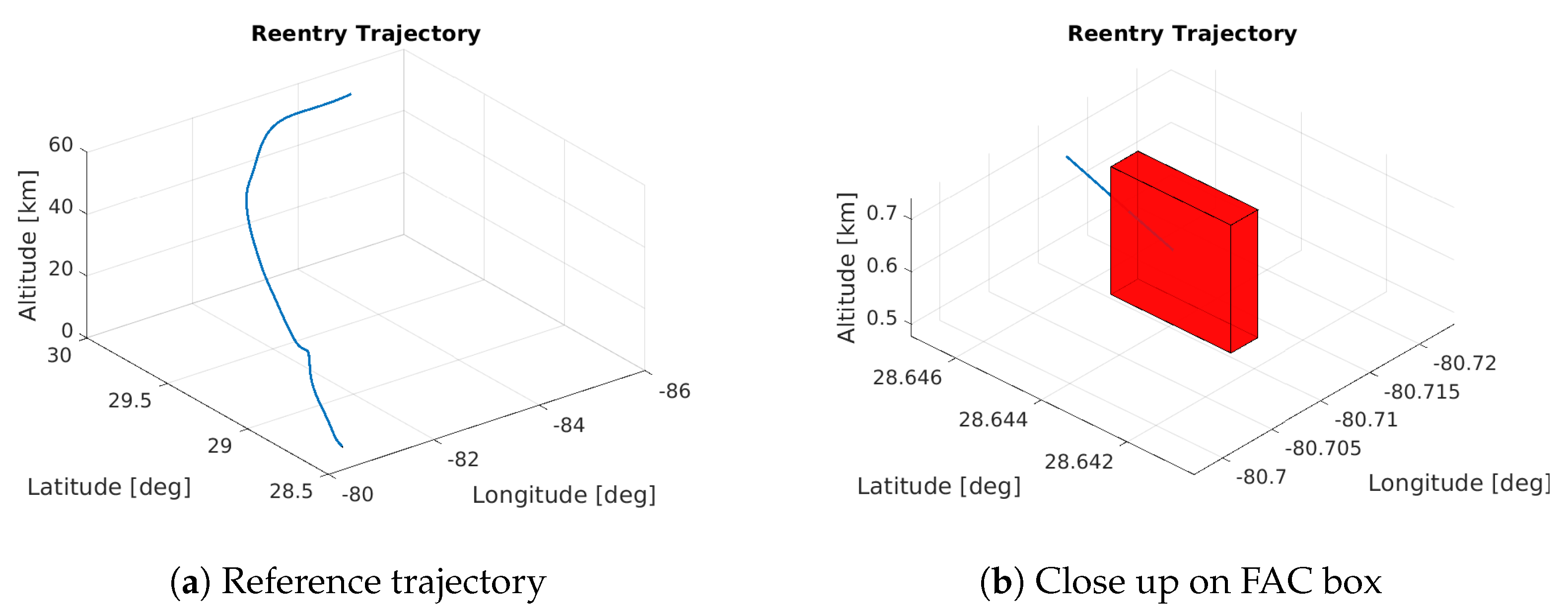
The trajectory used as reference for the controller was obtained by solving an optimal control problem using a Multiple-Shooting transcription. The initial guess research for the Multiple-Shooting was performed with the approach presented in [36]. The objective function was set to minimize the difference between the actual final position and the desired one while satisfying the constraints in Table 2. The obtained reference trajectory is shown in Figure 5.
4.2. Uncertainty Model
The control mission is simulated by inserting uncertainties into the aerodynamic and atmospheric models. The formulation of the uncertainties was taken from [39]. According to these models, the uncertainties were formulated by creating different sets of interpolating surfaces which were applied to the atmospheric and aerodynamic models to make them vary within a certain range from their unperturbed values, as in Equation (7).
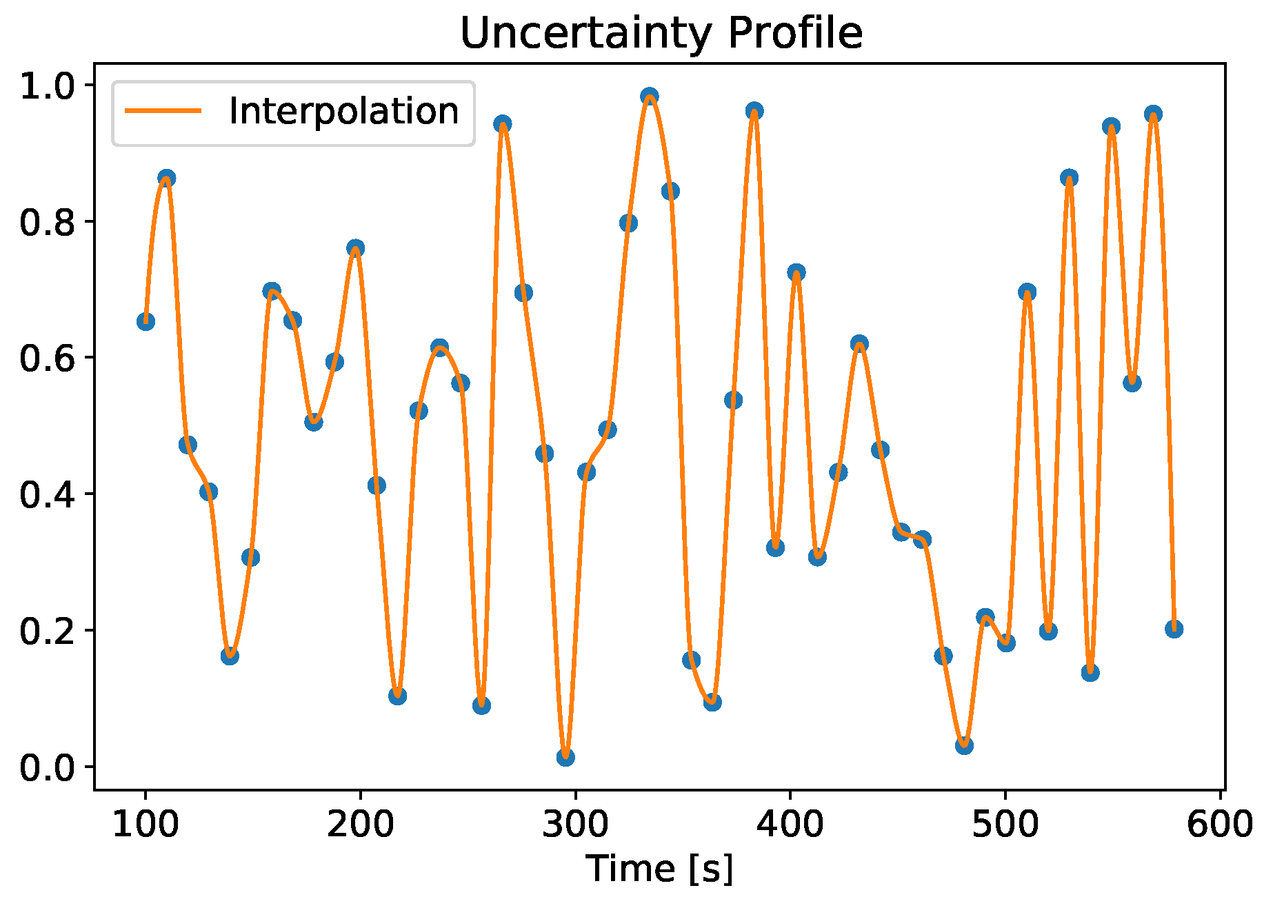
In Equation (7), is the nominal value of the quantity on which the uncertainty is applied, is the uncertainty bounding parameter and r is a random parameter varying in the interval [0, 1]. Using Equation (7), the quantity nominal value is randomly varied in the interval . The random value r is picked from an uncertainty profile obtained by interpolating 50 points randomly generated and uniformly distributed as in Figure 6. Here, the time starts at 100 s since the uncertainties were inserted at 100 s, as explained in Section 5.
In this work, three interpolating surfaces, for the pressure, temperature and aerodynamics, were created for each different uncertainty scenario in the uncertainty set. Each uncertainty set is composed of 20 uncertainty scenarios and 11 uncertainty sets were created in this work, for a total of 220 uncertainty scenarios. According to what was done in [39], three parameters were evaluated, one for each perturbed quantity. The reference values of the upper and lower bounds, and the other quantities used to evaluate the parameters are the same as in [39], and are summarized in Table 3, with the exception of , and which were changed according to the considered problem.
5. Results
All the results in this work were obtained on a laptop with 16 GB of RAM and an Intel® Core™ i7-8750H CPU @ 2.20GHz × 12 threads and multiprocessing was used. The code was developed in Python 3 and it is open source and can be found at https://github.com/strath-ace/smart-ml (Last accessed on 4 April 2021).
The methodology to test the proposed control approach was structured so to prove the ability of GP to find an adequate control law in the presence of various levels of uncertainties. These uncertainties were applied after 100 s from the start of the mission. After the applications of the uncertainties, the trajectory was flown using the reference control values until one of the states went outside the range of from its reference value. When that happened, the GP evaluation was started. This was done to simulate the scenario where the system has to adapt during flight to changes in the environment and plant models.
To define the level of uncertainty, the parameter in Equation (7) was varied. As explained in Section 4, three parameters were used, one for each perturbed quantity. These parameters were varied by increasing the boundaries used to evaluate them, by in each different simulation. The starting values are those listed in Table 3 and they correspond to those used in Simulation 0 in Table 4. Then they were increased by in Simulation 1, in Simulation 2 and so on. These settings are summarized in Table 4. For each simulation, a different uncertainty set was produced which was composed by 20 different uncertainty profiles, where an example of uncertainty profile is shown in Figure 6. Therefore, 20 GP runs were performed for each different simulation and a total of 11 different simulations was performed, so up to increment in the bounds values. This lead to a total of 220 GP runs performed. Twenty uncertainty profiles were produced for each uncertainty set so to avoid having too big computational times and a total of 11 simulations was performed, since it was physically meaningless to have too big uncertainties.
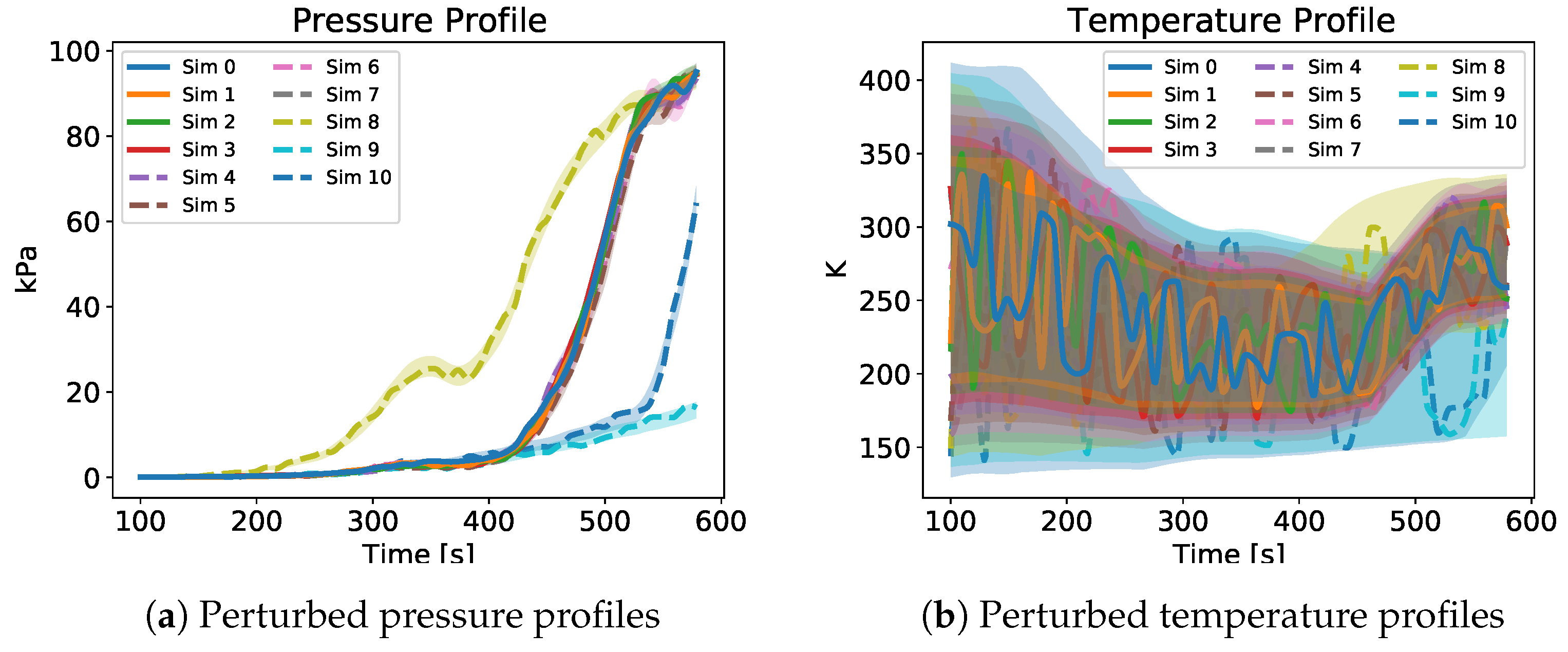
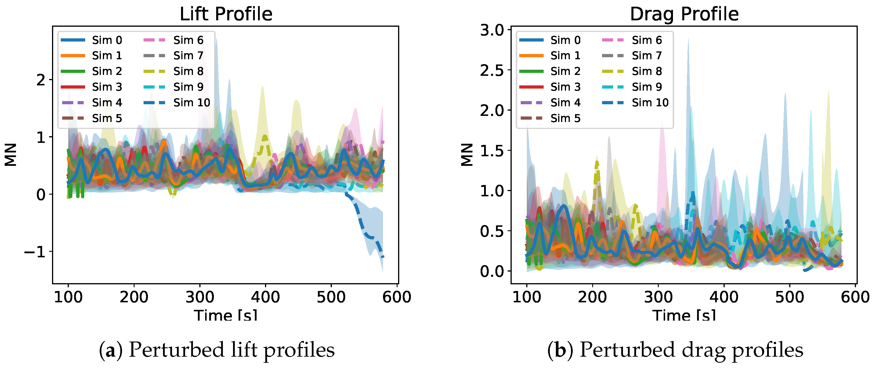
Figure 7 and Figure 8 show a qualitative depiction of some of the profiles of the perturbed quantities. The profiles on these pictures come from the first GP run of each simulation. The continuous lines represent the successful cases while the dashed lines the unsuccessful ones. The shaded ares represent the regions contained between the uncertainty bounds and in which the perturbed quantities could have varied when applying the disturbance profiles like the one in Figure 6. As already said, Figure 7 and Figure 8 are purely qualitative but they give an idea of the magnitude of the applied uncertainties. In particular, in Figure 7b the progressive increase of the uncertainty bounds from one simulation to the next is clearly visible.
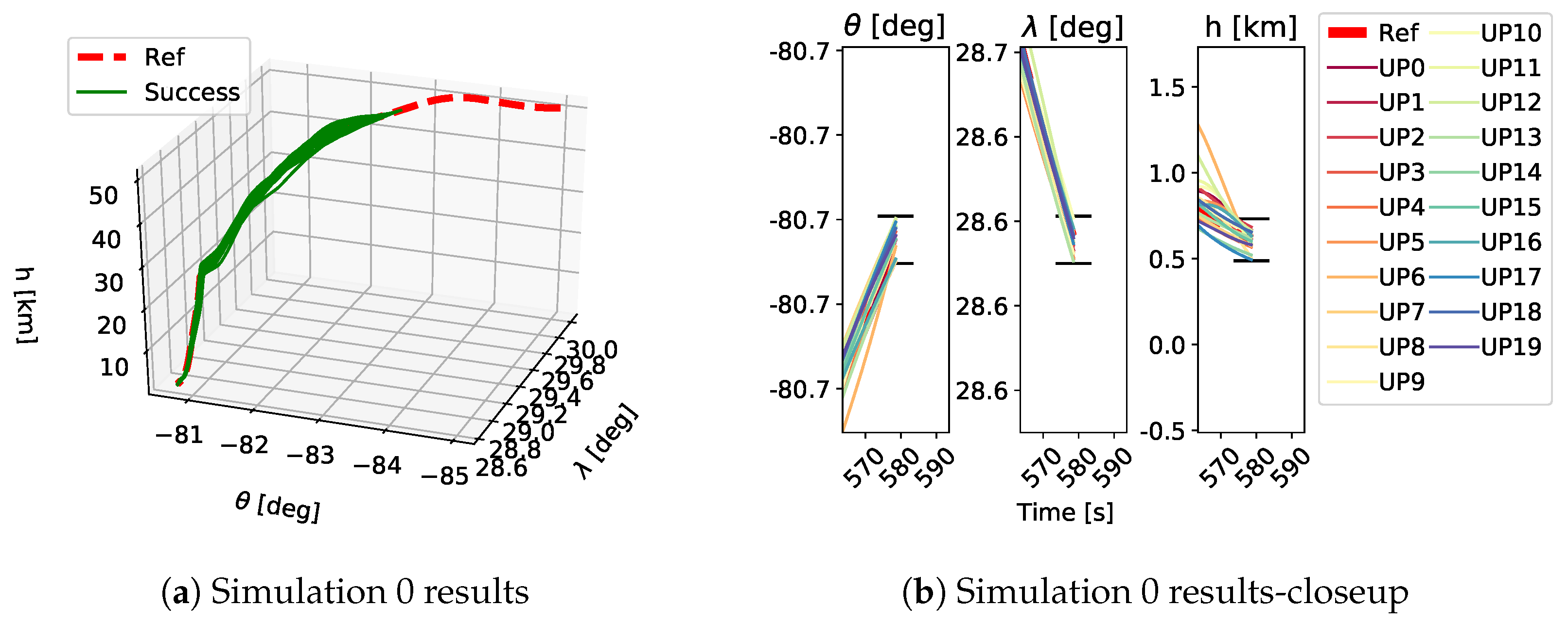
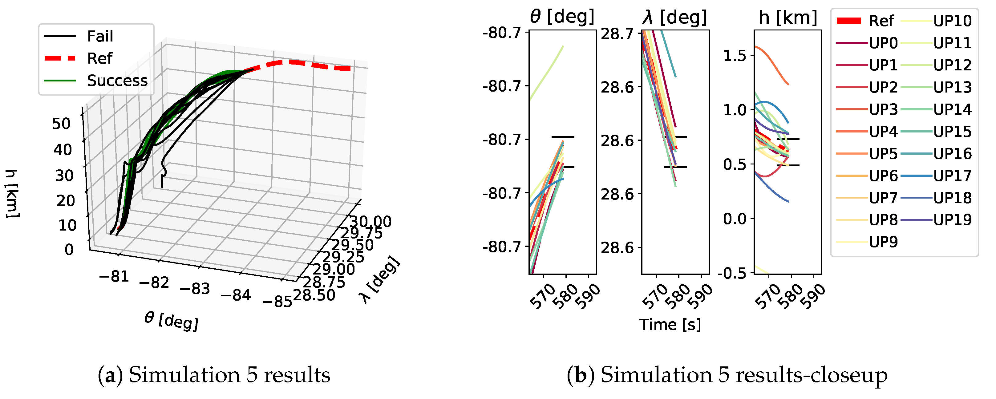
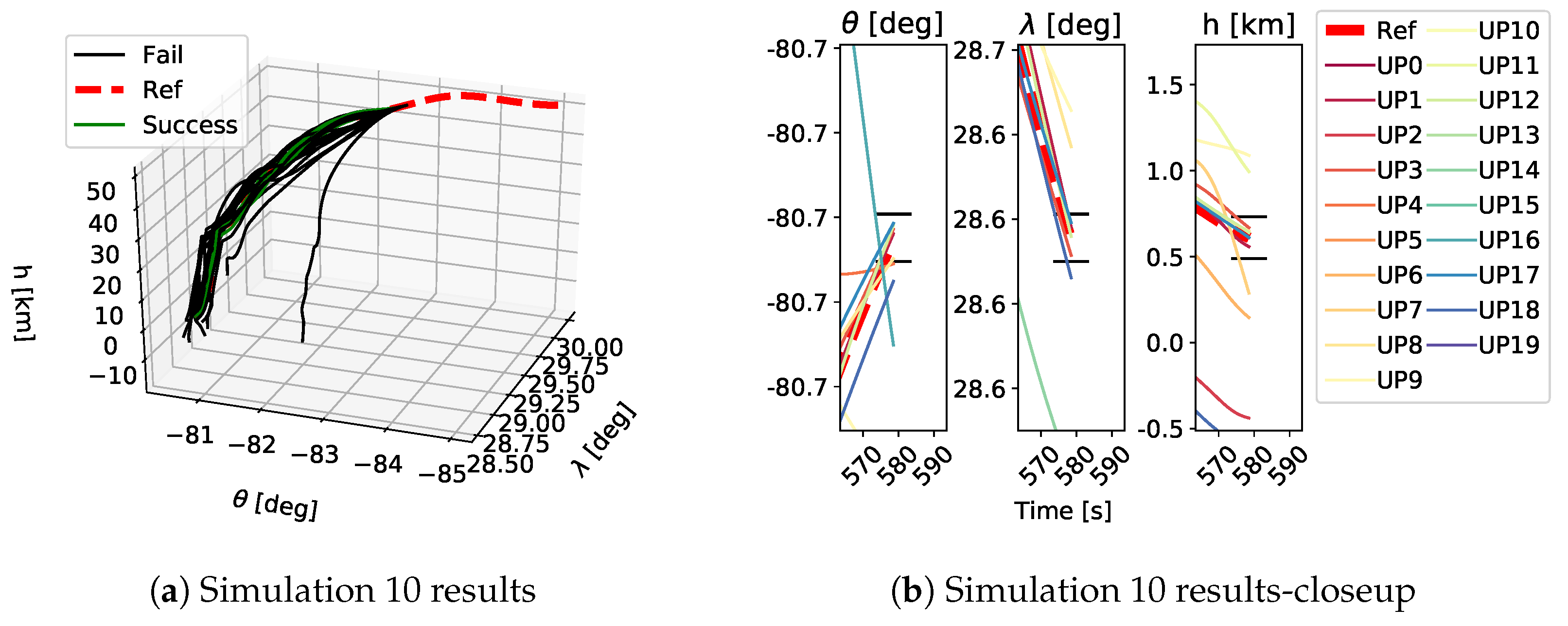
As shown in Table 1, each GP simulation was run until a successful trajectory was found or it was stopped after 150 generations. As stated above, a trajectory was considered successful if the final position of the vehicle was within the FAC box and the constraints were satisfied for the whole trajectory. A qualitative example of the performed trajectories is depicted in Figure 9, Figure 10 and Figure 11. Here the performed trajectories of the 20 GP runs for Simulations 0, 5 and 10 are shown. In plots Figure 9a–Figure 11a the full reentry trajectories are plotted in terms of altitude h, longitude and latitude , where the red dashed line is the reference trajectory, the green lines are the successful trajectories and the black lines are the failed trajectories. These trajectories show the three-dimensional path of the vehicle during the reentry phase and it is clear how, when increasing the magnitude of the applied uncertainties, the vehicle tends to stray from the reference trajectory. The plots Figure 9b–Figure 11b show a closeup on the final part of the trajectory to highlight the FAC box and how close the obtained trajectories got to it. The FAC box is projected onto its components , and h and it is represented by the black horizontal lines. Despite being a qualitative depiction, it can be seen from Figure 9, Figure 10 and Figure 11 how the performed trajectories deviates more and more from the reference as the magnitude of the applied uncertainties increases.
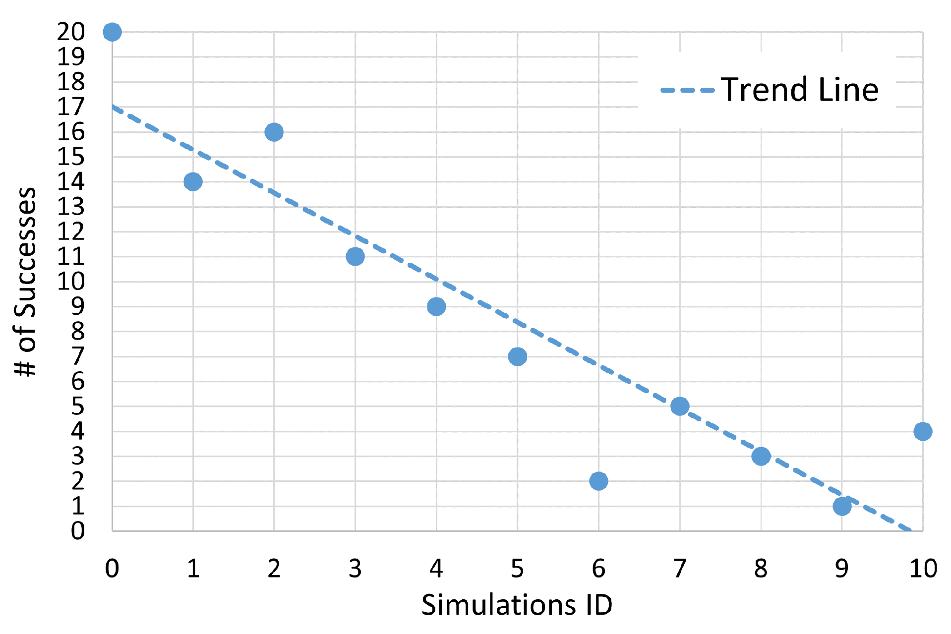
For a more quantitative point of view, the number of successes for each simulation is shown in Figure 12. Here, it is clear that with the reference values of the uncertainty bounds, the GP is able to find a successful control law of the times and this success rate tends to decrease as the uncertainty bounds increase, as expected. Three cases go against this trend, namely Simulations 1, 6 and 10. This is probably due to the fact that 20 GP runs for each simulation are not enough to constitute a statistically significant sample. Therefore by increasing the number of GP runs for each simulation, a more accurate trend could be achieved. Nonetheless, the obtained results are useful to understand the extent of the capabilities of the GP. In fact, even with an increase of of the uncertainty bounds, the GP is capable of finding four good control laws.
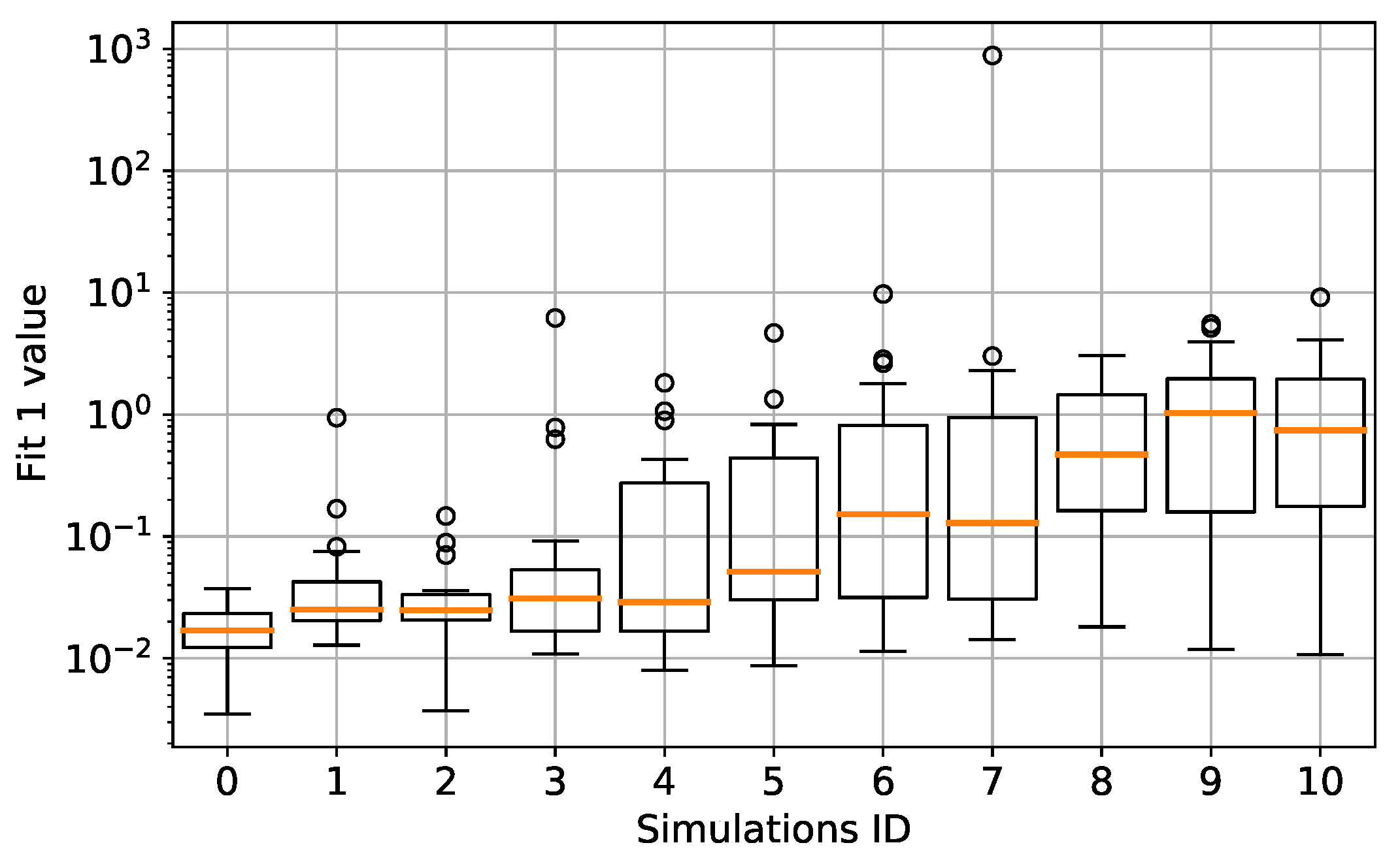
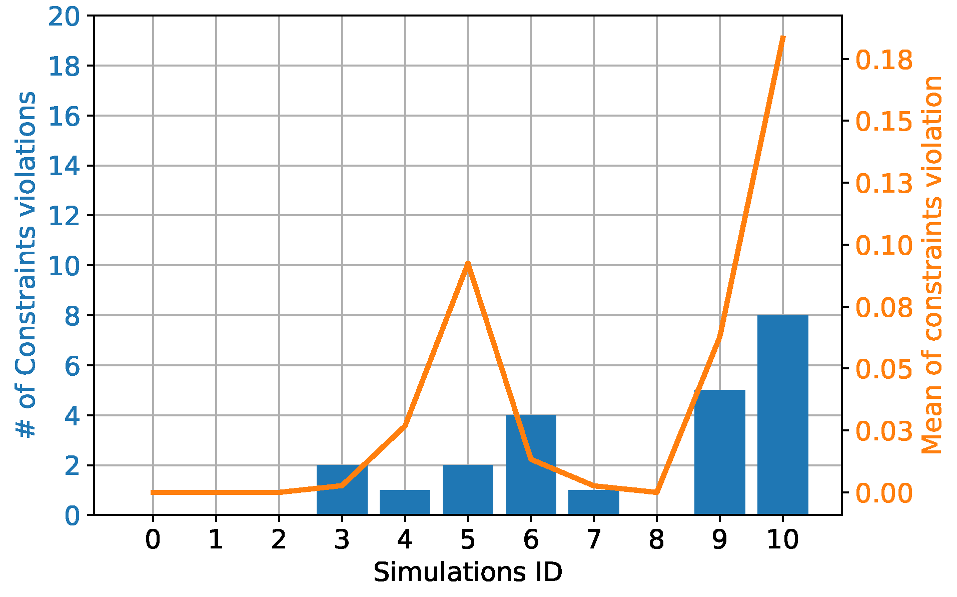
This success trend is also highlighted in Figure 13, where the median and standard deviation values of the first fitness function are shown. Here the median fitness value increases as the uncertainty bounds increase and the smaller value is found at Simulation 0. Moreover, the standard deviation also increases as the uncertainty bounds increase, as expected. A different perspective of the same phenomenon is observable in Figure 14. Here the number and magnitude of the constraints violation for each simulation are shown. The bar plots show the number of GP runs whose best individual violated the constraints, for each simulation. For example, in Simulation 3, two individuals out of 20 violated the constraints. The line plot refers to the mean value of the constraints violation for each simulation. These results show an increase in the GP runs that violated the constraints as the uncertainty bounds increase. Concurrently, the magnitude of constraints violation also increases as the uncertainty bounds increases. Nonetheless, as said before, the number of GP runs for each simulation was not enough to have a proper statistical sample.
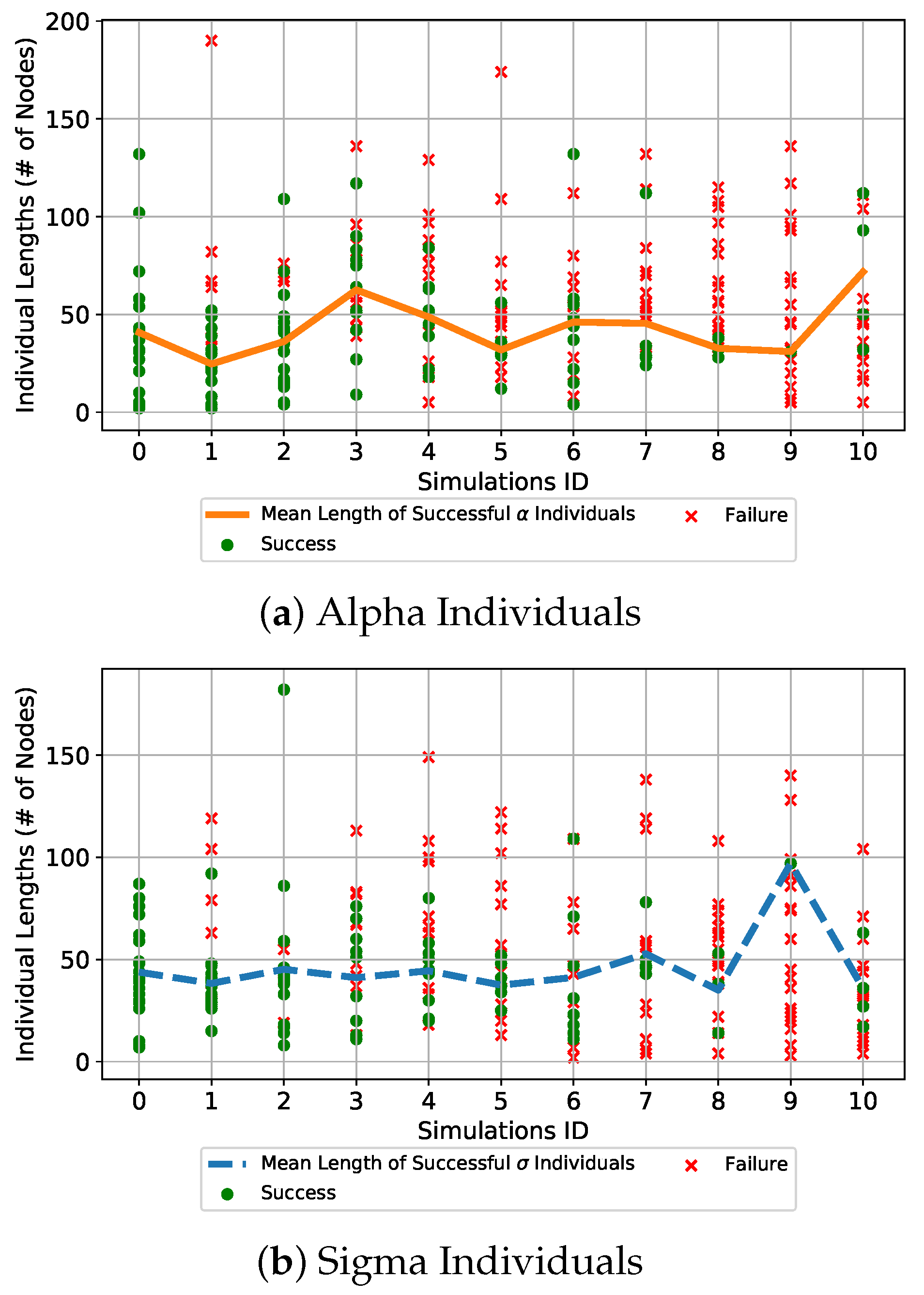
To have a greater insight into the produced individuals from a genotypic perspective, the lengths of the individuals were analyzed. In Figure 15, the lengths of the successful and unsuccessful individuals for each simulation are plotted. As said in Section 3, two individuals were simultaneously produced in each GP run, since two control parameters had to be found. The lengths of the -individuals are plotted in Figure 15a and those of the -individuals are depicted in Figure 15b. These lengths are represented by the green dots for the successful individuals and the red crosses for the unsuccessful ones. On top of these, the mean length of the successful and individuals are plotted to observe how they evolved as the magnitude of the applied uncertainties increased. From the lengths of each particular individual found in the various simulations, it can be observed that they vary greatly but the majority of the successful individuals are below 100 nodes. Moreover, small successful individuals are still found also when the magnitude of the uncertainties increases greatly. Considering the mean length of the and individuals, it can be observed that they oscillate around 50 nodes but no particular increase in the length of the individuals is observed as the magnitude of the uncertainties increases. It was expected to observe an increase of the length of the individuals as the uncertainties become more severe. With GP usually the complexity of the produced models increases if the data to fit are distributed in a more complex manner, also causing problems of overfitting. In contrast, what was produced highlights how the IGP is capable of maintaining the mean length of the successful individuals approximately constant even when the magnitude of the uncertainties increases.
The obtained results show how GP is capable of generating a good guidance control law even when severe uncertainties in the environment and aerodynamic models are considered. Current research directions focus more on classical approaches to generate the guidance control law rather than using an AI technique, and not all of them are tested considering uncertainties and/or disturbances. As an example, Zang et al. [40] propose a guidance algorithm based on the height-range (H-R) and height-velocity (H-V) joint design method that is able to generate online a reference trajectory. Unfortunately, the robustness of such an approach is not tested against disturbances and/or uncertainties. Hence the approach using GP appears to be more robust.
Another guidance control approach which does not involve AI is the one presented by Wang et al. [41]. Their approach consists in performing an online generation and tracking of an optimal reentry trajectory using convex optimization. Such an approach proves to be successful in generating and tracking an optimal trajectory online even considering disturbances. It would be interesting to compare the latter approach with the GP guidance controller presented in this work, to understand which solution is the more robust and versatile. Moreover, it would also be interesting to compare the effort needed to apply both algorithms to different systems, so to understand their degree of generalizability.
6. Conclusions
In this work, a guidance control algorithm based on GP for the reentry phase of the FESTIP-FSS5 RLV was developed. The reentry trajectory was flown in the presence of uncertainties in the atmospheric and aerodynamic models. Eleven simulations were performed where, starting from Simulation 1, the bounds of the uncertainty ranges were increased progressively by in each subsequent simulation, until an increase of was reached in Simulation 10. For each simulation, a total of 20 GP runs was performed considering 20 different uncertainty profiles, for a total of 220 GP runs. The particular GP algorithm employed is the Inclusive Genetic Programming algorithm, whose characteristic is the ability to maintain the population’s diversity throughout the evolutionary process. Moreover, it is also set to handle constraints and to evolve more than one GP tree simultaneously, one for each control law of the considered problem. The results show that the IGP is capable of always producing at least one successful individual even when the uncertainty bounds were increased from their reference value. Moreover, by analyzing the size of the produced individuals, the IGP is capable of keeping the length of the successful individuals approximately constant as the magnitude of the uncertainties increases. Meaning that the size of the successful individuals does not become too big in order to better fit a more complex distribution of data. Overall, the shown results demonstrate that GP can be used successfully to generate the guidance control law of a reentry vehicle which can deal with nonlinearities and big uncertainties in the considered models while satisfying a set of imposed constraints.
The GP evaluation was done offline, since it is a computationally expensive process but, as the hardware technologies improve, it will be possible to perform such operations online so as to constitute what is defined as Intelligent Control. Such a controller would be able to deal in real time with unforeseen disturbances and to take into account the uncertainties in the models considered at the design phase. Future work directions would comprehend both a development of computationally more efficient GP algorithms and different ways to apply them. In fact, in this work the guidance control was performed but GP could also be employed for an attitude control task.
Author Contributions
Conceptualization, F.M. and E.M.; methodology, F.M. and E.M.; software, F.M.; validation, F.M.; formal analysis, F.M.; investigation, F.M. and E.M.; resources, F.M.; writing—original draft preparation, F.M.; writing—review and editing, F.M. and E.M.; visualization, F.M.; supervision, E.M. Both authors have read and agreed to the published version of the manuscript.
Funding
This research received no external funding.
Institutional Review Board Statement
Not applicable.
Informed Consent Statement
Not applicable.
Conflicts of Interest
The authors declare no conflict of interest.
Abbreviations
The following abbreviations are used in this manuscript:
| AI | Artificial Intelligence |
| CI | Computational Intelligence |
| CSG | Cubic Spline Generalization |
| EA | Evolutionary Algorithm |
| FAC | Final Approach Corridor |
| GA | Genetic Algorithm |
| GP | Genetic Programming |
| IAE | Integral of Absolute Error |
| IC | Intelligent Control |
| IGP | Inclusive Genetic Programming |
| ML | Machine Learning |
| MPC | Model Predictive Control |
| NN | Neural Network |
| RLV | Reusable Launch Vehicle |
References
- Xie, Y.C.; Huang, H.; Hu, Y.; Zhang, G.Q. Applications of advanced control methods in spacecrafts: Progress, challenges, and future prospects. Front. Inf. Technol. Electron. Eng. 2016, 17, 841–861. [Google Scholar] [CrossRef] [Green Version]
- Haibin, D.; Pei, L. Progress in control approaches for hypersonic vehicle. Sci. China Technol. Sci. 2012, 55, 2965–2970. [Google Scholar] [CrossRef]
- Xu, B. Robust adaptive neural control of flexible hypersonic flight vehicle with dead-zone input nonlinearity. Nonlinear Dyn. 2015, 80, 1509–1520. [Google Scholar] [CrossRef]
- Chai, R.; Tsourdos, A.; Savvaris, A.; Chai, S.; Xia, Y.; Philip Chen, C.L. Review of advanced guidance and control algorithms for space/aerospace vehicles. Prog. Aerosp. Sci. 2021, 122, 100696. [Google Scholar] [CrossRef]
- Izzo, D.; Märtens, M.; Pan, B. A survey on artificial intelligence trends in spacecraft guidance dynamics and control. Astrodynamics 2019, 3, 287–299. [Google Scholar] [CrossRef]
- Koza, J.R. Genetic Programming: On the Programming of Computers by Means of Natural Selection; MIT Press: Cambridge, MA, USA, 1992. [Google Scholar]
- Koza, J.; Keane, M.; Yu, J.; Bennett, F., III; Mydlowec, W. Automatic Creation of Human-Competitive Programs and Controllers by Means of Genetic Programming. Genet. Program. Evolvable Mach. 2000, 1, 121–164. [Google Scholar] [CrossRef]
- Baeta, F.; Correia, J.; Martins, T.; Machado, P. TensorGP—Genetic Programming Engine in TensorFlow. In Applications of Evolutionary Computation. EvoApplications 2021; Springer: Cham, Switzerland, 2021. [Google Scholar]
- Wilson, C.; Marchetti, F.; Di Carlo, M.; Riccardi, A.; Minisci, E. Classifying Intelligence in Machines: A Taxonomy of Intelligent Control. Robotics 2020, 9, 64. [Google Scholar] [CrossRef]
- Luo, Y.; Serrani, A.; Yurkovich, S.; Oppenheimer, M.W.; Doman, D.B. Model-predictive dynamic control allocation scheme for reentry vehicles. J. Guid. Control Dyn. 2007, 30, 100–113. [Google Scholar] [CrossRef]
- Wang, J.; Cui, N.; Wei, C. Optimal Rocket Landing Guidance Using Convex Optimization and Model Predictive Control. J. Guid. Control Dyn. 2019, 42, 1078–1092. [Google Scholar] [CrossRef]
- Bollino, K.P.; Ross, I.M. A pseudospectral feedback method for real-time optimal guidance of reentry vehicles. In Proceedings of the American Control Conference, New York, NY, USA, 9–13 July 2007; pp. 3861–3867. [Google Scholar] [CrossRef]
- Tian, B.; Fan, W.; Zong, Q. Real-Time Trajectory and Attitude Coordination Control for Reusable Launch Vehicle in Reentry Phase. IEEE Trans. Ind. Electron. 2015, 3, 1639–1650. [Google Scholar] [CrossRef]
- Harl, N.; Balakrishnan, S.N. Reentry terminal guidance through sliding mode control. J. Guid. Control Dyn. 2010, 33, 186–199. [Google Scholar] [CrossRef]
- Guo, Z.; Chang, J.; Guo, J.; Zhou, J. Adaptive twisting sliding mode algorithm for hypersonic reentry vehicle attitude control based on finite-time observer. ISA Trans. 2018, 77, 20–29. [Google Scholar] [CrossRef]
- Wu, S.F.; Engelen, C.J.H.; Chu, Q.P.; Bubuška, R.; Mulder, J.A.; Ortega, G. Fuzzy logic based attitude control of the spacecraft X-38 along a nominal re-entry trajectory. Control Eng. Pract. 2001, 9, 699–707. [Google Scholar] [CrossRef]
- Gao, J.; Shi, X.; Cheng, Z.; Xiong, J.; Liu, L.; Wang, Y.; Yang, Y. Reentry trajectory optimization based on Deep Reinforcement Learning. In Proceedings of the 31st Chinese Control and Decision Conference, CCDC 2019, Nanchang, China, 3–5 June 2019; pp. 2588–2592. [Google Scholar] [CrossRef]
- Kumar, G.N.; Sarkar, A.K.; Ahmed, M.S.; Talole, S.E. Reentry Trajectory Optimization using Gradient Free Algorithms. IFAC-PapersOnLine 2018, 51, 650–655. [Google Scholar] [CrossRef]
- Duan, H.; Li, S. Artificial bee colony-based direct collocation for reentry trajectory optimization of hypersonic vehicle. IEEE Trans. Aerosp. Electron. Syst. 2015, 51, 615–626. [Google Scholar] [CrossRef]
- Wu, Y.; Yan, B.; Qu, X. Improved Chicken Swarm Optimization Method for Reentry Trajectory Optimization. Math. Probl. Eng. 2018, 2018, 8135274. [Google Scholar] [CrossRef] [Green Version]
- Vijay, D.; Bhanu, U.S.; Boopathy, K. Multi-objective genetic algorithm-based sliding mode control for assured crew reentry vehicle. Adv. Intell. Syst. Comput. 2017, 517, 465–477. [Google Scholar] [CrossRef]
- Sushnigdha, G.; Joshi, A. Evolutionary method based integrated guidance strategy for reentry vehicles. Eng. Appl. Artif. Intell. 2018, 69, 168–177. [Google Scholar] [CrossRef]
- Oh, C.K.; Barlow, G.J. Autonomous controller design for unmanned aerial vehicles using multi-objective genetic programming. In Proceedings of the 2004 Congress on Evolutionary Computation (IEEE Cat. No.04TH8753), Portland, OR, USA, 19–23 June 2004; Volume 2, pp. 1538–1545. [Google Scholar] [CrossRef]
- Bourmistrova, A.; Khantsis, S. Genetic Programming in Application to Flight Control System Design Optimisation. In New Achievements in Evolutionary Computation; Books on Demand: Norderstedt, Germany, 2010. [Google Scholar]
- Verdier, C.F.; Mazo, M., Jr. Formal Controller Synthesis via Genetic Programming. IFAC-PapersOnLine 2017, 50, 7205–7210. [Google Scholar] [CrossRef]
- Łapa, K.; Cpałka, K.; Przybył, A. Genetic programming algorithm for designing of control systems. Inf. Technol. Control 2018, 47, 668–683. [Google Scholar] [CrossRef] [Green Version]
- Chiang, C.H. A genetic programming based rule generation approach for intelligent control systems. In Proceedings of the 3CA 2010—2010 International Symposium on Computer, Communication, Control and Automation, Tainan, Taiwan, 5–7 May 2010; Volume 1, pp. 104–107. [Google Scholar] [CrossRef]
- Marchetti, F.; Minisci, E.; Riccardi, A. Towards Intelligent Control via Genetic Programming. In Proceedings of the International Joint Conference on Neural Networks (IJCNN), Glasgow, UK, 19–24 July 2020. [Google Scholar]
- Marchetti, F.; Minisci, E. A Hybrid Neural Network-Genetic Programming Intelligent Control Approach. In International Conference on Bioinspired Methods and Their Applications, Proceedings of the 9th International Conference, BIOMA 2020, Brussels, Belgium, 19–20 November 2020; Filipič, B., Minisci, E., Vasile, M., Eds.; Springer: Cham, Switzerland, 2020. [Google Scholar]
- Marchetti, F.; Minisci, E. Inclusive Genetic Programming. In Proceedings of the 24th European Conference on Genetic Programming, EuroGP 2021, Virtual Event, 7–9 April 2021; Lecture Notes in Computer Science; Springer: Cham, Switzerland, 2021. [Google Scholar]
- Fortin, F.A.; De Rainville, F.M.; Gardner, M.A.; Parizeau, M.; Gagńe, C. DEAP: Evolutionary algorithms made easy. J. Mach. Learn. Res. 2012, 13, 2171–2175. [Google Scholar]
- Shir, O.M. Niching in Evolutionary Algorithms. In Handbook of Natural Computing; Rozenberg, G., Bäck, T., Kok, J.N., Eds.; Springer: Berlin/Heidelberg, Germany, 2012; pp. 1035–1069. [Google Scholar] [CrossRef]
- Beyer, H.G.; Schwefel, H.P. Evolution strategies—A comprehensive introduction. Nat. Comput. 2002, 1, 3–52. [Google Scholar] [CrossRef]
- Luke, S.; Panait, L. Fighting bloat with nonparametric parsimony pressure. In Parallel Problem Solving from Nature—PPSN VII; Guervós, J.J.M., Adamidis, P., Beyer, H.G., Schwefel, H.P., Fernández-Villacañas, J.L., Eds.; Springer: Berlin/Heidelberg, Germany, 2002; pp. 411–421. [Google Scholar]
- D’Angelo, S.; Minisci, E.; Di Bona, D.; Guerra, L. Optimization Methodology for Ascent Trajectories of Lifting-Body Reusable Launchers. J. Spacecr. Rocket. 2000, 37, 761–767. [Google Scholar] [CrossRef]
- Marchetti, F.; Minisci, E.; Riccardi, A. Single-Stage to Orbit Ascent Trajectory Optimisation with Reliable Evolutionary Initial Guess. In Optimization and Engineering; Springer: Berlin, Germany, 2021; Available online: https://www.springer.com/journal/11081 (accessed on 2 August 2021).
- Bollino, K.P.; Ross, I.M.; Doman, D.D. Optimal nonlinear feedback guidance for reentry vehicles. In Proceedings of the Collection of Technical Papers—AIAA Guidance, Navigation, and Control Conference and Exhibit, Keystone, CO, USA, 21–24 August 2006; Volume 1, pp. 563–582. [Google Scholar] [CrossRef] [Green Version]
- ul Islam Rizvi, S.T.; He, L.; Xu, D. Optimal trajectory and heat load analysis of different shape lifting reentry vehicles for medium range application. Def. Technol. 2015, 11, 350–361. [Google Scholar] [CrossRef] [Green Version]
- Pescetelli, F.; Minisci, E.; Maddock, C.; Taylor, I.; Brown, R.E. Ascent trajectory optimisation for a single-stage-to-orbit vehicle with hybrid propulsion. In Proceedings of the 18th AIAA/3AF International Space Planes and Hypersonic Systems and Technologies Conference, Tours, France, 24–28 September 2012; pp. 1–18. [Google Scholar]
- Zang, L.; Lin, D.; Chen, S.; Wang, H.; Ji, Y. An on-line guidance algorithm for high L/D hypersonic reentry vehicles. Aerosp. Sci. Technol. 2019, 89, 150–162. [Google Scholar] [CrossRef]
- Wang, Z.; Grant, M.J. Autonomous entry guidance for hypersonic vehicles by convex optimization. J. Spacecr. Rocket. 2018, 55, 993–1006. [Google Scholar] [CrossRef]
Figure 1.
Structure of an individual in GP. The tree can be read as the equation on the right.

Figure 2.
Schematic of crossover operation. From two parents, two offspring are generated.

Figure 3.
Schematic of mutation operation. A randomly selected gene of an individual is mutated randomly.
Figure 3.
Schematic of mutation operation. A randomly selected gene of an individual is mutated randomly.

Figure 4.
Schematic representation of the Inclusive Evolutionary Process.

Figure 5.
Reference trajectory and close up on its final part. The red box highlights the FAC box.

Figure 6.
Example of an uncertainty profile.

Figure 7.
Perturbed pressure and temperature profiles of one GP run for each different simulation. The continuous lines represent the successful cases and the dashed one the unsuccessful ones. The time starts at 100 s since the uncertainties were applied at 100 s.
Figure 7.
Perturbed pressure and temperature profiles of one GP run for each different simulation. The continuous lines represent the successful cases and the dashed one the unsuccessful ones. The time starts at 100 s since the uncertainties were applied at 100 s.

Figure 8.
Perturbed lift and drag profiles of one GP run for each different simulation. The continuous lines represent the successful cases and the dashed one the unsuccessful ones. The time starts at 100 s since the uncertainties were applied at 100 s.
Figure 8.
Perturbed lift and drag profiles of one GP run for each different simulation. The continuous lines represent the successful cases and the dashed one the unsuccessful ones. The time starts at 100 s since the uncertainties were applied at 100 s.

Figure 9.
Trajectories obtained as a results of the 20 GP runs in Simulation 0. Plot a shows an overview of the performed trajectories while plot b depicts a closeup on the final part of the trajectory to show which trajectory ended inside the FAC box and which did not. The black horizontal lines in plot b show the FAC bounds for , and h. UP refers to the different uncertainty profiles.

Figure 10.
Trajectories obtained as a results of the 20 GP runs in Simulation 5. Plot a shows an overview of the performed trajectories while plot b depicts a closeup on the final part of the trajectory to show which trajectory ended inside the FAC box and which did not. The black horizontal lines in plot b show the FAC bounds for , and h. UP refers to the different uncertainty profiles.

Figure 11.
Trajectories obtained as a results of the 20 GP runs in Simulation 10. Plot a shows an overview of the performed trajectories while plot b depicts a closeup on the final part of the trajectory to show which trajectory ended inside the FAC box and which did not. The black horizontal lines in plot b show the FAC bounds for , and h. UP refers to the different uncertainty profiles.

Figure 12.
Number of successful GP evaluations on each simulation.

Figure 13.
Median an standard deviations of the values evaluated on the 20 different GP runs for each simulation.
Figure 13.
Median an standard deviations of the values evaluated on the 20 different GP runs for each simulation.

Figure 14.
Number of solutions that violated the constraints for each simulation and amount of the constraints violation. The left ordinate axis refers to the bar plots which shows the number of GP runs that violated the constraints. The right ordinate axis refers to the line plot and shows the mean constraints violation among the 20 GP runs for each simulation.

Figure 15.
Lengths of successful and unsuccessful individuals for each simulation. The green dots represent the successful individuals while the red crosses the unsuccessful ones. (a) depicts the first control parameter , and the second control parameter is in (b). In (a) the continuous orange line represents the mean values of the lengths of the successful individuals for each simulation, while in (b) the dashed blue line represents the mean values of the lengths of the successful individuals.


Table 1.
Settings of IGP algorithm. The percentages near the mutation mechanisms refers to the probability of that mutation mechanism to be chosen when the mutation is performed. The selection criteria refers to the criteria used to select the individuals from the niches when performing crossover, mutation or 1:1 reproduction.
| Population Size | 300 individuals |
| Maximum Generations | 150 |
| Stopping criteria | Reaching maximum number of generations or successful trajectory found |
| Number of niches | 10 |
| Crossover probability | 0.2 (+0.01 at every generation if ) → 0.65 |
| Mutation probability | 0.7 (−0.01 at every generation if ) → 0.35 |
| 1:1 Reproduction probability | 0.1 |
| Crossover selection criteria | Best, random |
| Mutation selection criteria | Random |
| 1:1 Reproduction selection criteria | Best |
| Evolutionary strategy | |
| Population size | |
| Population Size | |
| Number of Ephemeral constants | 2 |
| Limit Height | 30 |
| Limit Size | 50 |
| Selection Mechanism | Inclusive Tournament |
| Double Tournament fitness size | 2 |
| Double Tournament parsimony size | 1.6 |
| Tree creation mechanism | Ramped half and half |
| Mutation mechanisms | Uniform (50%), Shrink (5%), |
| Insertion (25%), Mutate Ephemeral (20%) | |
| Crossover mechanism | One point crossover |
| Primitives Set | , |
| Fitness measures | , |
Table 2.
Summary of the reentry mission.
| States | |
| Controls | |
| Initial | = 2600 m/s, |
| Conditions | 0 deg, |
| = deg | |
| = deg, | |
| = 30 deg, | |
| = 51 km, | |
| Final | = 91.44 m/s, |
| Conditions | = deg, |
| = deg, | |
| = deg, | |
| = deg, | |
| = | |
| Controls | deg |
| Bounds | deg, |
| Constraints | , |
| , | |
Table 3.
Reference values used to evaluate as in [39].
Table 3.
Reference values used to evaluate as in [39].
| 121,920 m | |
| 10 | |
| 40 deg | |
| 0.1 | |
| 0.5 | |
| 0.01 | |
| 0.5 | |
| 0.1 | |
| 0.2 | |
| 0.1 | |
| 0.2 | |
| 0.1 | |
| 0.2 |
Table 4.
Bounds values for each simulation.
| Simulation 0 | 0.1 | 0.5 | 0.01 | 0.5 | 0.1 | 0.2 | 0.1 | 0.2 | 0.1 | 0.2 |
| Simulation 1 | 0.11 | 0.55 | 0.011 | 0.55 | 0.11 | 0.22 | 0.11 | 0.22 | 0.11 | 0.22 |
| Simulation 2 | 0.12 | 0.6 | 0.012 | 0.6 | 0.12 | 0.24 | 0.12 | 0.24 | 0.12 | 0.24 |
| Simulation 3 | 0.13 | 0.65 | 0.013 | 0.65 | 0.13 | 0.26 | 0.13 | 0.26 | 0.13 | 0.26 |
| Simulation 4 | 0.14 | 0.7 | 0.014 | 0.7 | 0.14 | 0.28 | 0.14 | 0.28 | 0.14 | 0.28 |
| Simulation 5 | 0.15 | 0.75 | 0.015 | 0.75 | 0.15 | 0.3 | 0.15 | 0.3 | 0.15 | 0.3 |
| Simulation 6 | 0.16 | 0.8 | 0.016 | 0.8 | 0.16 | 0.32 | 0.16 | 0.32 | 0.16 | 0.32 |
| Simulation 7 | 0.17 | 0.85 | 0.017 | 0.85 | 0.17 | 0.34 | 0.17 | 0.34 | 0.17 | 0.34 |
| Simulation 8 | 0.18 | 0.9 | 0.018 | 0.9 | 0.18 | 0.36 | 0.18 | 0.36 | 0.18 | 0.36 |
| Simulation 9 | 0.19 | 0.95 | 0.019 | 0.95 | 0.19 | 0.38 | 0.19 | 0.38 | 0.19 | 0.38 |
| Simulation 10 | 0.2 | 1.0 | 0.02 | 1.0 | 0.2 | 0.4 | 0.2 | 0.4 | 0.2 | 0.4 |
Publisher’s Note: MDPI stays neutral with regard to jurisdictional claims in published maps and institutional affiliations. |
© 2021 by the authors. Licensee MDPI, Basel, Switzerland. This article is an open access article distributed under the terms and conditions of the Creative Commons Attribution (CC BY) license (https://creativecommons.org/licenses/by/4.0/).
Share and Cite
MDPI and ACS Style
Marchetti, F.; Minisci, E. Genetic Programming Guidance Control System for a Reentry Vehicle under Uncertainties. Mathematics 2021, 9, 1868. https://doi.org/10.3390/math9161868
AMA Style
Marchetti F, Minisci E. Genetic Programming Guidance Control System for a Reentry Vehicle under Uncertainties. Mathematics. 2021; 9(16):1868. https://doi.org/10.3390/math9161868
Chicago/Turabian StyleMarchetti, Francesco, and Edmondo Minisci. 2021. "Genetic Programming Guidance Control System for a Reentry Vehicle under Uncertainties" Mathematics 9, no. 16: 1868. https://doi.org/10.3390/math9161868
Note that from the first issue of 2016, this journal uses article numbers instead of page numbers. See further details here.