Analysis and Correction of the Attack against the LPN-Problem Based Authentication Protocols


1
Mathematical Institute of the Serbian Academy of Sciences and Arts, Kneza Mihaila 36, 11000 Belgrade, Serbia
2
Faculty of Technical Sciences, University of Novi Sad, Trg Dositeja Obradovića 6, 21000 Novi Sad, Serbia
*
Author to whom correspondence should be addressed.
Mathematics 2021, 9(5), 573; https://doi.org/10.3390/math9050573
Submission received: 4 February 2021
/
Revised: 2 March 2021
/
Accepted: 4 March 2021
/
Published: 8 March 2021
(This article belongs to the Section Mathematics and Computer Science)
Abstract
:This paper reconsiders a powerful man-in-the-middle attack against Random-HB# and HB# authentication protocols, two prominent representatives of the HB family of protocols, which are built based on the Learning Parity in Noise (LPN) problem. A recent empirical report pointed out that the attack does not meet the claimed precision and complexity. Performing a thorough theoretical and numerical re-evaluation of the attack, in this paper we identify the root cause of the detected problem, which lies in reasoning based on approximate probability distributions of the central attack events, that can not provide the required precision due to the inherent limitations in the use of the Central Limit Theorem for this particular application. We rectify the attack by employing adequate Bayesian reasoning, after establishing the exact distributions of these events, and overcome the mentioned limitations. We further experimentally confirm the correctness of the rectified attack and show that it satisfies the required, targeted accuracy and efficiency, unlike the original attack.
1. Introduction
The construction of lightweight and secure authentication protocols for RFID (Radio Frequency IDentification) devices is an important task of contemporary cryptography. These devices are employed in supply-chain management, payment and transportation systems, for the tracking of goods and other applications, and are rapidly becoming one of the most pervasive technologies. An RFID system usually consists of two entities—a resource-constrained Tag attached to a physical object and a more computationally powerful Reader, which communicate using authentication protocol in order to validate Tag by the Reader. Reaching high security requirements for such validation while minimizing its resources cost is a very active research area [1,2,3]. One of the important families of authentication protocols for RFID systems is the HB family.
The HB family originates from a lightweight protocol called HB that was proposed by Hopper and Blum [4] and is built over the hardness of the Learning Parity in Noise (LPN) problem. Informally, the LPN problem could be considered as a problem of solving an overdefined system of consistent linear equations over GF(2), the field with two elements, where certain equations are available only in a corrupted form. While the HB protocol resists passive (eavesdropping) attacks, it is shown to be vulnerable against an active adversary who can impersonate a reader and interact with legitimate tags. A modified protocol named HB+ [5,6] was proposed with the aim of addressing this weakness. Soon after, it was shown that the HB+ protocol is defenseless against a stronger adversary who can modify the messages sent by the reader [7]. This attack is known as the GRS man-in-the-middle (MIM) attack. In order to avoid the GRS-MIM attack, different protocol variants were proposed (see, for example, HB++ [8] and HB-MP [9]). However, they were shown to be vulnerable [10], until the HB# and Random-HB# protocols were introduced in [11] and proven to be secure against GRS-MIM. Shortly thereafter, Ouafi, Overback and Vaudenay proposed a more general MIM attack (OOV, by authors’ initials) [12] against HB# and Random-HB#. The attack implies an adversary that can modify the messages exchanged in both directions between the tag and the reader. Moreover, OOV can be regarded as a generic attack against the HB-family. The OOV attack remains one of the keystones in the analysis of HB-like authentication schemes and it is recognized as essential in the security evaluation of any novel HB-like protocol [1].
Some other HB-protocol variants are: HB-MP+ [13], HB-MP++ [14], HB-MP* [15], Trusted-HB [16], NLHB [17], HBN [18], GHB# [19], HB+PUF [20], PUF-HB [21], and Tree-LSHB [22,23]. However, many of these HB-family protocols have been shown to be vulnerable against several cryptanalysis techniques and MIM attacks [1,7,10,12]. For a detailed overview of the HB-protocols and analysis based on their efficiency and resistance against attacks, see, for example, [24].
Motivation for the work. Recent results presented in [25] showed that the OOV attack is significantly less successful than it was claimed in [12] and pointed out malfunctioning in the core component of the attack. The estimated complexity of the attack is higher for HB# and for Random-HB# than the claimed, in the case of the standard parameter set II. This is a significant increase having in mind the overall complexity and time consumption of the attack, which is claimed to be for Random-HB#, and for HB#. In this paper, we continue on this investigation path and revise the theoretical and numerical analysis behind the attack provided in [12], in order to determine the cause of the mentioned problem and try to solve it, if possible.
Summary of the results. This paper revises the cryptanalysis from [12] providing proof and explaining why the approximations of the probability distributions employed in the core component of the attack are inappropriate in the considered context, which results in lower precision and higher complexity of the OOV attack [12]. Further, this paper provides a derivation of the correct probability distributions on the number of successful authentications that leaks secret information, which can be used to recover secret keys. Finally, a correction of the OOV attack is proposed, which uses the derived, correct probability distributions, satisfying the targeted performances/complexity.
Organization of the work.Section 2 provides background on the HB# and Random-HB# protocols and the OOV attack. Section 3 brings a thorough revision of theoretical analysis behind the OOV attack and points to the critical omissions in it. Section 4 introduces the corrected attack and analyze its performance. Section 5 provides results of experimental analysis. In Section 6, the findings and results presented in the paper are briefly summarized.
2. Preliminaries
A list containing notation used throughout the remainder of the paper is given below.
- Variables are denoted with normal, bold or capital bold letters (e.g., x, and ) if they represent single elements, vectors, or matrices, respectively
- : set of all m-dimensional binary vectors
- : set of all -dimensional binary matrices
- : i-th element of binary vector
- : binary vector with all zeros, except on the position i
- : bitwise XOR operation of two binary vectors and
- : the Hamming weight of binary vector (sum of its elements)
- : sampling a value x which follows uniform distribution over a finite set X
- : probability of an event A
- : Bernoulli distribution with parameter . is sampling of value x such that ,
- : Binomial distribution of n experiments with success probability p of each experiment
- : sampling binary vector such that
- : Normal distribution with mean and variance
- : standard normal cumulative distribution function
- : complementary error function
- : sequence of random variables converges weakly (in distribution) to a distribution as
- : probability of acceptance during the OOV attack when the Adversary adds noise vector to a regular noise vector in a protocol session, that is,
- : approximation of used in the OOV attack [12].
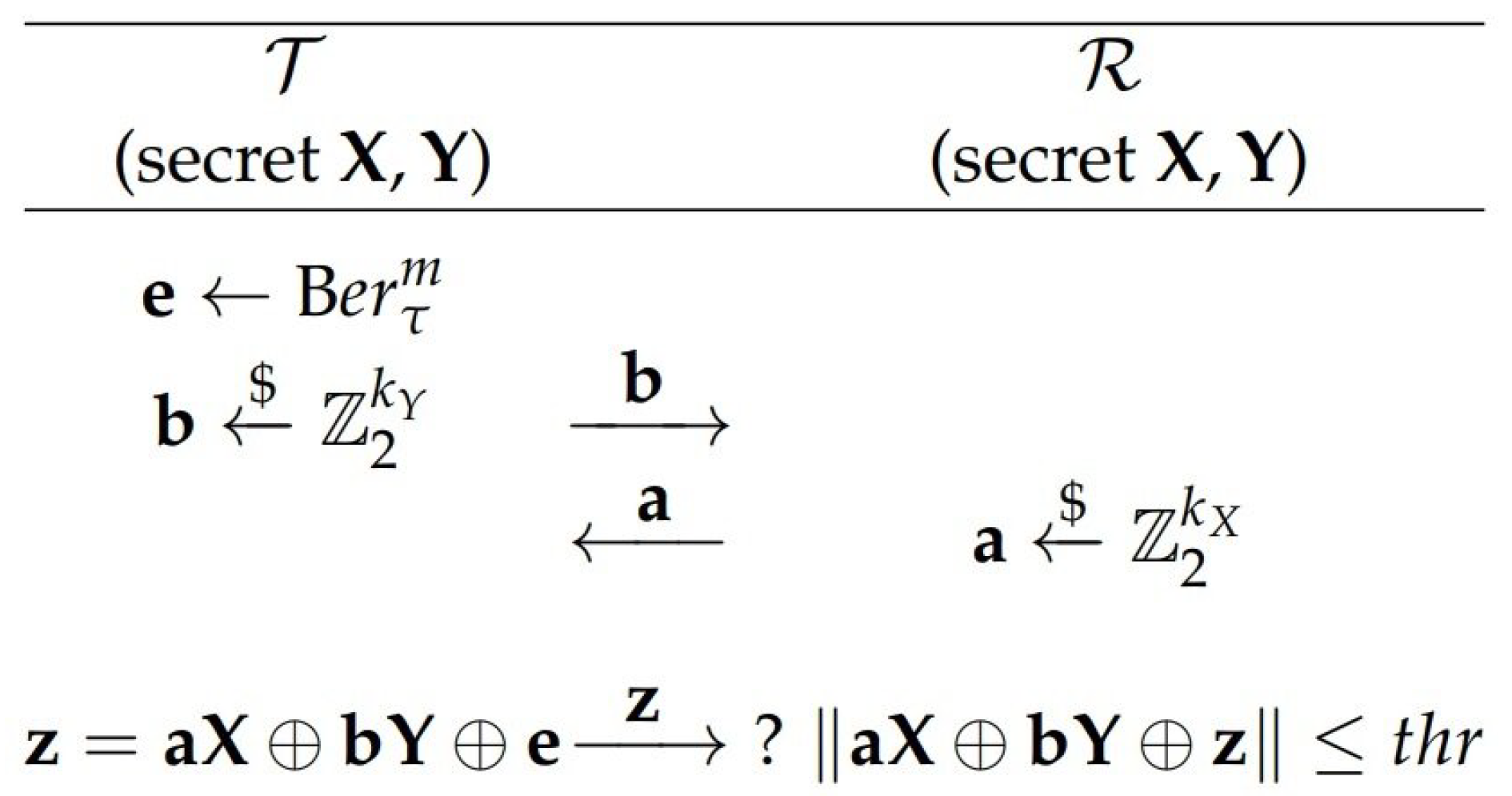
The HB family of authentication protocols has attracted a lot of attention because of their simple implementations and the provable security based on the well-known hard problem—Learning Parity with Noise (LPN). Random-HB# and HB# are prominent representatives of this family. Their authentication procedure consists of the following steps [11]—first, the Tag sends a random blinding vector to the Reader to initiate the authentication and the Reader responds with a random challenge vector to the Tag. Then Tag sends to the Reader, where is a noise vector whose bits independently follow Bernoulli distribution with coefficient , and are their shared secret keys (random matrices for Random-HB# and so-called Toeplitz matrices for HB#). The Reader validates the Tag, that is, accepts its response, if and only if the Hamming weight falls under a certain threshold value (see Figure 1). Standard parameters’ values for these protocols are given in Table 1.
- Collects a triplet of messages exchanged between the Tag and the Reader by eavesdropping one of their communication sessions
- Replaces each triplet of messages between the Tag and the Reader during n following communication sessions with a triplet
- Counts the number c of “ACCEPT” decisions of the Reader at the end of those n sessions.
The acceptance rate , as it turns out, leaks the critical information which reveals the secret values. More precisely, the theoretical analysis from [12] shows that:
where is the standard normal cumulative distribution function. This formula allows the adversary to estimate the Hamming weight using solely the empirical value , for n large enough (Algorithm 1 from [12]).
After the adversary discovers the Hamming weight of the noise vector , he can reconstruct the vector by flipping its bits (more precisely, he flips which secretly contains ) and measures weight of after the flipping. If the weight has increased, the flipped bit was 0, otherwise, it was 1. This way, he reconstructs the noise vector and obtains the linear combination since (Algorithm 2 from [12]). The whole previous procedure is repeated also for other modification triplets obtained by eavesdropping, until the adversary collects enough of these linear combinations to form a full system of linear equations. The secret keys and are then recovered as the solution to this system.
As illustrated above, in each corrupted communication session, the Reader computes:
and the Tag successfully authenticates iff , whereas in a regular session, the Tag successfully authenticates iff . This way, by creating the cumulative noise , the adversary manipulates the verification criterion of the Reader and changes its theoretical acceptance rate from to .
Let us provide a simple and useful characterization of the OOV attack Algorithm 1 [12] output by introducing the notion of “decision zones.”
Definition 1.
(“OOV decision zones”). OOV -decision zone is an interval such that OOV Algorithm 1 estimates as iff .
After eavesdropping a triplet, the adversary considers all weights of the noise vector possible. He decides that is , since P is a monotone decreasing function (see Figure 3a).
After flipping a bit in the noise vector, whose weight is previously estimated as , the adversary considers only two weights possible: and , so there are two decision zones — and (see Figure 3b).
In [12], the complexity of the OOV attack is estimated as an overall number of modified authentication sessions, which is minimized if the expected noise vector weight coincides with the so-called optimal weight when it is polynomial (for weights not near enough the optimal one, it becomes exponential). To achieve this, different strategies are introduced in [12], such as flipping the adequate number of last bits when before weight measurement, or removing the already recovered 1-bits when .
Also, ref [12] provides an optimized version of the attack which uses flipping block-by-block in the noise vector recovery process instead of bit-by-bit. However, it is observed empirically in [25] that the actual benefit that this optimized version brings is somewhat overestimated. An explanation was offered that it uses insufficient sample sizes for decision making when measuring the weights, which are further away from the optimal one.
3. Revision of the OOV Attack
The previous work [25] has shown that the OOV attack predominantly incorrectly estimates weights of noise vectors. The probability of key recovery, that is, efficiency of the attack, is shown to be significantly lower compared to the values claimed in [12]. For the standard parameter set II, the probability of correct key recovery is shown to be 0.158 in the case of HB# and in the case of Random-HB#. The analysis presented in [25] reveals that, in order to achieve the precision of key recovery claimed in [12], it is necessary to increase the number of intercepted authentications by 18% in the case of HB# and by 55% in the case of Random-HB#. Since the number of intercepted authentication sessions is the unit of the attack complexity, the complexity increases accordingly. Furthermore, the analysis from [25] shows that the weight estimation error cannot be corrected by taking a larger “sample” n, i.e., larger number of intercepted authentication sessions. On the contrary, by increasing the sample, the quality of the weight estimate worsens. So, for example, experimental evaluation on the standard parameter set II shows that the percentage of correctly estimated weights is only 5%, even if a very large number of modifications is used (for more details, see Section 4.4 in [25]).
This has led us to conduct a thorough revision of cryptanalysis from [12], which we provide in this Section. We shall prove that the attack’s erroneous output is caused by inadequate, non-Bayesian inference over improper, approximate probability distributions of acceptance rates, which cannot be improved due to Central limit theorem application limitations for these protocols. We identify the exact distributions and the exact error of the approximations from [12]. Then we employ Bayesian reasoning over the exact distributions to construct proper decision zones, and show how OOV weight decision making proposed in [12] deviates significantly from the proper, Bayesian one.
3.1. Revision of the Theoretical Analysis behind the OOV Weight Estimate
Here, we revise the derivation of approximations of acceptance rates used in the OOV weight estimate process and report their significant imprecision. Specifically, this derivation is given in the “Correctness” paragraph, Section 2.1 in [12].
3.1.1. Incorrect Claim that Cumulative Noise Vector Follows Binomial Distribution
The mentioned paragraph begins with calculation of the probability that i-th bit of cumulative noise vector is 1:
Then it says (exact quotation): “Hence, bits of follow a Bernoulli distribution of parameter and the other bits follow a Bernoulli distribution of parameter , thus follows a binomial distribution.” [12].
However, that is not correct: does not follow binomial distribution, because that is by definition a distribution of sum of independent and identically distributed Bernoulli trials i.e., of the same parameter (probability of success). Here, the Hamming weight of cumulative noise , as we can see, is a sum of Bernoulli trials of mixed parameter values or and actually corresponds to a more general so-called Poisson-Binomial Distribution. We elaborate more on this distribution in the upcoming Section 3.2.
3.1.2. Approximation of Acceptance Rates without Error Estimation
The “Correctness” paragraph [12] continues with the calculations of the expected weight of the vector as and its variance , which are correct, and derives approximation of acceptance rate during the attack:
where is the standard normal cumulative distribution function, by referring to the Central Limit Theorem (CLT)—Formula (1) in [12].
Here, ref [12] applies CLT to sum without discussing the magnitude of error of this approximation—the theorem itself only points to its convergence when .
3.1.3. Unknown Error Bound of the Weight Estimate Process
In the rest of the “Correctness” paragraph [12], the authors merge previous approximation (1) with the second one (which is a consequence of the Law of large numbers):
to conclude that:
The idea behind the merging of the two approximations can be explained in the following way: converges to when (by the Law of large numbers), while converges to 0 when (by the Central Limit Theorem). Thus, gets arbitrarily close to , if both n and m are large enough. This can be represented as:
Unlike , ref [12] actually does derive error for approximation, and how large n should be in order to make the error negligible:
with probability for (Formula (2) in [12]) where gets exponentially small as (i.e., n) increases asymptotically. Therefore, is used to estimate for n large enough.
However, as the final approximation (3) contains estimate whose error was not assessed in [12], its error is also unknown. The bound of the error for (3) is essential, because if these approximate values deviate too much from the actual values, it could lead to the wrong decision of . Let us remember that in the OOV attack the weight of noise vector is , if is closest to , for all possible values of .
3.1.4. Main Conclusions
We summarize the mistakes in the theoretical analysis behind the OOV attack from [12], found in the analysis given above, which will turn out as crucial for high error rate of the OOV weight estimate:
- The distribution of the Hamming weight of cumulative noise vector is wrongly assessed as Binomial,
- Approximation lacks error estimation,
- The error of the weight estimate procedure is unknown. Since error bound of is unknown, this consequently also stands for the final approximation which produces the output of weight estimate procedure.
In the following sections, we introduce our research process to overcome the listed omissions.
3.2. Error Estimation of Acceptance Rates Approximation
First, we infer the standard upper error bound of by applying Berry-Esseen inequality for CLT approximations. The obtained result indicates that distance between and could be too high and thus prevent a correct weight estimation. Then, we proceed to infer the exact distribution of the acceptance rates and the exact error of this approximation.
3.2.1. Standard Upper Error Bound for CLT Approximations
Approximation was derived in [12] using the CLT, which only implies its convergence when . The Berry-Eseen inequality further refines this result by providing bound on its maximal error. Here, we show that the sum follows Poisson-Binomial distribution, not the plain Binomial distribution as claimed in [12]. Then we apply a general CLT for non-identical random variables to this distribution in order to obtain , and we estimate its precision using the Berry-Eseen inequality.
Definition 2.
Poisson-Binomial distribution is a probability distribution of a sum of independent Bernoulli random variables with possibly different probabilities of success , and we denote it by . Binomial distribution is a special case of the Poisson-Binomial distribution where share the same probability of success.
Lemma 1.
The Hamming weight of cumulative noise vector , where , which the Reader computes in the verification phase after MIM modification of Random HB# or HB# protocol session, follows Poisson-Binomial distribution
.
Proof.
Since a new noise vector is being generated in each modification session, and remains fixed during all modifications, notice that:
where and are Bernoulli random variables, such that and (see Figure 4).
Therefore, . □
Theorem 1
(General CLT, Lyapunov condition [26]). Let be a sequence of independent (and not necessarily identical) random variables such that , and . If there is such that:
then the distributions of converge weakly to as , that is,
Theorem 2
(General CLT for Poisson-Binomial distribution). If random variable X follows Poisson-Binomial distribution i.e., , , where , and , then:
Proof of Theorem 2.
Let . We prove the Lyapunov condition is satisfied for .
Since , we have that:
Therefore and
□
Since and , as a direct consequence of Theorem 2 and Lemma 1, we have that:
Lemma 2.
For the cumulative noise vector it holds that:
In order to estimate the precision of this approximation, we proceed to use the standard error measure for general CLT:
Theorem 3
(Berry-Eseen inequality for non-identical random variables [27]). Let be independent random variables such that , , and . Then for every n there is an absolute constant C such that:
It was proven that ([28]). is the biggest known lower bound and the smallest known upper bound for C in literature, to the best of our knowledge.
Theorem 4
(Berry-Eseen inequality for Poisson-Binomial distribution). If random variable X follows Poisson-Binomial distribution, that is, , , where , and , then for every n there is a constant such that:
Proof.
Let , . Then and (see proof of Theorem 2). The claim follows directly by applying Berry-Eseen inequality to random variables . □
Lemma 3.
For the cumulative noise vector it holds that:
where .
Proof.
This is a direct consequence of the inequality above, taken in consideration that: , ,
,
,
. □
As a consequence of this Lemma, by taking , and , the standard Berry-Eseen upper bound estimate for the error of the approximation is:
where .
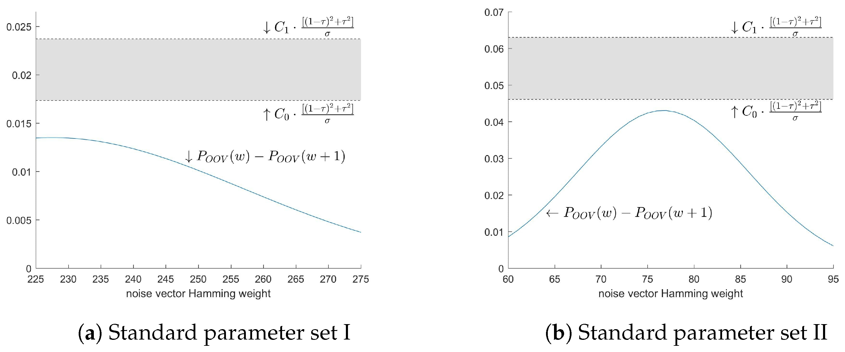
Using Formula (5) we derive that for the standard parameter set I, where and , the error upper bound lies in the interval , while for the standard parameter set II, where and , the error upper bound is from the interval .
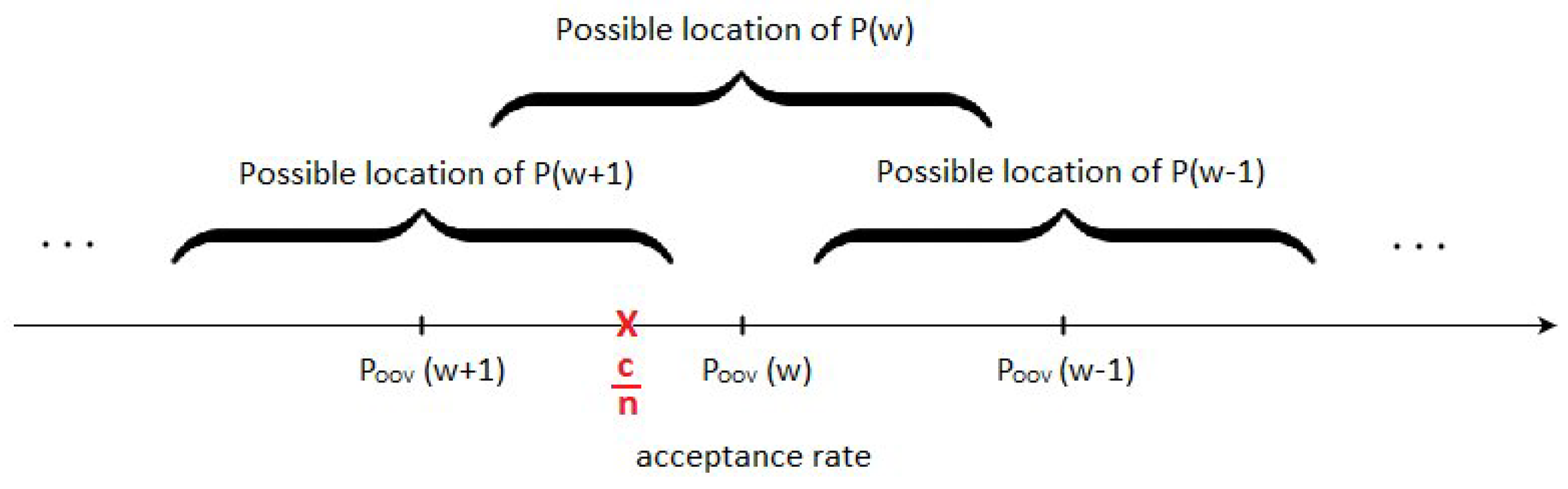
The exact lies somewhere in the interval . Nevertheless, this interval is wider, i.e., covers the interval in which the adversary has to decide between adjacent weights and (see Figure 5). It is possible that the adversary is incapable to determine and decide accurately if is closest to or , which directly jeopardizes his decision making. For example, if is in the position marked in Figure 6, the adversary will decide that the weight is , because is closest to it, but since is in a possible location of , it could in fact be closest to , and the actual weight could be . In order to investigate possibility of such scenarios of erroneous weight conclusions due to high error of approximation, in the next Section, we shall determine where precisely are values.
3.2.2. The Exact Distribution of the Acceptance Rates
Here, we calculate the exact acceptance rate of HB# and Random-HB# protocols while under the OOV attack, by using Lemma 1 from Section 3.2.1.
Theorem 5.
Let denote the probability of successful authentication after MIM modification using triplet of exchanged messages caught in a Random HB# or HB# protocol session, where . Then:
In addition, if c is the number of successful authentications after n MIM modifications, then for acceptance rate it holds that
Proof.
Since:
where , (see Proof of Lemma 1) we have that:
□
(Number of successes in Bernoulli experiments can not exceed . Similarly for .)
3.2.3. Exact Error of the Approximation
Finally, we are able to derive the exact error of the approximation as:
where and .
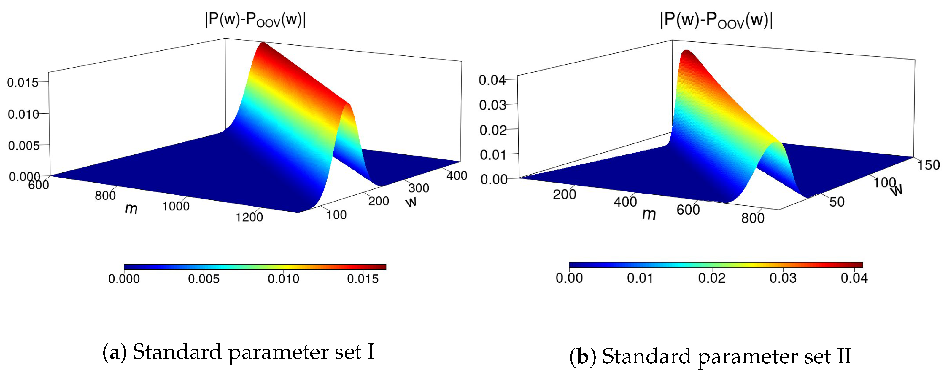
Although, in theory, this error diminishes for m large enough (see Figure 7), in the OOV attack m is the dimension of secret matrices. Thus, this error is a constant intrinsic to the protocol and the adversary is unable to manipulate it.
The exact error values for standard protocol parameters are shown in Figure 8.
Note that the error gets higher as approaches the claimed optimal weight , where it reaches its maximum. This weight is 228 for the standard parameter set I, while it is 77 for the other one.
3.3. Proper Decision Zones
The OOV decision zones, which are based on the inverse function values, have the following potential drawbacks, in general case:
- the inverse function might not preserve the ratios of distances, so, for example, it could be possible that is closer to than to , while is actually closer to than to ,
- is used as an approximation of exact acceptance rates P with unknown precision,
- should be determined by considering which of the possible distributions is most likely sampled from, i.e., by probabilistic reasoning, instead of simply applying the inverse function to value.
We employ the Bayesian reasoning over the exact distributions of acceptance rates to construct proper decision zones. The noise vector weight is estimated as if the observed empirical acceptance frequency most likely follows the exact distribution , where W is the set of all the weights the adversary considers possible.
As a general weight decision rule, , where is the probability of occurrence of noise vector whose weight is w. By its logarithmic transformation, we obtain that the adversary decides the noise vector weight as iff:
where , . After the mere eavesdropping, . If the eavesdropped vector was flipped in f positions to reach optimal weight, . When recovering bits, and . The values and may be calculated in advance, so decision making is highly efficient.
However, when considering weights near and standard parameter sets, for n large enough, the decision making can be further simplified. Namely, after comparing variances of the exact distributions for the consecutive weights , w and in such case, we have found their differences as insufficient to impact the Bayesian decision. Also, probabilities of occurrence of these weights produce negligible priors (observe division by n in ).
Therefore, because these distributions are almost symmetrical, for all practical purposes, -decision zones will be after eavesdropping, while they will be and when deciding between and after flipping a bit. We shall also call them “PB-decision zones", since they use the exact values . Figure 9 provides a graphical illustration of the PB-decision zones used in the processes of weight estimate after eavesdropping and bit recovery.
Expressed more formally—probability that is sampled from is , so according to maximum a posteriori (MAP) test, we choose hypothesis over iff that is,
that is, iff condition is satisfied, where , i.e., or when , or when , where . However, since for , and for , for weights near the optimal one, the condition is equivalent to . Furthermore, is negligible in such case, so we reduce this decision to condition , that is, that the observed frequency is closer to than to (P is monotone decreasing function).
3.4. The Exact and the Approximate Probability Distribution Relation
We now show that the decisions the adversary makes about noise vectors weights can differ depending on whether he uses the OOV approximation or the exact distribution.
We have noticed that the OOV w-decision zones are substantially shifted to the left with respect to PB-w decision zones, and that they often largely overlap with the correct PB- decision zone (see Figure 10). As a consequence, there is a high chance that the OOV adversary decides the weight is w, while the actual weight is .
This adverse phenomena is especially pronounced in the expected case—when is near the optimal weight , since there is the biggest distance between and —degrading significantly the precision of the weight estimate.
Furthermore, the shift of the OOV decision zones can not be repaired by employing larger “sample size” n, that is, number of intercepted authentications, because the approximation has a high fixed error in this scenario (as shown in the previous Section). The convergence occurs only when both and :
However, in the context of the OOV attack, m is a constant protocol parameter and thus:
This explains the experimental observations from [25] that the weight estimate does not improve by increasing the sample size.
4. Correction of the OOV Attack
In this section, we give a correction of the OOV-MIM attack and show that it meets the targeted precision, unlike the original attack.
4.1. Correction of the OOV Attack Algorithm
In order to solve the problem of high error of the approximation , we eliminate this approximation altogether, since we have shown that it can not be improved. Instead we employ the acceptance rates obtained from the exact distribution. That is, instead of:
we use Poisson-Binomial cumulative distribution function:
Then, we incorporate it in proper, Bayesian decision zones described in Section 3.3 with their corresponding optimal weights and modification samples. Noise vector Hamming weight will be estimated as if and only if is nearest to , for all weights considered possible.
Hence, the pseudocode of the proposed correction of the weight estimate procedure is given in Algorithm 1:
| Algorithm 1PB-OOV weight estimate alg. Approximating |
|
Since the PB Decision zone for , where we have that:
.
Therefore, after the eavesdropping, PB-OOV adversary chooses sample of size , to achieve the required precision , which is based on exact values instead of approximate ones as in Formula (2) from [12]. Accordingly, he uses optimal weight which minimizes this sample across all weights and its value is 229 for parameter set I, and 78 for parameter set II. After the flipping, he will use samples of size to recover bits.
It should be noted that the values can be calculated in advance, as a part of the preprocessing step, and stored in a table to be later used during the attack.
4.2. Comparison of the OOV and PB-OOV Attack Success
In this section we analyze the probability of success of the OOV and PB-OOV attack. Namely, we derive the probability the OOV adversary will correctly reconstruct a noise vector (and consequently recover the key) and show that, as a consequence of the approximation employed, the OOV attack is significantly less efficient than claimed in [12]. Oppositely, the PB-OOV attack proposed in Section 4.1, achieves the desired precision and efficiency.
4.2.1. Noise Vector Hamming Weight Estimate
OOV adversary. First, let us observe the distribution of acceptance rate during the attack when :
where .
The probability that the OOV adversary estimates that noise vector has weight , when its weight is (which may or may not be equal to ), using n modifications of authentication sessions is:
Therefore, the adversary makes correct decision when , using n modifications, with probability .
After evaluating Formula (8), we have found that the weight will either be estimated as one lower (when the adversary is wrong, which is the majority of the time for the weights near the expected ones) or make a correct guess, that is, all other cases will appear with negligible probability (see Table 2). This supports the experimental findings from [25]. Table 2 shows comparison between the claimed and real precision of the OOV weight estimate (see Appendix A Table A1 for details on the parameters’ values). It can be noticed that, for parameter set II, in the case of Random-HB#, the claimed precision is by two orders of magnitude smaller than the claimed. In all other cases, the discrepancy is somewhat smaller but, still, the real precision is by an order of magnitude smaller than the claimed.
PB-OOV adversary. Since is PB-w decision zone after the eavesdropping, and PB-OOV adversary uses exact values instead of the approximate ones , by analogous analysis as above, we obtain that he estimates the weight as when its actual value is with probability:
Unlike the OOV weight estimate, whose precision is shown to be remarkably lower than the claimed, precision of the PB-OOV weight estimate is within the given boundaries (see Table 3). This is also confirmed by the experimental results presented in Section 5.3.
4.2.2. Noise Vector Bits Recovery
Here, we compare the success rate of the OOV adversary and PB-OOV adversary when it comes to the reconstruction of noise vectors, that is, bit recovery.
OOV adversary. After the adversary has estimated the weight of the observed vector as after eavesdropping, he tries to recover its bits by flipping one by one each bit and estimating new weight as or . If the weight has decreased, he concludes the flipped bit is 1, otherwise, that the bit is 0. Therefore, he recovers a bit correctly, depending on its value, with probabilities:
The results of evaluation of Formula (9) are shown in Table 4. First, it should be noted that the probability for bit recovery is very asymmetrical, that is, the precision for 0-bit recovery is very different from the precision for 1-bit, while the claimed precision is uniform for both bit values. Secondly, when the weight is correctly estimated, the precision for 0-bit is much lower than the claimed and it would make reconstruction of the noise vector (and further the key recovery itself) practically impossible. This is in accordance with the experimental results from [25]. On the other hand, the OOV adversary has more success in bits recovery when the initial weight estimate is incorrect, since the relative change remains intact if the measured weights are both one lower than the actual ones. The two errors made in the weight estimate processes can neutralize each other; however, even with this mutual cancellation of the errors, the claimed precision is not achieved. Namely, the precision for 1-bit recovery is lower than the targeted and that lowers the probability of the attack success.
Let us further consider the probability that the OOV adversary will successfully recover a complete noise vector. We observe the expected case ( for parameter set II). As we have already noted: (a) is either or , and (b) the noise vector is practically impossible to recover when due to too high error for 0-bit. Thus, for parameter set II, the probability of the OOV Adversary successfully recovering a complete m-bit noise vector of weight is:
where .
Similarly, for parameter set I, the adversary needs to recover and remove errors in a noise vector in order to achieve the optimal weight. This is expected to happen after recovering bits, thus:
where: .
Using Formulas (10) and (11) we can evaluate the probability that the OOV adversary will correctly recover a complete noise vector in the expected case, and compare the obtained probability with the claimed one, which is calculated based on the claimed probabilities of correct weight estimate and bit guess as . Results of the comparison are given in Table 5. Although the difference between the claimed and real precision on the noise vector level does not seem remarkable for Random-HB#, it does make a significant impact on the key recovery probability, having in mind the number of noise vector that have to be reconstructed, which is 592. More details will be provided in the next Section 4.2.3.
PB-OOV adversary. For the PB-OOV adversary, by replacing with P, and with (i.e., by using proper PB -decision zones) in the derivation above, the probabilities of successful bit recovery, depending on its value are:
Table 6 shows the precision the PB-OOV adversary achieves in the bit recovery process, when the standard parameter sets are employed. The results obtained by evaluating Formula (12) prove that the PB-OOV on the bit level does achieve the targeted precision using the OOV sample (i.e., the number of modifications). This is also confirmed by the experimental results presented in Section 5.3.
Further, we analyze the probability that the PB-OOV adversary will successfully recover a complete noise vector. We observe the expected case ( for parameter set II). For parameter set II, the probability is given by the formula:
where .
Similarly, for parameter set I, we have that:
where , , , , , .
4.2.3. Secret Keys Recovery Comparison
Finally, let us compare the precision of the OOV attack and PB-OOV attack. We observe the expected case ( for parameter set II). Let l be the number of secret bits, that is, secret key length and m be the noise vector length. The claimed probability of key recovery in [12] is calculated as . This probability is equal .
As we have shown in Section 4.2.2, the PB-OOV attack achieves the claimed precision on bit level, therefore it can recover the secret key with probability 0.37. Let us further compare this value with the probability that the OOV adversary recovers the key. In the case of Random-HB#, the number of secret bits is and the adversary has to recover complete noise vectors of length m. The probability of a key recovery can be calculated using the values from Table 5 as . For parameter set I, the probability of key recovery is , and for parameter set II, it is equal . This is remarkably smaller than the claimed 0.37. In the case of HB#, the adversary has to recover complete noise vectors and additional bits. For parameter set I, the probability of key recovery for HB# is 0.024, and for parameter set II, it is 0.159.
More formally, the OOV attack reconstructs the secret keys if it recovers:
- -
- whole m-bit noise vectors—which happens with probability ,
- -
- and then the remaining bits, by guessing incorrectly one more noise vector weight, and recovering each one of them—which happens with probability for parameter set II andfor parameter set I, since .
Therefore, the probability of successful recovery of secret keys using OOV attack will be:
and similarly, probability of successful recovery of secret keys using PB-OOV attack is:
where is the same as , but with symbols instead of p.
Complexity comparison. The complexity of the OOV attack needed to achieve the required (claimed) key recovery rate is . By increasing the number of modifications n until the claimed key recovery rate is reached, we have estimated that the complexity of the OOV attack is higher than the claimed—for parameter set II by 55% in the case of Random-HB# and by 18% for HB# (this supports the results from [25] based on experimental evaluation), and for parameter set I by 150% in the case of Random-HB# and 35% for HB#. On the other hand, since the PB-OOV attack achieves the required precision on a bit recovery level targeted in [12], its precision and complexity is in accordance with the one claimed for the original OOV attack.
5. Experimental Results and Discussion
5.1. Evaluation of the Acceptance Rates
We have conducted a set of experiments to confirm the convergence of experimentally obtained acceptance rates to the corresponding PB values. There were 4 rounds of tests, for , , n = 10,000 and n = 15,000. For each n, we generated 500 noise vectors and flipped the appropriate number of their last bits, so that the expected weight of the noise vectors is optimal, that is, 78. For each test vector , we measured the acceptance rate and analyzed how it relates to and . In general, it can be noted that the experimental acceptance rates lie above the corresponding OOV points, but compared to the corresponding PB points, they are evenly distributed above and bellow (see Figure 11). It can also be noticed that as n increases, the experimental points concentrate around the PB points, as expected. This further explains and confirms that the OOV algorithm relaying on the OOV approximation has high error rate when it comes to weight estimate, while the corrected PB-OOV algorithm gives much better results.
Furthermore, we compare experimentally obtained acceptance rates with OOV and PB reference points, i.e., and , using a standard error measure—Mean absolute error (MAE), and show how it relates to the correctness of weight estimates. That is, for a set of test noise vectors, we observe the MAE between the acceptance rates , where n is the number of intercepted authentication sessions (i.e., modifications), and and :
Consequently, the expected MAE value for the OOV points, across all possible weights , as , converges to:
since , after flipping f last bits in , while for the PB points they converge to:
This is in accordance with the experimental results shown in Figure 12, for different number of modifications n. Furthermore, Figure 12 and Figure 13 show that there is an inverse correlation between the distance (between the experimental and OOV points, i.e., PB points, respectively) and the accuracy of weight estimation.
5.2. Precision Comparison of the OOV and PB-OOV Weight Estimate: Experimental
Here, the differences in the weight estimate quality between the original OOV Algorithm 1 and the PB-OOV Algorithm 1 proposed in Section 4.1 are experimentally proven. We have analyzed and compared effectiveness of the two algorithms for different Hamming weights. For the standard parameter set I, 99% of all noise vectors have the weight between 250 and 330. The comparison of the algorithms is based on the sample of 5000 noise vectors whose Hamming weight is from that interval. The number of modifications employed for weight estimation corresponds to the HB# scenario. The success rate of the OOV algorithm is 20% and for the PB-OOV it is 98%. Detailed results are given in Figure 14a. For the standard parameter set II, 99% of all noise vectors have the weight between 60 and 95 (this is after flipping bits to obtain a vector of the optimal weight from a vector of the expected weight) and the comparison of the two algorithms is based on the sample of 5000 noise vectors with the Hamming weight in this interval. The number of modifications employed for weight estimation corresponds to the HB# scenario. The experimental results again show that the success rate of the OOV algorithm is much worse than PB-OOV (11% in contrast to 99%). Details are given in Figure 14b.
5.3. Evaluation of the PB-OOV Attack Precision
In Section 2.1 from [12], the authors derive the error formula and calculate the number of modifications n that should provide the aimed accuracy of the OOV attack, that is, of the weight estimate and bit recovery. However, the analysis given in Section 4.2 shows that the precision deviates significantly from the one claimed. The analysis provides the theoretical proof that supports the experimental findings presented in [25]. On the other hand, the analysis of the proposed PB-OOV algorithm given in Section 4.2, shows that this algorithm does achieve the desired precision and efficiency. We have conducted a series of experiments in order to experimentally verify the correctness of the PB-OOV attack. The experimental results presented in this section support the conclusions of the theoretical analysis.
The tests are conducted for both HB# and Random-HB# protocols and parameter set II. The number of modifications used (“sample size”) is the one from the [12]. For the HB# protocol we have tested the weight estimate and bit recovery precision for 2000 randomly generated noise vectors of the optimal weight. The weights of two noise vector were incorrectly estimated as 79, since the obtained acceptance rates were 0.473227 and 0.475217. This gives success rate of 0.999 in weight estimation step. When the weight of a vector is incorrectly guessed, it further causes high error rate in the bit recovery process, since the algorithm relies on the initial weight estimate and chooses between and after flipping the observed bit. However, when the weight estimate is correct, targeted bit precision is , and our tests verify that the PB-OOV attack complies with this. Namely, in the set of noise vectors whose weight is correctly estimated, the average bit guessing success rate in our test is 0.999342, compared to the targeted 0.999320. For Random-HB#, we have randomly generated 25,000 noise vectors of the optimal weight. The PB-OOV attack correctly estimated all weights, while the achieved average bit guessing success rate was 0.999996, which is in line with the targeted precision. An interesting finding regarding the OOV attack is that the bit guessing precision may significantly differ for 0-bits and 1-bits, for example, in the case of HB# and parameter set II, precision for 0-bit is 0.764623, while for 1-bit it is remarkably higher and equal (see Table 4). On the other hand, the proposed PB-OOV algorithm does not have this strong and distinct bias. Table 8 summarizes the results of the tests.
6. Conclusions
This paper provides a detailed examination of the OOV attack reported in [12] against the LPN based authentication protocols known as HB# and Random-HB#. We have found that the problem of discrepancy between the theoretically estimated performances and complexity in [12] and the experimentally evaluated ones in [25] arises from non-Bayesian reasoning with inadequate approximations of the probability distributions on the acceptance rates during the attack, which can not be improved due to the limitations of Central limit theorem use in the attack context. We give a correction of the attack by employing proper, Bayesian inference after establishing the exact underlying probability distributions, and prove that the new version of the attack, unlike the original one, achieves the targeted precision and complexity.
Since the OOV attack is recognized as one of the cornerstones in the analysis of any HB-like authentication protocol, our correction of the OOV attack is not only significant against Random-HB# and HB#, but also for practical security analysis of all new members of the HB-family. An interesting future direction could be a design of improved MIM attacks against HB-like protocols, which could be based on the corrected version of the OOV attack proposed in this paper.
Author Contributions
Conceptualization, S.T., M.K. and M.J.M.; formal analysis, S.T. and M.K.; funding acquisition, S.T., M.K. and M.J.M.; investigation, S.T., M.K.; methodology, S.T., M.K., and M.J.M.; software, M.K., S.T.; validation, S.T. and M.K.; writing—original draft, S.T., M.K. and M.J.M. All authors have read and agreed to the published version of the manuscript.
Funding
This research has been supported by the Ministry of education, science and technological development, Government of Serbia.
Institutional Review Board Statement
Not applicable.
Informed Consent Statement
Not applicable.
Data Availability Statement
Not applicable.
Conflicts of Interest
The authors declare no conflict of interest.
Appendix A

Table A1.
Parameters’ values used in the OOV and PB-OOV attack.
| Parameter Set I | Parameter Set II | |||
|---|---|---|---|---|
| HB# | Random-HB# | HB# | Random-HB# | |
| 2.401 | 3.308 | 2.265 | 3.164 | |
| 16,780.41 * | 269.39 | |||
| 2742.61 | ||||
| 15,789.60 | 270.95 | |||
| 2743.75 | ||||
| 96,736 | 183,626 | 1382 | 2697 | |
| 15,811 | 30,012 | |||
| 91,024 | 172,783 | 1390 | 2712 | |
| 15,817 | 30,024 | |||
* Rexp is calculated using Formula (2) from the OOV paper [12].
References
- Avoine, G.; Carpent, X.; Hernandez-Castro, J. Pitfalls in ultralightweight authentication protocol designs. IEEE Trans. Mob. Comput. 2015, 15, 2317–2332. [Google Scholar] [CrossRef]
- Baashirah, R.; Abuzneid, A. Survey on prominent RFID authentication protocols for passive tags. Sensors 2018, 18, 3584. [Google Scholar] [CrossRef] [PubMed] [Green Version]
- D’Arco, P. Ultralightweight cryptography. In International Conference on Security for Information Technology and Communications; Springer: Cham, Switzerland, 2018; pp. 1–16. [Google Scholar]
- Hopper, N.J.; Blum, M. Secure Human Identification Protocols. In Advances in Cryptology—ASIACRYPT 2001. ASIACRYPT 2001. Lecture Notes in Computer Science; Boyd, C., Ed.; Springer: Berlin/Heidelberg, Germany, 2001; Volume 2248. [Google Scholar]
- Katz, J.; Shin, J.S. Parallel and Concurrent Security of the HB and HB+ Protocols. In Advances in Cryptology—EUROCRYPT 2006. EUROCRYPT 2006. Lecture Notes in Computer Science; Vaudenay, S., Ed.; Springer: Berlin/Heidelberg, Germany, 2006; Volume 4004. [Google Scholar]
- Katz, J.; Shin, J.S.; Smith, A. Parallel and concurrent security of the HB and HB+ protocols. J. Cryptol. 2010, 23, 402–421. [Google Scholar] [CrossRef] [Green Version]
- Gilbert, H.; Robshaw, M.; Sibert, H. Active attack against HB+: A provably secure lightweight authentication protocol. Electron. Lett. 2005, 41, 1169–1170. [Google Scholar] [CrossRef] [Green Version]
- Bringer, J.; Chabanne, H.; Dottax, E. HB++: A Lightweight Authentication Protocol Secure against Some Attacks. In Proceedings of the Second International Workshop on Security, Privacy and Trust in Pervasive and Ubiquitous Computing (SecPerU’06), Lyon, France, 29 June 2006; IEEE Computer Society: Washington, DC, USA, 2006; pp. 28–33. [Google Scholar]
- Munilla, J.; Peinado, A. HB-MP: A further step in the HB-family of lightweight authentication protocols. Comput. Netw. 2007, 51, 2262–2267. [Google Scholar] [CrossRef]
- Gilbert, H.; Robshaw, M.J.; Seurin, Y. Good variants of HB+ are hard to find. In Financial Cryptography and Data Security; Springer: Berlin/Heidelberg, Germany, 2008; pp. 156–170. [Google Scholar]
- Gilbert, H.; Robshaw, M.J.B.; Seurin, Y. HB#: Increasing the Security and Efficiency of HB+. In Advances in Cryptology—EUROCRYPT 2008. Lecture Notes in Computer Science; Smart, N., Ed.; Springer: Berlin/Heidelberg, Germany, 2008; Volume 4965. [Google Scholar]
- Ouafi, K.; Overbeck, R.; Vaudenay, S. On the Security of HB# against a Man-in-the-Middle Attack. In Advances in Cryptology—ASIACRYPT 2008. Lecture Notes in Computer Science; Pieprzyk, J., Ed.; Springer: Berlin/Heidelberg, Germany, 2008; Volume 5350. [Google Scholar]
- Leng, X.; Mayes, K.; Markantonakis, K. HB-MP+ protocol: An improvement on the HB-MP protocol. In Proceedings of the 2008 IEEE International Conference on RFID, Las Vegas, NV, USA, 16–17 April 2008; IEEE: Piscataway, NJ, USA, 2008; pp. 118–124. [Google Scholar]
- Yoon, B.; Sung, M.Y.; Yeon, S.; Oh, H.S.; Kwon, Y.; Kim, C.; Kim, K.H. HB-MP++ protocol: An ultra lightweight authentication protocol for RFID system. In Proceedings of the 2009 IEEE International Conference on RFID, Orlando, FL, USA, 27–28 April 2009; IEEE Computer Society: Washington, DC, USA, 2009; pp. 186–191. [Google Scholar]
- Aseeri, A.; Bamasak, O. HB-MP*: Towards a Man-in-the-Middle-Resistant Protocol of HB Family. In 2nd Mosharaka International Conference on Mobile Computing and Wireless Communications (MIC-MCWC 2011); Mosharaka for Research and Studies: Amman, Jordan, 2011; Volume 2, pp. 49–53. [Google Scholar]
- Bringer, J.; Chabanne, H. Trusted-HB: A low-cost version of HB+ secure against man-in-the-middle attacks. IEEE Trans. Inf. Theory 2008, 54, 4339–4342. [Google Scholar] [CrossRef]
- Madhavan, M.; Thangaraj, A.; Sankarasubramanian, Y.; Viswanathan, K. NLHB: A non-linear HopperBlum protocol. In Proceedings of the 2010 IEEE International Symposium on Information Theory, Austin, TX, USA, 13–18 June 2010; IEEE: Piscataway, NJ, USA, 2010; pp. 2498–2502. [Google Scholar]
- Bosley, C.; Haralambiev, K.; Nicolosi, A. HBN: An HB-like protocol secure against man-in-the-middle attacks. IACR Cryptol. ePrint Arch. 2011, 2011, 350. [Google Scholar]
- Rizomiliotis, P.; Gritzalis, S. GHB#: A provably secure HB-like lightweight authentication protocol. In International Conference on Applied Cryptography and Network Security; Springer: Berlin/Heidelberg, Germany, 2012; pp. 489–506. [Google Scholar]
- Hammouri, G.; Öztürk, E.; Birand, B.; Sunar, B. Unclonable lightweight authentication scheme. In International Conference on Information and Communications Security; Springer: Berlin/Heidelberg, Germany, 2008; pp. 33–48. [Google Scholar]
- Hammouri, G.; Sunar, B. PUF-HB: A tamper-resilient HB based authentication protocol. In International Conference on Applied Cryptography and Network Security; Springer: Berlin/Heidelberg, Germany, 2008; pp. 346–365. [Google Scholar]
- Deng, G.; Li, H.; Zhang, Y.; Wang, J. Tree-LSHB+: An LPN-based lightweight mutual authentication RFID protocol. Wirel. Pers. Commun. 2013, 72, 159–174. [Google Scholar] [CrossRef]
- Qian, X.; Liu, X.; Yang, S.; Zuo, C. Security and privacy analysis of tree-LSHB+ protocol. Wirel. Pers. Commun. 2014, 77, 3125–3314. [Google Scholar] [CrossRef]
- Karrothu, A.; Scholar, R.; Norman, J. An analysis of LPN based HB protocols. In Proceedings of the 2016 Eighth International Conference on Advanced Computing (ICoAC), Chennai, India, 19–21 January 2017; IEEE: Piscataway, NJ, USA, 2017; pp. 138–145. [Google Scholar]
- Knežević, M.; Tomović, S.; Mihaljević, M.J. Man-In-The-Middle Attack against Certain Authentication Protocols Revisited: Insights into the Approach and Performances Re-Evaluation. Electronics 2020, 9, 1296. [Google Scholar] [CrossRef]
- Koralov, L.; Sinai, Y.G. Theory of Probability and Random Processes; Springer: Berlin/Heidelberg, Germany, 2007; pp. 131–134. [Google Scholar]
- Shiganov, I.S. Refinement of the upper bound of the constant in the central limit theorem. J. Math. Sci. 1986, 35, 2545–2550, (translated from Stab. Probl. Stoch. Models 1982, 105–115.). [Google Scholar] [CrossRef]
- Shevtsova, I.G. An improvement of convergence rate estimates in the Lyapunov theorem. Dokl. Math. 2010, 82, 862–864. [Google Scholar] [CrossRef]
Figure 1.
Random-HB# and HB# authentication protocols.

Figure 2.
The OOV attack against Random-HB# and HB#.

Figure 3.
Decision making of the OOV attack Algorithm 1.

Figure 4.
Distribution structure of the cumulative noise vector .

Figure 5.
The approximation error upper bound is larger than the interval widths used in the attack. Thus, the adversary may not be capable to accurately estimate noise vectors weights.
Figure 5.
The approximation error upper bound is larger than the interval widths used in the attack. Thus, the adversary may not be capable to accurately estimate noise vectors weights.

Figure 6.
Localization of values using Berry-Eseen upper error bound.

Figure 7.
Theoretically, the approximation error decreases as m increases by CLT (note the transition in color of the error peak). In the OOV attack, or , for standard parameter sets I or II, respectively.
Figure 7.
Theoretically, the approximation error decreases as m increases by CLT (note the transition in color of the error peak). In the OOV attack, or , for standard parameter sets I or II, respectively.

Figure 8.
The exact error of the approximation.

Figure 9.
PB-decision zones used after eavesdropping (left) and for bit recovery (right).

Figure 10.
Different “decision zones” according to the OOV approximation and the exact Poisson-Binomial distribution.
Figure 10.
Different “decision zones” according to the OOV approximation and the exact Poisson-Binomial distribution.

Figure 11.
Comparison of the experimentally obtained acceptance rates and the corresponding and points for n = 2500, 5000, 10,000, 15,000.
Figure 11.
Comparison of the experimentally obtained acceptance rates and the corresponding and points for n = 2500, 5000, 10,000, 15,000.

Figure 12.
MAE between the experimentally obtained acceptance rates and the OOV and PB points, respectively, for n = 2500, 5000, 10,000 and 15,000.
Figure 12.
MAE between the experimentally obtained acceptance rates and the OOV and PB points, respectively, for n = 2500, 5000, 10,000 and 15,000.

Figure 13.
Percentage of correct weights estimates based on acceptance rates using the PB distribution and OOV approximation respectively, for n = 2500, 5000, 10,000 and 15,000.
Figure 13.
Percentage of correct weights estimates based on acceptance rates using the PB distribution and OOV approximation respectively, for n = 2500, 5000, 10,000 and 15,000.

Figure 14.
Precision comparison of the weight estimate using the OOV and PB-OOV algorithms.

Table 1.
Standard parameter sets I and II for HB# and Random-HB# proposed in [11]. Number l of secret bits is for Random-HB#, while it is for HB#.
Table 1.
Standard parameter sets I and II for HB# and Random-HB# proposed in [11]. Number l of secret bits is for Random-HB#, while it is for HB#.
| Parameter Set | m | ||||
|---|---|---|---|---|---|
| I | 80 | 512 | 1164 | 0.25 | 405 |
| II | 80 | 512 | 441 | 0.125 | 113 |
Table 2.
Comparison of the claimed and real precision of the OOV weight estimate showing that the real precision is remarkably smaller than the claimed one.
Table 2.
Comparison of the claimed and real precision of the OOV weight estimate showing that the real precision is remarkably smaller than the claimed one.
| Parameter Set I | Parameter Set II | |||
|---|---|---|---|---|
| HB# | Random-HB# | HB# | Random-HB# | |
| claimed precision | 0.999315 | 0.999997 | 0.998641 | 0.999992 |
| real precision | 0.087803 | 0.031017 | 0.038852 | 0.006860 |
| 0.912197 | 0.968983 | 0.961146 | 0.993139 | |
Table 3.
Precision of the proposed PB-OOV algorithm meets the targeted precision for weight estimate.
Table 3.
Precision of the proposed PB-OOV algorithm meets the targeted precision for weight estimate.
| Parameter Set I | Parameter Set II | |||
|---|---|---|---|---|
| HB# | Random-HB# | HB# | Random-HB# | |
| targeted precision | 0.999315 | 0.999997 | 0.998641 | 0.999992 |
| real precision | 0.999506 | 0.999998 | 0.998641 | 0.999992 |
Table 4.
Comparison of the claimed and real precision of the OOV bit recovery depending on the initial weight estimate.
Table 4.
Comparison of the claimed and real precision of the OOV bit recovery depending on the initial weight estimate.
| Parameter Set I | Parameter Set II | |||
|---|---|---|---|---|
| HB# | Random-HB# | HB# | Random-HB# | |
| claimed precision | 0.999658 | 0.9999986 | 0.999320 | 0.999996 |
| 0.858089 | 0.930114 | 0.764623 | 0.843169 | |
| 0.365592 | 0.317990 | |||
| 0.991712 | 0.999518 | 0.993508 | 0.999740 | |
| 0.999908 | ||||
| 0.999997 | 0.999957 | |||
| 0.998863 | 0.999987 | |||
Table 5.
Comparison of the claimed and real precision of the OOV noise vector recovery showing that the real precision is smaller than the claimed one.
Table 5.
Comparison of the claimed and real precision of the OOV noise vector recovery showing that the real precision is smaller than the claimed one.
| Parameter Set I | Parameter Set II | |||
|---|---|---|---|---|
| HB# | Random-HB# | HB# | Random-HB# | |
| claimed precision | 0.670720 | 0.998314 | 0.739967 | 0.998306 |
| 0.245168 | 0.932141 | 0.573019 | 0.973427 | |
Table 6.
Precision of the proposed PB-OOV algorithm meets the targeted precision for bit recovery.
| Parameter Set I | Parameter Set II | |||
|---|---|---|---|---|
| HB# | Random-HB# | HB# | Random-HB# | |
| targeted precision | 0.999658 | 0.9999986 | 0.999320 | 0.999996 |
| 0.999623 | 0.9999983 | 0.999345 | 0.999996 | |
| 0.999660 | 0.9999986 | |||
| 0.999874 | 0.9999998 | 0.999351 | 0.999996 | |
| 0.999659 | 0.9999986 | |||
Table 7.
Precision of the proposed PB-OOV algorithm meets the targeted precision for noise vector recovery.
Table 7.
Precision of the proposed PB-OOV algorithm meets the targeted precision for noise vector recovery.
| Parameter Set I | Parameter Set II | |||
|---|---|---|---|---|
| HB# | Random-HB# | HB# | Random-HB# | |
| claimed precision | 0.670720 | 0.998314 | 0.739967 | 0.998306 |
| 0.698279 | 0.998538 | 0.749770 | 0.998443 | |
Table 8.
PB-OOV experimentally obtained precision.
| HB# | Random-HB# | |
|---|---|---|
| num. tests | 2000 | 25,000 |
| targeted OOV weight est. precision | 0.998641 | 0.999992 |
| experimentally obtained weight est. precision | 0.999 | 1 |
| targeted OOV bit precision | 0.999320 | 0.999996 |
| experimentally obtained avg. bit precision | 0.999342 | 0.999996 |
| experimentally obtained 0-bit precision | 0.999344 | 0.999996 |
| experimentally obtained 1-bit precision | 0.999333 | 0.999995 |
Publisher’s Note: MDPI stays neutral with regard to jurisdictional claims in published maps and institutional affiliations. |
© 2021 by the authors. Licensee MDPI, Basel, Switzerland. This article is an open access article distributed under the terms and conditions of the Creative Commons Attribution (CC BY) license (http://creativecommons.org/licenses/by/4.0/).
Share and Cite
MDPI and ACS Style
Tomović, S.; Knežević, M.; Mihaljević, M.J. Analysis and Correction of the Attack against the LPN-Problem Based Authentication Protocols. Mathematics 2021, 9, 573. https://doi.org/10.3390/math9050573
AMA Style
Tomović S, Knežević M, Mihaljević MJ. Analysis and Correction of the Attack against the LPN-Problem Based Authentication Protocols. Mathematics. 2021; 9(5):573. https://doi.org/10.3390/math9050573
Chicago/Turabian StyleTomović, Siniša, Milica Knežević, and Miodrag J. Mihaljević. 2021. "Analysis and Correction of the Attack against the LPN-Problem Based Authentication Protocols" Mathematics 9, no. 5: 573. https://doi.org/10.3390/math9050573
Note that from the first issue of 2016, this journal uses article numbers instead of page numbers. See further details here.