A Generalized Viscosity Inertial Projection and Contraction Method for Pseudomonotone Variational Inequality and Fixed Point Problems

Abstract

We introduce a new projection and contraction method with inertial and self-adaptive techniques for solving variational inequalities and split common fixed point problems in real Hilbert spaces. The stepsize of the algorithm is selected via a self-adaptive method and does not require prior estimate of norm of the bounded linear operator. More so, the cost operator of the variational inequalities does not necessarily needs to satisfies Lipschitz condition. We prove a strong convergence result under some mild conditions and provide an application of our result to split common null point problems. Some numerical experiments are reported to illustrate the performance of the algorithm and compare with some existing methods.

1. Introduction

Let H be a real Hilbert space induced with norm $\parallel ·\parallel$ and inner product $\langle ·,·\rangle .$ Let $\mathsf{\Omega }$ be a nonempty, closed and convex subset of H and $A:\mathsf{\Omega }\to H$ be an operator. We study the Variational Inequality Problem (shortly, VIP) defined by

$$\mathrm{find}{x}^{*}\in \mathsf{\Omega }\mathrm{such}\mathrm{that}\langle A{x}^{*},u-x^{*}\rangle \ge 0\forall u\in \mathsf{\Omega }.$$

(1)

The solution set of (1) is denoted by $\mathcal{S}.$ The VIP is a powerful tool for studying many nonlinear problems arising in mechanics, optimization, control network, equilibrium problems, and so forth; see References [1,2,3]. Due to this importance, the problem has drawn the attention of many researchers who had studied its existence of solution and proposed various iterative methods such as the extragradient method [4,5,6,7,8,9], subgradient extragradient method [10,11,12,13,14], projection and contraction method [15,16], Tseng’s extragradient method [17,18] and Bregman projection method [19,20] for approximating its solution in various dimensions.

The operator $A:\mathsf{\Omega }\to H$ is said to be

• $\beta$-strongly monotone on $\mathsf{\Omega }$ if there exists $\beta >0$ such that

  $$\langle Ax-Ay,x-y\rangle \ge \beta \parallel x-y\parallel \forall x,y\in \mathsf{\Omega };$$
• monotone on $\mathsf{\Omega }$ if

  $$\langle Ax-Ay,x-y\rangle \ge 0\forall x,y\in \mathsf{\Omega };$$
• $\gamma$- strongly pseudo-monotone on $\mathsf{\Omega }$ if there exists $\eta >0$ such that

  $$\langle Ax,y-x\rangle \ge 0\Rightarrow \langle Ay,y-x\rangle \ge {\gamma \parallel x-y\parallel }^2,$$

  for all $x,y\in \mathsf{\Omega }$;
• pseudo-monotone on $\mathsf{\Omega }$ if for all $x,y\in \mathsf{\Omega }$

  $$\langle Ax,y-x\rangle \ge 0\Rightarrow \langle Ay,y-x\rangle \ge 0;$$
• L- Lipschitz continuous on $\mathsf{\Omega }$ if there exists a constant $L>0$ such that

  $$\parallel Ax-Ay\parallel \le L\parallel x-y\parallel ,\forall x,y\in \mathsf{\Omega }.$$

  when $L\in (0,1),$ then A is called a contraction;
• weakly sequentially continuous if for any $\left\{x_n\right\}\subset H$ such that $x_n\rightharpoonup \overline{x}$ implies $A{x}_n\rightharpoonup A\overline{x}.$

It is easy to see from (1) ⇒ (2) ⇒ (4) and (1) ⇒ (3) ⇒ (4), but the converse implications do not hold in general; see, for instance Reference [16,19].

For solving the VIP (1) in finite dimensional spaces, Korpelevich [21] introduced the Extragradient Method (EM) as follows:

$$\left\{\begin{array}{c}{x}_0\in \mathsf{\Omega }\subset {\mathbb{R}}^n,\hfill \\ y_n=P_{\mathsf{\Omega }}(x_n-\beta A{x}_n),\hfill \\ x_{n+1}=P_{\mathsf{\Omega }}(x_n-\beta A{y}_n),\hfill \end{array}\right.$$

(2)

where $\beta$$\in \left(0,\frac{1}{L}\right),$$P_{\mathsf{\Omega }}$ is the metric projection from H onto $\mathsf{\Omega }$ and $A:\mathsf{\Omega }\to H$ is a monotone and L-Lipschitz operator. See, for example, References [4,5,22,23], for some extension of the EM to infinite dimensional Hilbert spaces. A major drawback in the EM is the that one needs to calculate at least two projections onto the closed convex set $\mathsf{\Omega }$ per each iteration which can be very complicated if $\mathsf{\Omega }$ does not have a simple structure. Censor et al. [10,11] introduced an improved method called the Subgradient Extragradient Method (SEM) by replacing the second projection in the EM with a projection onto a half-space as follows:

$$\left\{\begin{array}{c}{x}_0\in H,\hfill \\ y_n=P_{\mathsf{\Omega }}(x_n-\beta A{x}_n),\hfill \\ {\mathsf{\Gamma }}_n=\{\omega \in H:\langle (x_n-\beta A{x}_n)-y_n,\omega -y_n\rangle \le 0\},\hfill \\ x_{n+1}=P_{{\mathsf{\Gamma }}_n}(x_n-\beta A{y}_n),\hfill \end{array}\right.$$

(3)

where $\beta \in \left(0,\frac{1}{L}\right).$ The authors proved that the sequence generated by (3) converges weakly to a solution of the VIP. Furthermore, He [24] introduced a Projection and Contraction Method (PCM) which does not involves a projection onto the half-space as follows:

$$\left\{\begin{array}{c}{x}_0\in H,\hfill \\ y_n=P_{\mathsf{\Omega }}(x_n-\beta A{x}_n),\hfill \\ \mathsf{\Theta }(x_n,y_n)=(x_n-y_n)-\beta (A{x}_n-A{y}_n),\hfill \\ x_{n+1}=x_n-\eta {\gamma }_n\mathsf{\Theta }(x_n,y_n),\hfill \end{array}\right.$$

(4)

where $\eta \in (0,2),$ $\beta \in \left(0,\frac{1}{L}\right)$ and ${\gamma }_n=\frac{\langle x_n-y_n,\mathsf{\Theta }(x_n,y_n)\rangle }{\parallel \mathsf{\Theta }(x_n,y_n){\parallel }^2}.$ He [24] also proved that the sequence $\left\{x_n\right\}$ generated by (4) converges weakly to a solution of VIP. The PCM (4) has been modified by many author who proved its strong convergence to solution of the VIP; see for instance References [16,18,25,26]. In particular, Cholamjiak et al. [27] introduced the following inertial PCM for solving the VIP with pseudomonotone operator:

$$\left\{\begin{array}{c}{x}_0,x_1\in H,\hfill \\ w_n=x_n+{\theta }_n(x_n-x_{n-1}),\hfill \\ y_n=P_{\mathsf{\Omega }}(w_n-\beta A{w}_n),\hfill \\ \mathsf{\Theta }(w_n,y_n)=(w_n-y_n)-\lambda (A{w}_n-A{y}_n),\hfill \\ {\gamma }_n=\frac{\langle w_n-y_n,\mathsf{\Theta }(w_n,y_n)\rangle }{\left|\right|\mathsf{\Theta }(w_n,y_n){\left|\right|}^2},\hfill \\ z_n=w_n-\eta {\gamma }_n\mathsf{\Theta }(w_n,y_n),\hfill \\ x_{n+1}=(1-{\alpha }_n-{\delta }_n)x_n+{\alpha }_n{z}_n,\hfill \end{array}\right.$$

(5)

where $\eta \in (0,2),\beta \in \left(0,\frac{1}{L}\right),$$\left\{{\tau }_n\right\}\subset (0,\infty )$ such that ${\tau }_n=o\left({\alpha }_n\right),$ where $\left\{{\alpha }_n\right\}\subset (a,1-{\delta }_n),$ for some $a>0,$$\left\{{\delta }_n\right\}\subset (0,1),$ $\theta >0$ and ${\theta }_n$ is chosen such that $0 \le {\theta }_n \le {\overline{\theta }}_n$ and

$${\overline{\theta }}_n=\left\{\begin{array}{c}min\left\{\theta ,\frac{{\tau }_n}{\parallel x_n-x_{n-1}\parallel }\right\}\mathrm{if}{x}_n\ne x_{n-1},\hfill \\ \theta \mathrm{otherwise}.\hfill \end{array}\right.$$

(6)

The authors of Reference [27] proved that the sequence $\left\{x_n\right\}$ generated by Algorithm (5) converges strongly to a solution of the VIP provided the condition ${lim}_{n\to \infty }\frac{{\theta }_n}{{\alpha }_n}\parallel x_n-x_{n-1}\parallel =0$ is satisfied. Note that the inertial extrapolation term ${\theta }_n(x_n-x_{n-1})$ in (5) is regarded as a means of improving the speed of convergence of the algorithm. This process was first introduced by Polyak [28] as a discretization of a two-order time dynamical system and has been employed by many researchers; see for instance References [16,17,25,29,30,31,32,33,34].

The viscosity approximation method was introduced by Moudafi [35] for finding the fixed point of a nonexpansive mapping T, that is, finding $x\in H$ such that $Tx=x.$ We denote the set of fixed points of T by $\mathcal{F}\left(T\right)=\{x\in H:Tx=x\}.$ Let $f:H\to H$ be a contraction, for an arbitrary $x_0\in H,$ let $\left\{x_n\right\}$ be generated recursively by

$$x_{n+1}={\alpha }_{n}f\left(x_n\right)+(1-{\alpha }_n)T{x}_n,n \ge 0,$$

(7)

where $\left\{{\alpha }_n\right\}\subset (0,1).$ Xu [36] later proved that if $\left\{{\alpha }_n\right\}$ satisfies some certain conditions, the sequence $\left\{x_n\right\}$ generated by (7) converges to the unique fixed point of T which are also solution of the variational inequality

$$\langle (I-f)x^{*},x-x^{*}\rangle \ge 0,\forall x\in \mathcal{F}\left(T\right).$$

(8)

Moreover, the problem of finding a common solution of VIP and fixed point problem for a nonlinear mapping T, that is,

$$\begin{array}{c}\hfill \mathrm{find}{x}^{*}\in \mathsf{\Omega }\mathrm{such}\mathrm{that}{x}^{*}\in \mathcal{S}\cap \mathcal{F}\left(T\right),\end{array}$$

(9)

become very important in optimization theory due to its possible applications to mathematical models whose constraints can be modeled as both problems. In particular, such models can be found in practical problems such as signal processing, network resources allocation, image recovery, see for instance, References [37,38,39].

Recently, Thong and Hieu [25] introduced the following modified SEM for solving (9):

$$\left\{\begin{array}{c}{x}_0\in H\hfill \\ y_n=P_{\mathsf{\Omega }}(x_n-\beta A{x}_n),\hfill \\ {\mathsf{\Gamma }}_n=\{\omega \in H:\langle x_n-\beta A{x}_n-y_n,\omega -y_n\rangle \le 0\},\hfill \\ z_n=P_{{\mathsf{\Gamma }}_n}(x_n-\beta A{y}_n),\hfill \\ x_{n+1}=(1-{\alpha }_n-{\beta }_n)z_n+{\beta }_{n}S{z}_n,\hfill \end{array}\right.$$

(10)

and

$$\left\{\begin{array}{c}{x}_0\in H\hfill \\ y_n=P_{\mathsf{\Omega }}(x_n-\beta A{x}_n),\hfill \\ {\mathsf{\Gamma }}_n=\{\omega \in H:\langle x_n-\beta A{x}_n-y_n,\omega -y_n\rangle \le 0\},\hfill \\ z_n=P_{{\mathsf{\Gamma }}_n}(x_n-\beta A{y}_n),\hfill \\ x_{n+1}=(1-{\beta }_n){\alpha }_n{z}_n+{\beta }_{n}S{z}_n,\hfill \end{array}\right.$$

(11)

where $\beta \in \left(0,\frac{1}{L}\right),$$S:H\to H$ is a $\kappa$-demicontractive mapping with $\kappa \in [0,1)$ and $\left\{{\alpha }_n\right\},\left\{{\beta }_n\right\}\subset (0,1).$ The authors proved that the sequences generated by (10) and (11) converges strongly to a solution of (9) under certain mild conditions. Also Dong et al. [31] introduced an inertial PCM for solving (9) for a nonexpansive mapping S as follows:

$$\left\{\begin{array}{c}{x}_0,x_1\in H,\hfill \\ w_n=x_n+{\theta }_n(x_n-x_{n-1}),\hfill \\ y_n=P_{\mathsf{\Omega }}(w_n-\beta A{w}_n),\hfill \\ \mathsf{\Theta }(w_n,y_n)=(w_n-y_n)-\beta (A{w}_n-A{y}_n),\hfill \\ {\gamma }_n=\frac{\langle w_n-y_n,\mathsf{\Theta }(w_n,y_n)\rangle }{\left|\right|\mathsf{\Theta }(w_n,y_n){\left|\right|}^2},\hfill \\ x_{n+1}=(1-{\alpha }_n)w_n+{\alpha }_{n}S(w_n-\eta {\gamma }_n\mathsf{\Theta }(w_n,y_n)),\hfill \end{array}\right.$$

(12)

where $\eta \in (0,2),$ $\beta \in \left(0,\frac{1}{L}\right),$ $\left\{{\theta }_n\right\}$ is a non-decreasing sequence with ${\theta }_1=0,$ $0 \le {\theta }_n \le \theta <1$ and $\sigma ,\delta >0$ are constants such that

$$\delta >\frac{{\theta }^2(1+\theta )+\theta \sigma }{1-{\theta }^2},\mathrm{and}0<\underline{\alpha } \le {\alpha }_n \le \frac{[\delta -\theta ((1+\theta )+\theta \delta +\sigma \left)\right]}{\delta [1+\theta (1+\theta )+\theta \delta +\sigma ]}=\overline{\alpha }.$$

(13)

We note that Algorithm (12) improves (10) and (11), however, it incurred the following drawbacks:

(i)

the stepsize $\beta$ depends on a prior estimate of the Lipschitz constant L which is very difficult to determine in practice. Moreover in many practical problems, the cost operator may not even satisfies Lipschitz condition; see, for example, Reference [19];

(ii)

the condition (13) weaken the convergence of the algorithm;

(iii)

the algorithm converges weakly to a solution of (9).

Motivated by these results, in this paper, we introduce a new inertial projection and contraction method for finding a common solution of VIP and split common fixed point problem, that is,

$$\begin{array}{c}\hfill \mathrm{find}x\in \mathsf{\Omega }\mathrm{such}\mathrm{that}x\in \mathcal{S}\cap \mathcal{F}\left(T\right)\mathrm{and}Dx\in \mathcal{F}\left(U\right),\end{array}$$

(14)

where $H_1,H_2$ are real Hilbert spaces, $\mathsf{\Omega }\subset H_1$ is nonempty closed convex set, $D:H_1\to H_2$ is a bounded linear operator, $T:H_1\to H_1$ and $U:H_2\to H_2$ are $\varrho$-demicontractive mappings. It should be observed that when $H_1=H_2,$ and $U=D=I$ (identity operator on $H_2$), then Problem (14) reduced to (9). Thus (14) is general than (9). Our algorithm is designed such that the stepsize is determined by an Armijo line-search technique and its convergence does not require prior estimate of the Lipschitz constant. We also employ a generalized viscosity method and proved a strong convergence result for the sequence generated by our algorithm under certain mild conditions. We then provide some numerical examples to illustrate the performance of our algorithm. We highlight some contributions in this paper as follows:

• The authors of References [18,25,26,27,32] introduced some inertial PCMs which required a prior estimate of the Lipschitz constant of the operator $A.$ It is known that finding such estimate is very difficult which also slows down the rate of convergence of the algorithm. In this paper, we propose a new inertial PCM which does not require a prior estimate of the Lipschitz constant of A.
• The authors of Reference [16] proposed an effective PCM for solving pseudomonotone VIP in real Hilbert space. When ${\alpha }_n={\theta }_n=0$ in our Algorithm 1, we obtained the method of Reference [16].
• In Reference [26], the author proposed a hybrid inertial PCM for solving monotone VIP in real Hilbert spaces. This method required computing extra projection onto the intersection of two closed convex subsets of H which can be computationally costly. Our algorithm performs only one projection onto C and no extra projection onto any subset of H.

2. Preliminaries

In this section, some basic definitions and results which are needed for establishing our results would be given. In the sequel, H is a real Hilbert space, $\mathsf{\Omega }$ is nonempty, closed and convex subset of H, we write $x_n\to x$ to denotes $\left\{x_n\right\}$ converges strongly to x and $x_n\rightharpoonup x$ to denotes $\left\{x_n\right\}$ converges weakly to $x.$

The metric projection of $x\in H$ onto C is defined as the necessary unique vector $P_{\mathsf{\Omega }}\left(x\right)$ satisfying

$$\left|\right|x-P_{\mathsf{\Omega }}x\left|\right| \le \left|\right|x-y\left|\right|\forall y\in \mathsf{\Omega }.$$

It is well known that $P_{\mathsf{\Omega }}$ has the following properties (see, e.g., Reference [40]).

(i)

For each $x\in H$ and $v\in \mathsf{\Omega },$

$$v=P_{\mathsf{\Omega }}x\iff \langle x-v,v-y\rangle \ge 0,\forall y\in \mathsf{\Omega }.$$

(15)

(ii)

For any $x,y\in H,$

$$\langle P_{\mathsf{\Omega }}x-P_{\mathsf{\Omega }}y,x-y\rangle \ge \left|\right|P_{\mathsf{\Omega }}x-P_{\mathsf{\Omega }}y{\left|\right|}^2.$$

(iii)

For any $x\in H$ and $y\in C,$

$$\left|\right|P_{\mathsf{\Omega }}x-{y\left|\right|}^2 \le \left|\right|x-{y\left|\right|}^2-\left|\right|x-P_{\mathsf{\Omega }}x{\left|\right|}^2.$$

(16)

For any real Hilbert space $H,$ it is known that the following identities hold (see, e.g., Reference [41]).

Lemma 1.

For all $u,v\in H,$ then

(i) 

$\left|\right|u+{v\left|\right|}^2={\left|\right|u\left|\right|}^2+2\langle u,v\rangle +{\left|\right|v\left|\right|}^2,$

(ii) 

$\left|\right|u+{v\left|\right|}^2 \le {\left|\right|u\left|\right|}^2+2\langle v,u+v\rangle ,$

(iii) 

$\left|\right|\lambda u+{(1-\lambda )v\left|\right|}^2={\lambda \left|\right|u\left|\right|}^2+{(1-\lambda )\left|\right|v\left|\right|}^2-\lambda (1-\lambda )\left|\right|u-{v\left|\right|}^2,\forall \lambda \in [0,1].$

The following are types of nonlinear mappings we considered:

Definition 1

([42]). A mapping $T:H\to H$ is called

(i) 

nonexpansive if

$$\left|\right|Tu-Tv\left|\right| \le \left|\right|u-v\left|\right|,\forall u,v\in H;$$

(ii) 

quasi-nonexpansive mapping if $\mathcal{F}\left(T\right)\ne \varnothing$ and

$$\left|\right|Tu-z\left|\right| \le \left|\right|u-z\left|\right|,\forall u\in H,z\in \mathcal{F}\left(T\right);$$

(iii) 

μ-strictly pseudocontractive if there exists a constant $\mu \in [0,1)$ such that

$$\left|\right|Tu-{Tv\left|\right|}^2 \le \left|\right|u-{v\left|\right|}^2+\mu \left|\right|(I-T)u-{(I-T)v\left|\right|}^2\forall u,v\in H;$$

(iv) 

ϱ-demicontractive mapping if there exists $\varrho \in [0,1)$ and $\mathcal{F}\left(T\right)\ne \varnothing$ such that

$$\left|\right|Tu-{z\left|\right|}^2 \le \left|\right|u-{z\left|\right|}^2+\varrho \left|\right|u-{Tu\left|\right|}^2,\forall u\in H,z\in \mathcal{F}\left(T\right).$$

It is well known that the demicontractive mappings posseses the following property.

Lemma 2.

([38], Remark 4.2, p. 1506) Suppose $F\left(T\right)\ne \varnothing$ where T is a ϱ-demicontractive self-mapping on $H.$ Define $T_{\lambda }:=(1-\lambda )I+\lambda T$ where $\lambda \in (0,1].$ Then

(i) 

$T_{\lambda }$ is a quasi-nonexpansive mapping if $\lambda \in [0,1-\varrho ]$;

(ii) 

$F\left(T\right)$ is closed and convex.

Lemma 3

([7]). Let Ω be a nonempty closed and convex subset of a real Hilbert space H. For any $w\in H$ and $\lambda >0,$ we denote

$$r_{\lambda }\left(w\right):=w-P_{\mathsf{\Omega }}(w-\lambda Aw),$$

(17)

then

$$min\{1,\lambda \}\left|\right|r_1\left(w\right)\left|\right| \le \left|\right|r_{\lambda }\left(w\right)\left|\right| \le max\{1,\lambda \}\left|\right|r_1\left(w\right)\left|\right|.$$

Lemma 4

([6]). Given $x\in H$ and $beta \ge \gamma >0.$ Then we obtain

$$\begin{array}{c}\hfill \frac{\parallel u-P_{\mathsf{\Omega }}(u-\beta Au)\parallel }{\beta } \le \frac{\parallel u-P_{\mathsf{\Omega }}(u-\gamma Au)\parallel }{\gamma },\end{array}$$

(18)

and

$$\parallel u-P_{\mathsf{\Omega }}(u-\gamma Au)\parallel \le \parallel u-P_{\mathsf{\Omega }}(u-\beta Au)\parallel .$$

Lemma 5.

([43], Lemma 2.1) Consider the VIP (1) with Ω being a nonempty closed convex subset of H and $A:\mathsf{\Omega }\to H$ is pseudomonotone and continuous. Then $w\in \mathcal{S}$ if and only if

$$\langle Ax,x-w\rangle \ge 0\forall x\in \mathsf{\Omega }.$$

Lemma 6

([44]). Let $S:C\to H$ be a nonexpansive mapping and $T=(I-\alpha \mu F)S,$ where F is k-Lipschitz, η-strongly monotone and $\alpha \in (0,1].$ Then T is a contraction map if $0<\mu <\frac{2\eta }{k^2},$ that is,

$$\parallel Tu-Tv\parallel \le (1-\alpha \tau )\parallel u-v\parallel \forall u,v\in H,$$

where $\tau =1-\sqrt{1-\mu (2\eta -\mu k^2)}\in (0,1].$

Lemma 7.

([45], Lemma 3.1) Let $\left\{{\overline{a}}_n\right\}$ and $\left\{c_n\right\}$ be sequences of nonnegative real numbers such that

$${\overline{a}}_{n+1} \le (1-{\overline{\delta }}_n){\overline{a}}_n+b_n+c_n,n \ge 1,$$

where $\left\{{\overline{\delta }}_n\right\}$ is a sequence in $(0,1)$ and $\left\{b_n\right\}$ is a real sequence. Assume that ${\sum }_{n=0}^{\infty }{c}_n<\infty$. Then, the following results hold:

(i) 

If $b_n \le {\overline{\delta }}_{n}M$ for some $M \ge 0$, then $\left\{{\overline{a}}_n\right\}$ is a bounded sequence.

(ii) 

If ${\sum }_{n=0}^{\infty }{\overline{\delta }}_n=\infty$ and ${lim\; sup}_{n\to \infty }{\displaystyle \frac{b_n}{{\overline{\delta }}_n}} \le 0$, then ${lim}_{n\to \infty }{\overline{a}}_n=0$.

Lemma 8.

([42], Lemma 3.1) Given a sequence of real numbers $\left\{a_n\right\}$ such that there exists a subsequence $\left\{a_{n_i}\right\}$ of $\left\{a_n\right\}$ with $a_{n_i}<a_{n_i+1}$ for all $i\in \mathbb{N}$. Let $\left\{m_k\right\}$ be integers defined by

$$\begin{array}{c}\hfill m_k=max\{j \le k:a_j<a_{j+1}\}.\end{array}$$

Then $\left\{m_k\right\}$ is a non-decreasing sequence verifying ${lim}_{n\to \infty }{m}_n=\infty ,$ and for all $k\in \mathbb{N},$ the following estimate hold:

$$\begin{array}{c}\hfill a_{m_k} \le a_{m_k+1},\mathrm{and}{a}_k \le a_{m_k+1}.\end{array}$$

3. Results

In this section, we propose a new inertial projection and contraction for solving pseudomonotone variational inequality and split common fixed point problem.

Let $H_1,H_2$ be real Hilbert spaces, $\mathsf{\Omega }$ be a nonempty closed convex subset of $H_1,$ $D:H_1\to H_2$ be a bounded linear operator, $A:H_1\to H_1$ be a pseudomonotone operator which is weakly sequentually continuous in $\mathsf{\Omega },$ $T:H_1\to H_1$ and $U:H_2\to H_2$ be ${\varrho }_i$ demicontractive mappings with $i=1,2$ respectively. Let $f:H_1\to H_1$ be a contraction mapping with constant $k\in (0,1)$ and $B:H_1\to H_1$ be a Lipschitz and strongly monotone operator with coefficients $\lambda \in (0,1)$ and $\sigma >0$ respectively such that $\nu k<\overline{\tau }=1-\sqrt{1-\xi (2\sigma -\xi {\lambda }^2)}$ for $\nu \ge 0$ and $\xi \in \left(0,\frac{2\sigma }{{\lambda }^2}\right).$ Suppose the solution set

$$\mathsf{\Gamma }=\{x\in \mathsf{\Omega }:x\in \mathcal{S}\cap \mathcal{F}(T)\mathrm{and}Dx\in \mathcal{F}(U\left)\right\}\ne \varnothing .$$

Let $\left\{{\delta }_n\right\},\left\{{\theta }_n\right\},$$\left\{{\zeta }_n\right\}$ be sequences in $(0,1)$ and $\left\{{\tau }_n\right\}\subset (0,1)$ such that

(C1)

${lim}_{n\to \infty }{\delta }_n=0,$ and ${\sum }_{n=0}^{\infty }{\delta }_n=+\infty$;

(C2)

$0<{lim\; inf}_{n\to \infty }{\theta }_n \le {lim\; sup}_{n\to \infty }{\theta }_n<1;$

(C3)

$0<{lim\; inf}_{n\to \infty }{\zeta }_n \le {lim\; sup}_{n\to \infty }{\zeta }_n<1-{\varrho }_1;$

(C4)

${\tau }_n=o\left({\delta }_n\right),$ that is, ${lim}_{n\to \infty }\frac{{\tau }_n}{{\delta }_n}=0.$

We now present our algorithm as follows:

Remark 1.

Note that we are at a solution of Problem (14) if $w_n=y_n=z_n.$ In our convergence analysis, we will implicitly assumed that this does not occur after finite iterations so that our algorithm produces infinite sequences for the convergence analysis. More so, we show in the next result that the stepsize defined by (22) is well-defined.

Lemma 9.

Suppose $\left\{x_n\right\}$ is generated by Algorithm 1. Then there exists a non-negative integer ${\ell }_n$ satisfying (22). In addition

$${\gamma }_n \ge \frac{(1-\vartheta )}{{(1+\vartheta )}^2}.$$

(19)

Proof. 

Let $r_{{\rho }^{{\ell }_n}}\left(w_n\right)=w_n-P_{\mathsf{\Omega }}(w_n-{\rho }^{{\ell }_n}A{w}_n)=0$ for some ${\ell }_n \ge 0.$ Take ${\ell }_n=l_0$ for which (22) is satisfied. Suppose for some ${\ell }_1>0,$$r_{{\rho }^{{\ell }_1}}\ne 0$ and assume that (22) does not hold, that is,

$${\rho }^{{\ell }_1}\left|\right|A{w}_n-A\left(P_{\mathsf{\Omega }}(w_n-{\rho }^{{\ell }_1}A{w}_n)\right)\left|\right|>\vartheta \left|\right|r_{{\rho }^{{\ell }_1}}\left(w_n\right)\left|\right|.$$

Using Lemma 3 and since $\rho \in (0,1),$ we have

$$\begin{array}{ccc}\hfill \left|\right|A{w}_n-A\left(P_{\mathsf{\Omega }}(w_n-{\rho }^{{\ell }_1}A{w}_n)\right)\left|\right|& >& \frac{\vartheta }{{\rho }^{{\ell }_1}}\left|\right|r_{{\rho }^{{\ell }_1}}\left(w_n\right)\left|\right|\hfill \\ & \ge & \frac{\vartheta }{{\rho }^{{\ell }_1}}min\{1,{\rho }^{{\ell }_1}\}\left|\right|r_1\left(w_n\right)\left|\right|\hfill \\ & =& \vartheta \left|\right|r_1\left(w_n\right)\left|\right|.\hfill \end{array}$$

(20)

Recall that $P_{\mathsf{\Omega }}$ is continuous, then $P_{\mathsf{\Omega }}(w_n-{\rho }^{{\ell }_1}A{w}_n)\to P_{\mathsf{\Omega }}\left(w_n\right)$ as ${\ell }_1\to \infty .$ Now, we consider the following possible cases.

Algorithm 1: GVIPCM

Initialization: Choose $\eta \in (0,2),$ $\rho ,\vartheta \in \left(0,1\right)$, $ϵ,{\ell }_n>0,$ $x_0,x_1\in H$ be pick arbitrarily.  Iterative steps: Given the iterates $x_{n-1}$ and $x_n$, $\alpha >3,$ for each $n \ge 1,$ calculate the $x_{n+1}$ iterate as follows. Step 1:  Choose ${\alpha }_n$ such that $0 \le {\alpha }_n \le {\overline{\alpha }}_n$ where $${\overline{\alpha }}_n=\left\{\begin{array}{c}min\left\{\frac{n-1}{n+\alpha -1},\frac{{\tau }_n}{\parallel x_n-x_{n-1}\parallel }\right\},\mathrm{if}{x}_n\ne x_{n-1},\hfill \\ \frac{n-1}{n+\alpha -1},\mathrm{otherwise}.\hfill \end{array}\right.$$ (21) Step 2:  Compute $$\begin{array}{ccc}\hfill w_n& =& x_n+{\alpha }_n(x_n-x_{n-1}),\hfill \\ \hfill y_n& =& P_{\mathsf{\Omega }}(w_n-{\beta }_{n}A{w}_n),\hfill \end{array}$$ where ${\beta }_n={\rho }^{{\ell }_n}$ and ${\ell }_n$ is the smallest non-negative integer satisfying $${\beta }_n\parallel A{w}_n-A{y}_n\parallel \le \vartheta \parallel w_n-y_n\parallel .$$ (22) If $w_n=y_n:$ Set $w_n=z_n$ and go to Step 4. Else: do Step 3. Step 3:  Calculate $$\begin{array}{ccc}\hfill \mathsf{\Theta }(w_n,y_n)& =& w_n-y_n-{\beta }_n(A{w}_n-A{y}_n),\hfill \\ \hfill {\gamma }_n& =& \left\{\begin{array}{cc}\frac{\langle w_n-y_n,\mathsf{\Theta }(w_n,y_n)\rangle }{\parallel \mathsf{\Theta }(w_n,y_n){\parallel }^2}\hfill & \mathrm{if}\mathsf{\Theta }(w_n,y_n)\ne 0,\hfill \\ 0,\hfill & \mathrm{otherwise},\hfill \end{array}\right.\hfill \\ \hfill z_n& =& w_n-\eta {\gamma }_n\mathsf{\Theta }(w_n,y_n).\hfill \end{array}$$ (23) Step 4:  Calculate $x_{n+1}$ as follows $$\begin{array}{ccc}\hfill u_n& =& (I-{\mu }_n{D}^{*}(I-U)D)z_n,\hfill \\ \hfill x_{n+1}& =& {\delta }_n\nu f\left(x_n\right)+{\theta }_n{x}_n+((1-{\theta }_n)I-{\delta }_n\xi B)T_{{\zeta }_n}{u}_n,\hfill \end{array}$$ (24) where $T_{{\zeta }_n}=(1-{\zeta }_n)I+{\zeta }_{n}T$ for ${\zeta }_n\in (0,1)$ and $${\mu }_n=\left\{\begin{array}{c}min\left\{ϵ,\frac{(1-{\varrho }_2){\parallel (I-U)D{z}_n\parallel }^2}{\parallel D^{*}(I-U)D{z}_n{\parallel }^2}\right\}\mathrm{if}D{z}_n\ne U\left(D{z}_n\right),\hfill \\ ϵ\mathrm{otherwise}.\hfill \end{array}\right.$$ (25)

Case I: Suppose $w_n\in \mathsf{\Omega }.$ Then $w_n=P_{\mathsf{\Omega }}\left(w_n\right).$ Since $r_{{\rho }^{{\ell }_1}}\left(w_n\right)\ne 0$ and ${\rho }^{{\ell }_1} \le 1,$ it follows from Lemma 3 that

$$\begin{array}{ccc}\hfill 0& <& \parallel r_{{\rho }^{{\ell }_1}}\left(w_n\right)\left|\right| \le max\{1,{\rho }^{{\ell }_1}\}\parallel r_1\left(w_n\right)\parallel \hfill \\ & =& \parallel r_1\left(w_n\right)\parallel .\hfill \end{array}$$

Passing to the limit as ${\ell }_1\to \infty$ in (20), we obtain

$$0=\parallel A{w}_n-A{w}_n\parallel \ge \vartheta \parallel r_1\left(w_n\right)\parallel >0.$$

(26)

Then, we arrived at a contradiction and so (22) is valid.

Case II: Assume that $w_n\notin \mathsf{\Omega },$ then

$${\rho }^{{\ell }_1}\parallel A{w}_n-A{y}_n\parallel \to 0\mathrm{as}{\ell }_1\to \infty .$$

Also

$$\begin{array}{ccc}\hfill \underset{{\ell }_1\to \infty }{lim}\vartheta \parallel r_{{\rho }^{{\ell }_1}}\left(w_n\right)\parallel & =& \underset{{\ell }_1\to \infty }{lim}\vartheta \parallel w_n-P_{\mathsf{\Omega }}(w_n-{\rho }^{{\ell }_1}A{w}_n)\parallel \hfill \\ & =& \vartheta \parallel w_n-P_{\mathsf{\Omega }}\left(w_n\right)\parallel >0.\hfill \end{array}$$

This is a contraction. Therefore, we conclude that the line search (22) is well defined.

Furthermore, from (22), we have

$$\begin{array}{ccc}\hfill \langle w_n-y_n,\mathsf{\Theta }(w_n,y_n)\rangle & =& \langle w_n-y_n,w_n-y_n- {\beta }_n(A{w}_n-A{y}_n)\rangle \hfill \\ & =& \parallel w_n-y_n{\parallel }^2- {\beta }_n\langle w_n-y_n,A{w}_n-A{y}_n\rangle \hfill \\ & \ge & \parallel w_n-y_n{\parallel }^2- {\beta }_n\parallel w_n-y_n\parallel \parallel A{w}_n-A{y}_n\parallel \hfill \\ & \ge & \parallel w_n-y_n{\parallel }^2- \vartheta {\parallel w_n-y_n\parallel }^2\hfill \\ & =& (1-\vartheta )\parallel w_n-y_n{\parallel }^2.\hfill \end{array}$$

(27)

Also

$$\begin{array}{ccc}\hfill \parallel \mathsf{\Theta }(w_n,y_n)\parallel & =& \parallel w_n-y_n+ {\beta }_n(A{y}_n-A{w}_n)\parallel \hfill \\ & \le & \parallel w_n-y_n\parallel + {\beta }_n\parallel A{y}_n-A{w}_n\parallel \hfill \\ & \le & (1+\vartheta )\parallel w_n-y_n\parallel .\hfill \end{array}$$

Hence, from (27) and (28) we have

$$\begin{array}{ccc}\hfill {\gamma }_n& =& \frac{\langle w_n-y_n,\mathsf{\Theta }(w_n,y_n)\rangle }{\parallel \mathsf{\Theta }(w_n,y_n){\parallel }^2}\hfill \\ & \ge & \frac{(1-\vartheta )}{{(1+\vartheta )}^2}.\hfill \end{array}$$

 □

Lemma 10.

Let $\left\{x_n\right\}$ be the sequence generated by Algorithm 1. Then $\left\{x_n\right\}$ is bounded.

Proof. 

Let $w^{*}\in \mathsf{\Gamma },$ then $w^{*}\in \mathcal{S},$ $T\left(w^{*}\right)=w^{*}$ and $U\left(D{w}^{*}\right)=D{w}^{*}.$ Thus, we have

$$\begin{array}{ccc}\hfill \parallel z_n-w^{*}{\parallel }^2& =& \parallel w_n-w^{*}-\eta {\gamma }_n\mathsf{\Theta }(w_n,y_n){\parallel }^2\hfill \\ & =& \parallel w_n-w^{*}{\parallel }^2- 2\eta {\gamma }_n\langle w_n-w^{*},\mathsf{\Theta }(w_n-y_n)\rangle +{\parallel \eta {\gamma }_n\mathsf{\Theta }(w_n,y_n)\parallel }^2\hfill \\ & =& \parallel w_n-w^{*}{\parallel }^2- 2\eta {\gamma }_n\langle w_n-y_n,\mathsf{\Theta }(w_n,y_n)\rangle -2\eta {\gamma }_n\langle y_n-w^{*},\mathsf{\Theta }(w_n,y_n)\rangle \hfill \\ & & +{\eta }^2{\gamma }_n^2{\parallel \mathsf{\Theta }(w_n,y_n)\parallel }^2.\hfill \end{array}$$

(28)

Since A is pseudomonotone and $w^{*}\in \mathcal{S},$ then

$$\langle A{y}_n,y_n-w^{*}\rangle \ge 0.$$

(29)

Also from (15), we have

$$\langle w_n-{\beta }_{n}A{w}_n-y_n,y_n-w^{*}\rangle \ge 0.$$

(30)

Since ${\beta }_n>0$ and combining (28) and (29), we obtain

$$\langle w_n-{\beta }_{n}A{w}_n-y_n,y_n-w^{*}\rangle +{\beta }_n\langle A{y}_n,y_n-w^{*}\rangle \ge 0.$$

This implies that

$$\langle w_n-y_n-{\beta }_n(A{w}_n-A{y}_n),y_n-w^{*}\rangle \ge 0.$$

Hence

$$\langle y_n-w^{*},\mathsf{\Theta }(w_n,y_n)\rangle \ge 0.$$

(31)

Then from (28) and (31), it follows that

$$\begin{array}{c}\hfill \parallel z_n-w^{*}{\parallel }^2 \le \parallel w_n-w^{*}{\parallel }^2- 2\eta {\gamma }_n\langle w_n-y_n,\mathsf{\Theta }(w_n,y_n)\rangle +{\eta }^2{\gamma }_n^2{\parallel \mathsf{\Theta }(w_n,y_n)\parallel }^2.\end{array}$$

Using the definition of ${\gamma }_n$, we obtain

$$\begin{array}{ccc}\hfill \parallel z_n-w^{*}{\parallel }^2& \le & \parallel w_n-w^{*}{\parallel }^2- 2\eta {\gamma }_n\langle w_n-y_n,\mathsf{\Theta }(w_n,y_n)\rangle +{\eta }^2{\gamma }_n\langle w_n-y_n,\mathsf{\Theta }(w_n,y_n)\rangle \hfill \\ & =& \parallel w_n-w^{*}{\parallel }^2- \eta (2-\eta )\langle w_n-y_n,\mathsf{\Theta }(w_n,y_n)\rangle .\hfill \end{array}$$

(32)

More so from (23), we get

$$\begin{array}{ccc}\hfill {\gamma }_n\langle w_n-y_n,\mathsf{\Theta }(w_n,y_n)\rangle & =& \parallel {\gamma }_n\mathsf{\Theta }(w_n,y_n){\parallel }^2\hfill \\ & =& \frac{1}{{\eta }^2}{\parallel w_n-z_n\parallel }^2.\hfill \end{array}$$

(33)

Substituting (33) into (32), we have

$$\begin{array}{c}\hfill \parallel z_n-w^{*}{\parallel }^2 \le \parallel w_n-w^{*}{\parallel }^2-\frac{2-\eta }{\eta }{\parallel w_n-z_n\parallel }^2.\end{array}$$

(34)

Since $\eta \in (0,2),$ then we obtain

$$\parallel z_n-w^{*}{\parallel }^2 \le {\parallel w_n-w^{*}\parallel }^2.$$

Furthermore using Lemma 1(i), we have

$$\begin{array}{ccc}\hfill \parallel u_n-w^{*}{\parallel }^2& =& \parallel z_n-w^{*}-{\mu }_n{D}^{*}(I-U)D{z}_n{\parallel }^2\hfill \\ & =& \parallel z_n-w^{*}{\parallel }^2- 2{\mu }_n\langle D^{*}(I-U)D{z}_n,z_n-w^{*}\rangle +{\mu }_n^2{\parallel D^{*}(I-U)D{z}_n\parallel }^2\hfill \\ & =& \parallel z_n-w^{*}{\parallel }^2- 2{\mu }_n\langle (I-U)D{z}_n,D{z}_n-D{w}^{*}\rangle +{\mu }_n^2{\parallel D^{*}(I-U)D{z}_n\parallel }^2\hfill \\ & =& \parallel z_n-w^{*}{\parallel }^2- 2{\mu }_n\langle (I-U)D{z}_n,D{z}_n-D{w}^{*}-(I-U)D{z}_n+(I-U)D{z}_n\rangle +{\mu }_n^2{\parallel D^{*}(I-U)D{z}_n\parallel }^2\hfill \\ & =& \parallel z_n-w^{*}{\parallel }^2-2 {\mu }_n\langle (I-U)D{z}_n,U\left(D{z}_n\right)-D{w}^{*}\rangle -2{\mu }_n{\parallel (I-U)D{z}_n\parallel }^2\hfill \\ & & +{\mu }_n^2{\parallel D^{*}(I-U)D{z}_n\parallel }^2\hfill \\ & =& \parallel z_n-w^{*}{\parallel }^2- {\mu }_n(\parallel D{z}_n-D{w}^{*}{\parallel }^2-\parallel (I-U)D{z}_n{\parallel }^2-\parallel U\left(D{z}_n\right)-D{w}^{*}{\parallel }^2)\hfill \\ & & -2{\mu }_n\parallel (I-U)D{z}_n{\parallel }^2+ {\mu }_n^2{\parallel D^{*}(I-U)D{z}_n\parallel }^2\hfill \\ & =& \parallel z_n-w^{*}{\parallel }^2-{\mu }_n\parallel D{z}_n-D{w}^{*}{\parallel }^2- {\mu }_n\parallel (I-U)D{z}_n{\parallel }^2+ {\mu }_n{\parallel U\left(D{z}_n\right)-D{w}^{*}\parallel }^2\hfill \\ & & +{\mu }_n^2{\parallel D^{*}(I-U)D{z}_n\parallel }^2\hfill \\ & \le & \parallel z_n-w^{*}{\parallel }^2- {\mu }_n\parallel D{z}_n-D{w}^{*}{\parallel }^2- {\mu }_n\parallel (I-U)D{z}_n{\parallel }^2+ {\mu }_n(\parallel D{z}_n-D{w}^{*}{\parallel }^2+ {\varrho }_2\parallel (I-U)D{z}_n{\parallel }^2)\hfill \\ & & +{\mu }_n^2{\parallel D^{*}(I-U)D{z}_n\parallel }^2\hfill \\ & =& \parallel z_n-w^{*}{\parallel }^2- {\mu }_n\left[(1-{\varrho }_2)\parallel (I-U)D{z}_n{\parallel }^2- {\mu }_n{\parallel D^{*}(I-U)D{z}_n\parallel }^2\right].\hfill \end{array}$$

(35)

Using (25), we obtain

$$\begin{array}{c}\hfill \parallel u_n-w^{*}{\parallel }^2 \le {\parallel z_n-w^{*}\parallel }^2.\end{array}$$

Moreover

$$\begin{array}{ccc}\hfill \parallel T_{{\zeta }_n}{u}_n-w^{*}{\parallel }^2& =& \parallel (u_n-w^{*})+{\zeta }_n(T{u}_n-u_n){\parallel }^2\hfill \\ & =& \parallel u_n-w^{*}{\parallel }^2- 2{\zeta }_n\langle u_n-w^{*},u_n-T{u}_n\rangle + {\zeta }_n^2{\parallel u_n-T{u}_n\parallel }^2\hfill \\ & \le & \parallel u_n-w^{*}{\parallel }^2- {\zeta }_n(1-{\varrho }_1)\parallel u_n-T{u}_n{\parallel }^2+ {\zeta }_n^2{\parallel u_n-T{u}_n\parallel }^2\hfill \\ & =& \parallel u_n-w^{*}{\parallel }^2- {\zeta }_n(1-{\varrho }_1-{\zeta }_n){\parallel u_n-T{u}_n\parallel }^2.\hfill \end{array}$$

(36)

Using condition (C3), we obtain

$$\parallel T_{{\zeta }_n}{u}_n-w^{*}{\parallel }^2 \le {\parallel u_n-w^{*}\parallel }^2.$$

Therefore from Lemma 6, we have

$$\begin{array}{ccc}\hfill \parallel x_{n+1}-w^{*}\parallel & =& \parallel {\delta }_n(\nu f\left(x_n\right)-w^{*})+{\theta }_n(x_n-w^{*})+((1-{\theta }_n)I-{\delta }_n\xi B)(T_{{\zeta }_n}{u}_n-w^{*})\parallel \hfill \\ & \le & {\delta }_n\parallel \nu f\left(x_n\right)-w^{*}\parallel + {\theta }_n\parallel x_n-w^{*}\parallel + \parallel ((1-{\theta }_n)I-{\delta }_n\xi B)T_{{\zeta }_n}{u}_n-((1-{\theta }_n)I-{\delta }_n\xi B)w^{*}\parallel \hfill \\ & =& {\delta }_n(\parallel \nu (f\left(x_n\right)-f\left(w^{*}\right))\parallel +\parallel \nu f\left(w^{*}\right)-w^{*}\parallel )+{\theta }_n\parallel x_n-w^{*}\parallel \hfill \\ & & +(1-{\theta }_n)∥\left(I-\frac{{\delta }_n}{1-{\theta }_n}\xi B\right)T_{{\zeta }_n}{u}_n-\left(I-\frac{{\delta }_n}{1-{\theta }_n}\xi B\right)w^{*}∥\hfill \\ & \le & {\delta }_n\nu k\parallel x_n-w^{*}\parallel + {\delta }_n\parallel vf\left(w^{*}\right)-w^{*}\parallel + {\theta }_n\parallel x_n-w^{*}\parallel \hfill \\ & & +(1-{\theta }_n)\left(1-\frac{{\delta }_n}{1-{\theta }_n}\overline{\tau }\right)\parallel T_{{\zeta }_n}{u}_n-w^{*}\parallel \hfill \\ & \le & {\delta }_n\nu k\parallel x_n-w^{*}\parallel + {\delta }_n\parallel vf\left(w^{*}\right)-w^{*}\parallel + {\theta }_n\parallel x_n-w^{*}\parallel +(1-{\theta }_n-{\delta }_n\overline{\tau })\parallel u_n-w^{*}\parallel \hfill \\ & \le & {\delta }_n\nu k\parallel x_n-w^{*}\parallel + {\delta }_n\parallel vf\left(w^{*}\right)-w^{*}\parallel + {\theta }_n\parallel x_n-w^{*}\parallel +(1-{\theta }_n-{\delta }_n\overline{\tau })\parallel w_n-w^{*}\parallel \hfill \\ & \le & ({\delta }_n\nu k+{\theta }_n)\parallel x_n-w^{*}\parallel + {\delta }_n\parallel \nu f\left(w^{*}\right)-w^{*}\parallel +(1-{\theta }_n-{\delta }_n\overline{\tau })(\parallel x_n-w^{*}\parallel + {\alpha }_n\parallel x_n-x_{n-1}\parallel )\hfill \\ & =& [({\delta }_n\nu k+{\theta }_n)+(1-{\theta }_n-{\delta }_n\overline{\tau })]\parallel x_n-w^{*}\parallel + {\delta }_n\parallel \nu f\left(w^{*}\right)-w^{*}\parallel +(1-{\theta }_n-{\delta }_n\overline{\tau }){\alpha }_n\parallel x_n-x_{n-1}\parallel \hfill \\ & =& (1-{\delta }_n(\overline{\tau }-\nu k))\parallel x_n-w^{*}\parallel +{\delta }_n(\overline{\tau }-\nu k)[\frac{\parallel \nu f\left(w^{*}\right)-w^{*}\parallel }{\overline{\tau }-\nu k}\hfill \\ & & +\left(\frac{1-{\theta }_n-{\delta }_n\overline{\tau }}{\overline{\tau }-\nu k}\right)\times \frac{{\alpha }_n}{{\delta }_n}\parallel x_n-x_{n-1}\parallel ].\hfill \end{array}$$

(37)

Putting

$${\sigma }_n=\left(\frac{1-{\theta }_n-{\delta }_n\overline{\tau }}{\overline{\tau }-\nu k}\right)\times \frac{{\alpha }_n}{{\delta }_n}\parallel x_n-x_{n-1}\parallel ,$$

it follows from condition (C4) that ${lim}_{n\to \infty }{\sigma }_n=0,$ this $\left\{{\sigma }_n\right\}$ is bounded. Let

$$M_1=max\left\{\frac{\parallel \nu f\left(w^{*}\right)-w^{*}\parallel }{\overline{\tau }-\nu k},\underset{n\in \mathbb{N}}{sup}{\sigma }_n\right\}.$$

Thus from (37), we obtain

$$\parallel x_{n+1}-w^{*}\parallel \le (1-{\delta }_n(\overline{\tau }-\nu k))\parallel x_n-w^{*}\parallel +{\delta }_n(\overline{\tau }-\nu k)M_1.$$

(38)

Putting ${\overline{a}}_n=\parallel x_{n+1}-w^{*}\parallel ,$${\overline{\delta }}_n={\delta }_n(\overline{\tau }-\nu k),$ $M=M_1$ and $c_n=0$ in Lemma 7(i), it follows from (38) that $\{\parallel x_n-w^{*}\parallel \}$ is bounded. This implies that $\left\{x_n\right\}$ is bounded and consequently, $\left\{w_n\right\},\left\{y_n\right\},\left\{u_n\right\}$ are bounded too. □

Lemma 11.

Let $\left\{w_{n_j}\right\}$ and $\left\{y_{n_j}\right\}$ be subsequences of the sequences $\left\{w_n\right\}$ and $\left\{y_{n_j}\right\}$ generated by Algorithm 1, respectively, such that $x_{n_j}\rightharpoonup \overline{x}\in \mathsf{\Omega }.$ Suppose $\parallel x_{n_j}-y_{n_j}\parallel \to 0$ as $j\to \infty .$ Then

(i) 

$0 \le {lim\; inf}_{j\to \infty }\langle A{w}_{n_j},w-w_{n_j}\rangle$ for all $w\in \mathsf{\Omega };$

(ii) 

$\overline{x}\in \mathcal{S}.$

Proof. 

(i) Since $y_{n_j}=P_{\mathsf{\Omega }}(w_{n_j}-{\beta }_{n_j}A{w}_{n_j})$, then from (15), we have

$$\langle w_{n_j}-{\beta }_{n_j}A{w}_{n_j}-y_{n_j},w-y_{n_j}\rangle \ge 0\forall w\in \mathsf{\Omega }.$$

(39)

Thus, we have

$$\begin{array}{ccc}\hfill \langle w_{n_j}-y_{n_j},w-y_{n_j}\rangle & \le & {\beta }_{n_j}\langle A{w}_{n_j},w-y_{n_j}\rangle \hfill \\ & =& {\beta }_{n_j}\langle A{w}_{n_j},w_{n_j}-y_{n_j}\rangle +{\beta }_{n_j}\langle A{w}_{n_j},w-w_{n_j}\rangle \forall w\in \mathsf{\Omega }.\hfill \end{array}$$

Hence

$$\begin{array}{c}\hfill \frac{1}{{\beta }_{n_j}}\langle w_{n_j}-y_{n_j},w-y_{n_j}\rangle +\langle A{w}_{n_j},y_{n_j}-w_{n_j}\rangle \le \langle A{w}_{n_j},w-w_{n_j}\rangle \forall w\in \mathsf{\Omega }.\end{array}$$

(40)

Next, we consider the following possible cases based on $\left\{{\beta }_{n_j}\right\}.$

Case I: Assume that ${lim\; inf}_{j\to \infty }{\beta }_{n_j}=0.$ Let $v_{n_j}=P_{\mathsf{\Omega }}(w_{n_j}-{\beta }_{n_j}{\ell }^{-1}A{w}_{n_j}).$ Note that ${\beta }_{n_j}{\ell }^{-1}>{\beta }_{n_j},$ hence by using Lemma 4, we obtain

$$\parallel w_{n_j}-v_{n_j}\parallel \le \frac{1}{\ell }\parallel w_{n_j}-y_{n_j}\parallel \to 0\mathrm{as}j\to \infty .$$

More so, $v_{n_j}\rightharpoonup \overline{x}\in \mathsf{\Omega },$ which implies that $\left\{v_{n_j}\right\}$ is a bounded sequence. By the uniform continuity of A, we have

$$\parallel A{w}_{n_j}-A{v}_{n_j}\parallel \to 0\mathrm{as}j\to \infty .$$

(41)

Thus

$$\frac{1}{\vartheta }\parallel A{w}_{n_j}-A{v}_{n_j}\parallel >\frac{\parallel w_{n_j}-v_{n_j}\parallel }{{\beta }_{n_j}{\ell }^{-1}}.$$

(42)

Combining (41) and (42), we have

$$\begin{array}{c}\hfill \underset{j\to \infty }{lim}\frac{\parallel w_{n_j}-v_{n_j}\parallel }{{\beta }_{n_j}{\ell }^{-1}}=0.\end{array}$$

More so, from (15), we get

$$\langle w_{n_j}-{\beta }_{n_j}{\ell }^{-1}A{w}_{n_j}-v_{n_j},w-v_{n_j}\rangle \le 0\forall w\in \mathsf{\Omega }.$$

Hence

$$\frac{1}{{\beta }_{n_j}{\ell }^{-1}}\langle w_{n_j}-v_{n_j},w-v_{n_j}\rangle +\langle A{w}_{n_j},v_{n_j}-w_{n_j}\rangle \le \langle A{w}_{n_j},w-w_{n_j}\rangle \forall w\in \mathsf{\Omega }.$$

Taking limit of the above inequality as $j\to \infty ,$ then we get

$$\underset{j\to \infty }{lim\; inf}\langle A{w}_{n_j},w-w_{n_j}\rangle \ge 0.$$

Case II: On the other hand, suppose ${lim\; inf}_{j\to \infty }{\beta }_{n_j}>0.$ Passing limit to (40) and noting that $\parallel w_{n_j}-y_{n_j}\parallel \to 0$ as $j\to \infty$, we have

$$\underset{j\to \infty }{lim\; inf}\langle A{w}_{n_j},w-w_{n_j}\rangle \ge 0\forall w\in C.$$

This established (i). Next we show (ii).

Now let $\left\{{\epsilon }_j\right\}\subset (0,1)$ such that ${\epsilon }_j\to 0$ as $j\to \infty .$ For each $j \ge 1,$ we denote by N the smallest non-negative integer such that

$$\langle A{w}_{n_j},y-w_{n_j}\rangle +{\epsilon }_j \ge 0\forall j \ge N,$$

where the existence of N follows from (i). Thus

$$\langle A{w}_{n_j},y+{\epsilon }_j{k}_{n_j}-w_{n_j}\rangle \ge 0\forall j \ge N,$$

for some $k_{n_j}\in H_1$ satisfying $1=\langle A{w}_{n_j},k_{n_j}\rangle .$ Since A is pseudomonotone, we have

$$\langle (Ay+{\epsilon }_j{k}_{n_j}),y+{\epsilon }_j{k}_{n_j}-w_{n_j}\rangle \ge 0\forall j \ge N.$$

This implies that

$$\langle Ay,y-w_{n_j}\rangle \ge \langle Ay-(Ay+{\epsilon }_j{k}_{n_j}),y+{\epsilon }_j{k}_{n_j}-w_{n_j}\rangle -{\epsilon }_j\langle Ay,k_{n_j}\rangle \forall j \ge N.$$

(43)

Since $j\to \infty$ and A is continuous, then the right-hand side of (43) tends to zero and thus, we obtain

$$\underset{j\to \infty }{lim\; inf}\langle Ay,y-w_{n_j}\rangle \ge 0\forall y\in \mathsf{\Omega }.$$

Then

$$\langle Ay,y-\overline{x}\rangle =\underset{j\to \infty }{lim}\langle Ay,y-w_{n_j}\rangle \ge 0\forall y\in \mathsf{\Omega }.$$

Hence, in view of Lemma 5, we obtain that $\overline{x}\in \mathcal{S}.$ □

Lemma 12.

Let $\left\{x_n\right\}$ be the sequence generated by Algorithm 1. Then the following inequality holds for all $w^{*}\in \mathsf{\Gamma }$ and $n\in \mathbb{N}:$

$$S_{n+1} \le (1-{\overline{\alpha }}_n)S_n+{\overline{\alpha }}_n{b}_n+c_n,$$

where $S_n={\parallel x_n-w^{*}\parallel }^2,$ ${\overline{\alpha }}_n=\frac{{\delta }_n(\overline{\tau }-2\nu k)}{1-{\delta }_n\nu k},$ $b_n=\frac{2\langle \nu f\left(w^{*}\right)-w^{*},x_{n+1}-\xi B{w}^{*}\rangle }{\overline{\tau }-2\nu k},$ $c_n=\frac{(1-{\theta }_n-{\delta }_n\overline{\tau })}{1-{\delta }_n\nu k}{\alpha }_n{M}_2\parallel x_n-x_{n-1}\parallel .$

Proof. 

Clearly

$$\begin{array}{ccc}\hfill \parallel w_n-w^{*}{\parallel }^2& =& \parallel x_n-w^{*}+ {\alpha }_n(x_n-x_{n-1}){\parallel }^2\hfill \\ & =& \parallel x_n-w^{*}{\parallel }^2+ {\alpha }_n^2{\parallel x_n-x_{n-1}\parallel }^2+2{\alpha }_n\langle x_n-w^{*},x_n-x_{n-1}\rangle \hfill \\ & =& \parallel x_n-w^{*}{\parallel }^2+ {\alpha }_n^2\parallel x_n-x_{n-1}{\parallel }^2+ {\alpha }_n(\parallel x_n-w^{*}{\parallel }^2+ \parallel x_n-x_{n-1}{\parallel }^2- \parallel x_{n-1}-w^{*}{\parallel }^2)\hfill \\ & \le & \parallel x_n-w^{*}{\parallel }^2+ 2{\alpha }_n\parallel x_n-x_{n-1}{\parallel }^2+ {\alpha }_n(\parallel x_n-w^{*}\parallel + \parallel x_{n-1}-w^{*}\parallel )\parallel x_n-x_{n-1}\parallel \hfill \\ & \le & \parallel x_n-w^{*}{\parallel }^2+ {\alpha }_n{M}_2\parallel x_n-x_{n-1}\parallel ,\hfill \end{array}$$

(44)

where $M_2={sup}_{n \ge 0}\{2\parallel x_n-x_{n-1}\parallel +\parallel x_n-w^{*}\parallel +\parallel x_{n-1}-w^{*}\parallel \}.$ Also

$$\begin{array}{ccc}\hfill \parallel x_{n+1}-w^{*}{\parallel }^2& =& \parallel {\delta }_n(\nu f\left(x_n\right)-\xi B{w}^{*})+{\theta }_n(x_n-w^{*})+((1-{\theta }_n)I-{\delta }_n\xi B)(T_{{\zeta }_n}{u}_n-w^{*}){\parallel }^2\hfill \\ & \le & \parallel {\theta }_n(x_n-w^{*})+((1-{\theta }_n)I-{\delta }_n\xi B)(T_{{\zeta }_n}{u}_n-w^{*}){\parallel }^2+ 2{\delta }_n\langle \nu f\left(x_n\right)-\xi B{w}^{*},x_{n+1}-w^{*}\rangle \hfill \\ & \le & {\theta }_n^2\parallel x_n-w^{*}{\parallel }^2+{(1-{\theta }_n-{\delta }_n\overline{\tau })}^2\parallel T_{{\zeta }_n}{u}_n-w^{*}{\parallel }^2+2 {\theta }_n(1-{\theta }_n-{\delta }_n\overline{\tau })\parallel x_n-w^{*}\parallel \parallel T_{{\zeta }_n}{u}_n-w^{*}\parallel \hfill \\ & & +2{\delta }_n\nu \parallel f\left(x_n\right)-f\left(w^{*}\right)\parallel \parallel x_{n+1}-w^{*}\parallel +2 {\delta }_n\langle \nu f\left(w^{*}\right)-\xi B{w}^{*},x_{n+1}-w^{*}\rangle \hfill \\ & \le & {\theta }_n\parallel x_n-w^{*}{\parallel }^2+(1-{\theta }_n-{\delta }_n\overline{\tau })\parallel T_{{\zeta }_n}{u}_n-w^{*}{\parallel }^2+2{\delta }_n\nu k\parallel x_n-w^{*}\parallel \parallel x_{n+1}-w^{*}\parallel \hfill \\ & & +2{\delta }_n\langle \nu f\left(w^{*}\right)-\xi B{w}^{*},x_{n+1}-w^{*}\rangle \hfill \\ & \le & {\theta }_n\parallel x_n-w^{*}{\parallel }^2+(1-{\theta }_n-{\delta }_n\overline{\tau })\parallel u_n-w^{*}{\parallel }^2+2 {\delta }_n\nu k\parallel x_n-w^{*}\parallel \parallel x_{n+1}-w^{*}\parallel \hfill \\ & & +2{\delta }_n\langle \nu f\left(w^{*}\right)-\xi B{w}^{*},x_{n+1}-w^{*}\rangle \hfill \\ & \le & {\theta }_n\parallel x_n-w^{*}{\parallel }^2+(1-{\theta }_n-{\delta }_n\overline{\tau })\parallel w_n-w^{*}{\parallel }^2+ {\delta }_n\nu k(\parallel x_n-w^{*}{\parallel }^2+\parallel x_{n+1}-w^{*}\parallel )\hfill \\ & & +2{\delta }_n\langle \nu f\left(w^{*}\right)-\xi B{w}^{*},x_{n+1}-w^{*}\rangle .\hfill \end{array}$$

(45)

Using (44) in the expression above, we get

$$\begin{array}{ccc}\hfill \parallel x_{n+1}-w^{*}{\parallel }^2& \le & {\theta }_n\parallel x_n-w^{*}{\parallel }^2+(1-{\theta }_n-{\delta }_n\overline{\tau })(\parallel x_n-w^{*}{\parallel }^2+ {\alpha }_n{M}_2\parallel x_n-x_{n-1}\parallel )\hfill \\ & & +{\delta }_n\nu k(\parallel x_n-w^{*}{\parallel }^2+ \parallel x_{n+1}-w^{*}\parallel )+2{\delta }_n\langle \nu f\left(w^{*}\right)-\xi B{w}^{*},x_{n+1}-w^{*}\rangle \hfill \\ & =& (1-{\delta }_n(\overline{\tau }-\nu k))\parallel x_n-w^{*}{\parallel }^2+(1-{\theta }_n-{\delta }_n\overline{\tau }){\alpha }_n{M}_2\parallel x_n-x_{n-1}\parallel + {\delta }_n\nu k\parallel x_{n+1}-w^{*}\parallel \hfill \\ & & +2{\delta }_n\langle \nu f\left(w^{*}\right)-\xi B{w}^{*},x_{n+1}-w^{*}\rangle \hfill \\ & \le & \frac{(1-{\delta }_n(\overline{\tau }-\nu k))}{1-{\delta }_n\nu k}\parallel x_n-w^{*}{\parallel }^2+\frac{(1-{\theta }_n-{\delta }_n\overline{\tau })}{1-{\delta }_n\nu k}{\alpha }_n{M}_2\parallel x_n-x_{n-1}\parallel \hfill \\ & & +\frac{2{\delta }_n}{1-{\delta }_n\nu k}\langle \nu f\left(w^{*}\right)-\xi B{w}^{*},x_{n+1}-w^{*}\rangle \hfill \\ & =& \left(1-\frac{{\delta }_n(\overline{\tau }-2\nu k)}{1-{\delta }_n\nu k}\right){\parallel x_n-x^{*}\parallel }^2+\frac{{\delta }_n(\overline{\tau }-2\nu k)}{1-{\delta }_n\nu k}\times \frac{2\langle \nu f\left(w^{*}\right)-\xi B{w}^{*},x_{n+1}-w^{*}\rangle }{\overline{\tau }-2\nu k}\hfill \\ & & +\frac{(1-{\theta }_n-{\delta }_n\overline{\tau })}{1-{\delta }_n\nu k}{\alpha }_n{M}_2\parallel x_n-x_{n-1}\parallel .\hfill \end{array}$$

 □

Now, we present our main theorem.

Theorem 1.

Let $\left\{x_n\right\}$ be the sequence generated by Algorithm 1. Then $\left\{x_n\right\}$ converges strongly to a point $\overline{x}$ where $\overline{x}=P_{\mathsf{\Gamma }}(I-\xi B+\nu f)\left(\overline{x}\right)$ is the unique solution of the variational inequalities

$$\begin{array}{c}\hfill \langle (\xi B-\nu f)\overline{x},w-\overline{x}\rangle \ge 0\forall w\in \mathsf{\Gamma }.\end{array}$$

Proof. 

Let $w^{*}\in \mathsf{\Gamma }$ and $S_n={\parallel x_n-w^{*}\parallel }^2.$ We consider the following two cases.

Case A: Suppose $\left\{S_n\right\}$ is monotonically non-increasing. Then, since $\left\{S_n\right\}$ is bounded, we obtain

$$S_n-S_{n+1}\to 0\mathrm{as}n\to \infty .$$

From (36), (44) and (45), we have   

$$\begin{array}{ccc}\hfill \parallel x_{n+1}-w^{*}{\parallel }^2& =& \parallel {\delta }_n(\nu f\left(x_n\right)-\xi B{w}^{*})+{\theta }_n(x_n-w^{*})+((1-{\theta }_n)I-{\delta }_n\xi B)(T_{{\zeta }_n}{u}_n-w^{*}){\parallel }^2\hfill \\ & \le & \parallel {\theta }_n(x_n-w^{*})+((1-{\theta }_n)I-{\delta }_n\xi B)(T_{{\zeta }_n}{u}_n-w^{*}){\parallel }^2\hfill \\ & & +2{\delta }_n\langle \nu f\left(x_n\right)-\xi B{w}^{*},x_{n+1}-w^{*}\rangle \hfill \\ & \le & {\theta }_n\parallel x_n-w^{*}{\parallel }^2+(1-{\theta }_n-{\delta }_n\overline{\tau }){\parallel T_{{\zeta }_n}{u}_n-w^{*}\parallel }^2\hfill \\ & & +2{\delta }_n\langle \nu f\left(x_n\right)-\xi B{w}^{*},x_{n+1}-w^{*}\rangle \hfill \\ & \le & {\theta }_n\parallel x_n-w^{*}{\parallel }^2+(1-{\theta }_n-{\delta }_n\overline{\tau })[\parallel u_n-w^{*}{\parallel }^2-{\zeta }_n(1-{\varrho }_1-{\zeta }_n)\parallel u_n-T{u}_n{\parallel }^2]\hfill \\ & & +2{\delta }_n\langle \nu f\left(x_n\right)-\xi B{w}^{*},x_{n+1}-w^{*}\rangle \hfill \\ & \le & {\theta }_n\parallel x_n-w^{*}{\parallel }^2+(1-{\theta }_n-{\delta }_n\overline{\tau })[\parallel x_n-w^{*}{\parallel }^2+ {\alpha }_n{M}_2\parallel x_n-x_{n-1}\parallel ]\hfill \\ & & -(1-{\theta }_n-{\delta }_n\overline{\tau }){\zeta }_n(1-{\varrho }_1-{\zeta }_n){\parallel u_n-T{u}_n\parallel }^2+2{\delta }_n\langle \nu f\left(x_n\right)-\xi B{w}^{*},x_{n+1}-w^{*}\rangle \hfill \\ & =& (1-{\delta }_n\overline{\tau })\parallel x_n-w^{*}{\parallel }^2+(1-{\theta }_n-{\delta }_n\overline{\tau }){\alpha }_n{M}_2\parallel x_n-x_{n-1}\parallel \hfill \\ & & -(1-{\theta }_n-{\delta }_n\overline{\tau }){\zeta }_n(1-{\varrho }_1-{\zeta }_n){\parallel u_n-T{u}_n\parallel }^2+2{\delta }_n\langle \nu f\left(x_n\right)-\xi B{w}^{*},x_{n+1}-w^{*}\rangle .\hfill \end{array}$$

Since ${\delta }_n\to 0$ and $\frac{{\alpha }_n}{{\delta }_n}\parallel x_n-x_{n-1}\parallel \to 0$ as $n\to \infty ,$ thus we have

$$\begin{array}{cc}\hfill (1-{\theta }_n-{\delta }_n\overline{\tau }){\zeta }_n& (1-{\varrho }_1-{\zeta }_n){\parallel u_n-T{u}_n\parallel }^2\hfill \\ \hfill & \le S_n-S_{n+1}-{\delta }_n\overline{\tau }\parallel x_n-w^{*}{\parallel }^2+ {\delta }_n(1-{\theta }_n-{\delta }_n\overline{\tau })\times \frac{{\alpha }_n}{{\delta }_n}{M}_2\parallel x_n-x_{n-1}\parallel \hfill \\ \hfill & +2{\delta }_n\langle \nu f\left(x_n\right)-\xi B{w}^{*},x_{n+1}-w^{*}\rangle \to 0.\hfill \end{array}$$

(46)

Using condition (C2) and (C3), we obtain

$$\underset{n\to \infty }{lim}\parallel u_n-T{u}_n\parallel =0.$$

(47)

Also, from (35), (44) and (45), we have

$$\begin{array}{ccc}\hfill \parallel x_{n+1}-w^{*}{\parallel }^2& =& \parallel {\delta }_n(\nu f\left(x_n\right)-\xi B{w}^{*})+{\theta }_n(x_n-w^{*})+((1-{\theta }_n)I-{\delta }_n\xi B)(T_{{\zeta }_n}{u}_n-w^{*}){\parallel }^2\hfill \\ & \le & \parallel {\theta }_n(x_n-w^{*})+((1-{\theta }_n)I-{\delta }_n\xi B)(T_{{\zeta }_n}{u}_n-w^{*}){\parallel }^2\hfill \\ & & +2{\delta }_n\langle \nu f\left(x_n\right)-\xi B{w}^{*},x_{n+1}-w^{*}\rangle \hfill \\ & \le & {\theta }_n\parallel x_n-w^{*}{\parallel }^2+(1-{\theta }_n-{\delta }_n\overline{\tau }){\parallel T_{{\zeta }_n}{u}_n-w^{*}\parallel }^2\hfill \\ & & +2{\delta }_n\langle \nu f\left(x_n\right)-\xi B{w}^{*},x_{n+1}-w^{*}\rangle \hfill \\ & \le & {\theta }_n\parallel x_n-w^{*}{\parallel }^2+(1-{\theta }_n-{\delta }_n\overline{\tau }){\parallel u_n-w^{*}\parallel }^2+2{\delta }_n\langle \nu f\left(x_n\right)-\xi B{w}^{*},x_{n+1}-w^{*}\rangle \hfill \\ & \le & {\theta }_n\parallel x_n-w^{*}{\parallel }^2+(1-{\theta }_n-{\delta }_n\overline{\tau })[\parallel z_n-w^{*}{\parallel }^2-{\mu }_n[(1-{\varrho }_2){\parallel (I-U)D{z}_n\parallel }^2\hfill \\ & & -{\mu }_n{\parallel D^{*}(I-U)D{z}_n\parallel }^2\left]\right]+2{\delta }_n\langle \nu f\left(x_n\right)-\xi B{w}^{*},x_{n+1}-w^{*}\rangle \hfill \\ & \le & {\theta }_n\parallel x_n-w^{*}{\parallel }^2+(1-{\theta }_n-{\delta }_n\overline{\tau })[\parallel x_n-w^{*}{\parallel }^2+ {\alpha }_n{M}_2\parallel x_n-x_{n-1}\parallel ]\hfill \\ & & -(1-{\theta }_n-{\delta }_n\overline{\tau }){\mu }_n\left[(1-{\varrho }_2)\parallel (I-U)D{z}_n{\parallel }^2-{\mu }_n{\parallel D^{*}(I-U)D{z}_n\parallel }^2\right]\hfill \\ & & +2{\delta }_n\langle \nu f\left(x_n\right)-\xi B{w}^{*},x_{n+1}-w^{*}\rangle .\hfill \end{array}$$

This implies that

$$\begin{array}{cc}\hfill {\mu }_n& \left[(1-{\varrho }_2)\parallel (I-U)D{z}_n{\parallel }^2-{\mu }_n{\parallel D^{*}(I-U)D{z}_n\parallel }^2\right]\hfill \\ \hfill & \le S_n-S_{n+1}-{\delta }_n\overline{\tau }\parallel x_n-w^{*}{\parallel }^2+ {\delta }_n(1-{\theta }_n-{\delta }_n\overline{\tau })\times \frac{{\alpha }_n}{{\delta }_n}{M}_2\parallel x_n-x_{n-1}\parallel \hfill \\ \hfill & + 2{\delta }_n\langle \nu f\left(x_n\right)-\xi B{w}^{*},x_{n+1}-w^{*}\rangle \to 0\mathrm{as}n\to \infty .\hfill \end{array}$$

(48)

From (25) and (48), we obtain

$$\begin{array}{c}\hfill \underset{n\to \infty }{lim}\parallel (I-U)D{z}_n\parallel =0.\end{array}$$

(49)

More so, from (34), (44) and (45), we get

$$\begin{array}{ccc}\hfill \parallel x_{n+1}-w^{*}{\parallel }^2& =& \parallel {\delta }_n(\nu f\left(x_n\right)-\xi B{w}^{*})+{\theta }_n(x_n-w^{*})+((1-{\theta }_n)I-{\delta }_n\xi B)(T_{{\zeta }_n}{u}_n-w^{*}){\parallel }^2\hfill \\ & \le & \parallel {\theta }_n(x_n-w^{*})+((1-{\theta }_n)I-{\delta }_n\xi B)(T_{{\zeta }_n}{u}_n-w^{*}){\parallel }^2\hfill \\ & & +2{\delta }_n\langle \nu f\left(x_n\right)-\xi B{w}^{*},x_{n+1}-w^{*}\rangle \hfill \\ & \le & {\theta }_n\parallel x_n-w^{*}{\parallel }^2+(1-{\theta }_n-{\delta }_n\overline{\tau }){\parallel T_{{\zeta }_n}{u}_n-w^{*}\parallel }^2\hfill \\ & & +2{\delta }_n\langle \nu f\left(x_n\right)-\xi B{w}^{*},x_{n+1}-w^{*}\rangle \hfill \\ & \le & {\theta }_n\parallel x_n-w^{*}{\parallel }^2+(1-{\theta }_n-{\delta }_n\overline{\tau }){\parallel z_n-w^{*}\parallel }^2+2{\delta }_n\langle \nu f\left(x_n\right)-\xi B{w}^{*},x_{n+1}-w^{*}\rangle \hfill \\ & \le & {\theta }_n{\parallel x_n-w^{*}\parallel }^2+(1-{\theta }_n-{\delta }_n\overline{\tau })\left[\parallel w_n-w^{*}{\parallel }^2-\frac{2-\eta }{\eta }{\parallel w_n-z_n\parallel }^2\right]\hfill \\ & & +2{\delta }_n\langle \nu f\left(x_n\right)-\xi B{w}^{*},x_{n+1}-w^{*}\rangle \hfill \\ & \le & {\theta }_n{\parallel x_n-w^{*}\parallel }^2+(1-{\theta }_n-{\delta }_n\overline{\tau })\left[(\parallel x_n-w^{*}{\parallel }^2+ {\alpha }_n{M}_2\parallel x_n-x_{n-1}\parallel )-\frac{2-\eta }{\eta }{\parallel w_n-z_n\parallel }^2\right]\hfill \\ & & +2{\delta }_n\langle \nu f\left(x_n\right)-\xi B{w}^{*},x_{n+1}-w^{*}\rangle .\hfill \end{array}$$

Hence, we have

$$\begin{array}{ccc}\hfill \frac{2-\eta }{\eta }{\parallel w_n-z_n\parallel }^2& \le & S_n-S_{n+1}-{\delta }_n\overline{\tau }{\parallel x_n-w^{*}\parallel }^2+2{\delta }_n\langle \nu f\left(x_n\right)-\xi B{w}^{*},x_{n+1}-w^{*}\rangle \to 0.\hfill \end{array}$$

Since $\eta \in (0,2)$ and ${\delta }_n\to 0,$ then we obtain

$$\underset{n\to \infty }{lim}\parallel w_n-z_n\parallel =0.$$

(50)

Also from (19) and (34), we have

$$\begin{array}{ccc}\hfill \langle w_n-y_n,\mathsf{\Theta }(w_n,y_n)\rangle & =& \frac{1}{{\eta }^2{\gamma }_n}{\parallel z_n-w_n\parallel }^2\hfill \\ & \le & \frac{{(1+\vartheta )}^2}{{\eta }^2(1-\vartheta )}{\parallel z_n-w_n\parallel }^2.\hfill \end{array}$$

Hence using (27) in the above expression, we get

$$\parallel w_n-y_n{\parallel }^2 \le \frac{{(1+\vartheta )}^2}{{\eta }^2{(1-\vartheta )}^2}{\parallel z_n-w_n\parallel }^2.$$

This implies that

$$\underset{n\to \infty }{lim}\parallel w_n-y_n\parallel =0.$$

(51)

Clearly,

$$\underset{n\to \infty }{lim}\parallel w_n-x_n\parallel =\underset{n\to \infty }{lim}{\delta }_n\times \frac{{\alpha }_n}{{\delta }_n}\parallel x_n-x_{n-1}\parallel =0.$$

(52)

Then from (51) and (52), we have

$$\begin{array}{c}\hfill \underset{n\to \infty }{lim}\parallel y_n-x_n\parallel =\underset{n\to \infty }{lim}(\parallel w_n-x_n\parallel +\parallel y_n-w_n\parallel )=0.\end{array}$$

(53)

Similarly from (50) and (51), we have

$$\begin{array}{c}\hfill \underset{n\to \infty }{lim}\parallel z_n-x_n\parallel =0.\end{array}$$

(54)

On the other hand, from (49), we have

$$\begin{array}{ccc}\hfill \parallel u_n-z_n\parallel & =& |{\mu }_n|\parallel D^{*}(I-U)D{z}_n\parallel \hfill \\ & \le & |{\mu }_n|\parallel D\parallel \parallel (I-U)D{z}_n\parallel \to 0.\hfill \end{array}$$

Hence

$$\underset{n\to \infty }{lim}\parallel u_n-x_n\parallel =0.$$

(55)

Moreover

$$\begin{array}{ccc}\hfill \parallel T_{{\zeta }_n}{u}_n-u_n\parallel & =& \parallel (1-{\zeta }_n)u_n+{\zeta }_{n}T{u}_n-u_n\parallel \hfill \\ & \le & {\zeta }_n\parallel u_n-T{u}_n\parallel \to 0,\hfill \end{array}$$

and

$$\begin{array}{ccc}\hfill \parallel x_{n+1}-u_n\parallel & =& \parallel {\delta }_n(\nu f\left(x_n\right)-\xi B{u}_n)+{\theta }_n(x_n-u_n)+((1-{\theta }_n)I-{\delta }_n\xi B)(T_{{\zeta }_n}{u}_n-u_n)\parallel \hfill \\ & \le & {\delta }_n\parallel \nu f\left(x_n\right)-\xi B{u}_n\parallel + {\theta }_n\parallel x_n-u_n\parallel +(1-{\theta }_n-{\delta }_n\overline{\tau })\parallel T_{{\zeta }_n}{u}_n-u_n\parallel \to 0.\hfill \end{array}$$

Hence

$$\parallel x_{n+1}-x_n\parallel \le \parallel x_{n+1}-u_n\parallel + \parallel u_n-x_n\parallel \to 0.$$

(56)

Since $\left\{x_n\right\}$ is bounded, then there exists a subsequence $\left\{x_{n_j}\right\}$ of $\left\{x_n\right\}$ such that $x_{n_j}\rightharpoonup \overline{x}\in \mathsf{\Omega }.$ It follows from (52), (53) and (54) that $w_{n_j}\rightharpoonup \overline{x},y_{n_j}\rightharpoonup \overline{x}$ and $z_{n_j}\rightharpoonup \overline{x}$ respectively. Since $\parallel w_n-y_n\parallel \to 0$ and $w_{n_j}\rightharpoonup \overline{x},$ it follows from Lemma 11 that $\overline{x}\in \mathcal{S}.$ Also, since $\parallel u_{n_j}-x_{n_j}\parallel \to 0,$ then $u_{n_j}\rightharpoonup \overline{x}.$ Since $\parallel u_n-T{u}_n\parallel \to 0,$ it follows from the demiclosedness of T that $\overline{x}\in \mathcal{F}\left(T\right).$ Moreover, D is a bounded linear operator, then $D{z}_{n_j}\rightharpoonup D\overline{x}\in H_2.$ Then it follows from (49) and the demiclosedness of $I-U$ that $D\overline{x}\in \mathcal{F}\left(U\right).$ Therefore $\overline{x}\in \mathsf{\Gamma }.$ We now show that the sequence $\left\{x_n\right\}$ converges strongly to a point $w,$ where $w=P_{\mathsf{\Gamma }}(I-\xi B+\nu f)\left(w\right).$ It follows from (15) and (56) that

$$\begin{array}{ccc}\hfill \underset{n\to \infty }{lim\; sup}\langle \nu f\left(w\right)-\xi Bw,x_{n+1}-w\rangle & =& \underset{j\to \infty }{lim}\langle \nu f\left(w\right)-\xi Bw,x_{n_j+1}-w\rangle \hfill \\ & =& \langle \nu f\left(w\right)-\xi Bw,\overline{x}-w\rangle \hfill \\ & =& \langle (I-\xi B+\nu f)w-w,\overline{x}-w\rangle \le 0.\hfill \end{array}$$

Hence from Lemma 7 and 12, we have $\parallel x_n-w\parallel \to 0$ as $n\to \infty .$ Thus $\left\{x_n\right\}$ converges strongly to $w.$

Case B: Suppose $\left\{S_n\right\}$ is not monotonically decreasing. Let $\tau :\mathbb{N}\to \mathbb{N}$ be a function defined by

$$\tau \left(n\right)=max\{k\in \mathbb{N}:k \ge n,S_k \le S_{k+1}\}$$

fo all $n \ge n_0$ (for some $n_0$ large enough). From Lemma 8, it is clear that $\tau$ is a non-decreasing sequence such that $\tau \left(n\right)\to \infty$ and

$$S_{\tau \left(n\right)} \le S_{\tau \left(n\right)+1}$$

for all $n \ge n_0.$ Hence from Lemma 12, we have

$$\begin{array}{ccc}\hfill 0& \le & S_{\tau \left(n\right)+1}-S_{\tau \left(n\right)}\hfill \\ & \le & (1-{\overline{\alpha }}_{\tau \left(n\right)})S_{\tau \left(n\right)}+{\overline{\alpha }}_{\tau \left(n\right)}{b}_{\tau \left(n\right)}+c_{\tau \left(n\right)}-S_{\tau \left(n\right)},\hfill \end{array}$$

where

$$\begin{array}{cc}\hfill & {\overline{\alpha }}_{\tau \left(n\right)}=\frac{{\delta }_{\tau \left(n\right)}(\overline{\tau }-2\nu k)}{1-{\delta }_{\tau \left(n\right)}\nu k},b_{\tau \left(n\right)}=\frac{2\langle \nu f\left(w^{*}\right)-w^{*},x_{\tau \left(n\right)+1}-\xi B{w}^{*}\rangle }{\overline{\tau }-2\nu k},\hfill \\ \hfill & c_{\tau \left(n\right)}=\frac{(1-{\theta }_{\tau \left(n\right)}-{\delta }_{\tau \left(n\right)}\overline{\tau }){\alpha }_{\tau \left(n\right)}{M}_2\parallel x_{\tau \left(n\right)}-x_{\tau \left(n\right)-1}\parallel }{1-{\delta }_{\tau \left(n\right)}\nu k}\hfill \end{array}$$

for some $M_2>0.$ Then, we have

$$\begin{array}{c}\hfill S_{\tau \left(n\right)} \le b_{\tau \left(n\right)}+\frac{c_{\tau \left(n\right)}}{{\overline{\alpha }}_{\tau \left(n\right)}}.\end{array}$$

(57)

Following similar proof as in Case A, we can show that

$$\begin{array}{c}\hfill \parallel x_{\tau \left(n\right)}-y_{\tau \left(n\right)}\parallel \to 0,\parallel x_{\tau \left(n\right)}-z_{\tau \left(n\right)}\parallel \to 0,\parallel x_{\tau \left(n\right)}-u_{\tau \left(n\right)}\parallel \to 0,\\ \hfill \parallel (I-T)u_{\tau \left(n\right)}\parallel \to 0,\parallel (I-U)D{z}_{\tau \left(n\right)}\parallel \to 0,\parallel x_{\tau \left(n\right)+1}-x_{\tau \left(n\right)}\parallel \to 0\end{array}$$

and

$$\underset{n\to \infty }{lim\; sup}\langle \nu f\left(w^{*}\right)-\xi B{w}^{*},x_{\tau \left(n\right)+1}-w^{*}\rangle \le 0.$$

(58)

Also

$$\underset{n\to \infty }{lim}\frac{c_{\tau \left(n\right)}}{{\overline{\alpha }}_{\tau \left(n\right)}}=\left(\frac{1-{\theta }_{\tau \left(n\right)}-{\delta }_{\tau \left(n\right)}\overline{\tau }}{\overline{\tau }-2\nu k}\right)\times \frac{{\alpha }_{\tau \left(n\right)}}{{\delta }_{\tau \left(n\right)}}=0.$$

(59)

Hence from (57)–(59), we have that

$$\underset{n\to \infty }{lim}\parallel x_{\tau \left(n\right)}-w^{*}\parallel =0.$$

This implies that

$$\underset{n\to \infty }{lim}\parallel x_{\tau \left(n\right)+1}-w^{*}\parallel =0.$$

Moreover, for all $n \ge n_0,$ we have $S_{\tau \left(n\right)} \le S_{\tau \left(n\right)+1}$ if $n\ne \tau \left(n\right)$ (i.e., $\tau \left(n\right)<n).$ Since $S_j \le S_{j+1}$ for $\tau \left(n\right)+1 \le j \le n.$ Therefore, it follows that for all $n \ge n_0,$

$$0 \le S_n \le max\{S_{\tau \left(n\right)},S_{\tau \left(n\right)+1}\}=S_{\tau \left(n\right)+1}.$$

(60)

So ${lim}_{n\to \infty }{S}_n=0.$ This implies that $\left\{x_n\right\}$ converges strongly to $w^{*}$. This completes the proof. □

The following results can be obtained as consequences of our main result.

Corollary 1.

Let $H_1,H_2$ be real Hilbert spaces, Ω be a nonempty closed convex subset of $H_1,$ $D:H_1\to H_2$ be a bounded linear operator, $A:H_1\to H_1$ be a pseudomonotone operator which is weakly sequentually continuous in $\mathsf{\Omega },$ $T:H_1\to H_1$ and $U:H_2\to H_2$ be quasi-nonexpansive mappings. Let $f:H_1\to H_1$ be a contraction mapping with constant $k\in (0,1)$ and $B:H_1\to H_1$ be a Lipschitz and strongly monotone operator with coefficients $\lambda \in (0,1)$ and $\sigma >0$ respectively such that $\nu k<\overline{\tau }=1-\sqrt{1-\xi (2\sigma -\xi {\lambda }^2)}$ for $\nu \ge 0$ and $\xi \in \left(0,\frac{2\sigma }{{\lambda }^2}\right).$ Suppose the solution set $\mathsf{\Gamma }=\{x\in \mathsf{\Omega }:x\in \mathcal{S}\cap \mathcal{F}(T)andDx\in \mathcal{F}(U\left)\right\}\ne \varnothing .$ Let $\left\{{\delta }_n\right\},\left\{{\theta }_n\right\},\left\{{\tau }_n\right\}$ and $\left\{{\zeta }_n\right\}$ be sequences in $(0,1)$ such that conditions (C1)–(C4) are satisfied. Then the sequence $\left\{x_n\right\}$ generated by Algorithm 1 converges strongly to a point $\overline{x}$ where $\overline{x}=P_{\mathsf{\Gamma }}(I-\xi B+\nu f)\left(\overline{x}\right)$ is the unique solution of the variational inequalities

$$\begin{array}{c}\hfill \langle (\xi B-\nu f)\overline{x},w-\overline{x}\rangle \ge 0\forall w\in \mathsf{\Gamma }.\end{array}$$

Also, by setting $H_1=H_2=H$ (a real Hilbert space), $U=D=I$ (the identity mapping on $H_2$), then we obtain the following result for finding common solution of pseudomonotone VIP (1) and fixed point of demicontractive mappings.

Corollary 2.

Let H be a real Hilbert space, Ω be a nonempty closed convex subset of $H,$ $A:H\to H$ be a pseudomonotone operator which is weakly sequentually continuous in $\mathsf{\Omega },$ $T:H\to H$ be ϱ demicontractive mapping with $\varrho \in [0,1)$ and $I-T$ is demiclosed at zero. Let $f:H\to H$ be a contraction mapping with constant $k\in (0,1)$ and $B:H\to H$ be a Lipschitz and strongly monotone operator with coefficients $\lambda \in (0,1)$ and $\sigma >0$ respectively such that $\nu k<\overline{\tau }=1-\sqrt{1-\xi (2\sigma -\xi {\lambda }^2)}$ for $\nu \ge 0$ and $\xi \in \left(0,\frac{2\sigma }{{\lambda }^2}\right).$ Suppose the solution set $\mathsf{\Gamma }=\{x\in \mathsf{\Omega }:x\in \mathcal{S}\cap \mathcal{F}(T\left)\right\}\ne \varnothing .$ Let $\left\{{\delta }_n\right\},\left\{{\theta }_n\right\},\left\{{\tau }_n\right\}$ and $\left\{{\zeta }_n\right\}$ be sequences in $(0,1)$ such that conditions (C1)–(C4) are satisfied. Then the sequence $\left\{x_n\right\}$ generated by the following Algorithm 2 converges strongly to a point $\overline{x}$ where $\overline{x}=P_{\mathsf{\Gamma }}(I-\xi B+\nu f)\left(\overline{x}\right)$ is the unique solution of the variational inequalities

$$\begin{array}{c}\hfill \langle (\xi B-\nu f)\overline{x},w-\overline{x}\rangle \ge 0\forall w\in \mathsf{\Gamma }.\end{array}$$

Algorithm 2: GVIPCM

Initialization: Choose $\eta \in (0,2),$ $\rho ,\vartheta \in \left(0,1\right)$, $\alpha ,{\ell }_n>0,$ $x_0,x_1\in H$ be pick arbitrarily. Iterative steps: Given the iterates $x_{n-1}$ and $x_n$ for each $n \ge 1,$ calculate the $x_{n+1}$ iterate as follows. Step 1:  Choose ${\alpha }_n$ such that $0 \le {\alpha }_n \le {\overline{\alpha }}_n$ where $${\overline{\alpha }}_n=\left\{\begin{array}{c}min\left\{\frac{n-1}{n+\alpha -1},\frac{{\tau }_n}{\parallel x_n-x_{n-1}\parallel }\right\},\mathrm{if}{x}_n\ne x_{n-1},\hfill \\ \frac{n-1}{n+\alpha -1},\mathrm{otherwise}.\hfill \end{array}\right.$$ (61) Step 2:  Compute $$\begin{array}{ccc}\hfill w_n& =& x_n+{\alpha }_n(x_n-x_{n-1}),\hfill \\ \hfill y_n& =& P_{\mathsf{\Omega }}(w_n-{\beta }_{n}A{w}_n),\hfill \end{array}$$ where ${\beta }_n={\rho }^{{\ell }_n}$ and ${\ell }_n$ is the smallest non-negative integer satisfying $${\beta }_n\parallel A{w}_n-A{y}_n\parallel \le \vartheta \parallel w_n-y_n\parallel .$$ Step 3:  Calculate $$\begin{array}{ccc}\hfill \mathsf{\Theta }(w_n,y_n)& =& w_n-y_n-{\beta }_n(A{w}_n-A{y}_n),\hfill \\ \hfill {\gamma }_n& =& \frac{\langle w_n-y_n,\mathsf{\Theta }(w_n,y_n)\rangle }{\parallel \mathsf{\Theta }(w_n,y_n){\parallel }^2}\hfill \\ \hfill z_n& =& w_n-\eta {\gamma }_n\mathsf{\Theta }(w_n,y_n).\hfill \end{array}$$ Step 4:  Calculate $x_{n+1}$ as follows $$\begin{array}{ccc}\hfill x_{n+1}& =& {\delta }_n\nu f\left(x_n\right)+{\theta }_n{x}_n+((1-{\alpha }_n)I-{\theta }_n\xi B)T_{{\zeta }_n}{z}_n,\hfill \end{array}$$ (62) where $T_{{\zeta }_n}=(1-{\zeta }_n)I+{\zeta }_{n}T$ for ${\zeta }_n\in (0,1)$

4. Application

In this section, we apply our result to finding the solution of Split Null Point Problem (SNPP) in real Hilbert spaces.

We first recall some basic concept of monotone operators:

Definition 2.

• A multivalued mapping $\phi :H\to 2^H$ is called monotone if for all $u,v\in H,$

  $$\langle u-v,f-g\rangle \ge 0,\forall f\in \phi \left(u\right),g\in \phi \left(v\right);$$
• The graph of φ is defined by

  $$Gr\left(\phi \right)=\left\{\right(u,v)\in H\times H:v\in \phi (x\left)\right\};$$
• When $Gr\left(\phi \right)$ is not properly contained in the graph of any other monotone operator, we say that φ is maximally monotone. Equivalently, φ is maximal if and only if for $(u,f)\in H\times H$, $\langle u-v,f-g\rangle \ge 0$ for all $(v,g)\in Gr\left(\phi \right)$ implies that $f\in Mu.$

The resolvent operator $J_{\lambda }$ associated with $\phi$ and $\lambda >0$ is the mapping $J_{\lambda }:H\to H$ defined by

$$J_{\lambda }^{\phi }\left(x\right)={(I+\lambda \phi )}^{-1}\left(x\right),$$

for all $x\in H$ and $\lambda >0.$ It is well known that the resolvent operator $J_{\lambda }^{\phi }$ is single-valued, nonexpansive and the set of zeros of $\phi$ (i.e., $\{x\in H:0\in {\phi }^{-1}\left(0\right)\}$) coincides with the set of fixed points of $J_{\lambda }^{\phi },$ see for instance Reference [46].

Let $H_1$ and $H_2$ be real Hilbert spaces and $D:H_1\to H_2$ be a bounded linear operator. Let $F:H_1\to 2^{H_1}$ and $G:H_2\to 2^{H_2}$ be maximal monotone operators. The Split Null Point Problem (SNPP) is formulated as

$$\mathrm{find}{x}^{*}\in H_1\mathrm{such}\mathrm{that}0\in F\left(x^{*}\right)\mathrm{and}{y}^{*}=D{x}^{*}\in H_2\mathrm{solves}0\in G\left(y^{*}\right).$$

(63)

We denote the set of solution of SNPP by (63) by $\mathsf{\Delta }.$ The SNPP consist of many other important problems such as split variational inequality problem, split equilibrium problem and split feasibility problem. The split feasibility problem was first introduced by Censor and Elfving [47] and has found numerous applications in many real-life problems such as intensity, modulated therapy, medical phase retrival, tomography and image reconstruction, see for instance References [46,48,49,50,51,52,53]. By using our Algorithm 1, we have the following problem for solving the SNPP.

Theorem 2.

Let $H_1,H_2$ be real Hilbert spaces, Ω be a nonempty closed convex subset of $H_1,$$D:H_1\to H_2$ be a bounded linear operator, $A:H_1\to H_1$ be a pseudomonotone operator which is weakly sequentually continuous in $\mathsf{\Omega },$ $F:H_1\to 2^{H_1}$ and $G:H_2\to 2^{H_2}$ be maximal monotone operators. Let $f:H_1\to H_1$ be a contraction mapping with constant $k\in (0,1)$ and $B:H_1\to H_1$ be a Lipschitz and strongly monotone operator with coefficients $\lambda \in (0,1)$ and $\sigma >0$ respectively such that $\nu k<\overline{\tau }=1-\sqrt{1-\xi (2\sigma -\xi {\lambda }^2)}$ for $\nu \ge 0$ and $\xi \in \left(0,\frac{2\sigma }{{\lambda }^2}\right).$ Suppose the solution set

$$\mathsf{\Gamma }=\{x\in \mathsf{\Omega }:x\in \mathcal{S}\cap \mathsf{\Delta }\}\ne \varnothing .$$

Let $\left\{{\delta }_n\right\},\left\{{\theta }_n\right\},\left\{{\tau }_n\right\}$ and $\left\{{\zeta }_n\right\}$ be sequences in $(0,1)$ such that condition (C1)–(C4) are satisfied with ${\varrho }_1=0$ in (C3). Then the sequence $\left\{x_n\right\}$ generated by the following Algorithm 3 converges strongly to a point $\overline{x}$ where $\overline{x}=P_{\mathsf{\Gamma }}(I-\xi B+\nu f)\left(\overline{x}\right)$ is the unique solution of the variational inequalities

$$\begin{array}{c}\hfill \langle (\xi B-\nu f)\overline{x},w-\overline{x}\rangle \ge 0\forall w\in \mathsf{\Gamma }.\end{array}$$

Algorithm 3: GVIPCM

Initialization: Choose $\eta \in (0,2),$ $\rho ,\vartheta \in \left(0,1\right)$, $\alpha ,ϵ,{\ell }_n>0,$ $x_0,x_1\in H$ be pick arbitrarily. Iterative steps: Given the iterates $x_{n-1}$ and $x_n$ for each $n \ge 1,$ calculate the $x_{n+1}$ iterate as follows. Step 1:  Choose ${\alpha }_n$ such that $0 \le {\alpha }_n \le {\overline{\alpha }}_n$ where $${\overline{\alpha }}_n=\left\{\begin{array}{c}min\left\{\frac{n-1}{n+\alpha -1},\frac{{\tau }_n}{\parallel x_n-x_{n-1}\parallel }\right\}\mathrm{if}{x}_n\ne x_{n-1},\hfill \\ \frac{n-1}{n+\alpha -1}\mathrm{otherwise}.\hfill \end{array}\right.$$ (64) Step 2:  Compute $$\begin{array}{ccc}\hfill w_n& =& x_n+{\alpha }_n(x_n-x_{n-1}),\hfill \\ \hfill y_n& =& P_{\mathsf{\Omega }}(w_n-{\beta }_{n}A{w}_n),\hfill \end{array}$$ where ${\beta }_n={\rho }^{{\ell }_n}$ and ${\ell }_n$ is the smallest non-negative integer satisfying $${\beta }_n\parallel A{w}_n-A{y}_n\parallel \le \vartheta \parallel w_n-y_n\parallel .$$ Step 3:  Calculate $$\begin{array}{ccc}\hfill \mathsf{\Theta }(w_n,y_n)& =& w_n-y_n-{\beta }_n(A{w}_n-A{y}_n),\hfill \\ \hfill {\gamma }_n& =& \frac{\langle w_n-y_n,\mathsf{\Theta }(w_n,y_n)\rangle }{\parallel \mathsf{\Theta }(w_n,y_n){\parallel }^2}\hfill \\ \hfill z_n& =& w_n-\eta {\gamma }_n\mathsf{\Theta }(w_n,y_n).\hfill \end{array}$$ Step 4:  Calculate $x_{n+1}$ as follows $$\begin{array}{ccc}\hfill u_n& =& (I-{\mu }_n{D}^{*}(I-J_{\lambda }^G)D)z_n,\hfill \\ \hfill x_{n+1}& =& {\delta }_n\nu f\left(x_n\right)+{\theta }_n{x}_n+((1-{\alpha }_n)I-{\theta }_n\xi B)-{\mathsf{\Lambda }}_{{\zeta }_n}{u}_n,\hfill \end{array}$$ (65) where ${\mathsf{\Lambda }}_{{\zeta }_n}=(1-{\zeta }_n)I+{\zeta }_n{J}_{\lambda }^F$ for ${\zeta }_n\in (0,1)$ and $${\mu }_n=\left\{\begin{array}{c}min\left\{ϵ,\frac{(1-{\kappa }_2){\parallel (I-J_{\lambda }^G)D{z}_n\parallel }^2}{\parallel D^{*}(I-J_{\lambda }^G)D{z}_n{\parallel }^2}\right\}\mathrm{if}D{z}_n\ne -J_{\lambda }^G\left(D{z}_n\right),\hfill \\ ϵ\mathrm{otherwise}.\hfill \end{array}\right.$$

Proof. 

Set $T=J_{\lambda }^F$ and $U=J_{\lambda }^G$ in Algorithm 1. Then T and U are nonexpansive and thus, 0-demicontractive. Therefore, we obtain the desired result following the line of proof of Theorem 1. □

5. Numerical Examples

In this section, we give some numerical examples to show the performance and efficiency of the proposed algorithm.

Example 1.

First, we consider a generalized Nash-Cournot oligopolistic equilibrium problem in electricity markets described below:

Suppose there are m companies, each company j possessing $I_j$ generating units. We denoted by $u,$ the vector whose entry corresponds to the power generating by unit j and $p_l\left(t\right)$ denotes the price which can be assumed to be a decreasing affine function of $t,$ where $t={\sum }_{j=1}^N{u}_j$ and N is the number of all generating units. Then $p_l\left(t\right)=\alpha -{\delta }_{l}t.$ The profit made by company l is given by $f_l\left(u\right)=p_l\left(t\right){\sum }_{j\in I_l}{u}_j-{\sum }_{j\in I_l}{c}_j\left(u_j\right),$ where $c_j\left(u_j\right)$ denotes the cost for generating $u_j$ by unit $j.$ We denote by ${\mathsf{\Delta }}_l,$ the strategy set of company $l,$ that is, ${\sum }_{j\in I_l}{u}_j\in {\mathsf{\Delta }}_l$ for each $l.$ Thus, we can write the strategy set of the model as $\mathsf{\Omega }={\mathsf{\Delta }}_1\times {\mathsf{\Delta }}_2\times \cdots \times {\mathsf{\Delta }}_m.$ Each company l wants to maximize its profit by choosing a corresponding production level under the presumption that the production of the other companies are parametric inputs. A commonly used approach for treating the model is the Nash equilibrium concept (see References [54,55]).

Recall that a point $u^{*}\in \mathsf{\Omega }={\mathsf{\Delta }}_1\times {\mathsf{\Delta }}_2\times \dots {\mathsf{\Delta }}_m$ is called an equilibrium point of the Nash equilibrium model if

$$f_l\left(u^{*}\right) \ge f_l\left(u^{*}\left[u_l\right]\right)\forall u_l\in {\mathsf{\Delta }}_l,l=1,2,\dots ,m,$$

where the vector $u^{*}\left[u_l\right]$ stands for the vector obtained from $u^{*}$ by replacing $u_l^{*}$ with $u_l.$ Defining

$$f(u,v)=G(u,v)-G(u,u),$$

with $G(u,v)=-{\sum }_{l=1}^m{f}_l\left(u^{*}\left[v_l\right]\right).$ Then the problem of finding a Nash equilibrium point of the model can be formulated as

$$find{u}^{*}\in \mathsf{\Omega }:f(u^{*},u) \ge 0,\forall u\in \mathsf{\Omega }.$$

(66)

Furthermore, we suppose that the cost $c_j$ for each unit j used in production and the environmental fee g are increasing convex functions. This implies that both the cost $c_j$ and environmental fee g for producing a unit production by each unit j increase as the quantity of the production increases. Under this assumption, we can formulate problem (66) as

$$u\in \mathsf{\Omega }:\langle \overline{D}u-\alpha +\nabla \phi \left(u\right),v-u\rangle \ge 0,\forall v\in \mathsf{\Omega },$$

where $\alpha ={({\alpha }_1,{\alpha }_2,\dots ,{\alpha }_m)}^T,$

$${\overline{D}}_1=\left(\begin{array}{ccccc}{\delta }_1\hfill & 0\hfill & 0\hfill & \cdots \hfill & 0\hfill \\ 0\hfill & {\delta }_2\hfill & 0\hfill & \cdots \hfill & 0\hfill \\ ⋮\hfill & ⋮\hfill & ⋮\hfill & \cdots \hfill & ⋮\hfill \\ 0\hfill & 0\hfill & 0\hfill & \cdots \hfill & {\delta }_m\hfill \end{array}\right),\overline{D}=\left(\begin{array}{ccccc}0\hfill & {\delta }_1\hfill & {\delta }_1\hfill & \cdots \hfill & {\delta }_1\hfill \\ {\delta }_2\hfill & 0\hfill & {\delta }_2\hfill & \cdots \hfill & {\delta }_2\hfill \\ ⋮\hfill & ⋮\hfill & ⋮\hfill & \cdots \hfill & ⋮\hfill \\ {\delta }_m\hfill & {\delta }_m\hfill & {\delta }_m\hfill & \cdots \hfill & {\delta }_m\hfill \end{array}\right),$$

and

$$\phi \left(u\right)=u^T{\overline{D}}_{1}u+\sum _{j=1}^N{c}_j\left(u_j\right).$$

Note that the function $c_j$ is convex and differentiable for each j. In this case, we test the proposed Algorithm 1 with the cost function given by

$$c_j\left(u_j\right)=\frac{1}{2}{u}_j^T\overline{D}{u}_j+d^T{u}_j.$$

The matrix $\overline{D},$ vector d and parameter ${\delta }_j$$(j=1,\dots ,m)$ are randomly generated in the interval $[1,30],[1,30]$ and $(0,1]$ respectively. Also, we use different choices of $N=5,10,30$ and 50 with different initial points $x_0,x_1$ generated randomly in the interval $[1,30]$ and $m=10.$ More so, we assume that each company j has the same production level with other companies, that is,

$${\mathsf{\Delta }}_l=\{u_l:1 \le u_l \le 30\},l=1,2,\dots ,10.$$

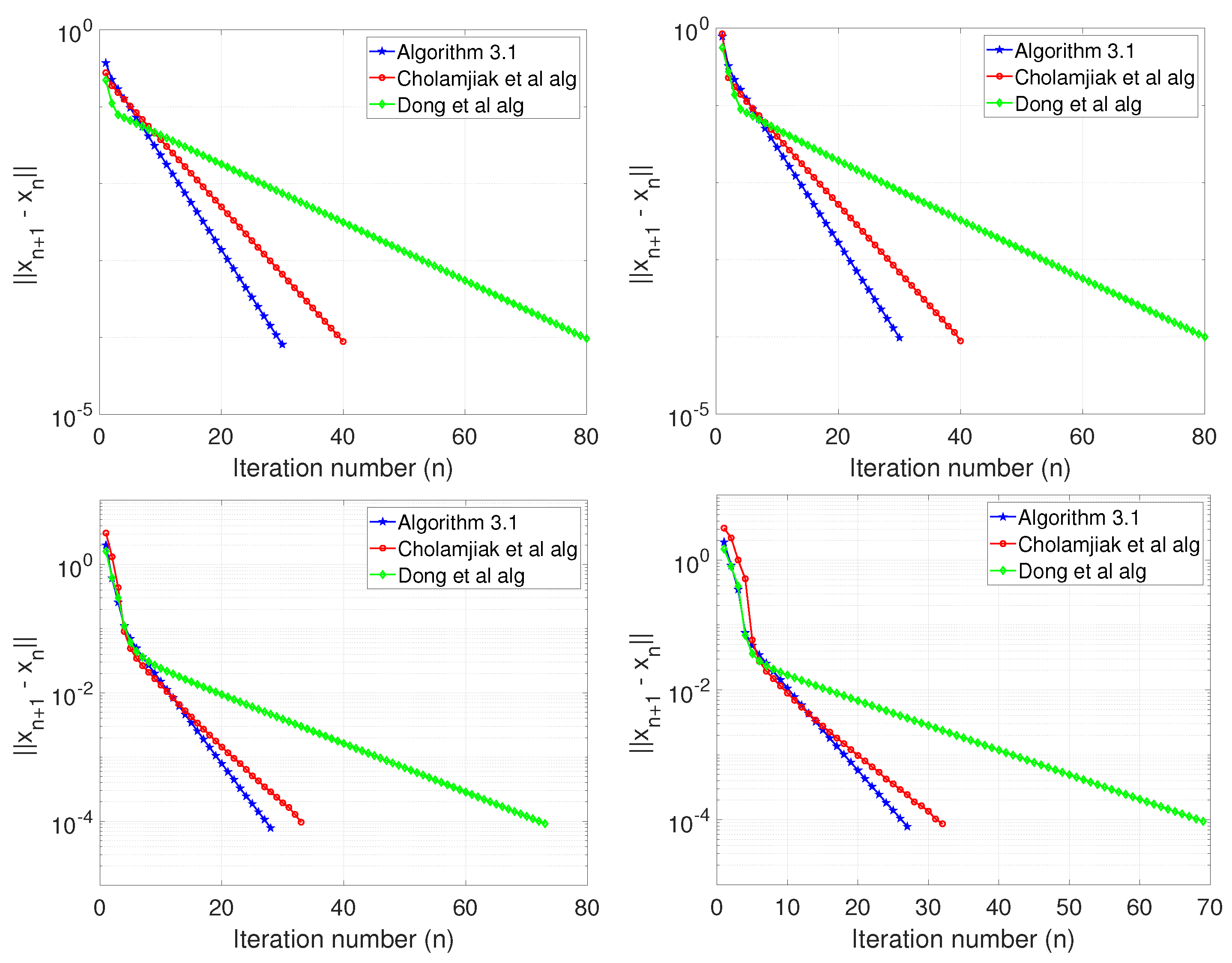
We take $T=U=P_{\mathsf{\Omega }}$ which is 0-demicontractive, $D=I,$ $f\left(x\right)=\frac{x}{2},$ $\forall x\in {\mathbb{R}}^N,$ $Bx=2x$ $\forall x\in {\mathbb{R}}^N,$ $\eta =1.99,$ $\rho =0.01,\vartheta =0.35,\alpha =0.0001,ϵ={10}^{-5},{\ell }_n=2,$ ${\delta }_n=\frac{1}{n+1},{\tau }_n=\frac{1}{{(n+1)}^2},$ ${\theta }_n=\frac{3n}{8n+3},$ ${\zeta }_n=\frac{1}{2}$ $\forall n\in \mathbb{N}.$ We compare the performance of our Algorithm 1 with Algorithm (5) of Cholamjiak et al. [27] and Algorithm (12) of Dong et al. [32]. In (5), we take ${\alpha }_n=\frac{1}{n+1},$ ${\theta }_n=\frac{1}{{(n+1)}^2},$ ${\delta }_n=\frac{3n}{8n+3},\beta =0.01,$ and $\eta =1.99.$ Also for (12), we choose ${\theta }_n=0.02,\beta =0.01,\eta =1.9,S=P_{\mathsf{\Omega }},{\alpha }_n=\frac{1}{n+1}.$ The computations were stopped when each algorithm satisfies $\parallel x_{n+1}-x_n\parallel <{10}^{-4}.$ The numerical results are shown in

Table 1. Computational result for Example 1.

		Algorithm 1	Cholamjiak et al. [27]	Dong et al. [32]
$N=5$	No of Iter.	30	40	80
	Time (sec)	0.0136	0.0181	0.0471
$N=10$	No of Iter.	30	40	80
	Time (sec)	0.0156	0.0195	0.0442
$N=30$	No of Iter.	28	33	73
	Time (sec)	0.0141	0.0172	0.0370
$N=50$	No of Iter.	27	32	69
	Time (sec)	0.0163	0.0201	0.0516

and Figure 1. In Figure 1, Algorithm 3.1 refers to Algorithm 1.

Example 2.

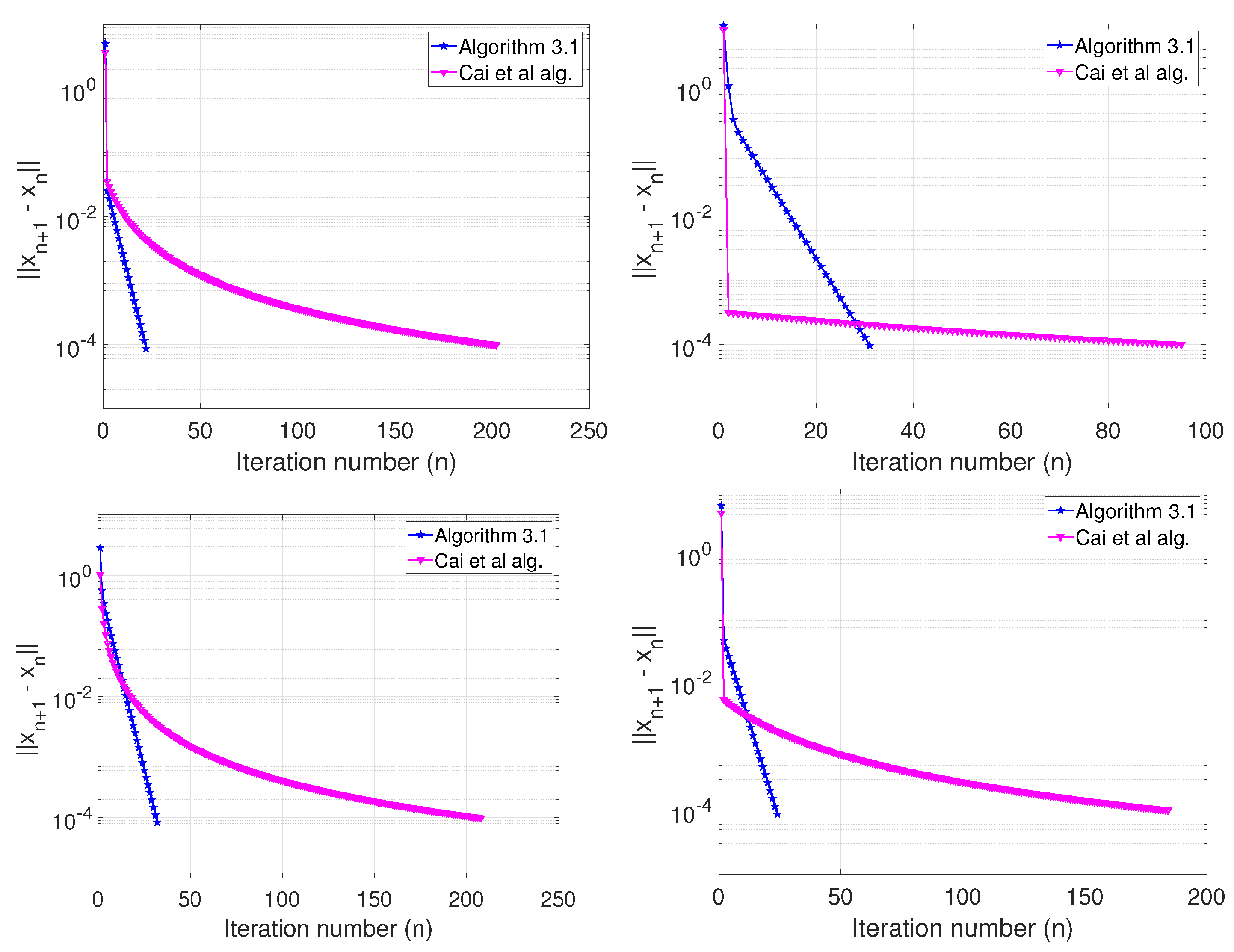
Next, we consider the min-max problem which can be formulated as a variational inequality problem with skew-symmetric matrix. This problem is to determine the shortest network in a given full Steiner topology (see (References [56], Example 1)). The compact form of the min-max problem is given as

$$\underset{x\in \mathcal{R}}{min}\underset{z\in \mathcal{B}}{max}{z}^T(Ax-b),$$

(67)

where

$$x^T={\left(x_{\left[1\right]}^T,\dots ,x_{\left[8\right]}^T\right)}^T,z^T={\left(z_{\left[1\right]}^T,\dots ,z_{\left[17\right]}^T\right)}^T,$$

$$\mathcal{R}={\mathbb{R}}^2\times \cdots \times {\mathbb{R}}^2\left(8times\right),\mathcal{B}=B_2,\dots ,B_2,\left(17times\right).$$

A is a block matrix of the form

$$A=\left(\begin{array}{cccc}{I}_2\hfill & \hfill & & \\ I_2\hfill & \hfill & & \\ \hfill & \ddots \hfill & \hfill & \\ \hfill & \hfill & \ddots \hfill & \\ \hfill & \hfill & & I_2\hfill \\ \hfill & \hfill & & I_2\hfill \\ I_2\hfill & -I_2\hfill & \hfill & \\ \hfill & \ddots \hfill & \ddots \hfill & \\ \hfill & \hfill & I_2\hfill & -I_2\hfill \end{array}\right)andb=\left(\begin{array}{c}{b}_{\left[1\right]}\hfill \\ b_{\left[2\right]}\hfill \\ ⋮\hfill \\ ⋮\hfill \\ b_{\left[9\right]}\hfill \\ b_{\left[10\right]}\hfill \\ 0\hfill \\ ⋮\hfill \\ 0\hfill \end{array}\right).$$

Equation (67) is equivalent to the following linear variational inequality (see References [15])

$$LVI(\mathsf{\Omega },M,q)u^{*}\in \mathsf{\Omega }{(u-u^{*})}^T(M{u}^{*}+q) \ge 0u\in \mathsf{\Omega },$$

(68)

where

$$u=\left(\begin{array}{c}{u}_1\hfill \\ u_2\hfill \end{array}\right),M=\left(\begin{array}{cc}0\hfill & A^T\hfill \\ -A\hfill & 0\hfill \end{array}\right),q=\left(\begin{array}{c}0\hfill \\ b\hfill \end{array}\right),and\mathsf{\Omega }=\mathcal{R}\times \mathcal{B}.$$

Note that M is skew-symmetric and the LVI is monotone. Also the mapping $Au=Mu+q$ in (68) is Lipschitz continuous. We set $B_2=\{x\in {\mathbb{R}}^2:\parallel x\parallel \le 1\}.$ We define the mapping $T:{\mathbb{R}}^2\to {\mathbb{R}}^2$ and $U:{\mathbb{R}}^2\to {\mathbb{R}}^2$ by

$$T(u_1,u_2)=\left\{\begin{array}{c}(u_1,u_2)if{u}_1<0,\hfill \\ (-2u_1,u_2)if{u}_1 \ge 0,\hfill \end{array}\right.$$

and

$$Ux=P_{\mathsf{\Delta }}\left(x\right)=\left\{\begin{array}{cc}d+r\frac{x-d}{\parallel x-d\parallel },\hfill & ifx\notin \mathsf{\Delta },\hfill \\ x,\hfill & ifx\in \mathsf{\Delta },\hfill \end{array}\right.$$

where Δ is the closed ball in ${\mathbb{R}}^2$ centered at $d\in {\mathbb{R}}^2$ with radius $r>0,$ that is, $\mathsf{\Delta }=\{x\in {\mathbb{R}}^2:\parallel x-d\parallel \le r\}.$ It is easy to see that T is $\frac{1}{3}$-demicontractive and not nonexpansive, while U is nonexpansive, and thus, $\frac{1}{3}$-demicontractive. We compare our method with the Projection contraction method of Cai et al. [15]. We take $\eta =1.78,\rho =0.02,\vartheta =0.67,\alpha =ϵ={10}^{-4},$ $l_n=5,$ ${\delta }_n=\frac{1}{{(n+1)}^{0.4}},$ ${\tau }_n={\delta }_n^2,$ ${\theta }_n=\frac{2n}{5n+7},$ ${\zeta }_n=0.45,$ $f\left(x\right)=\frac{x}{2},$ $Dx=x$ and choose the various initial values as follows:

Case I:

$x_0={[0,5]}^{\prime },x_1={\left[15\right]}^{\prime };$

Case II:

$x_0={[2,2]}^{\prime },x_1={[5,5]}^{\prime };$

Case III:

$x_0={[3,7]}^{\prime };x_1={[0,9]}^{\prime };$

Case IV:

$x_0={[1,8]}^{\prime },x_1={[3,4]}^{\prime }.$

For the Reference [15] algorithm, we used the Correction of PC Method 1 and take $\gamma =1.79.$ We used $\parallel x_{n+1}-x_n\parallel <{10}^{-4}$ as stopping criterion. The numerical results are shown in

Table 2. Computational result for Example 2.

		Algorithm 1	Cai et al. [15]
Case I	No of Iter.	22	202
	Time (sec)	0.0463	1.9129
Case II	No of Iter.	31	95
	Time (sec)	0.0097	0.0477
Case III	No of Iter.	32	208
	Time (sec)	0.0110	1.1696
Case IV	No of Iter.	24	184
	Time (sec)	0.0057	1.1250

and Figure 2.

Finally, we give an example in infinite dimensional spaces to support our strong convergence result.

Example 3.

Let $H_1=H_2=L^2\left([0,1]\right)$ with inner product $\langle x,y\rangle ={\int }_0^{1}x\left(t\right)y\left(t\right)dt$ and norm$\parallel x\parallel :={\left({\int }_0^1{\left|x\left(t\right)\right|}^{2}dt\right)}^{1/2},$$\forall x,y\in L^2\left([0,1]\right).$Let $\mathsf{\Omega }=\{x\in L^2\left([0,1]\right):\parallel x\parallel \le 1\}$ and $A:L^2\left([0,1]\right)\to L^2\left([0,1]\right)$ be given by $Ax\left(t\right)=max\{0,x(t\left)\right\}.$ Then A is monotone and uniformly continuous and

$$P_{\mathsf{\Omega }}\left(x\right)=\left\{\begin{array}{cc}\frac{x}{\parallel x\parallel }\hfill & if\parallel x\parallel >1,\hfill \\ x\hfill & if\parallel x\parallel \le 1.\hfill \end{array}\right.$$

We define the mapping $T=U={\int }_0^1\frac{x\left(t\right)}{2}dt,$ $t\in [0,1]$ and $x\in L^2\left([0,1]\right).$ Then $T=U$ is 0-demicontractive. We take $\eta =1.75, \vartheta =0.48, \rho =0.01, \alpha =ϵ={10}^{-3}, l_n=2,$ ${\delta }_n=\frac{1}{\sqrt{n+1}},$ ${\tau }_n=\frac{1}{n+1},$ ${\theta }_n=\frac{3n}{7n+9}, {\zeta }_n=\frac{2n}{5n+1}, f\left(x\right)=\frac{x}{2},$ $Dx=x.$ We also compare the performance of our Algorithm 1 with Algorithm (5) of Reference [27] and (12) of Reference [32]. For (5), we take $\eta =1.75, \beta =0.55, \theta ={10}^{-3}, {\alpha }_n=\frac{1}{\sqrt{n+1}},$ ${\tau }_n=\frac{1}{n+1}, {\delta }_n=\frac{2n}{5n+7}.$ Also for (12), we take $\eta =1.75, \beta =0.55 ,\theta =0.001, {\alpha }_n=\frac{1}{\sqrt{n+1}}.$ We test each algorithm using the following initial values and $\left|\right|x_{n+1}-x_n\left|\right|<{10}^{-5}$ as stopping criterion:

Case I:

$x_0=t^2-2t+3,x_1={(2t+1)}^3;$

Case II:

$x_0=exp\left(3t\right),x_1=sin\left(2t\right)/3;$

Case III:

$x_0=cos\left(5t\right)/10,x_1=sin\left(2t\right);$

Case IV:

$x_0=t^3+t-1,x_1=exp(-4t)/4.$

The numerical results are shown in

Table 3. Computational result for Example 3.

		Algorithm 1	Cholamjiak et al. [27]	Dong et al. [32]
Case I	No of Iter.	4	8	10
	Time (sec)	0.5669	0.9998	1.7530
Case II	No of Iter.	3	7	7
	Time (sec)	0.5101	0.6461	0.6706
Case III	No of Iter.	3	5	6
	Time (sec)	0.4019	0.5444	0.6242
Case IV	No of Iter.	3	4	5
	Time (sec)	0.2101	0.5938	0.7895

and Figure 3.

6. Conclusions

In this paper, we present a new generalized inertial viscosity approximation method for solving pseudomonotone variational inequality and split common fixed point problems in real Hilbert spaces. The algorithm is designed such that the stepsize of the variational inequality is determined by a line searching process and its convergence does not require norm of the bounded linear operator. A strong convergence result is proved under mild conditions and some numerical experiments are given to illustrate the efficiency and accuracy of the proposed method. This result improves and extends the results of References [16,17,18,26,27,32] and other related results in the literature.

References

- Alber, Y.; Ryazantseva, I. Nonlinear Ill-Posed Problems of Monotone Type; Springer: Dordrecht, The Netherlands, 2006. [Google Scholar]
- Bigi, G.; Castellani, M.; Pappalardo, M.; Passacantando, M. Nonlinear Programming Technique for Equilibria; Spinger Nature: Cham, Switzerland, 2019. [Google Scholar]
- Shehu, Y. Single projection algorithm for variational inequalities in Banach spaces with applications to contact problems. Acta Math. Sci. 2020, 40, 1045–1063. [Google Scholar] [CrossRef]
- Ceng, L.C.; Hadjisavas, N.; Weng, N.C. Strong convergence theorems by a hybrid extragradient-like approximation method for variational inequalities and fixed point problems. J. Glob. Optim. 2010, 46, 635–646. [Google Scholar] [CrossRef]
- Censor, Y.; Gibali, A.; Reich, S. Extensions of Korpelevich’s extragradient method for variational inequality problems in Euclidean space. Optimization 2012, 61, 119–1132. [Google Scholar] [CrossRef]
- Denisov, S.; Semenov, V.; Chabak, L. Convergence of the modified extragradient method for variational inequalities with non-Lipschitz operators. Cybern. Syst. Anal. 2015, 51, 757–765. [Google Scholar] [CrossRef]
- Fang, C.; Chen, S. Some extragradient algorithms for variational inequalities. In Advances in Variational and Hemivariational Inequalities; Springer: Cham, Switzerland, 2015; Volume 33, pp. 145–171. [Google Scholar]
- Hammad, H.A.; Ur-Rehman, H.; La Sen, M.D. Advanced algorithms and common solutions to variational inequalities. Symmetry 1198, 12, 1198. [Google Scholar] [CrossRef]
- Solodov, M.V.; Svaiter, B.F. A new projection method for variational inequality problems. SIAM J. Control Optim. 1999, 37, 765–776. [Google Scholar] [CrossRef]
- Censor, Y.; Gibali, A.; Reich, S. Strong convergence of subgradient extragradient methods for the variational inequality problem in Hilbert space. Optim. Methods Softw. 2011, 26, 827–845. [Google Scholar] [CrossRef]
- Censor, Y.; Gibali, A.; Reich, S. The subgradient extragradient method for solving variational inequalities in Hilbert spaces. J. Optim. Theory Appl. 2011, 148, 318–335. [Google Scholar] [CrossRef] [Green Version]
- Hieu, D.V. Parallel and cyclic hybrid subgradient extragradient methods for variational inequalities. Afr. Mat. 2017, 28, 677–679. [Google Scholar] [CrossRef]
- Jolaoso, L.O.; Taiwo, A.; Alakoya, T.O.; Mewomo, O.T. A self adaptive inertial subgradient extragradient algorithm for variational inequality and common fixed point of multivalued mappings in Hilbert spaces. Demonstr. Math. 2019, 52, 183–203. [Google Scholar] [CrossRef]
- Yang, J.; Liu, H. The subgradient extragradient method extended to pseudomonotone equilibrium problems and fixed point problems in Hilbert space. Optim. Lett. 2020, 14, 1803–1816. [Google Scholar] [CrossRef]
- Cai, X.; Gu, G.; He, B. On the O(1/t) convergence rate of the projection and contraction methods for variational inequalities with Lipschitz continuous monotone operators. Comput. Optim. Appl. 2014, 57, 339–363. [Google Scholar] [CrossRef]
- Jolaoso, L.O.; Taiwo, A.; Alakoya, T.O.; Mewomo, O.T. A unified algorithm for solving variational inequality and fixed point problems with application to the split equality problem. Comput. Appl. Math. 2019, 39. [Google Scholar] [CrossRef]
- Alakoya, T.O.; Jolaoso, L.O.; Mewomo, O.T. Modified inertial subgradient extragradient method with self-adaptive stepsize for solving monotone variational inequality and fixed point problems. Optimization 2020. [Google Scholar] [CrossRef]
- Thong, D.V.; Vinh, N.T.; Cho, Y.J. New strong convergence theorem of the inertial projection and contraction method for variational inequality problems. Numer. Algorithms 2020, 84, 285–305. [Google Scholar] [CrossRef]
- Jolaoso, L.O.; Aphane, M. Weak and strong convergence Bregman extragradient schemes for solving pseudo-monotone and non-Lipschitz variational inequalities. J. Ineq. Appl. 2020, 2020, 195. [Google Scholar] [CrossRef]
- Jolaoso, L.O.; Taiwo, A.; Alakoya, T.O.; Mewomo, O.T. A strong convergence theorem for solving pseudo-monotone variational inequalities using projection methods in a reflexive Banach space. J. Optim. Theory Appl. 2020, 185, 744–766. [Google Scholar] [CrossRef]
- Korpelevich, G.M. The extragradient method for finding saddle points and other problems. Ekon. Mat. Metody. 1976, 12, 747–756. (In Russian) [Google Scholar]
- Nadezhkina, N.; Takahashi, W. Weak convergence theorem by an extragradient method for nonexpansive mappings and monotone mappings. J. Optim. Theory Appl. 2006, 128, 191–201. [Google Scholar] [CrossRef]
- Vuong, P.T. On the weak convergence of the extragradient method for solving pseudo-monotone variational inequalities. J. Optim. Theory Appl. 2018, 176, 399–409. [Google Scholar] [CrossRef] [Green Version]
- He, B.S. A class of projection and contraction methods for monotone variational inequalities. Appl. Math. Optim. 1997, 35, 69–76. [Google Scholar] [CrossRef]
- Thong, D.V.; Hieu, D.V. Modified subgradient extragdradient algorithms for variational inequalities problems and fixed point algorithms. Optimization 2018, 67, 83–102. [Google Scholar] [CrossRef]
- Tian, M.; Jiang, B.N. Inertial hybrid algorithm for variational inequality problems in Hilbert spaces. J. Ineq. Appl. 2020, 2020, 12. [Google Scholar] [CrossRef] [Green Version]
- Cholamjiak, P.; Thong, D.V.; Cho, Y.J. A novel inertial projection and contraction method for solving pseudomonotone variational inequality problem. Acta Appl. Math. 2020, 169, 217–245. [Google Scholar] [CrossRef]
- Polyak, B.T. Some methods of speeding up the convergence of iteration methods. U.S.S.R. Comput. Math. Math. Phys. 1964, 4, 1–17. [Google Scholar] [CrossRef]
- Bot, R.I.; Csetnek, E.R.; Hendrich, C. Inertial Douglas-Rachford splitting for monotone inclusions. Appl. Math. Comput. 2015, 256, 472–487. [Google Scholar] [CrossRef] [Green Version]
- Chambole, A.; Dossal, C.H. On the convergence of the iterates of the “fast shrinkage/thresholding algorithm”. J. Optim. Theory Appl. 2015, 166, 968–982. [Google Scholar] [CrossRef]
- Dong, Q.-L.; Lu, Y.Y.; Yang, J. The extragradient algorithm with inertial effects for solving the variational inequality. Optimization 2016, 65, 2217–2226. [Google Scholar] [CrossRef]
- Dong, Q.L.; Cho, Y.J.; Zhong, L.L.; Rassias, T.M. Inertial projection and contraction algorithms for variational inequalites. J. Glob. Optim. 2018, 70, 687–704. [Google Scholar] [CrossRef]
- Jolaoso, L.O.; Alakoya, T.O.; Taiwo, A.; Mewomo, T.O. An inertial extragradient method via viscosity approximation approach for solving equilibrium problem in Hilbert spaces. Optimization 2020. [Google Scholar] [CrossRef]
- Jolaoso, L.O.; Oyewole, K.O.; Okeke, C.C.; Mewomo, O.T. A unified algorithm for solving split generalized mixed equilibrium problem and fixed point of nonspreading mapping in Hilbert space. Demonstr. Math. 2018, 51, 211–232. [Google Scholar] [CrossRef] [Green Version]
- Moudafi, A. Viscosity approximation method for fixed-points problems. J. Math. Anal. Appl. 2000, 241, 46–55. [Google Scholar] [CrossRef] [Green Version]
- Xu, H.K. Viscosity approximation method for nonexpansive mappings. J. Math. Anal. Appl. 2004, 298, 279–291. [Google Scholar] [CrossRef] [Green Version]
- Iiduka, H. Acceleration method for convex optimization over the fixed point set of a nonexpansive mappings. Math. Prog. Ser. A 2015, 149, 131–165. [Google Scholar] [CrossRef]
- Mainge, P.E. A hybrid extragradient viscosity method for monotone operators and fixed point problems. SIAM J. Control Optim. 2008, 49, 1499–1515. [Google Scholar] [CrossRef]
- Maingé, P.E. Projected subgradient techniques and viscosity methods for optimization with variational inequality constraints. Eur. J. Oper. Res. 2010, 205, 501–506. [Google Scholar] [CrossRef]
- Rudin, W. Functional Analysis, McGraw-Hill Series in Higher Mathematics; McGraw-Hill: New York, NY, USA, 1991. [Google Scholar]
- Marino, G.; Xu, H.K. Weak and strong convergence theorems for strict pseudo-contraction in Hilbert spaces. J. Math. Anal. Appl. 2007, 329, 336–346. [Google Scholar] [CrossRef] [Green Version]
- Maingé, P.E. Strong convergence of projected subgradient methods for nonsmooth and nonstrictly convex minimization. Set-Valued Anal. 2008, 16, 899–912. [Google Scholar] [CrossRef]
- Cottle, R.W.; Yao, J.C. Pseudo-monotone complementarity problems in Hilbert space. J. Optim. Theory Appl. 1992, 75, 281–295. [Google Scholar] [CrossRef]
- Yamada, I. The hybrid steepest-descent method for variational inequalities problems over the intersection of the fixed point sets of nonexpansive mappings. In Inherently Parallel Algorithms in Feasibility and Optimization and Their Applications; Butnariu, D., Censor, Y., Reich, S., Eds.; North-Holland: Amsterdam, The Netherlands, 2001; pp. 473–504. [Google Scholar]
- Maingé, P.E. Approximation methods for common fixed points of nonexpansive mappings in Hilbert spaces. J. Math. Anal. Appl. 2007, 325, 469–479. [Google Scholar] [CrossRef] [Green Version]
- Byrne, C. A unified treatment of some iterative algorithms in signal processing and image reconstruction. Inverse Probl. 2004, 20, 103–120. [Google Scholar] [CrossRef] [Green Version]
- Censor, Y.; Elfving, T. A multiprojection algorithm using Bregman projections in a product space. Numer. Alg. 1994, 8, 221–239. [Google Scholar] [CrossRef]
- Censor, Y.; Bortfeld, T.; Martin, B.; Trofimov, A.A. A unified approach for inversion problems in intensity-modulated radiation therapy. Phys. Med. Biol. 2006, 51, 2353–2365. [Google Scholar] [CrossRef] [Green Version]
- Censor, Y.; Elfving, T.; Kopf, N.; Bortfeld, T. The multiple-sets split feasibility problem and its applications for inverse problems. Inverse Probl. 2005, 21, 2071–2084. [Google Scholar] [CrossRef] [Green Version]
- Dong, Q.L.; Jiang, D.; Cholamjiak, P.; Shehu, Y. A strong convergence result involving an inertial forward-backward algorithm for monotone inclusions. J. Fixed Point Theory Appl. 2017, 19, 3097–3118. [Google Scholar] [CrossRef]
- Cholamjiak, P.; Suantai, S.; Sunthrayuth, P. Strong convergence of a general viscosity explicit rule for the sum of two monotone operators in Hilbert spaces. J. Appl. Anal. Comput. 2019, 9, 2137–2155. [Google Scholar] [CrossRef]
- Cholamjiak, P.; Suantai, S.; Sunthrayuth, P. An explicit parallel algorithm for solving variational inclusion problem and fixed point problem in Banach spaces. Banach J. Math. Anal. 2020, 14, 20–40. [Google Scholar] [CrossRef]
- Kesornprom, S.; Cholamjiak, P. Proximal type algorithms involving linesearch and inertial technique for split variational inclusion problem in hilbert spaces with applications. Optimization 2019, 68, 2365–2391. [Google Scholar] [CrossRef]
- Shehu, Y. On a modified extragradient method for variational inequality problem with application to industrial electricity production. J. Ind. Appl. Math. 2019, 15, 319–342. [Google Scholar]
- Yen, L.H.; Muu, L.D.; Huyen, N.T.T. An algorithm for a class of split feasibility problems: Application to a model in electricity production. Math. Meth. Oper. Res. 2016, 84, 549–565. [Google Scholar] [CrossRef]
- Xue, G.L.; Ye, Y.Y. An efficient algorithm for minimizing a sum of Euclidean norms with applications. SIAM J. Optim. 1997, 7, 1017–1036. [Google Scholar] [CrossRef] [Green Version]
Figure 1.
Example 1, Top Left: ; Top Right: ; Bottom Left: ; Bottom Right: .
Figure 2.
Example 2, Top Left: Case I; Top Right: Case II; Bottom Left: Case III; Bottom Right: Case IV.
Figure 3.
Example 3, Top Left: ; Top Right: ; Bottom Left: ; Bottom Right: .