A Fourth Order Energy Dissipative Scheme for a Traffic Flow Model

1
College of Liberal Arts and Sciences, National University of Defense Technology, Changsha 410073, China
2
State Key Laboratory of High Performance Computing, National University of Defense Technology, Changsha 410073, China
*
Author to whom correspondence should be addressed.
Mathematics 2020, 8(8), 1238; https://doi.org/10.3390/math8081238
Submission received: 24 June 2020
/
Revised: 19 July 2020
/
Accepted: 23 July 2020
/
Published: 28 July 2020
Abstract
:We propose, analyze and numerically validate a new energy dissipative scheme for the Ginzburg–Landau equation by using the invariant energy quadratization approach. First, the Ginzburg–Landau equation is transformed into an equivalent formulation which possesses the quadratic energy dissipation law. After the space-discretization of the Fourier pseudo-spectral method, the semi-discrete system is proved to be energy dissipative. Using diagonally implicit Runge–Kutta scheme, the semi-discrete system is integrated in the time direction. Then the presented full-discrete scheme preserves the energy dissipation, which is beneficial to the numerical stability in long-time simulations. Several numerical experiments are provided to illustrate the effectiveness of the proposed scheme and verify the theoretical analysis.
1. Introduction
The Ginzburg–Landau equation (GLE) was first proposed by Ginzburg and Landau in 1950 and applied to model the electrodynamics, quantum mechanics and thermodynamic properties of superconductors. As a state transformation equation, the GLE is closely related to many other state transformation equations, such as Allen–Cahn equation and Chafee–Infante equation. As is well known, the GLE plays an important role in the study of state transformation and unstable wave theory. Moreover, it has been widely used in optical fiber communication. In this paper, we consider the one-dimensional GLE as a model for traffic flow [1]
subject to the initial and boundary conditions
where and is the bounded domain. We denote the inner product by , the norm . Under the periodic boundary conditions, the global energy of the GLE is
where . Then the GLE in [1] can be rewritten as
Taking the inner product of the Equation (2) with m and the Equation (3) with , we obtain
Obviously, the GLE satisfies the energy dissipation law.
In recent years, many researchers have conducted various works about the GLE. Celledoni [1] proved that the average vector field (AVF) method can keep the energy dissipation of the Equation (1). The time-dependent GLE for the car traffic model is derived by Nagatani [2] through the perturbation method. Gunzburger and Hou [3] solved a series of problems for a Ginzburg–Landau model of superconductivity. They proposed finite element approximations for the optimality system and derived corresponding error estimates. The local well-posedness of the initial-boundary value problem for the complex GLE in bounded domains is investigated by Kuroda and Takanori [4]. Meanwhile, there are many effective ways to solve the GLE, such as the discontinuous Galerkin method [5], the semi-implicit method [6] and the trial equation method [7]. In addition, there also exist relevant studies on the fractional GLE [8,9,10,11] and the stochastic GLE [12,13,14,15,16]. However, most of previous researches can only achieve second order accuracy in the time direction. Therefore, the main challenge issue is to construct a high order energy dissipative scheme for the GLE.
The invariant energy quadratization (IEQ) approach [17] is a new method developed in recent years by introducing a Lagrange multiplier and has been successfully applied to a variety of gradient flow models [18,19,20,21,22,23,24]. By introducing a Lagrange multiplier and converting the nonlinear part to a semi-implicit scheme, a new linear system consisting of two coupled equations is calculated at each time step. A time-discretization scheme for the linear systems is constructed by Yang [25], which is easy to implement and achieve unconditionally energy stability. Liu [26] applyed two novel and efficient modified techniques based on IEQ approach to deal with nonlinear terms in gradient flows which succeeded in finding suitable positive preserving functions. Two linear and second order schemes that combine the IEQ approach with the stabilization technique are developed by Xu [27], where several extra linear stabilization terms are added and they are crucial to suppress the non-physical spatial oscillations caused by the strong anisotropy. Gong [28] presented a novel class of arbitrarily high-order and unconditionally energy-stable algorithms for gradient flow models by combining the IEQ approach and a specific class of Runge–Kutta (RK) methods. Since the solution to the Ginzburg–Landau equation shows instability very soon and this high order implicit scheme can unconditionally keep Ginzburg–Landau equation energy dissipation, we adopt this method to solve the Ginzburg–Landau equation. Ref. [28] combines IEQ approach and RK method and apply them to Cahn–Hilliard equation and Allen–Cahn equation to get the arbitrarily high-order schemes, while we apply it to the Ginzburg–Landau equation to construct a fourth order scheme in this paper.
The rest of this paper is organized as follows. In Section 2, the IEQ approach is introduced and applied to the GLE. Then the GLE is reformulated as a new system which admits a quadratic energy dissipation law. In Section 3, the Fourier pseudo-spectral method is used to obtain the semi-discrete the system of the GLE. After that, the implicit fourth order Runge–Kutta (RK4) method is applied for the time discretization to structure a full-discrete scheme. It is proved that the scheme we proposed is energy dissipative. In Section 4, the stability of the proposed scheme is verified by numerical experiments. We make a summary of this work in Section 5.
2. Invariant Energy Quadratization Approach
In this section, we present a new scheme for the GLE to preserve the energy dissipation law. By using the IEQ approach, we transform the Hamlitonian functional into a quadratic functional. We first introduce a Lagrange multiplier , then the GLE is transformed into
Theorem 1.
The system above preserves the energy dissipation law
where
3. High Order Energy Dissipative Scheme
3.1. Spatial Discretization by Using Fourier Pseudo-Spectral Method
In this part, we choose the Fourier pseudo-spectral method to discretize the system (4). It is proved that the semi-discrete scheme for the GLE preserves the semi-discrete energy dissipation law.
We primarily divide the domain into N equal intervals, where N is an even number. Afterwards, denote as the spatial step and as the grid points. The kth-order partial differential optrator can be approximated by the Fourier spectral differential matrix
where , . Clearly, is an skew-symmetric matrix.
By applying Fourier pseudo-spectral method to the system (4), we acquire the semi-discrete scheme
where , and .
Theorem 2.
The system (11) preserves the semi-discrete energy dissipation law
where
Proof.
The system (11) can be rewritten as follows
Taking the inner products of the system (12) with , and , respectively, we obtain the following semi-discrete energy dissipation law
□
It is known that the Equation (13) is equivalent to
where
is a symmetric and constant matrix.
3.2. Full Discretization by Using Implicit High Order Runge–Kutta Method
In previous studies, many methods have been proposed to solve energy dissipation system, such as the second order backward differentiation formula (BDF2), the AVF method and the backward Euler method. However, these methods can only structure first or second order energy dissipative schemes in the time direction meanwhile these schemes always require a lot of iterative computations, which not only affect the efficiency, but also bring cumulative errors in the calculation processes. Therefore, we propose a new scheme to acquire high order energy dissipative schemes for the GLE.
Let be real numbers and . For given , when an s-stage RK method is applied to the Equation (1), the following intermediate values are first calculated by
where . Then the high order energy dissipation scheme of the GLE is updated via
Proposition 1.
The RK coefficients are commonly displayed by a Butcher table
where , and with .
| c | A | ||
| = | |||
| ⋯ | |||
| ⋮ | ⋮ | ⋮ | |
| ⋯ | |||
| ⋯ | |||
In consequence, we choose RK(4,4) as
where , , , .
Definition 1.
Let be a symmetric, constant matrix. For a dissipative system, the RK method defined by the Butcher array is said to be -dissipative if applid to the new system (15)
for all and for all .
Theorem 3.
([29]) A RK scheme defined by the Butcher array is said to be -dissipative, if and only if the symmetric coefficient matrix M with elements
are nonnegative.
Proof.
Above all, replace by the new system (15), that can be derived as
Substituting into the first term on the right hand side of the Equation (17), we get
Whereafter, it can be arranged as
Noticing that and , we have
This completes the proof. □
In this paper, we only consider four stage and fourth order diagonally implicit RK scheme, which belongs to -dissipative RK scheme can be extended to higher order RK method without any necessary difficulties.
4. Numerical Simulation
In this section, we carry out two numerical experiments by applying the implicit high order energy dissipative scheme. The stability and the convergence of the new scheme (15) are verified by these numerical experiments. Meanwhile, we compare the proposed scheme (15) with the AVF method in energy errors and accuracy. The numerical iteration formula of the AVF method is
where . In the following text, the Newton iteration is mainly used to solve the full-discrete system.
Example 1.
We utilize the initial condition of single solitary wave given by
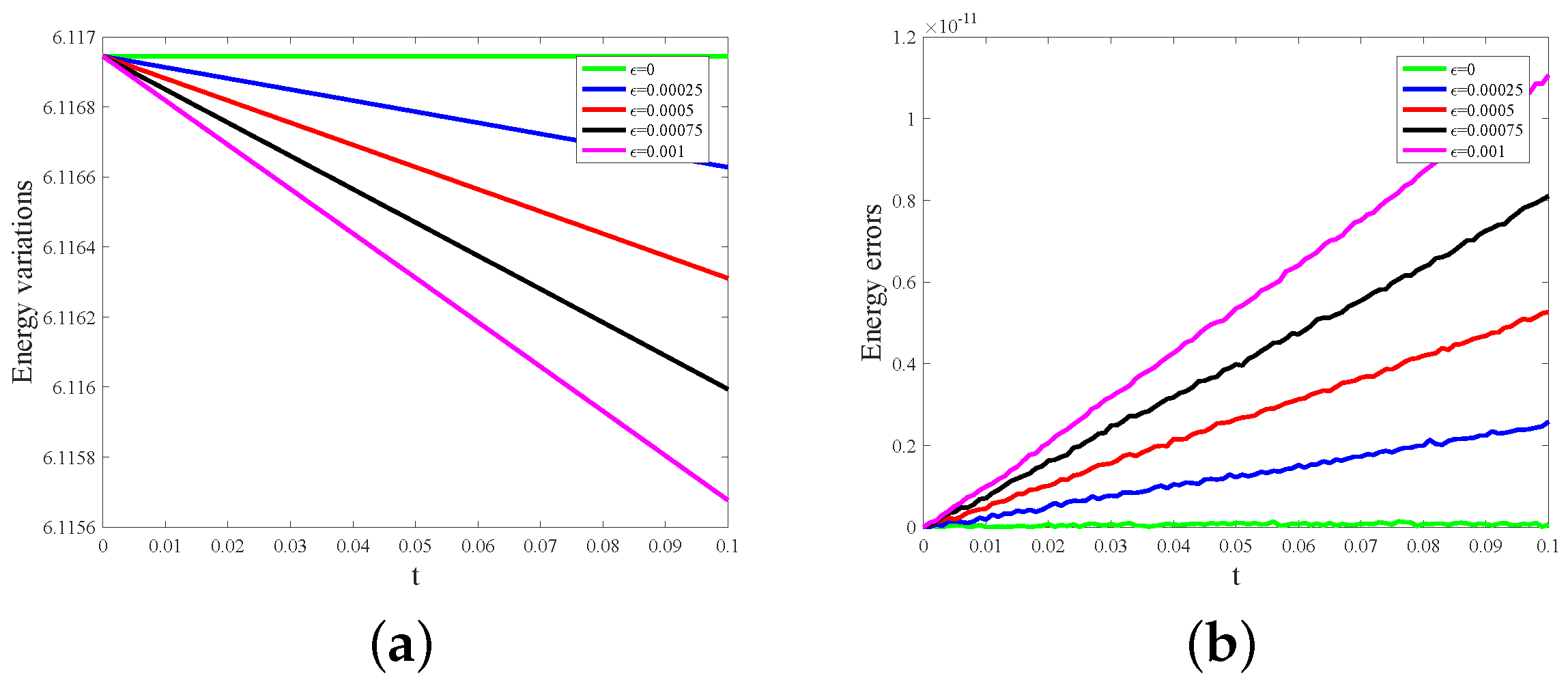
to observe how the coefficient ϵ affects the energy dissipation. First, we set , the number of grid points and the time step . Letting respectively, the energy variations and energy errors of the proposed scheme (15) are presented in Figure 1. Based on Figure 1a, we find the proposed scheme (15) can preserve the discrete energy conservation exactly when , and the energy dissipations of the GLE can be observed when . Obviously, with bigger ϵ, the energy dissipates faster. Taking the discrete energy obtained from the scheme (15) with and as the reference discrete energy, we plot the energy errors () with various ε in Figure 1b. It shows that the proposed new scheme (15) can preserve the energy dissipation of the GLE. Meanwhile, Figure 1b indicates that the energy dissipation is a little bit influenced by the time step size. The waveforms, energy variations and energy errors obtained from the scheme (15) and the scheme (18) with , , are pictured in Figure 2. The waveforms obtained from these two schemes at are almost the same (Figure 2a). Figure 2b shows that they both can keep the energy reducing steadily. According to Figure 2c, comparatively speaking, the energy errors obtained by the proposed scheme (15) is even smaller than that by the scheme (18).
Setting and , we list the convergence rates of the proposed new scheme (15) in Table 1 and Table 2. For the time accuracy test, we select the numerical solution with and as the reference solution. Based on Table 1, the convergence order of the proposed scheme (15) in time is 4 and the scheme (18) only converges with second-order accuracy. For the space accuracy test, the scheme (15) and the scheme (18) both apply the Fourier pseudo-spectral method in space-discretization, thus the space convergence orders of them decrease in an exponential rate in Table 2 (the numerical solution with and is chosen as the reference solution).
Example 2.
In the second example, we investigate the energy dissipation of double solitary wave with the initial condition,
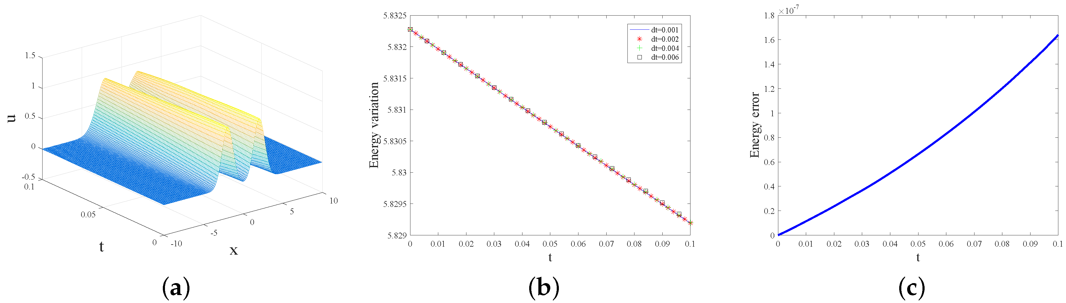
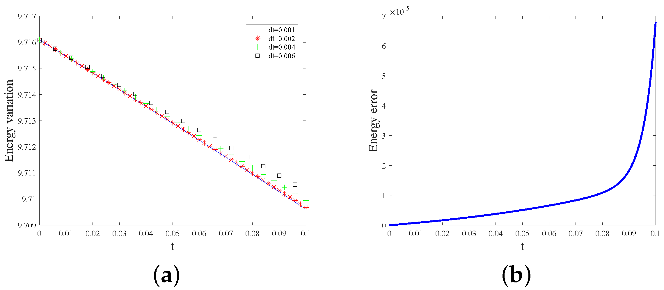
By setting and , we plot the waveform of double solitary wave with and in Figure 3a. The energy dissipation property of the GLE with various time steps can be verified in Figure 3b. It shows the new scheme (15) can keep energy dissipation at a large time step. Taking the discrete energy obtained from the new scheme (15) with as the reference discrete energy, the energy error in Figure 3c is only about . Then using the same grid, we consider the situation of and and plot the energy variation and the energy error in Figure 4. As we can see, the proposed scheme (15) still can maintain the energy dissipation property with various time steps.
5. Conclusions
In this paper, we have developed a stable and high order energy dissipative scheme for solving the GLE. By using the IEQ approach, the GLE is downgraded from fourth order to second order. The full-discrete system of GLE is obtained by using the Fourier pseudo-spectral method in the spatial direction and the diagonally implicit Runge–Kutta method in the time direction. The new scheme (15) we proposed has three main advantages. First of all, it is well-known that the implicit methods enjoy better stability in the simulation of stiff equations. Besides, it has high calculation efficiency due to the application of the diagonally implicit Runge–Kutta method. Last but not least, the high order scheme in time direction can be constructed and the energy dissipation can be preserved. The proposed implicit fourth order scheme can maintain the energy dissipation of the GLE theoretically. Moreover, the numerical results of single solitary wave and double solitary wave have verified the stability and accuracy of the proposed scheme. Compared with the scheme (18), the proposed scheme converges with fourth order in the time direction and can be generalized to construct higher order energy dissipative scheme naturally.
Author Contributions
Conceptualization, X.C.; Project administration, S.S.; Writing—original draft, X.C.; Writing—review editing, M.S. All authors have read and agreed to the published version of the manuscript.
Funding
This research was funded by National Natural Science Foundation of China (Grant No. 11901577 11971481) and the National Natural Science Foundation of Hunan (Grant No. S2017JJQNJJ0764), Research Fund of National University of Defense Technology (Grant No. ZK17-03-27), and the fund from Hunan Provincial Key Laboratory of Mathematical Modeling and Analysis in Engineering (Grant No. 2018MMAEZD004).
Conflicts of Interest
The authors declare no conflict of interest.
References
- Celledoni, E.; Grimm, V.; McLachlan, R.I.; McLaren, D.I.; O’Neale, D.; Owren, B.; Quispel, G.R.W. Preserving energy resp. dissipation in numerical PDEs using the “Average Vector Field” method. J. Comput. Phys. 2012, 231, 6770–6789. [Google Scholar] [CrossRef] [Green Version]
- Nagatani, T. Time-dependent Ginzburg–Landau equation for the jamming transition in traffic flow. Phys. Stat. Mech. Appl. 1998, 258, 237–242. [Google Scholar] [CrossRef]
- Gunzburger, M.D.; Hou, L.S.; Ravindran, S.S. Analysis and approximation of optimal control problems for a simplified Ginzburg–Landau model of superconductivity. Numer. Math. 1997, 77, 243–268. [Google Scholar] [CrossRef]
- Kuroda, T.; Ôtani, M. Local well-posedness of the complex Ginzburg–Landau equation in bounded domains. Nonlinear Anal. Real World Appl. 2019, 45, 877–894. [Google Scholar] [CrossRef] [Green Version]
- Yildiz, T.A.; Uzunca, M.; Karasozen, B. Structure preserving reduced order modeling for gradient systems. Appl. Math. Comput. 2019, 347, 194–209. [Google Scholar]
- Chen, L.Q.; Shen, J. Applications of semi-implicit Fourier-spectral method to phase field equations. Comput. Phys. Commun. 1998, 108, 147–158. [Google Scholar] [CrossRef]
- Liu, Y.; Chen, S.Q.; Wei, L.X.; Guan, B. Exact solutions to complex Ginzburg–Landau equation. Pramana J. Phys. 2018, 91. [Google Scholar] [CrossRef]
- Zhang, Q.G.; Li, Y.N.; Su, M.L. The local and global existence of solutions for a time fractional complex Ginzburg–Landau equation. J. Math. Anal. Appl. 2019, 469, 16–43. [Google Scholar] [CrossRef]
- He, D.D.; Pan, K.J. An unconditionally stable linearized difference scheme for the fractional Ginzburg–Landau equation. Numer. Algorithms 2018, 79, 899–925. [Google Scholar] [CrossRef]
- Li, L.; Jin, L.Y.; Fang, S.M. Large time behavior for the fractional Ginzburg–Landau equations near the BCS-BEC crossover regime of Fermi gases. Bound. Value Probl. 2017, 2017, 8. [Google Scholar] [CrossRef] [Green Version]
- Lu, H.; Bates, P.W.; Lu, S.J.; Zhang, M.J. Dynamics of the 3D fractional Ginzburg–Landau equation with multiplicative noise on an unbounded domain. Commun. Math. Sci. 2016, 14, 273–295. [Google Scholar] [CrossRef]
- Guo, Y.F.; Li, D.L. Random attractor stochastic complex Ginzburg–Landau equation with multiplicative noise ou unbounded domain. Stoch. Anal. Appl. 2017, 35, 409–422. [Google Scholar] [CrossRef]
- Shen, T.L.; Huang, J.H. Ergodicity of 2D stochastic Ginzburg–Landau-Newell equations driven by degenerate noise. Math. Method Appl. Sci. 2017, 40, 4812–4831. [Google Scholar]
- Shen, T.L.; Xin, J.; Huang, J.H. Time-space fractional stochastic Ginzburg–Landau equation driven by Gaussian white noise. Stoch. Anal. Appl. 2018, 36, 103–113. [Google Scholar] [CrossRef]
- Chugreeva, O.; Melcher, C. Vortices in a stochastic parabolic Ginzburg–Landau equation. Stochastics Partial. Differ. Equations Anal. Comput. 2017, 5, 113–143. [Google Scholar] [CrossRef] [Green Version]
- Lin, L.; Gao, H.J. A stochastic generalized Ginzburg–Landau equation driven by jump noise. J. Theor. Probab. 2019, 32, 460–483. [Google Scholar] [CrossRef] [Green Version]
- Guillen, G.F.; Tierra, G. On linear schemes for a Cahn-Hilliard diffuse interface model. J. Comput. Phys. 2013, 234, 140–171. [Google Scholar] [CrossRef]
- Han, D.Z.; Brylev, A.; Yang, X.F.; Tan, Z.J. Numerical analysis of second order, fully discrete energy stable schemes for phase field models of two-phase incompressible flows. J. Sci. Comput. 2017, 70, 965–989. [Google Scholar] [CrossRef]
- Zhao, J.; Yang, X.F.; Gong, Y.Z.; Wang, Q. A novel linear second order unconditionally energy stable scheme for a hydrodynamic q-tensor model of liquid crystals. Comput. Method Appl. Mech. Eng. 2017, 318, 803–825. [Google Scholar] [CrossRef] [Green Version]
- Yang, X.F. Linear, first and second-order, unconditionally energy stable numerical schemes for the phase field model of homopolymer blends. J. Comput. Phys. 2016, 327, 294–316. [Google Scholar] [CrossRef] [Green Version]
- Yang, X.F.; Han, D.Z. Linearly first and second-order, unconditionally energy stable schemes for the phase field crystal model. J. Comput. Phys. 2017, 33, 1116–1134. [Google Scholar] [CrossRef] [Green Version]
- Yang, X.F.; Ju, L.L. Efficient linear schemes with unconditional energy stability for the phase field elastic bending energy model. Comput. Method Appl. Mech. Eng. 2017, 315, 691–712. [Google Scholar] [CrossRef] [Green Version]
- Yang, X.F.; Ju, L.L. Linear and unconditionally energy stable schemes for the binary fluid-surfactant phase field model. Comput. Method Appl. Mech. Eng. 2017, 318, 1005–1029. [Google Scholar] [CrossRef] [Green Version]
- Yang, X.F.; Zhao, J.; Wang, Q. Numerical approximations for the molecular beam epitaxial growth model based on the invariant energy quadratization method. J. Comput. Phys. 2017, 333, 104–127. [Google Scholar] [CrossRef] [Green Version]
- Yang, X.F.; Zhao, J.; Wang, Q.; Shen, J. Numerical approximations for a three-component Cahn-Hilliard phase-field model based on the invariant energy quadratization method. Math. Model. Methods Appl. Sci. 2017, 27, 1993–2030. [Google Scholar] [CrossRef]
- Liu, Z.G.; Li, X.L. Efficient modified techniques of invariant energy quadratization approach for gradient flows. Appl. Math. Lett. 2019, 98, 206–214. [Google Scholar] [CrossRef]
- Xu, Z.; Yang, X.F.; Zhang, H.; Xie, Z.Q. Efficient and linear schemes for anisotropic Cahn-Hilliard model using the Stabilized-Invariant Energy Quadratization (S-IEQ) approach. Comput. Phys. Commun. 2019, 238, 36–49. [Google Scholar] [CrossRef]
- Gong, Y.Z.; Zhao, J. Energy-stable Runge–Kutta schemes for gradient flow models using the energy quadratization approach. Appl. Math. Lett. 2019, 94, 224–231. [Google Scholar] [CrossRef]
- Buono, N.D.; Mastroserio, C. Explicit methods based on a class of four stage fourth order Runge–Kutta methods for preserving quadratic laws. J. Comput. Appl. Math. 2002, 140, 231–243. [Google Scholar] [CrossRef] [Green Version]
Figure 1.
The energy variations (a) and energy errors (b) of the scheme (15) with various .

Figure 2.
The waveforms (a), energy variationas (b) and energy errors (c) of the scheme (15) and the scheme (18).
Figure 2.
The waveforms (a), energy variationas (b) and energy errors (c) of the scheme (15) and the scheme (18).

Figure 3.
The waveform (a), energy variation (b) and energy error (c) of the scheme (15) at with and .
Figure 3.
The waveform (a), energy variation (b) and energy error (c) of the scheme (15) at with and .

Figure 4.
The energy variation (a) and energy error (b) of the scheme (15) at with and .


Table 1.
Time accuracy test for the scheme (15) and the scheme (18) at .
| t | New Scheme (15) | Time Order | Scheme (18) | Time Order |
|---|---|---|---|---|
| 0.002 | - | - | ||
| 0.001 | 3.994 | 2.016 | ||
| 0.0005 | 3.999 | 2.044 | ||
| 0.00025 | 4.000 | 2.193 |
Table 2.
Space accuracy test for the scheme (15) and the scheme (18) at .
| N | New Scheme (15) | Space Order | Scheme (18) | Space Order |
|---|---|---|---|---|
| 10 | - | - | ||
| 20 | 0.994 | 1.844 | ||
| 40 | 10.253 | 9.794 | ||
| 80 | 15.533 | 15.978 |
© 2020 by the authors. Licensee MDPI, Basel, Switzerland. This article is an open access article distributed under the terms and conditions of the Creative Commons Attribution (CC BY) license (http://creativecommons.org/licenses/by/4.0/).
Share and Cite
MDPI and ACS Style
Chen, X.; Song, M.; Song, S. A Fourth Order Energy Dissipative Scheme for a Traffic Flow Model. Mathematics 2020, 8, 1238. https://doi.org/10.3390/math8081238
AMA Style
Chen X, Song M, Song S. A Fourth Order Energy Dissipative Scheme for a Traffic Flow Model. Mathematics. 2020; 8(8):1238. https://doi.org/10.3390/math8081238
Chicago/Turabian StyleChen, Xiaowei, Mingzhan Song, and Songhe Song. 2020. "A Fourth Order Energy Dissipative Scheme for a Traffic Flow Model" Mathematics 8, no. 8: 1238. https://doi.org/10.3390/math8081238
Note that from the first issue of 2016, this journal uses article numbers instead of page numbers. See further details here.