On the Fractional Wave Equation

Dipartimento di Scienze Statistiche, Sapienza, University of Rome, 00185 Rome, Italy
*
Author to whom correspondence should be addressed.
Mathematics 2020, 8(6), 874; https://doi.org/10.3390/math8060874
Submission received: 13 May 2020
/
Revised: 26 May 2020
/
Accepted: 27 May 2020
/
Published: 31 May 2020
(This article belongs to the Special Issue Stability Problems for Stochastic Models: Theory and Applications)
Abstract
:In this paper we study the time-fractional wave equation of order and give a probabilistic interpretation of its solution. In the case , , the solution can be interpreted as a time-changed Brownian motion, while for it coincides with the density of a symmetric stable process of order . We give here an interpretation of the fractional wave equation for in terms of laws of stable d−dimensional processes. We give a hint at the case of a fractional wave equation for and also at space-time fractional wave equations.
1. Introduction
In this paper we study in detail the solution of the time-fractional equation
for under the initial conditions
The time-fractional derivative is hereafter understood in the Caputo sense:
We first prove that the Fourier transform of the solution of the Cauchy problem (1) and (2) is
where
is the one-parameter Mittag-Leffler function, first introduced in [1]. The representation of (4) as a contour integral on the Hankel path
permits us to obtain a representation of (6) as
Some details about the representation (6) and the Hankel path can be found in [2]. For , the inversion of (7) is presented in [3] with the conclusion that the solution of (1) is the distribution of a stable symmetric process of order .
We here show that for , the solution can be expressed in terms of the law of a d−dimensional stable process with a suitable choice of the measure Γ appearing in
In particular, for Γ uniform on the upper and lower hemispheres of , we prove that (8) yields the characteristic functions in square brackets of Formula (7). We give also the explicit forms of of the solution of (1) in terms of Bessel functions , which for can be reduced to Fujita’s result. Some results concerning wave equations of fractional type can be found, e.g., in [4].
2. The Fractional Wave Equation
In this note we present some relationship between stable processes (and their inverses) with fractional equations. Stable processes are studied in depth in the monograph [5]. Some simple and well known results state that a symmetric stable process with characteristic function
has distribution , satisfying the fractional equation
where is the Riesz fractional derivative usually defined as
with Fourier transform
For the d-dimensional isotropic stable process with characteristic function,
The corresponding probability law satisfies the equation
where is the fractional Laplacian defined as the operator such that
where is the Fourier transform of a function and the domain of the operator is
(on this point see for example [6]). The connection between fractional operators and stochastic processes is explored, e.g., in [7]. A detailed comparison of the several possible definitions of the fractional Laplacian can be found in [8]. For the time-fractional equation (see [9]),
we have that the solution of the Cauchy problem is explicitly given by
where
is the Wright function. The d−dimensional counterpart of (16) is
Some details about time-fractional derivatives can be found in [10]. For the solution of (18) corresponds to the distribution of the vector process
where is the d−dimensional Brownian motion and is the inverse of the stable subordinator (see [11]).
In the more general case
The solution of the Cauchy problem (20) is the probability density of the process
where is an isotropic stable process (see [11]). We here consider the case where in (18) and (20) the order of the fractional derivative is .We start first with (18) and observe that the Laplace–Fourier transform of the solution is
and the Fourier transform reads
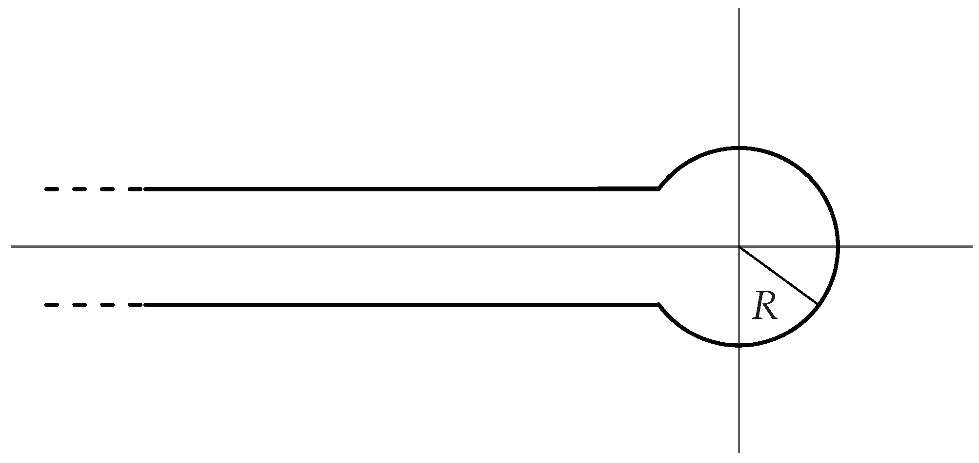
The Mittag-Leffler function can be represented as a contour integral on the Hankel path as
where is the contour in the complex plane represented in Figure 1.
The representation (24) is a consequence of the integral representation of the inverse of the Gamma function
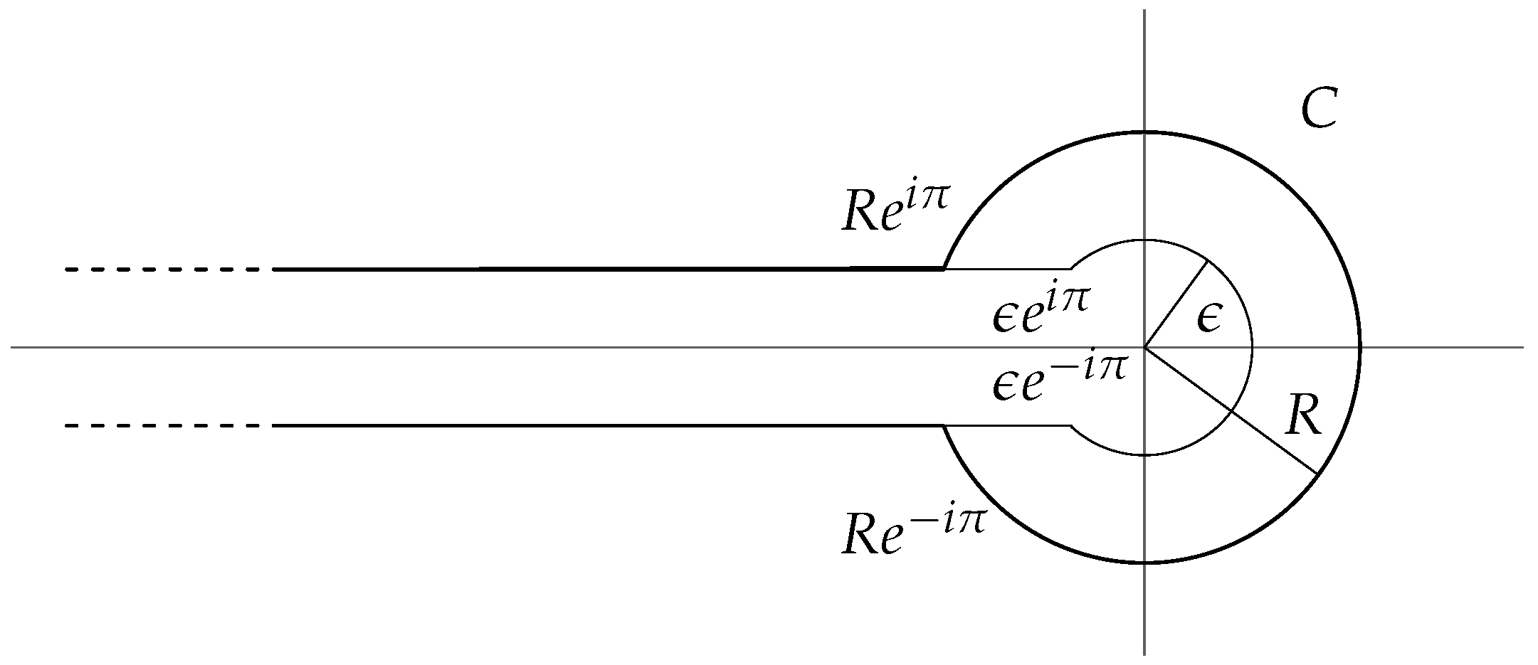
The integral in (24) can be developed by inserting a ring of radius .
The contour C is composed by the circumferences and with two segments joining with and with , and is run counterclockwise. See Figure 2.
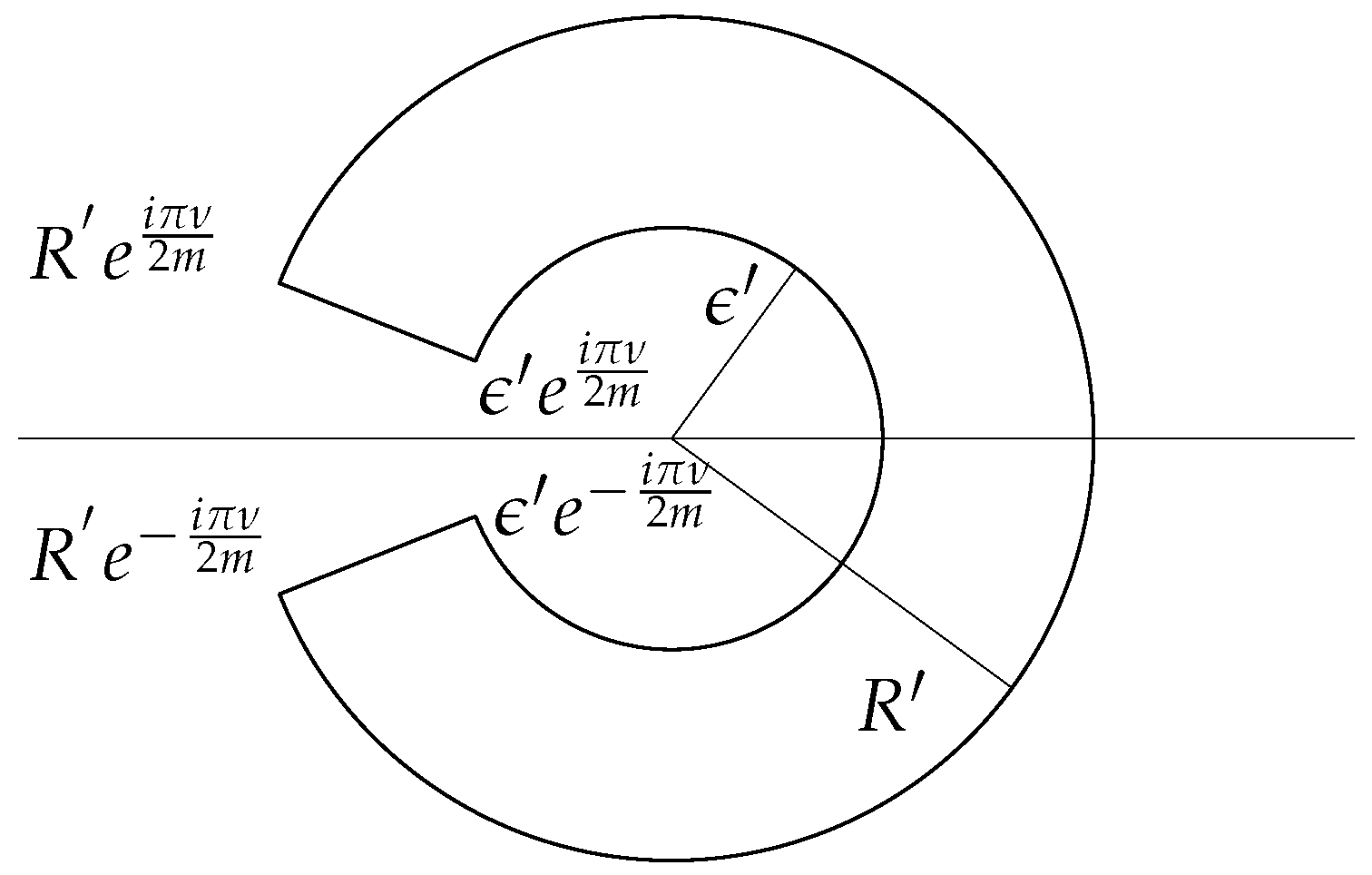
In order to evaluate
we perform the transformation for .
Therefore, the horizontal segments of Figure 2 are rotated by an angle of amplitude and the radii are subject to contraction or dilation according to the value of ν. The integral on thus obtained from (25) is
The integral on the right side of (26) can be evaluated by means of the Cauchy residue theorem. The function
has poles at points for . It is easy to show that the residues of (27) at the poles are given by
Thus the integral (26) can be written as
By adding the contribution of the segments and for and we obtain
For we must distinguish the cases where
and , where
In order to simplify the formulas involved in the analysis we take .
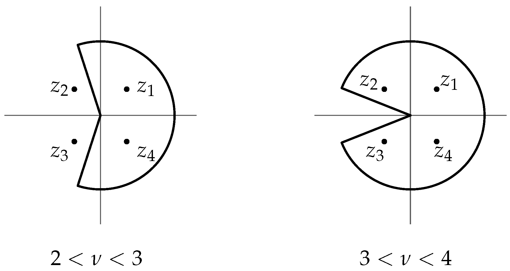
For we have the subcases and . In the first case the contour integral of Figure 3 involves two poles and thus yields two additional terms in the representation of the Mittag-Leffler function (32). In the second case we have the contribution of four poles in the contour integral of Figure 3, so that for
The contours for and are depicted below (Figure 4).
The substantial difference between the cases and is that in the first case we have that is negative and the contribution of the poles correspond to the characteristic function of stable processes, whereas for , and are positive and thus are not characteristic functions of random variables. Let us now concentrate our attention on the integrals in Equations (31) and (32) (which is also true in the general case for ). If we write
where W is a non-negative r.v. with density
Note that for the function (2) is negative on . We note also that the r.v. with density
appearing in (35) has the same distribution as the ratio of two independent stable subordinators of degree .
We now give the inverse Fourier transform of (34) for , .
We start by evaluating the following integral
where .
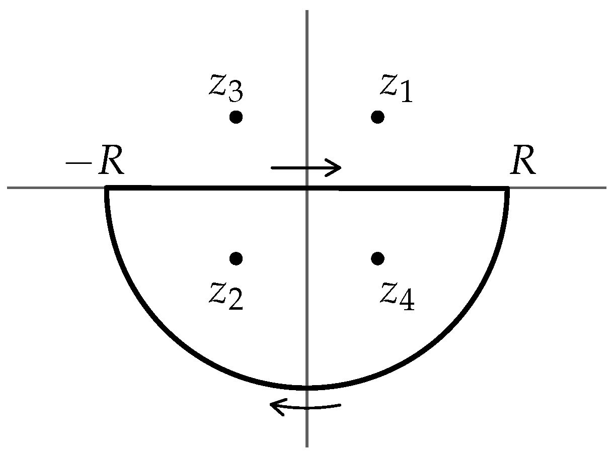
We must now evaluate the integral of
on a suitable contour . The four roots of are
and are located in C as in Figure 5, because .
We observe that for and , the curvilinear integral on the half-circle tends to zero as . By the residue theorem we thus have
The minus sign is due to the fact that the contour in Figure 5 is run clockwise.
The residues and have the following values
and thus
For , the integration of must be performed on the contour of Figure 6 and
the sign being in this case positive because the path is run counterclockwise.
The residues in this case are
The integral (40), therefore, takes the form
In conclusion we have that
We now consider the integration with respect to w in (36). This leads to the evaluation of the following integral
The last step of (43) can be developed as follows
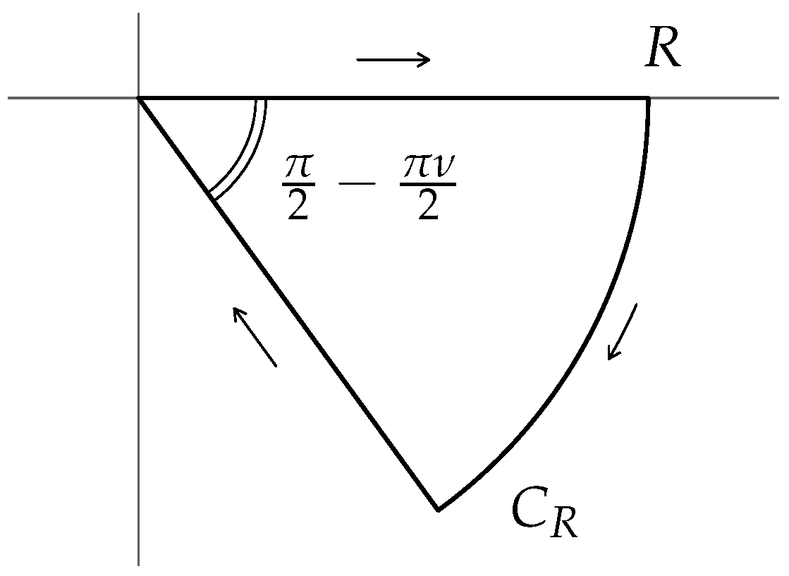
We evaluate the first integral in (44) by taking the contour integral of the function
along the path depicted in Figure 7.
By the Cauchy theorem we have that
The integral on the arc C tends to zero because
Since as , the exponent of the second factor of (46) is negative as well as the first one because for θ ranging in the same interval.
From (32), , we conclude that
Remark 1.
The function is the characteristic function of a stable random variable of order with symmetry parameter . Many details about the properties of such densities can be found in [12]. The function is unimodal with a positive maximal point and is such that . Analogously, the function is the characteristic function of a negatively skewed random variable. This implies that the function can be seen as the superposition of the densities of stable random variables with index , conditional to be respectively positive or negative.
3. The Multidimensional Case for
The Cauchy problem
has solution with Fourier transform
as shown in the analysis presented above. Thus, the solution to the Cauchy problem (50) reads
We must therefore evaluate the following three d−dimensional integrals, the first one being a function of z.
Since the three integrals (53) are substantially similar, we restrict ourselves to the evaluation of the first one. In spherical coordinates we have that
The last step is the hyperspherical integral
which is proven in detail in [13], Formula (2.151).
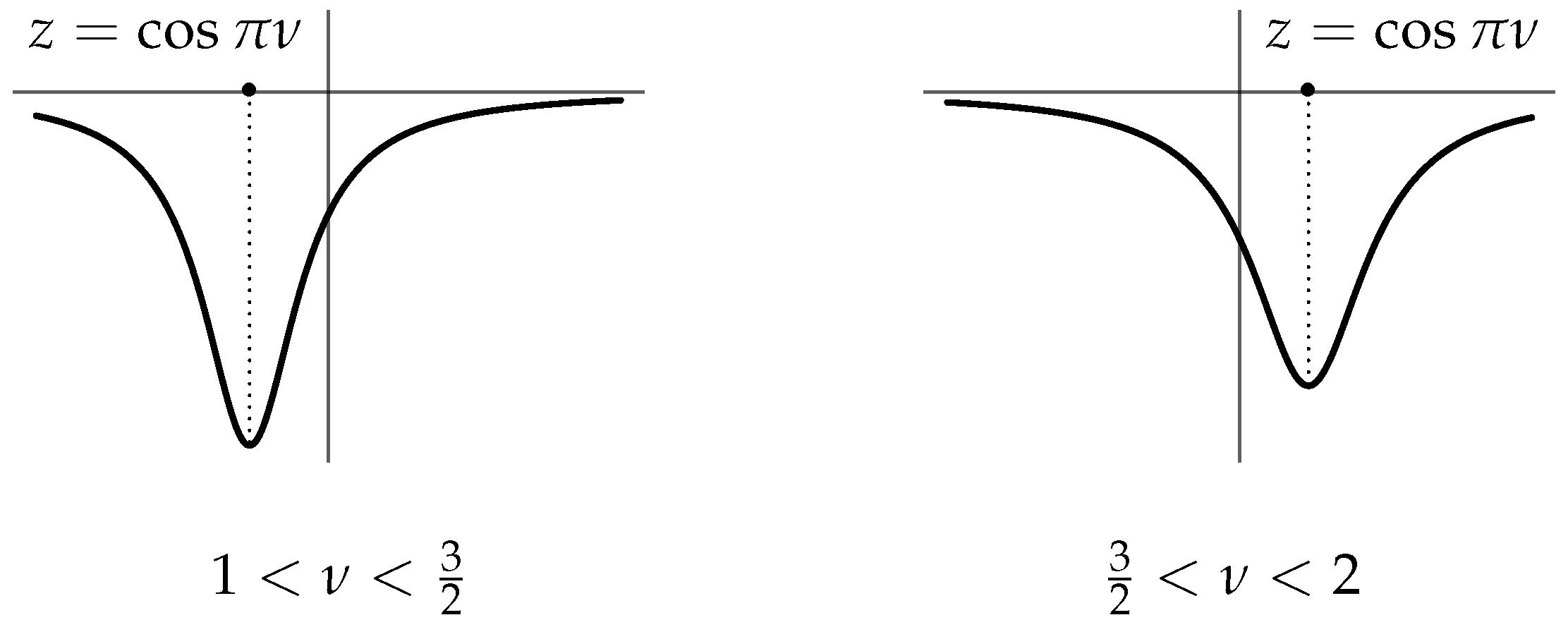
Note that the integral in z after the change of variable becomes
since the function
has the form shown in Figure 9.
In conclusion
We recall now the definition of an α−stable d−dimensional process , .
Its characteristic function has the following form [14]
where , Γ is a finite measure on the sphere .
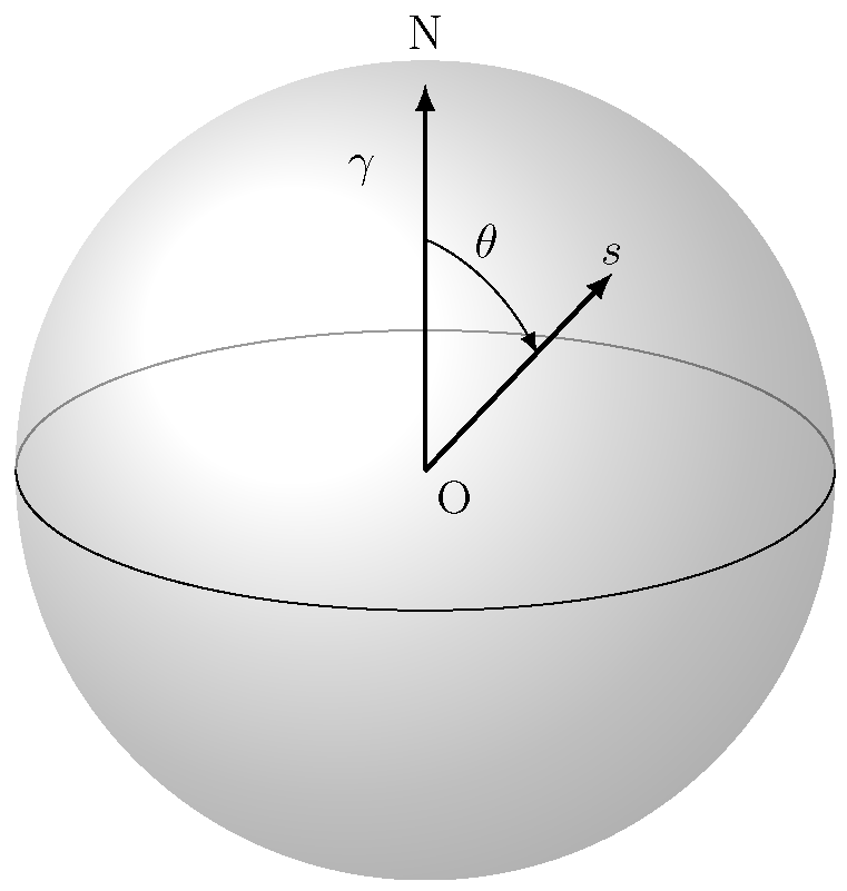
Since , where so that . Furthermore . We can assume γ oriented through the north pole of and thus θ can be viewed as the latitude of vector s, as shown in Figure 10.
We take the case and rewrite the characteristic function as
where .
For simplicity we assume and suppose that Γ is a uniformly distributed measure on the upper hemisphere of the unit sphere. Thus
with . For the integral in (61) becomes
The characteristic function (61) turns out to be
Since and , we have so is negative.
If Γ is distributed on the lower hemisphere , and in the same way we have that
The situation in the space , is quite similar with the integral in (61) evaluated in hyperspherical coordinates.
Author Contributions
Conceptualization, F.I. and E.O.; Writing—original draft, F.I. and E.O.; Writing—review & editing, F.I. and E.O. All authors have read and agreed to the published version of the manuscript.
Funding
This research received no external funding.
Conflicts of Interest
The authors declare no conflict of interest.
References
- Mittag-Leffler, G.M. Sur la nouvelle fonction Eα(x). CR Acad. Sci. Paris 1903, 137, 554–558. [Google Scholar]
- Erdélyi, A.; Magnus, W.; Oberhettinger, F.; Tricomi, F. Higher Transcendental Functions; McGraw-Hill Book Company: New York, NY, USA, 1955; Volume III. [Google Scholar]
- Fujita, Y. Integrodifferential equation which interpolates the heat equation and the wave equation. Osaka J. Math. 1990, 27, 309–321. [Google Scholar]
- Mainardi, F. The time fractional diffusion-wave equation. Radiophys. Quantum Electron. 1995, 38, 13–24. [Google Scholar] [CrossRef]
- Zolotarev, V.M. One-Dimensional Stable Distributions; American Mathematical Soc.: Providence, RI, USA, 1986; Volume 65. [Google Scholar]
- D’Ovidio, M.; Orsingher, E.; Toaldo, B. Time-changed processes governed by space-time fractional telegraph equations. Stoch. Anal. Appl. 2014, 32, 1009–1045. [Google Scholar] [CrossRef] [Green Version]
- Kolokol’cov, V.N. Markov Processes, Semigroups, and Generators; Walter de Gruyter: Berlin, Germany, 2011; Volume 38. [Google Scholar]
- Kwaśnicki, M. Ten equivalent definitions of the fractional laplace operator. Fract. Calc. Appl. Anal. 2017, 20, 7–51. [Google Scholar] [CrossRef] [Green Version]
- Wyss, W. The fractional diffusion equation. J. Math. Phys. 1986, 27, 2782–2785. [Google Scholar] [CrossRef]
- Podlubny, I. Fractional Differential Equations: An Introduction to Fractional Derivatives, Fractional Differential Equations, to Methods of Their Solution and Some of Their Applications; Mathematics in Science and Engineering; Elsevier Science: Amsterdam, The Netherlands, 1998. [Google Scholar]
- Orsingher, E.; Toaldo, B. Space–Time Fractional Equations and the Related Stable Processes at Random Time. J. Theor. Probab. 2017, 30, 1–26. [Google Scholar] [CrossRef] [Green Version]
- Lukacs, E. Characteristic Functions; Charles Griffin & Co., Ltd.: Glasgow, Scotland, 1970. [Google Scholar]
- Orsingher, E.; De Gregorio, A. Random flights in higher spaces. J. Theor. Probab. 2007, 20, 769–806. [Google Scholar] [CrossRef]
- Samorodnitsky, G.; Taqqu, M. Stable Non-Gaussian Random Processes: Stochastic Models with Infinite Variance; Stochastic Modeling Series; Taylor & Francis: Abingdon, UK, 1994. [Google Scholar]
Figure 1.
Hankel path in the complex plane.

Figure 2.
Representation of the contour C.

Figure 3.
Representation of the contour , with and .

Figure 4.
Representation of the contour for . The dots indicate the poles of .

Figure 5.
Integration contour for .

Figure 6.
Integration contour for .

Figure 7.
Path corresponding to the change of variables in the first integral of (44).
Figure 7.
Path corresponding to the change of variables in the first integral of (44).

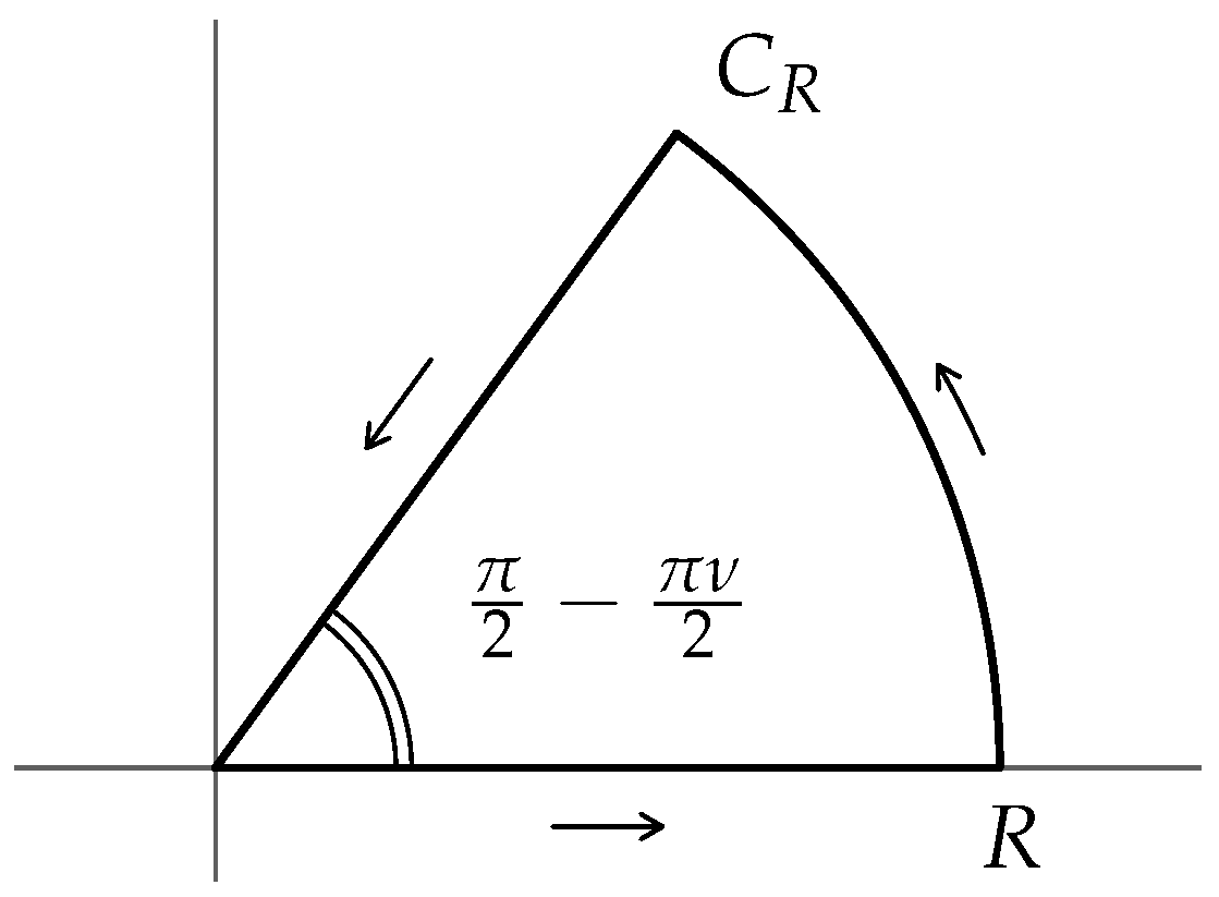
Figure 8.
Path corresponding to the change of variables in the second integral of (44).
Figure 8.
Path corresponding to the change of variables in the second integral of (44).

Figure 9.
Plot of the function f given in (58).
Figure 9.
Plot of the function f given in (58).

Figure 10.
Domain of integration in (60), upon suitable rotation of the axis of the sphere.
Figure 10.
Domain of integration in (60), upon suitable rotation of the axis of the sphere.

© 2020 by the authors. Licensee MDPI, Basel, Switzerland. This article is an open access article distributed under the terms and conditions of the Creative Commons Attribution (CC BY) license (http://creativecommons.org/licenses/by/4.0/).
Share and Cite
MDPI and ACS Style
Iafrate, F.; Orsingher, E. On the Fractional Wave Equation. Mathematics 2020, 8, 874. https://doi.org/10.3390/math8060874
AMA Style
Iafrate F, Orsingher E. On the Fractional Wave Equation. Mathematics. 2020; 8(6):874. https://doi.org/10.3390/math8060874
Chicago/Turabian StyleIafrate, Francesco, and Enzo Orsingher. 2020. "On the Fractional Wave Equation" Mathematics 8, no. 6: 874. https://doi.org/10.3390/math8060874
Note that from the first issue of 2016, this journal uses article numbers instead of page numbers. See further details here.