Article

Algorithmic Analysis of Vesselness and Blobness for Detecting Retinopathies Based on Fractional Gaussian Filters

by
Maria de Jesus Estudillo-Ayala
1,
Hugo Aguirre-Ramos
2,
Juan Gabriel Avina-Cervantes
2,*,†,
Jorge Mario Cruz-Duarte
3,
Ivan Cruz-Aceves
4 and
Jose Ruiz-Pinales
2
1
School of Biological Systems and Technological Innovation, Benito Juárez Autonomous University of Oaxaca, Oaxaca 68020, Mexico
2
Telematics (CA), Engineering Division (DICIS), Campus Irapuato-Salamanca, University of Guanajuato, Carretera Salamanca-Valle de Santiago km 3.5 + 1.8km, Comunidad de Palo Blanco, Salamanca 36885, Mexico
3
Escuela de Ingeniería y Ciencias, Tecnológico de Monterrey, Av. Eugenio Garza Sada 2501 Sur, Col. Tecnológico, Monterrey 64849, Nuevo León, Mexico
4
CONACYT Research-Fellow, Center for Research in Mathematics (CIMAT), A.C., Jalisco S/N, Col. Valenciana, Guanajuato 36000, Mexico
*
Author to whom correspondence should be addressed.
Author thanks the Universidad de Guanajuato by the financial support of the APC.
Mathematics 2020, 8(5), 744; https://doi.org/10.3390/math8050744
Submission received: 20 April 2020 / Revised: 4 May 2020 / Accepted: 5 May 2020 / Published: 8 May 2020
(This article belongs to the Special Issue Mathematical Biology: Modeling, Analysis, and Simulations)

Abstract

:
All around the world, partial or total blindness has become a direct consequence of diabetes and hypertension. Visual disorders related to these diseases require automatic and specialized methods to detect early malformations, artifacts, or irregular structures for helping specialists in the diagnosis. This study presents an innovative methodology for detecting and evaluating retinopathies, particularly microaneurysm and hemorrhages. The method is based on a multidirectional Fractional-Order Gaussian Filters tuned by the Differential Evolution algorithm. The contrast of the microaneurysms and hemorrhages, regarding the background, is improved substantially. After that, these structures are extracted using the Kittler thresholding method under additional considerations. Then, candidate lesions are detected by removing the blood vessels and fovea pixels in the resulting image. Finally, candidate lesions are classified according to its size, shape, and intensity properties via Support Vector Machines with a radial basis function kernel. The proposed method is evaluated by using the publicly available database MESSIDOR for detecting microaneurysms. The numerical results are summarized by the averaged binary metrics of accuracy, sensitivity, and specificity giving the performance values of 0.9995, 0.7820 and 0.9998, respectively.

1. Introduction

The stress, inappropriate feeding behaviors, lack of interest in prevention methods, besides the extensive periods without proper medical screening, have increased the spread of retinal maladies in the world. About 126 million people suffered a kind of Diabetic Retinopathy (DR) in 2011. Such a number could increase up to 191 million by the end of 2030, with around 56.3 million people suffering a vision-threatening complication [1,2]. Regular medical screenings on vulnerable patients (e.g., persons suffering from diabetes or hypertension) may detect ocular problems to prevent permanent blindness in up to 98% of the cases. Although these programs have resulted in a declining prevalence and incidence of DR cases in the United States, European countries, and Australia, in other countries, the DR remains a public health problem. Particularly, some researchers estimated 71% of DR incidence in diabetic patients in Mexico [3,4]. Hence, the increased number of patients brings opportunities for automatic methodologies to help medical experts in accurate disease diagnosis. To determine the degree of DR, medical specialists can use diagnosis techniques based on the analysis of length, orientation, position, and width of the structural elements in the patients’ retina. These detection systems quickly analyze more volumes of information than technicians or specialists. In this way, the functional analysis of retina malformations is crucial to measure and diagnose retinopathy degrees. Such malformations can be, for instance, the exudates, neovascularizations, hemorrhages, and microaneurysms. Most retinopathies are originated by alterations in the blood flow irrigation of the retinal vascular system; such affections can be classified in diabetic, hypertension, and pigmentary retinopathies [5]. Therefore, detection techniques such as segmentation, filtering, and automatic classification should be supported by specialized acquisition systems and technicians. The mechanism for obtaining retinal images, well-known as Retinography, plays a fundamental role in providing high quality and contrast images for many applications, e.g., ocular scan identification in biometrics processes and retinopathies detection in ophthalmology [6]. Besides, some authors took advantage of the retinography diagnostic test to study hypertensive patients [7]. Others showed the reliability of the digital retinography for diabetic retinopathy screening [8]. Hence, computer vision and machine learning applications have focused on contributing meaningfully to the process of diagnosing retinopathies by exploiting these images. For instance, Mansoor et al. proposed a fuzzy methodology to improve the exudates’ contrast for the diabetic retinopathy diagnosis [9]. Narasimhan et al. developed an effective method based on the Arteriovenous Ratio (AVR) for identifying the degree of hypertensive retinopathies [10]. In that work, the blood vessels were classified and segmented using features derived from statistical moments in venules, veins, or arteries, and AVR was simultaneously estimated. Contrarily, El-Abbadi and Hammod Al-Saadi studied several features (i.e., exudates, hemorrhages, tortuosities, and blood vessel diameter) to diagnose diabetic retinopathy [11]. Otherwise, Mamilla et al. detected microaneurysms and hemorrhages in retinal images by employing an effective combination of phase congruency from Log–Gabor filters and mathematical morphology [12]. After identifying the potential lesions, the authors labeled them using a set of 18 attributes through a supervised classifier such as k-Nearest Neighbors (kNN) or Support Vector Machines (SVM). Similarly, Rahim et al. proposed a system that classifies images depending on the detected microaneurysms [13]. To do so, they employed six features (namely area, perimeter, distance around the boundary of the region, major and minor axis length, aspect ratio, and circularity of the candidate) on four classifiers (binary decision trees, kNN, and two SVMs using a radial basis function and polynomial function kernels). Jiménez et al. proposed a method for searching microaneurysms, implementing a classification rule based on the attributes of a lesion candidate such as the intensity, size, and form, which was obtained through a region growing process [14]. The initial points (seeds) of lesion candidates are collected via the Burg algorithm on an image enhanced by a high-pass filter and a top-hat morphological operator. On the other hand, Walter et al. applied a polynomial contrast-enhancement filter to increase the recognition of the microaneurysms [15]. There, they selected the candidate lesions by a diameter closing and a top-hat transformation, which allowed extracting 15 features based on the size, form, and intensity of the lesions. This classification problem was carried out by Kernel Density Estimation (KDE). Furthermore, Navarro et al. proposed a system combining user-defined thresholding on the enhanced L * and a * channels through an illuminant normalization and a Wiener filter [16]. From this combination, they employed a series of three features, namely, area, eccentricity, and center of mass, to detect the candidate lesions that give the result via texture classification. Such a classification is obtained by applying wavelet transforms to the candidate regions and utilizing a kNN algorithm. However, the authors only considered the image segmentation focused on microaneurysms and hemorrhages for being subsequently used in an automatic diagnostic system. The very low-contrast between these biological structures and the image background, the remarkable variations on size and distinctive shape, besides the proximity to the optic nerve, fovea, or blood vessels make difficult the accurate recognition of the suspicious lesions.
This work aims aims to contribute to the accurate recognition of retinopathies, particularly microaneurysm and hemorrhages. For that purpose, we present an innovative framework powered by a multidirectional filter based on the Fractional-Order Gaussian Function (FOGF). This filter is adjusted via a well-known optimization algorithm, such as Differential Evolution (DE). The application of such a filter meaningfully improves blood vessel contrast, as well as positively enhances the delimiting region of retinal aneurysms. The framework also includes the Kittler thresholding method under additional conditions for extracting the microaneurysms and hemorrhages structures. Thenceforth, candidate lesions are detected by removing the blood vessels and fovea pixels from the resulting image. Finally, these lesions are classified according to their size, shape, and intensity properties via SVM with a radial basis function kernel. The proposed method is evaluated by using the publicly available database MESSIDOR for detecting microaneurysms. Results show astonishing characteristics of this method for identifying microaneurysm structures in most of the studied cases.
The remainder of this document is organized as follows: Section 2 briefly describes the medical concepts related to retinopathy diagnosis. Section 3 presents the proposed methodology, as well as some practical considerations. Subsequently, Section 4 details the methodology carried out and the corresponding experimental results. Finally, Section 5 summarizes the most relevant conclusions.

2. Background

Retinography is a noninvasive diagnostic technique that certainly does not use contrast agents in the acquisition process [17]. This technique produces color images from the inner part of an eye, well-known as Fundus Images (FIs), which can be used to detect some diseases, e.g., diabetic retinopathies and glaucoma. These images are characterized by a quasi-circular shape with a small rectangular flange that represents the Field of View (FoV) of the capture device. Figure 1 shows the typical internal structures composing a fundus image.
In general, the fundus images from healthy-patients have four common elements: the optic disk, blood vessels, fovea, and macula (see Figure 1). The Optic Disk (OD) is a circular and bright structure that interconnects the internal and external parts of the eye. Crossing the OD, there are the blood vessels and optic nerve [8]. The blood vessels are typically reddish tubular structures that exchange oxygen and move essential nutrients from and into the human eye. These structures, identified as veins and arteries, are spread in the image as a complex network connected with smaller elements known as venules and arterioles in their extremities. Found close to the optic disk is the fovea, visually recognized as an oval or circular red region. This element is extensively irrigated by the choroid, which is a membrane free of blood vessels. Located in the fovea, the biological photoreceptor cells, namely cones and rods, transform the light stimuli into electrical signals transmitted by the optic nerve to the brain. Additionally, the fovea is surrounded by the macula that is specialized in the perception of details. Under certain circumstances, specific features of these elements are used to determine the physical or mental health of a patient. For instance, recent studies have shown a direct link between the retinal state and its association and potential use in the diagnosis of dementia [18], Parkinson’s [19], and Alzheimer’s diseases [20], as well as other cognitive deficits [21] and neurodegenerative conditions [22]. In the same context, modifications in shape and optic disk size are a clear pointer to serious illness like glaucoma. However, different circumstances influence the appearance of extraneous biological structures in FI, most of them attributed to retinopathies. Retinopathy is a noninflammatory retina disease that can also include other medical conditions [10,18,20]. Particularly, diabetic and hypertensive retinopathies are the most studied and well-known retinal diseases. Both medical conditions may provoke similar symptoms (i.e., extraneous structures in the image), but the number, shape, size, and apparition probability may distinctively characterize each disease. Besides, its presence in the retina is highly influenced by the disease evolution degree. These representative structures are used as a starting point for the diagnostic assessment of retinopathies. Figure 2 illustrates the most distinctive structures characterizing retinopathies, such as neovascularization, hemorrhages, exudates, and microaneurysms.
Specifically, the neovascularization ( N V ) is related to a new blood vessel generation produced by a prolonged lack of blood in specific regions of the eye [23]. It is usually a consequence of diabetic retinopathy. Nevertheless, due to the stressing process of how these new blood vessels were created, they generally have irregular, weak, and low-quality walls prone to rupture. Plus, these blood vessels may come up as saliencies in the contour of the optic nerve, as shown in Figure 2a. The retinal hemorrhages (H) typically appear when blood vessel membranes get weak and start to bleed. But it is also provoked by changes in blood composition or disturbances in circulation [24]. Hence, blood is accumulated in the retina or vitreous humor. These hemorrhages produce irregular reddish spots in the fundus image, like those observed in Figure 2b. In critical cases, hemorrhages may produce partial or complete blindness because photoreceptor cells suffer from light occlusion and are barely stimulated. Moreover, the exudates (E) are typically generated when proteinic substances are spread into the eye from blood vessels, forming brilliant depots varying their size from small spots until large zones in the FI. Some exudates surrounding the fovea are displayed in Figure 2c. Like N V , this pathology is also caused by diabetic retinopathy. The last characteristic structure of retinopathy is the microaneurysm ( m A ), which appears as small reddish spots in different zones of the FI (see Figure 2d). These could be easily confused with small punctual hemorrhages. However, the m A is induced by the blood vessel dilations but not by draining blood out to the vitreous body. This specific set of undesired structures is used for diagnosing both the Retinopathy Degree (RD) and Macular Edema Risk (MER). Furthermore, Table 1 contains the respective constraints for the diagnostic evaluation of RD and MER, considering the occurrence frequency of microaneurysms, hemorrhages, and neovascularization.
Under the diagnosing parameters, a patient is considered free of any retinopathy when R D = 0 , while a patient suffering the worst symptoms of such disease may get R D = 3 . Moreover, MER is evaluated considering the occurrence of exudates; when they are detected, there is a substantial risk of macular edema if the MaCula to Exudate distance is inferior to the optic disk diameter, M C E ^ min D OD [26]. Consequently, the number of m A and H can be used, almost independently, as an efficient estimator of retinopathies. Such a premise is the central axis of this study.

3. Materials and Methods

The proposed framework uses images from the public database MESSIDOR [25]. This database comprises 1200 images aimed to develop methods for diagnosing diabetic retinopathies. Each image has the RD and MER diagnosis provided by experts according to the disease evolution. For evaluation and learning purposes, this work employs the m A delineations generated by Habib et al. in [27,28]. The flowchart depicted in Figure 3 presents the main blocks of the proposed method.
At first, the input color image is decomposed into the corresponding RGB channels. The green channel is selected because it presents the highest contrast, instead of computing the traditional gray level images by averaging the three RGB channels. This choice is computationally more efficient, and according to color theory, the green channel contains more details and less noise than other channels. In the upper-branch of the processing flow, the Fractional Order Gaussian Filters (FOGF) and Kittler thresholding method are applied to the selected image channel. The FOGF filters are proposed to ease the task of detecting the small H and m A structures. These operate mainly as feature descriptors and functionally enhance the detection of the structures by improving the contrast. Thus, the filter parameters are tuned by using a metaheuristic optimization method. The Differential Evolution (DE) algorithm was chosen due to its efficiency and relative simplicity of implementation. Hence, the FOGF filters are focused on detecting H and m A . Moreover, given their fractional-order nature, they are applied in eight preferential orientations. Next, a thresholding process based on spatial constraints over the Kittler minimal error method is applied to the filtered image, which extracts several complex structures from the background. In the lower-branch of the process, an algorithm for identifying both blood vessels [29] and fovea based on an efficient conics detection method [30] was implemented. A differential outcome is obtained by subtracting the partial results from both branches (see Figure 3) to discriminate the structures of interest. At this stage, some pixels belonging to other structures such as the fovea or blood vessels are found. These are eliminated by identifying the pixels related to a specific structure and then removing them from the binarized image. As a result, a set of candidate lesions is found. Afterward, a series of five features are extracted from each candidate lesion, i.e., the size, eccentricity, mean, and minimum intensity of the FOGF filter response, and length of the major axis of the ellipse that contains the candidate lesion. Finally, from these features, m A and H lesions are found by applying an SVM classifier over this collection of features.

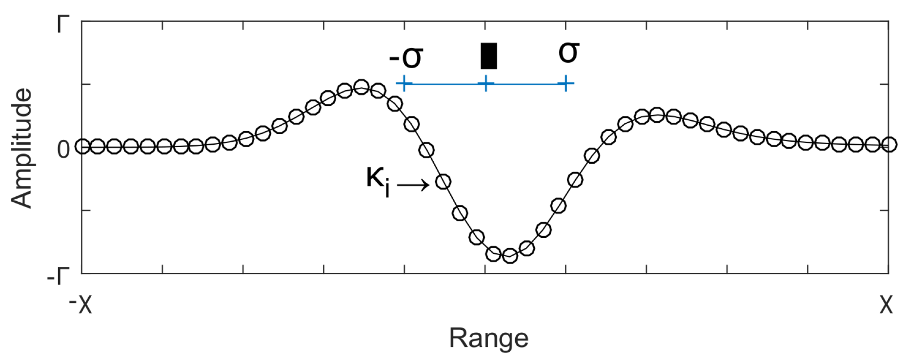
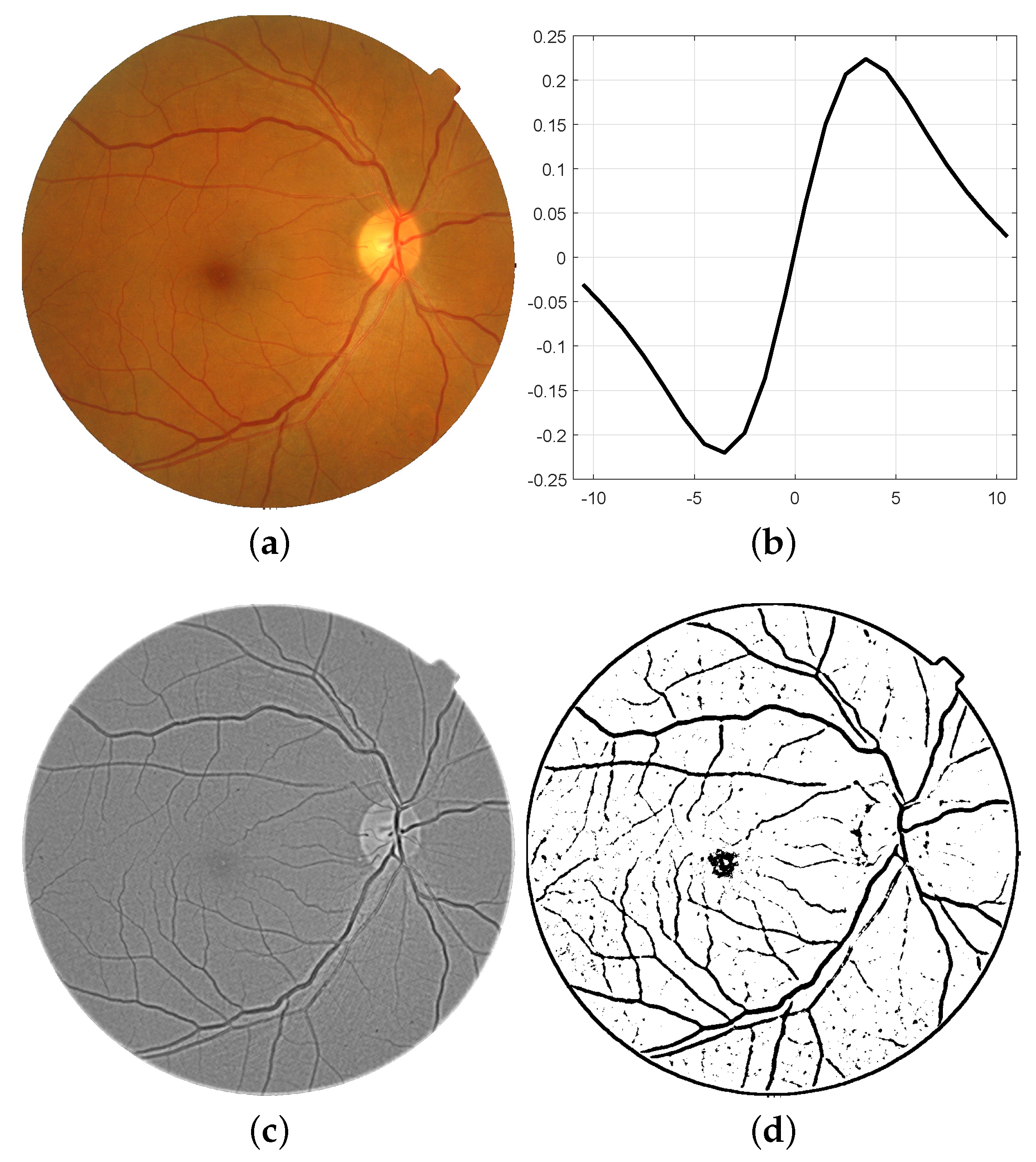
3.1. Fractional Order Gaussian Filters

Since the successful application in anomalous diffusion [31], the fractional calculus has found a vast number of uses on pattern recognition, image denoising [32,33], and texture enhancement [34].
In the literature, there exists a variety of definitions for the fractional differential operator, such as Liouville, Riemann–Liouville [35], Caputo, Caputo–Fabrizio [36], Grünwald–Letnikov [37], Weyl, Marchaud [38], Hadamard [39], Chen [40], Chen–Marchaud [41], Fourier transform [42], among others [43]. In practice, this operator is selected according to its properties and suitability to the problem to analyze. So, we implemented the operator presented by Tseng et al. [44], which is defined as follows
D x ν f ( x ) = 1 2 π ( i ω ) ν F ( ω ) exp i ω d ω ,
where ν [ 0 , 2 ] , D x ν f ( x ) represents the ν -order fractional derivative of the function f ( x ) , and F ( ω ) = F { f ( x ) } ( ω ) is the Fourier Transform of the same signal. This definition is used to generate the FOGF filter bank.
Thus, four filters are shown in Figure 4 by using the Gaussian function N x ( μ , σ ) as the base function f ( x ) ,
f ( x ) = N x ( μ , σ ) = 1 2 π σ exp ( x μ ) 2 2 σ 2 ,
since μ is the mean and σ 2 is the data variance. Using Fractional-Order Gaussian Filters as a texture descriptor is pretty recent in image processing. Moreover, these are turning out especially suitable for texture applications when fractional orders ν 1 are employed. In fact, a recent study of the fractional calculus applied in image processing was extensively discussed in [45]. Such work presented the discretization of most used fractional-order derivatives validating their advantages on improving image analysis. Hu et al. proposed a fractional differential operator mask with a non-integral adaptive step and fractional order to enhance the texture and analyze its features [34]. In practice, it is noticeable that FOGF presents similar behavior as the Difference of Gaussians (DoG) filters, which may extend the number of applications.

3.1.1. Model Parameters Selection

All the FOGFs are generated using the kernel D x ν N x ( μ , σ ) obtained with (1) and the normal distribution function N x ( μ , σ ) . In such a kernel, a set of four parameters should be estimated, i.e., the fractional-order ν , the domain x, the mean μ , and the standard deviation σ . However, to determine x two parameters (n and χ ) are required, such that x is rendered by n elements K i uniformly distributed in the interval [ χ , χ ] . Figure 5 shows an illustrative example of the kernel parameters.
It is noteworthy that asymmetry is detected on this profile, which is produced by the fractional nature of the filter. Withal, the vector of kernel parameters is represented by X = ( ν , χ , n , μ f , σ f ) having six design elements, i.e., X R 6 . Determining the optimal values of these six parameters requires an exhaustive evaluation that is generally time-demanding and impractical. In particular, if each parameter is tuned at a time. Naturally, to obtain the reliable and optimal performance of the proposed filters, it is fundamental to simultaneously determine all the parameters and anticipating a certain degree of dependency between them. Therefore, the vector X is estimated by using the Differential Evolution (DE) algorithm.

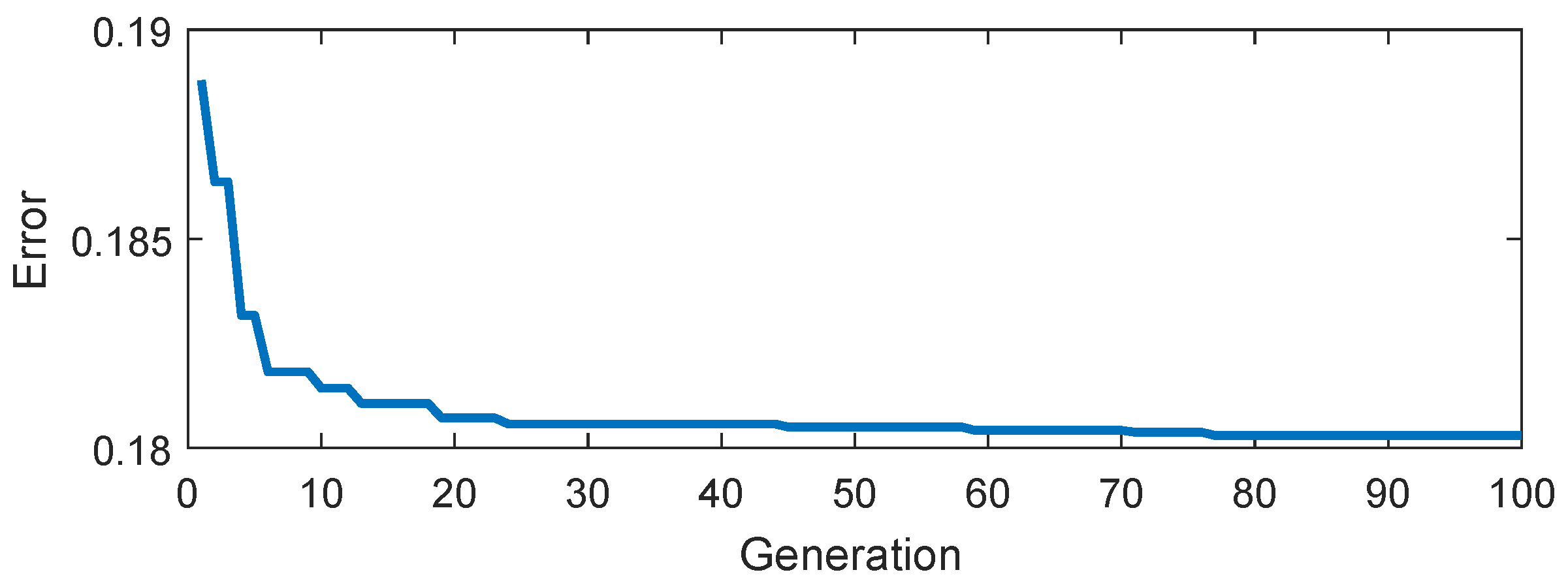
3.1.2. Differential Evolution (DE) Algorithm

DE is a well-known optimization method characterized by its relative tuning simplicity and effectiveness for solving multiparametric problems. This algorithm was proposed by Storn and Price [46] as a method based on an evolutive mechanism. DE starts generating an initial population at random, and finds the optimal solution by fitting the experimental data to a given model representing the problem. This technique uses some strategies to combine the initial population for the posterior choice of the best individuals per iteration. After each combination, a mutation function is applied to generate new diversified individuals. The canonical implementation of this algorithm comprises four stages: initialization, mutation, crossover, and selection. Hence, there are N candidates in the population P, each candidate has a position (solution) vector given by X R D , which are initially estimated via the uniform distribution into the search space. During each generation (iteration) G, every individual in the population is considered as an objective vector X i G . In the mutation stage, at least two donor elements X r i G , randomly chosen with r i U I ( 1 , N ) and i { r i } = , are combined to create the new donor solution vector u I G + 1 that may interact with the next generation G + 1 . In this work, the combination strategy is defined by
u i G + 1 = X r 1 G + F 1 ( X r 2 G X r 3 G ) + F 2 ( X b e s t G X i G ) ,
where F 1 and F 2 are the mutation factors, and X b e s t G is the objective vector corresponding to the best model adjustment in the current generation. Experimental experiences allowed choosing the values for these factors such as F 1 = 0.5 and F 2 = 0.01 . For the crossover stage, some internal components of the donor vectors are randomly modified by using a threshold C R [ 0.0 , 1.0 ] . The crossover function produces a test vector v i G that diversifies the population at each iteration. The components of v i G are obtained as shown
v i j G + 1 = u i j G , if r u C R j = I u X i j G , if r u C R j I u ,
where v i j G v i G , u i j G u i G , X i j G X i G , Z + + i N , and Z + + j D . r u U ( 0 , 1 ) is a random number generated from the standard uniform distribution, and I u U I ( 1 , D ) is an integer randomly selected from the interval [ 1 , D ] . Moreover, the threshold value C R = 0.5 was determined from an exhaustive experimentation process. Finally, during the selection phase, the best individuals satisfying the model are chosen among the test v i G and objective vectors X i G . The last three stages of the DE algorithm are successively repeated until the convergence criterion is satisfied.

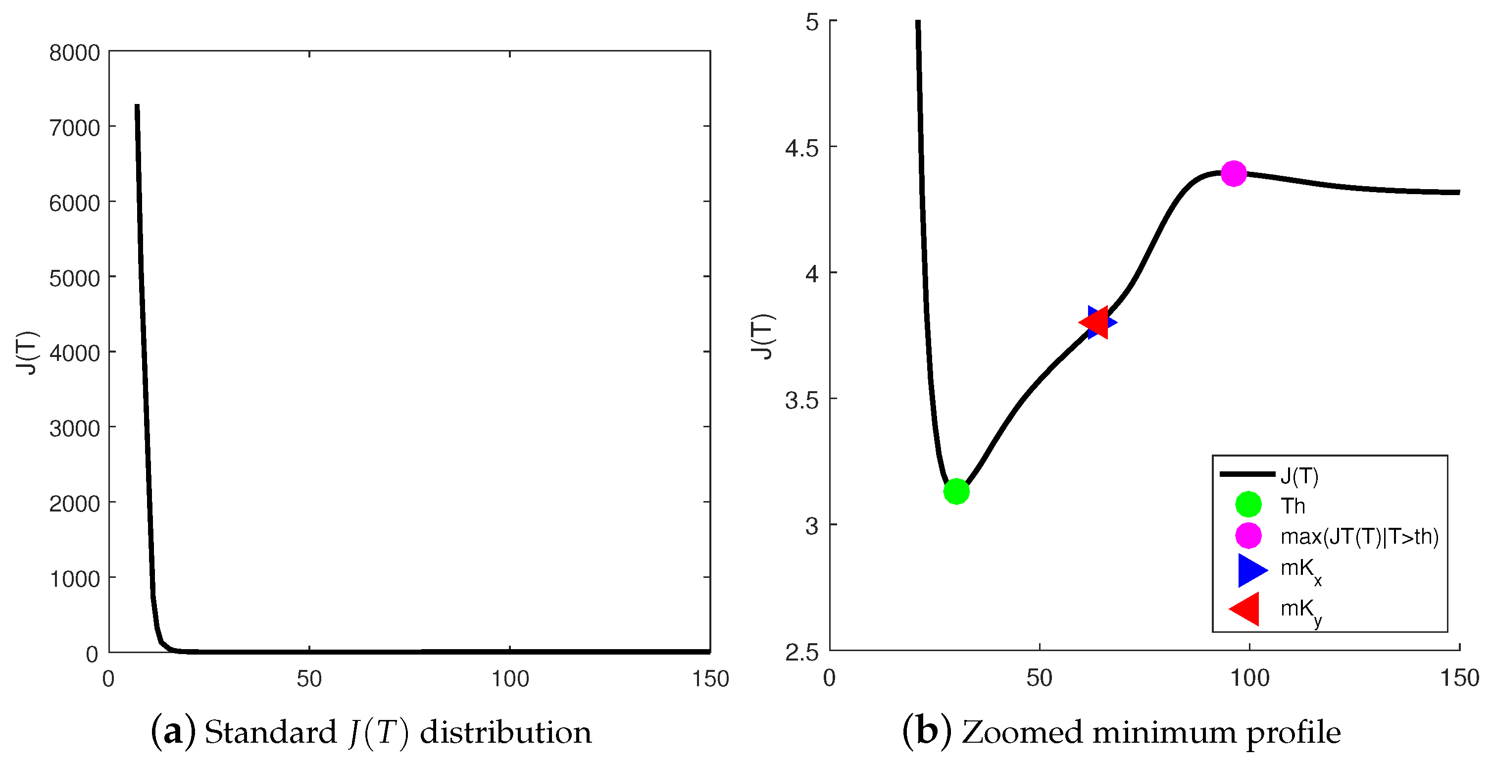
3.1.3. Objective Function

The performance of the response image I m R is analyzed to select the candidate vectors containing the optimal parameters. This image is obtained by adding all the responses of the retinal image I m convolved with the FOGFs bank D x ν N x ( μ , σ ) . Given that fractional filters are intrinsically asymmetric, they were applied on eight directional configurations, i.e., θ k = 2 π k / 8 , k { 0 , 1 , , 7 } to avoid preferential directions (spatial bias). These configurations can be visually represented by { , ↗, ↑, ↖, ←, ↙, ↓, } . Such a generalization to 2D fractional filters was previously studied by Chen et al. in the context of image-enhancing [47]. Therefore, I m R is determined through
I m R = k = 0 d 1 I m D x ν N x k ( μ , σ ) ,
where ∗ is the convolution operator, and D x ν N x k ( μ , σ ) corresponds to the k-th FOGF using the parameters X i G oriented with the directional configuration k. Furthermore, it is required to define an objective function to evaluate the performance of the FOGF for a given candidate vector X i G during the DE process. Such a function is stated as
f o b j ( α , β ) = arg min i 1 α β X i ( T ) Y i ( T ) d T ,
where X i and Y i are the True Positive Rate and the derivative of the False Positive Rate for a candidate X i G , respectively. These metrics are computed simultaneously on the response image I m R and the reference binary image I m B [ 0 , 1 ] in the threshold interval T [ α , β ] . The aforementioned metrics are defined by
X ( T ) = | ( I m R < T ) I m B | | I m B | ,
Y ( T ) = | ( I m R < T ) ( 1 I m B ) | | 1 I m B | ,
since | · | is the cardinality operator.

3.2. Kittler Thresholding Method

This histogram-based thresholding method was proposed by Kittler and Illingworth [48]. It searches a minimal probabilistic decision error in a supposing bimodal distribution. They considered that a gray level image with g = 2 n pixel values can be separated into two planes, background and foreground, by using the image histogram h ( g ) . So, h ( g ) represents both planes by the addition of at least two probability distributions p i ( g ) . These functions are modeled as normal distributions using only the means μ i and variances σ i 2 . Besides, by employing the a priori probability P i i { 1 , 2 } , the complete distribution becomes
p ( g ) = i { 1 , 2 } P i 1 2 π σ i exp ( g μ i ) 2 2 σ i 2
According to the Bayes theorem, the optimal threshold T h separating both distributions yields the minimal decision error. This threshold can be found by using the following reduced function
J ( T ) = 1 + 2 [ P 1 ( T ) log σ 1 ( T ) + P 2 ( T ) log σ 2 ( T ) ] 2 [ P 1 ( T ) log P 1 ( T ) + P 2 ( T ) log P 2 ( T ) ] ,
where P i ( T ) = g = a b h ( g ) , μ i ( T ) = g = a b g h ( g ) / P i ( T ) , and σ i 2 ( T ) = g = a b ( g μ i ( T ) ) 2 h ( g ) / P i ( T ) for the interval [ a , b ] established as [ 0 , T ] for i = 1 and [ T + 1 , n ] for i = 2 . Therefore, the minimal error threshold T h is estimated such as
T h = arg min T { J ( T ) } .
However, for images having a high density of low-intensity pixels, the obtained threshold could be useless as they are polarized to dark gray levels. Notice that the error function proposed by Kittler presents a high probability of finding points with a low-intensity when J ( T | T 0 ) J ( T | T ) . Consequently, reliable thresholds are found to some extent far from the low bins in the histogram. Extensive experimentation allowed to accomplish such condition by finding the inflection point between the interval [ T h , max ( J ( T | T > T h ) ) ] , which is depicted in Figure 6.
This rule is applied even if this point was computed as the point T i such as J ( T i ) 0 and verified a sign change in J ( T i ) . In this work, for the sake of the numerical stability, the threshold is approximated to the averaged point T m k in the interval T [ T h , max ( J ( T | T > T h ) ] as given
T m k arg min T J ( T ) max J ( T ) min J ( T ) 2 s . t . T > T h

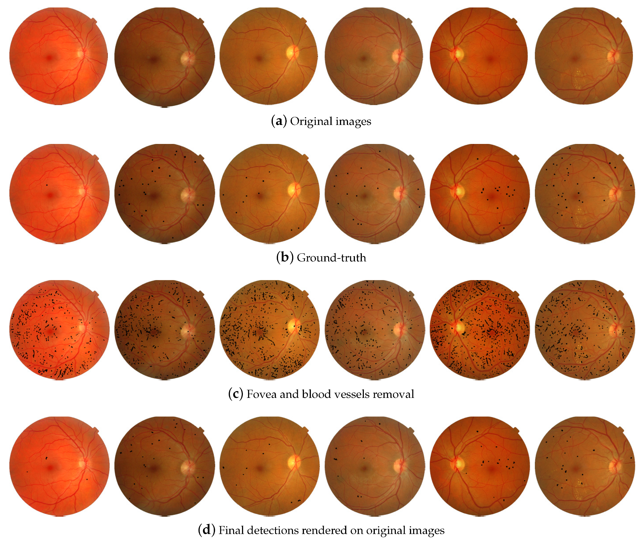
3.3. Blood Vessels and Fovea Correction

Blood vessel extraction and fovea detection are not the central subjects of this study, but considering their intensity features, they could appear next to aneurysms and hemorrhages after thresholding. Therefore, these structures should be identified and removed previous an extensive image analysis. In such a sense, some methodologies are then proposed for this detection.

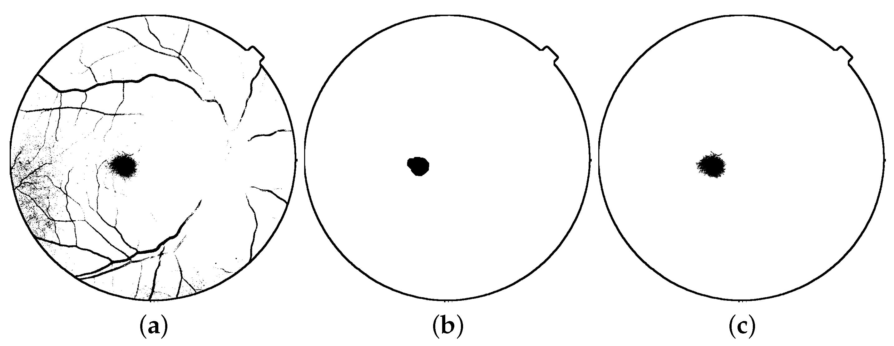
3.3.1. Fovea Detection

Concerning the ellipsoidal (or circular) shape of the fovea, this structure may be correctly identified by applying a conic detector filter on the retinal image I m R . However, some lesions may appear close to the fovea leading to inaccurate results and misdetection of microaneurysms and hemorrhages. Thence, an intensity-based segmentation that preserves the fovea irregularities is used. In that context, the estimated threshold image f t h is obtained by binarizing the green channel of I m R via the Kittler thresholding method. Next, the undesired tubular and punctual structures are removed by using the morphological operator having a circular shape and radius 12 ( D 12 S ) structural element. The foveal image is then computed by
I m f = f t h D 12 S .
It is essential to notice that given the problem nature, it may be necessary to use a complete version of the fovea, instead of the one given by the image opening. This element can be obtained via the region growing given by I m f as the seed over image f t h . Figure 7 depicts an example of the proposed methodology to extract the fovea region.

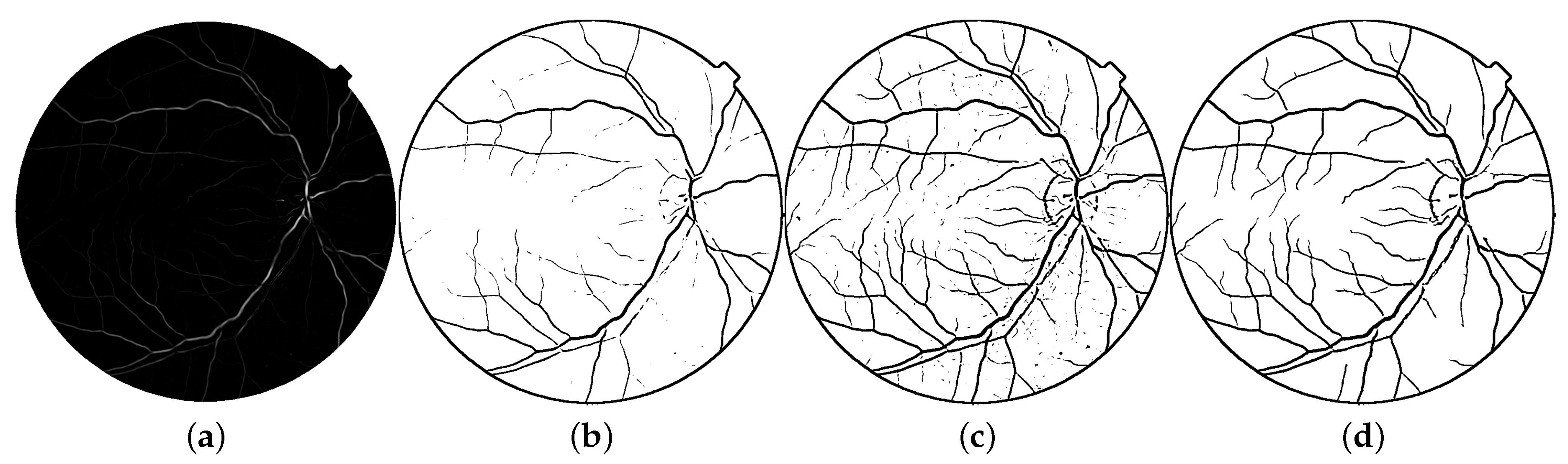
3.3.2. Blood Vessels Detection

Blood vessel extraction uses the Frangi method [49]. This method employs a specialized filter to enhance tubular structures, which is based on calculating the eigenvalues λ i of the Hessian matrix
H = 2 x 2 2 x y 2 x y 2 y 2 I m r .
Nonetheless, to control the width in the tubular structures, the direct partial derivatives are substituted by the smoothed partial derivatives of a Gaussian filter N X Y = 1 2 π σ exp x 2 + y 2 2 σ 2 with mean μ = 0 and variance σ 2 , such as
H N X Y = 2 x 2 N X Y 2 x y N X Y 2 x y N X Y 2 y 2 N X Y I m r .
Thus, the vascularity function V o in (16) is determined by the eigenvalues of H N X Y , where the variables α , β , and γ represent the thresholds controlling the filter sensibility.
V o = 0 , if λ 2 > 0 λ 3 > 0 , 1 exp λ 1 2 2 α 2 λ 2 2 1 exp k = 1 3 λ k 2 2 γ 2 exp λ 1 2 2 γ 2 | λ 2 λ 3 | , otherwise .
Different diameter structures are detected using a variety of scales in the Gaussian filter. Hence, the result is obtained by computing the maximum value of the vascularization function sweeping over different scales. Considering a certain number N of scales in a searching range σ [ σ m i n , σ m a x ] , the vascularity image is calculated by
H l = arg max σ m i n σ σ m a x V o ( σ ) .
For this study, the particular parameters for the vessel detection are σ [ 2 , 3 ] and N = 21 (i.e., steps of 0.05), and ( α , β , γ ) = ( 1.0 , 2.25 , 15 ) . Due to the nature of this image (vasculature with both high and low intensities), the conditions for the application of modified Kittler thresholding are not achieved. Therefore, the original Kittler algorithm should be used. Nevertheless, the original Kittler method also fails to find the complete vascularity network. This negative effect is seen in Figure 8b, where only the major vasculature is completely detected.
Given that the main objective of this work is the removal of blood vessels in the original image rather than a precise detection, a length filter with a fixed threshold is exploited. This last threshold is applied to the normalized version of the vascularity image ( V l ¯ = V l [ 0 , 255 ] ). Under these circumstances, a threshold value of t h c = 0.01 is used to create the candidate V s c image by V s c = V l ¯ > t h c . Finally, the vascularity image is segmented utilizing the length filter given as
V ( n ) = 1 , if | V s c ( n ) | > t h a 0 , otherwise , n = { 1 , 2 , , N } ,
where t h a corresponds to the minimal area that is maintained by the n-th region in V s c = n V s c ( n ) to be considered as a blood vessel. A representative result using the fixed length filter ( t h a = 100 ) is also presented in Figure 8d.

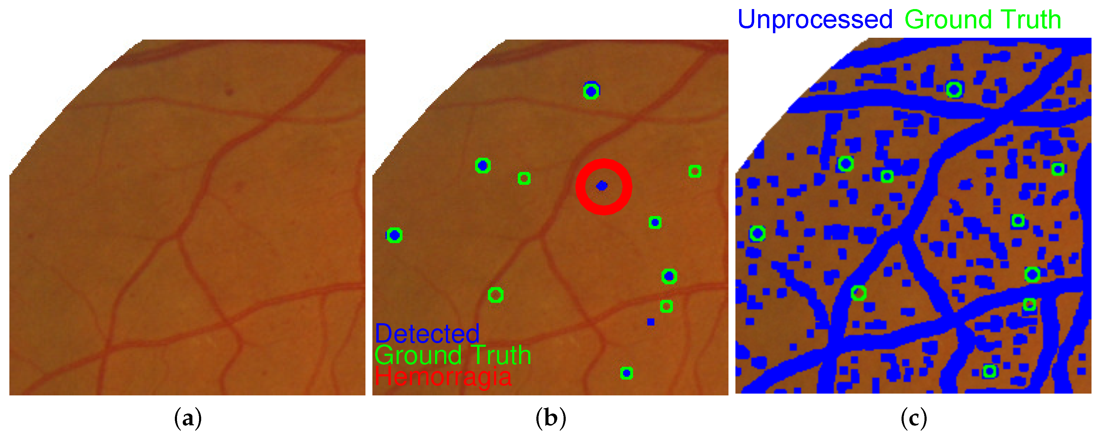
3.4. Candidate Lesion Classification

Even though the removal of fovea and blood vessel pixels could produce a set of candidate lesions, such collection could still include undesired elements such as unconnected vessels, spurious lesions, or speckle noise. All candidate lesions are passed through an SVM classifier to decide whether a candidate could represent a microaneurysm ( m A ) or hemorrhage (H). It uses an optimization method to identify support vectors s i , weights w i , and bias b i , which are employed to classify vectors x into a class c according to
c = i a i k ( s i , x ) + b i ,
where k is the kernel function. For this study a radial basis function kernel, k ( s i , x ) = exp s i x 2 , was used. The candidate lesions represented by a vector x is composed of five features: size, eccentricity, the average and minimum intensity of the FOGF response, and length of the major axis of the ellipse containing the candidate lesion. Each feature is selected to cope with the specific properties of undesired candidates.

4. Numerical Results

All experiments in this study were carried out in a PC with Intel®Core™i5-6200U CPU @ 2.3–2.4 GHz, and 8 GB RAM. The algorithms were coded and evaluated in MATLAB®R2016a running on Microsoft®Windows™10 OS. The design of optimal filters for improving contrast as well as enhancing features are complex tasks, but fundamental in medical imaging. Such a complexity relies on a high number of parameters for tuning and a close correlation among them. The adverse effects of this correlation are reduced by simultaneously adjusting all filter parameters. For this purpose, the DE optimization algorithm was implemented, and its parameters C R , F 1 , and F 2 were analyzed by combining exhaustively of their values. The chosen values that provide the best results were C R = 0.5 , F 1 = 0.5 , and F 2 = 0.01 . Figure 9 depicts the objective function value (error) evolution during the tuning process.
Bear in mind that the evolution of f o b j (cf. (6)) is plotted for 100 generations. An averaged error of 0.1888 is found only in the first generation. However, the DE method evolves towards a better solution with each new iteration. Therefore, the model coefficients can be selected from a wide range of combinations (or search space) without significant variation in errors. In the implemented version, the parameters were constrained to positive values and rounded to the upper integer. DE allowed determining the best performance by tuning the FOGF, as Figure 10b shows.
Subsequently, Figure 10c presents the resulting image after applying these filters to a retinal image. Still, FOGFs detect not only microaneurysms but also blood vessels, fovea, and hemorrhages. Such undesired misclassifications can be attributed to the objective function properties and the intensity similarities between the target structures. Contrarily to the resulting image presented in Figure 10b, the exudates are distinguished and extracted from the one shown in Figure 10d. This last result was computed using the Kittler thresholding, where microaneurysms, hemorrhages, blood vessels, and some fovea pixels are accurately detected. It is noteworthy that the method selectivity on detecting microaneurysms and hemorrhages is boosted by using peculiar features, shapes, and sizes. Figure 11 exhibits microaneurysms and fovea detection. Previously, the fovea and blood vessels removal function was efficiently executed.
Notwithstanding, a severe retinopathy ( G R = 3 ) was correctly diagnosed in this image. The redundancy of information and the sufficient number of the structural elements allowed obtaining this complicated diagnosing. So, four binary metrics, accuracy (Acc), balanced accuracy (BAcc), sensitivity (Sen), and specificity (Spe) were selected for evaluating the classification of proposed method [50]. These measurements are determined from a binary image A and a reference image B (ground-truth) as follows
A c c = T P + T N P + N = | A B | + | A ¯ B ¯ | | B | + | B ¯ | ,
B A c c = T P P + T N N = | A B | | B | + | A ¯ B ¯ | | B ¯ | ,
S e n = T P T P + F N = | A B | | A B | + | A ¯ B | ,
S p e = T N T N + F P = | A ¯ B ¯ | | A ¯ B ¯ | + | A B ¯ | ,
where T P stands for True Positives, i.e., points designated as positive in binary image A that also appear as positives in reference image B (or simply A B ); T N corresponds to True Negatives, i.e., points in A marked as negative that also appear as negatives in B (or A ¯ B ¯ ); F N means False Negatives, i.e., points established as negatives in A but which appear as positives in reference image B (or A ¯ B ); F P defines the False Positives, i.e., points labeled as positives in A that are designated as negatives in B (or A B ¯ ). B and B ¯ symbolizes the Positive and Negative counted values of B respectively, and | · | represents the cardinality operator. These metrics produce a continuous output in the interval [ 0.0 , 1.0 ] since 1.0 indicates the perfect matching between the images A and B. The evaluation of microaneurysms detection is summarized in Table 2.
There, an average balanced accuracy of 0.8909 and an average sensitivity of 0.7820 were singularly representatives. Note that all detected regions were considered to build this table. Accordingly, the results contain only a few pixels belonging to hemorrhages or blood vessels. Thus the size could allow discriminating between microaneurysms and hemorrhages, the retinopathy degree is assigned by computing the number of detected elements from each one of the classes. Results of microaneurysms and hemorrhages detection are shown in Figure 12. The proposed method gives the results depicted in Figure 12b, and the result after applying the Kittler thresholding method is presented in Figure 12c. In that image, the reference microaneurysms are displayed in green and those detected by the proposed method in blue. As expected, the result obtained by applying the thresholding method contains the majority of microaneurysms. Nevertheless, the proximity of these structures with some blood vessels gave rise to their elimination from the final result. In consequence, an efficient and robust method to detect and remove blood vessels is highly necessary for improving results. Moreover, most dispersed points in the reference image belong also to pixels from blood vessels, but they correspond to narrower blood vessels than the regular, continuous structures.

5. Conclusions

In this paper, an innovative framework for enhancing and detecting microaneurysms in fundus images is presented. It applies a multidirectional filter based on Fractional-Order Gaussian Filters (FOGFs). On the one hand, the internal parameters of this filter were simultaneously adjusted by using the well-known Differential Evolution (DE) algorithm. On the other hand, a modification to the Kittler thresholding method to cope with histograms containing a high density of low-intensity points was also implemented. The proposed method was evaluated on the publicly available database MESSIDOR for detecting microaneurysms. This methodology provided acceptable results for enhancing and detecting microaneurysms, which an average accuracy of 0.9995 and an average sensitivity of 0.7820 for the global detection process. Moreover, the method was able to enhance and detect hemorrhages that were separated from microaneurysms using shape and size features. Microaneurysms rendered irregular shapes, contrarily to hemorrhages that are characterized by punctual or quasi-circular shapes. Under these circumstances, the obtained results can be utilized to classify the degree of retinopathy present in patients by employing as support the parameters given in Table 1. The number of detected structures is highly relevant for microaneurysms and hemorrhages diagnosing. Thus, when a single microaneurysm point is detected, this should be included in the general account directly affecting the diagnosis. Finally, the proposed method is extremely competitive for detecting at least one microaneurysm structure in most studied cases. Finally, the proposed approach can found some potential applications for detecting similar patterns in medical imaging. For instance, on digital mammograms, the effective localization of microcalcifications is highly demanded, in such a problem, the early detection of tiny abnormal structures in the woman’s breasts is a priority. Moreover, the microcalcifications are also commonly found in affections derived from medical disorders in the brain, liver, and thyroid gland, which justify a broader prospective evaluation of the proposed method.

Author Contributions

Conceptualization, M.d.J.E.-A. and H.A.-R.; Methodology, J.G.A.-C. and H.A.-R.; Software, H.A.-R. and J.G.A.-C.; Validation, J.M.C.-D., I.C.-A. and J.R.-P.; Formal analysis, J.G.A.-C., I.C.-A. and H.A.-R.; Investigation, M.d.J.E.-A., H.A.-R. and J.G.A.-C.; Data curation, J.M.C.-D., I.C.-A. and J.R.-P.; Visualization, M.d.J.E.-A., I.C.-A. and J.M.C.-D.; Writing—original draft preparation, H.A.-R., and M.d.J.E.-A.; Writing—review and editing, J.G.A.-C. and J.M.C.-D. and J.R.-P.; Funding acquisition, J.G.A.-C. and J.R.-P. All authors have read and agreed to the published version of the manuscript.

Funding

The APC was funded by the Universidad de Guanajuato.

Acknowledgments

This project was fully supported by the Electronics Engineering Department of the Universidad de Guanajuato under the Program POA 2020, grant NUA 143079, and the Mexican Council of Science and Technology CONACyT, grant number 398704/473661.

Conflicts of Interest

The funders had no role in the design of the study; in the collection, analyses, or interpretation of data; in the writing of the manuscript, or in the decision to publish the results.

Abbreviations

The following abbreviations and symbols are used in this manuscript:
DEDifferential Evolution
SVMSupport Vector Machines
MESSIDORMethods for Evaluating Segmentation and Indexing Techniques Dedicated to
Retinal Ophthalmology
DRDiabetic Retinopathy
AVRArteriovenous Ratio
kNNk-Nearest Neighbors
KDEKernel Density Estimation
CIE-LABCommission Internationale d’Éclairage L * a * b *
FOGFFractional Order Gaussian Filter
FIFundus Images
ODOptic Disk
FOVField of View
N V NeoVascularization
Hretinal Hemorrhages
m A MicroAneurysm
MERMacula Edema Risk
RDRetinopathy Degree
M C E MaCula to Exudate distance
DoGDifference of Gaussian filters
N x ( μ , σ ) Normal Gaussian Distribution
D x ν f ( x ) ν -th Fractional Derivative of f ( x )
Z + + Positive Integers and zero
arg min x f A point x in the domain of f ( x ) where the function is minimized
f s Opening of f ( x ) by a structuring element s
f s Dilation of f ( x ) by a structuring element s
f s Erosion of f ( x ) by a structuring element s
f s Closing of f ( x ) by a structuring element s

References

  1. Zheng, Y.; He, M.; Congdon, N. The worldwide epidemic of diabetic retinopathy. Indian J. Ophthalmol. 2012, 60, 428–431. [Google Scholar] [CrossRef] [PubMed]
  2. Ting, D.S.W.; Cheung, G.C.M.; Wong, T.Y. Diabetic retinopathy: Global prevalence, major risk factors, screening practices and public health challenges: A review. Clin. Exp. Ophthalmol. 2016, 44, 260–277. [Google Scholar] [CrossRef] [Green Version]
  3. Carrillo-Alarcón, L.C.; López-López, E.; Hernández-Aguilar, C.; Martínez-Cervantes, J.A. Prevalencia de retinopatía diabética en pacientes con diabetes mellitus tipo 2 en Hidalgo, México. Rev. Mex. De Oftalmol. 2011, 85, 125–178. [Google Scholar]
  4. Prado-Serrano, A.; Guido-Jiménez, M.A.; Camas-Benítez, J.T. Prevalencia de retinopatía diabética en población mexicana. Rev. Mex. De Oftalmol. 2009, 83, 261–266. [Google Scholar]
  5. Torpy, J.M.; Glass, T.J.; Glass, R.M. Retinopathy. JAMA 2007, 298, 944. [Google Scholar] [CrossRef] [PubMed]
  6. Morales, Y.; Nuñez, R.; Suarez, J.; Torres, C. Digital tool for detecting diabetic retinopathy in retinography image using gabor transform. J. Phys. Conf. Ser. 2017, 792, 012083. [Google Scholar] [CrossRef]
  7. Foguet, Q.; Rodríguez, A.; Saez, M.; Ubieto, A.; Beltrán, M.; Barceló, M.A.; Coll, G. Usefulness of Optic Fundus Examination with Retinography in Initial Evaluation of Hypertensive Patients. Am. J. Hypertens. 2008, 21, 400–405. [Google Scholar] [CrossRef] [Green Version]
  8. Malerbi, F.K.; Morales, P.H.; Farah, M.E.; Drummond, K.R.G.; Mattos, T.C.L.; Pinheiro, A.A.; Mallmann, F.; Perez, R.V.; Leal, F.S.L.; Gomes, M.B.; et al. Comparison between binocular indirect ophthalmoscopy and digital retinography for diabetic retinopathy screening: The multicenter Brazilian Type 1 Diabetes Study. Diabetol. Metab. Syndr. 2015, 7, 116. [Google Scholar] [CrossRef] [Green Version]
  9. Mansoof, A.; Khan, Z.; Khan, A.; Khan, S. Enhancement of exudates for the diagnosis of diabetic retinopathy using fuzzy morphology. In Proceedings of the IEEE INMIC 2008: 12th IEEE International Multitopic Conference, Karachi, Pakistan, 23–24 December 2008; pp. 128–131. [Google Scholar] [CrossRef]
  10. Narasimhan, K.; Neha, V.; Vijayarekha, K. Hypertensive retinopathy diagnosis from fundus images by estimation of AVR. Procedia Eng. 2012, 38, 980–993. [Google Scholar] [CrossRef] [Green Version]
  11. El-abbadi, N.K.; Hammod Al-saddi, E. Automatic Early Diagnosis of Diabetic Retinopathy Using Retina Fundus Images. Eur. Acad. Res. 2014, 2, 11397–11418. [Google Scholar]
  12. Mamilla, R.; Ede, V.; Bhima, P. Extraction of Microaneurysms and Hemorrhages from Digital Retinal Images. J. Med. Biol. Eng. 2017, 37, 395–408. [Google Scholar] [CrossRef]
  13. Rahim, S.S.; Jayne, C.; Palade, V.; Shuttleworth, J. Automatic Detection of Microaneurysms in Colour Fundus Images for Diabetic Retinopathy Screening. Neural Comput. Appl. 2016, 27, 1149–1164. [Google Scholar] [CrossRef]
  14. Jiménez, S.; Alemany, P.; nez Benjumea, F.N.; Serrano, C.; Acha, B.; Fondón, I.; Carral, F.; Sánchez, C. Automatic detection of microaneurysms in colour fundus images. Arch. De La Soc. Espa Nola De Oftalmol. (English Ed.) 2011, 86, 277–281. [Google Scholar] [CrossRef] [PubMed]
  15. Walter, T.; Massin, P.; Erginay, A.; Ordonez, R.; Jeulin, C.; Klein, J.C. Automatic detection of microaneurysms in color fundus images. Med. Image Anal. 2007, 11, 555–566. [Google Scholar] [CrossRef] [PubMed]
  16. Navarro, P.J.; Alonso, D.; Stathis, K. Automatic detection of microaneurysms in diabetic retinopathy fundus images using the L*a*b* color space. J. Opt. Soc. Am. A 2016, 33, 74–83. [Google Scholar] [CrossRef] [PubMed] [Green Version]
  17. Hervella, Á.; Rouco, J.; Novo, J.; Ortega, M. Learning the retinal anatomy from scarce annotated data using self-supervised multimodal reconstruction. Appl. Soft Comput. J. 2020, 91, 106210. [Google Scholar] [CrossRef]
  18. Heringa, S.; Bouvy, W.; Van Den Berg, E.; Moll, A.; Jaap Kappelle, L.; Jan Biessels, G. Associations between retinal microvascular changes and dementia, cognitive functioning, and brain imaging abnormalities: A systematic review. J. Cereb. Blood Flow Metab. 2013, 33, 983–995. [Google Scholar] [CrossRef] [Green Version]
  19. Moreno-Ramos, T.; Benito-León, J.; Villarejo-Galende, A.; Bermejo-Pareja, F. Retinal Nerve Fiber Layer Thinning in Dementia Associated with Parkinson’s Disease, Dementia with Lewy Bodies, and Alzheimer’s Disease. J. Alzheimer’s Dis. JAD 2012, 34, 659–664. [Google Scholar] [CrossRef]
  20. Liao, H.; Zhu, Z.; Peng, Y. Potential Utility of Retinal Imaging for Alzheimer’s Disease: A Review. Front. Aging Neurosci. 2018, 10, 188. [Google Scholar] [CrossRef] [Green Version]
  21. Pillai, J.A.; Bermel, R.; Bonner-Jackson, A.; Rae-Grant, A.; Fernandez, H.; Bena, J.; Jones, S.E.; Ehlers, J.P.; Leverenz, J.B. Retinal Nerve Fiber Layer Thinning in Alzheimer’s Disease: A Case-Control Study in Comparison to Normal Aging, Parkinson’s Disease, and Non-Alzheimer’s Dementia. Am. J. Alzheimer’s Dis. Other Dementias 2016, 31, 430–436. [Google Scholar] [CrossRef]
  22. Colligris, P.; Perez-de-Lara, M.J.; Colligris, B.; Pintor, J. Ocular Manifestations of Alzheimer’s and Other Neurodegenerative Diseases: The Prospect of the Eye as a Tool for the Early Diagnosis of Alzheimer’s Disease. J. Ophthalmol. 2018, 2018, 1–12. [Google Scholar] [CrossRef] [PubMed]
  23. Chiang, H.H.; Hemmati, H.D.; Scott, I.U.; Fekrat, S. Treatment of Corneal Neovascularization. Ophthalmic Pearls CORNEA EYENET 2013, 1, 35–36. [Google Scholar] [CrossRef]
  24. Friedenwald, H. Hemorrhage into the retina and vitreous in young persons associated with evident disease of the retinal veins.: Remarks on the formation of vessels in the vitreous and on the migration of a subhyaloid hemorrhage. J. Am. Med. Assoc. 1895, XXV, 711–715. [Google Scholar] [CrossRef]
  25. Decencière, E.; Zhang, X.; Cazuguel, G.; Lay, B.; Cochener, B.; Trone, C.; Gain, P.; Ordonez, R.; Massin, P.; Erginay, A.; et al. Feedback on a Publicly Distributed Image Database: The MESSIDOR Database. Image Anal. Stereol. 2014, 33, 231–234. [Google Scholar] [CrossRef] [Green Version]
  26. Ren, F.; Cao, P.; Zhao, D.; Wan, C. Diabetic macular edema grading in retinal images using vector quantization and semi-supervised learning. Technol. Health Care 2018, 26, S389–S397. [Google Scholar] [CrossRef] [Green Version]
  27. Habib, M.; Welikala, R.; Hoppe, A.; Owen, C.; Rudnicka, A.; Barman, S. Microaneurysm detection in retinal images using an ensemble classifier. In Proceedings of the 2016 Sixth International Conference on Image Processing Theory, Tools and Applications, IPTA, Oulu, Finland, 12–15 December 2016; pp. 1–6. [Google Scholar] [CrossRef] [Green Version]
  28. Habib, M.; Welikala, R.; Hoppe, A.; Owen, C.; Rudnicka, A.; Barman, S. Detection of microaneurysms in retinal images using an ensemble classifier. Inform. Med. Unlocked 2017, 9, 44–57. [Google Scholar] [CrossRef]
  29. Aguirre-Ramos, H.; Avina-Cervantes, J.; Cruz-Aceves, I.; Ruiz-Pinales, J.; Ledesma, S. Blood vessel segmentation in retinal fundus images using Gabor filters, fractional derivatives, and Expectation Maximization. Appl. Math. Comput. 2018, 339, 568–587. [Google Scholar] [CrossRef]
  30. Aguirre-Ramos, H.; Avina-Cervantes, J.G.; Ilunga-Mbuyamba, E.; Cruz-Duarte, J.M.; Cruz-Aceves, I.; Gallegos-Arellano, E. Conic sections fitting in disperse data using Differential Evolution. Appl. Soft Comput. 2019, 85, 105769. [Google Scholar] [CrossRef]
  31. Chen, W.; Sun, H.; Zhang, X.; Koroŝak, D. Anomalous diffusion modeling by fractal and fractional derivatives. Comput. Math. Appl. 2010, 59, 1754–1758. [Google Scholar] [CrossRef] [Green Version]
  32. Li, B.; Xie, W. Image enhancement and denoising algorithms based on adaptive fractional differential and integral. Syst. Eng. Electron. 2016, 38, 185–192. [Google Scholar] [CrossRef]
  33. Jalab, H.; Ibrahim, R. Fractional Alexander polynomials for image denoising. Signal Process. 2015, 107, 340–354. [Google Scholar] [CrossRef]
  34. Hu, F.; Si, S.; Wong, H.S.; Fu, B.; Si, M.; Luo, H. An adaptive approach for texture enhancement based on a fractional differential operator with non-integer step and order. Neurocomputing 2015, 158, 295–306. [Google Scholar] [CrossRef]
  35. Srivastava, H.M.; Saxena, R.K. Operators of Fractional Integration and Their Applications. Appl. Math. Comput. 2001, 118, 1–52. [Google Scholar] [CrossRef]
  36. Baleanu, D.; Mousalou, A.; Rezapour, S. The extended fractional Caputo–Fabrizio derivative of order 0 ≤ σ <1 on C R [0,1] and the existence of solutions for two higher-order series-type differential equations. Adv. Differ. Equ. 2018, 2018, 255. [Google Scholar] [CrossRef]
  37. Scherer, R.; Kalla, S.L.; Tang, Y.; Huang, J. The Grünwald-Letnikov method for fractional differential equations. Comput. Math. Appl. 2011, 62, 902–917. [Google Scholar] [CrossRef] [Green Version]
  38. Ferrari, F. Weyl and Marchaud Derivatives: A Forgotten History. Mathematics 2018, 6, 6. [Google Scholar] [CrossRef] [Green Version]
  39. Garra, R.; Orsingher, E.; Polito, F. A Note on Hadamard Fractional Differential Equations with Varying Coefficients and Their Applications in Probability. Mathematics 2018, 6, 4. [Google Scholar] [CrossRef] [Green Version]
  40. Chen, Y.Q.; Moore, K.L. Discretization schemes for fractional-order differentiators and integrators. IEEE Trans. Circuits Syst. I Fundam. Theory Appl. 2002, 49, 363–367. [Google Scholar] [CrossRef]
  41. Rafeiro, H.; Yakhshiboev, M. The Chen-Marchaud fractional integro-differentiation in the variable exponent Lebesgue spaces. Fract. Calc. Appl. Anal. 2011, 14, 343–360. [Google Scholar] [CrossRef]
  42. Kumar, S.; Singh, K.; Saxena, R. Closed-form analytical expression of fractional order differentiation in fractional fourier transform domain. Circuits Syst. Signal Process. 2013, 32, 1875–1889. [Google Scholar] [CrossRef]
  43. De Oliveira, E.C.; Tenreiro-Machado, J.A. A review of definitions for fractional derivatives and integral. Math. Probl. Eng. 2014, 2014, 238459. [Google Scholar] [CrossRef] [Green Version]
  44. Tseng, C.C.; Pei, S.C.; Hsia, S.C. Computation of fractional derivatives using Fourier transform and digital FIR differentiator. Signal Process. 2000, 80, 151–159. [Google Scholar] [CrossRef]
  45. Yang, Q.; Chen, D.; Zhao, T.; Chen, Y. Fractional calculus in image processing: A review. Fract. Calc. Appl. Anal. 2016, 19, 1222–1249. [Google Scholar] [CrossRef] [Green Version]
  46. Storn, R.; Price, K. Differential Evolution–A Simple and Efficient Heuristic for Global Optimization over Continuous Spaces. J. Glob. Optim. 1997, 11, 341–359. [Google Scholar] [CrossRef]
  47. Chen, D.; Chen, Y.; Xue, D. 1-D and 2-D digital fractional-order Savitzky–Golay differentiator. Signal Image Video Process. 2012, 6, 503–511. [Google Scholar] [CrossRef]
  48. Kittler, J.; Illingworth, J. Minimum error thresholding. Pattern Recognit. 1986, 19, 41–47. [Google Scholar] [CrossRef]
  49. Frangi, A.F.; Niessen, W.J.; Vincken, K.L.; Viergever, M.A. Multiscale vessel enhancement filtering. In Medical Image Computing and Computer-Assisted Intervention— MICCAI’98; Wells, W.M., Colchester, A., Delp, S., Eds.; Springer: Berlin/Heidelberg, Germany, 1998; Volume 1496, pp. 130–137. [Google Scholar]
  50. Hossin, M.S.M. A Review on Evaluation Metrics for Data Classification Evaluations. Int. J. Data Min. Knowl. Manag. Process 2015, 5, 1–11. [Google Scholar] [CrossRef]
Figure 1. Internal characteristic elements of a fundus image: macula, fovea, optic disk, and blood vessels.
Mathematics 08 00744 g001
Figure 2. Characteristics elements associated with retinopathies. These elements are indicated with black arrows and dashed circles.
Mathematics 08 00744 g002
Figure 3. Flowchart of the proposed methodology to classify retinopathies.
Mathematics 08 00744 g003
Figure 4. FOGF kernels using the base Gaussian function f ( x ) = N x ( 0.0 , 1.0 ) for the four fractional derivative orders ν { 0.1 , 0.4 , 1.3 , 1.9 } .
Mathematics 08 00744 g004
Figure 5. Parameters required to design a kernel of FOGF.
Mathematics 08 00744 g005
Figure 6. Kittler error function J ( T ) .
Mathematics 08 00744 g006
Figure 7. Fovea detection: (a) thresholding, (b) morphological opening image (c) fovea extraction.
Mathematics 08 00744 g007
Figure 8. Blood vessels detection: (a) response of the Frangi filter, (b) Kittler thresholding, and segmentation using (c) a fixed threshold T = 0.01 and (d) a fixed threshold T = 0.01 and a length filter of 100 pixels, | V l ¯ | = 100 .
Mathematics 08 00744 g008
Figure 9. Objective function value (error) evolution during the tuning process.
Mathematics 08 00744 g009
Figure 10. Microaneurysms and hemorrhages detection: (a) original image; (b) FOGF tuned to detect microaneurysms ( D x 0.98 N x ( 0 , 2.72 ) x [ 10.5 , 10.5 ] , k = 22 ); (c) retinal image response from an FOGF; and (d) microaneurysms, hemorrhages, fovea, and blood vessels detected (binary output image).
Mathematics 08 00744 g010
Figure 11. Microaneurysms detection using proposed method.
Mathematics 08 00744 g011
Figure 12. Hemorrhages detection using proposed method: (a) original image, (b) elements detected as microaneurysms and hemorrhages, and (c) final detection obtained by thresholding.
Mathematics 08 00744 g012
Table 1. Specific constraints to evaluate the Retinopathy Degree (RD) and Macular Edema Risk (MER), by employing the ocurrence frequency of microaneurysms ( m A ), hemorrhages (H), and neovascularization ( N V ), as well as the MaCula to Exudate distance ( M C E ^ min ) and the optic disk diameter ( D OD ) [25].
LevelRetinopathy Degree (RD)Macular Edema Risk (MER)
0 ( m A = 0 ) ( H = 0 ) Non-visible exudates
1 ( 0 < m A 5 ) ( H = 0 ) M C E ^ min > D OD
2 ( 5 < m A 15 ) ( H < 5 ) ( N V < 0 ) M C E ^ min D OD
3 ( m A 15 ) ( H 5 ) ( N V = 1 )
Table 2. Quantitative evaluation of the microaneurysm detection.
MetricBinary Output Value
DescriptionMetric (Avg. ± St. Dev.)
AccuracyAcc 0.9995 ± 0.0004
Balanced AccuracyBAcc 0.8909 ± 0.0927
SensitivitySen 0.7820 ± 0.1853
SpecificitySpe 0.9998 ± 0.0001
Computing Time T c 15.4170 ± 2.7757 [s]

