Studying Bone Remodelling and Tumour Growth for Therapy Predictive Control

Abstract

Bone remodelling consists of cycles of bone resorption and formation executed mainly by osteoclasts and osteoblasts. Healthy bone remodelling is disrupted by diseases such as Multiple Myeloma and bone metastatic diseases. In this paper, a simple mathematical model with differential equations, which takes into account the evolution of osteoclasts, osteoblasts, bone mass and bone metastasis growth, is improved with a pharmacokinetic and pharmacodynamic (PK/PD) scheme of the drugs denosumab, bisphosphonates, proteasome inhibitors and paclitaxel. The major novelty is the inclusion of drug resistance phenomena, which resulted in two variations of the model, corresponding to different paradigms of the origin and development of the tumourous cell resistance condition. These models are then used as basis for an optimization of the drug dose applied, paving the way for personalized medicine. A Nonlinear Model Predictive Control scheme is used, which takes advantage of the convenient properties of a suggested adaptive and democratic variant of Particle Swarm Optimization. Drug prescriptions obtained in this way provide useful insights into dose administration strategies. They also show how results may change depending on which of the two very different paradigms of drug resistance is used to model the behaviour of the tumour.

1. Introduction

Bone remodelling is a dynamic process that remains active throughout the entire life cycle. This mechanism depends on a complex control system which depends on innumerous hormones, cells, cytokines, among other endless variables. Cancer can be viewed as a loss of tissue homeostasis and it defines the diseases in which abnormal cells divide without control and can invade nearby tissues. Tumour presence provokes severe alterations in the bone remodelling regulation. Multiple myeloma (MM) is the most common cancer to involve bone.

The ongoing constant battle against cancer has been strengthened with groundbreaking discoveries over the years regarding experimental findings and mathematical modelling advances, fundamental for a better understanding of the relationship between experimental and theoretical approaches. Mathematical modelling efforts are crucial to identify the treatment schedules that maximally extend patient survival, perform qualitative and quantitative conclusions regarding certain physiological and biochemical counter-intuitive mechanisms or controlling drug-resistant sub populations within the tumour [1,2].

This paper develops models found in the literature of bone remodelling in the presence of tumours and cancer treatments, in the form of non-linear systems of differential equations, so as to include pharmacokinetic and pharmacodynamic (PK/PD) effects and the resistance to treatment that tumours develop; such models are then used in simulations to find optimal treatment schedules and strategies, using Nonlinear Model Predictive Control.

The structure of the paper is as follows: Section 2 shortly reviews the mechanisms of bone remodelling and tumour growth; Section 3 presents the improved mathematical models; Section 4 presents the mathematical tools to optimise treatment schedules and Section 5 addresses their implementation; Section 6 shows and discusses simulation results, and Section 7 sums up conclusions.

2. Background—Bone Remodelling and Tumours

Bone remodelling is a coordinated, spatially heterogeneous and adaptive process. The tissue is continuous in a process of removal of old and damaged tissue by osteoclasts (OC) and subsequent reconstruction of the resorptive cavities with new material by osteoblasts (OB). This mechanism maintains the skeleton size, its structure and the mineral homoeostasis [3]. It serves to repair microdefects in the bone matrix and readjust the bone strength to meet new mechanical needs. In a healthy adult bone, the amount of bone that is absorbed is the same as the one formed afterwards, so that the bone mass remains approximately constant. The resorption and formation processes are strongly coupled through anatomic structures termed basic multicellular units (BMU).

OB, the bone forming cells, result from a differentiation pathway under the control of a defined series of transcription factors. It starts with mesenchymal stem cells (MSC), which differentiate into osteoprogenitors, which in turn give rise to preosteoblasts and finally transform into mature osteoblasts [4,5]. OC are multinucleated cells formed by the fusion of mononuclear progenitors of the monocyte/macrophage haematopoietic lineage [6]. Disturbances in osteoclasts and osteoblasts activity and coupling give rise to diseases such as osteoporosis or osteopetrosis.

2.1. Bone Remodelling Regulation

Osteoblastogenesis and osteoclastogenesis are tightly linked and regulated by several autocrine and paracrine signalling factors: proteins and hormones secreted by hemopoietic bone marrow cells or bone cells. Bone remodelling regulation is both systemic and local [7].

Osteoclast precursors express Receptor Activator of Nuclear Factor kB (RANK) and Macrophage Colony-stimulating Factor Receptor (c-fms). Osteoblasts produce and release Macrophage colony-stimulating factor (M-CSF) and express the receptor for activation of nuclear factor kappa B (NF-kB) ligand (RANKL), which are key regulators in osteoclasts differentiation and growth. As the protein RANKL and M-CFS bind to the preosteoclastic cells’ receptors, RANK and c-fms respectively, signaling pathways are triggered, which promote the survival and differentiation into mature osteoclasts, leading to an increase of the resorption of the bone. Cells of the osteoblast lineage also segregate osteoprotegerin (OPG). This protein acts like a decoy receptor and binds with RANKL, keeping the latter to connect and activate its receptor in the surface of osteoclasts. OPG ihnibits their final differentiation and induces osteoclast apoptosis [6]. The RANKL/OPG ratio determines the degree of osteoclast differentiation, function and apoptosis.

Other factors responsible for bone remodelling regulation are within the following five groups [8]: Systemic hormones, Local cytokines and signals, vitamins and minerals, genetic factors and mechanical loading. Among innumerable agents, the parathyroid hormone (PTH), Insulin and Transforming Growth Factors (IGF and TGF), interleukins (IL) and Tumour Necrosis Factors (TNF) are highlighted for their relevance.

2.2. The Process of Bone Remodelling

Activation Phase: The cycle starts with the identification of a triggering signal, which can be a loss in mechanical loading, a disturbance in calcium homeostasis or a change in hormones/citokines concentrations. Osteocytes are cells that are trapped inside the bone matrix. These produce TGF-$\beta$, which inhibits osteoclastogenesis. Once osteocyte local apoptosis happen due to mechanical loading, the factor’s local concentration decreases, allowing resorption to increase and the remodelling cycle to begin [3]. Another concept suggests that osteoblastic cells receive the osteocytes signalling and activate the BMU [9]. When there is an hormone disturbance, such as a PTH increase, the cycle is also induced, since this hormone binds directly to OB and promotes OC differentiation and activation [4].

Reversal Phase: PTH interaction with the OB leads the latter to segregate monocyte chemoattractant protein-1 (MCP-1), which recruits the OC to the site. In response to the endocrine and mechanical activation signalling, osteoblasts also express matrix metalloproteinases (MMP). The bone surface is degraded by these proteins in order to facilitate osteoclast adhesion to the tissue. Osteoclasts attach to the bone, and after releasing acids, it absorbs th mineralized matrix. The remaining bone is degraded and removed by the enzyme cathepsin K. In this phase, osteoclast apoptosis occurs [10].

Formation Phase: The degradation of the bone matrix unleashes factors that attract the MSC.

Termination Phase: At this point, OC suffer apoptosis. Besides apoptosis, OB may also differentiate into bone lining cells or into osteocytes [5].

2.3. Tumour and Its Influence on Bone Remodelling

The origin and propagation of cancer appears to be caused by heritable changes in the genetic material of healthy cells—mutations. Cancer is commonly divided into categories according to its origin in the body (primary site). Cells from this primary site may spread to other parts of the host body through the bloodstream or lymphatic system, a process called metastasization. A bone metastasis is a part of the bone containing cancer cells and are the result of complex interactions between tumour cells, bone cells and their microenvironment [11]. They are responsible for deregulating the normal functioning of bone remodelling and are commonly classified in two extreme phenotypes according to the distortion of the coupling: osteoblastic, when bone formation is enhanced and osteolytic, when resorption is promoted [12]. This work is solely focused on the latter.

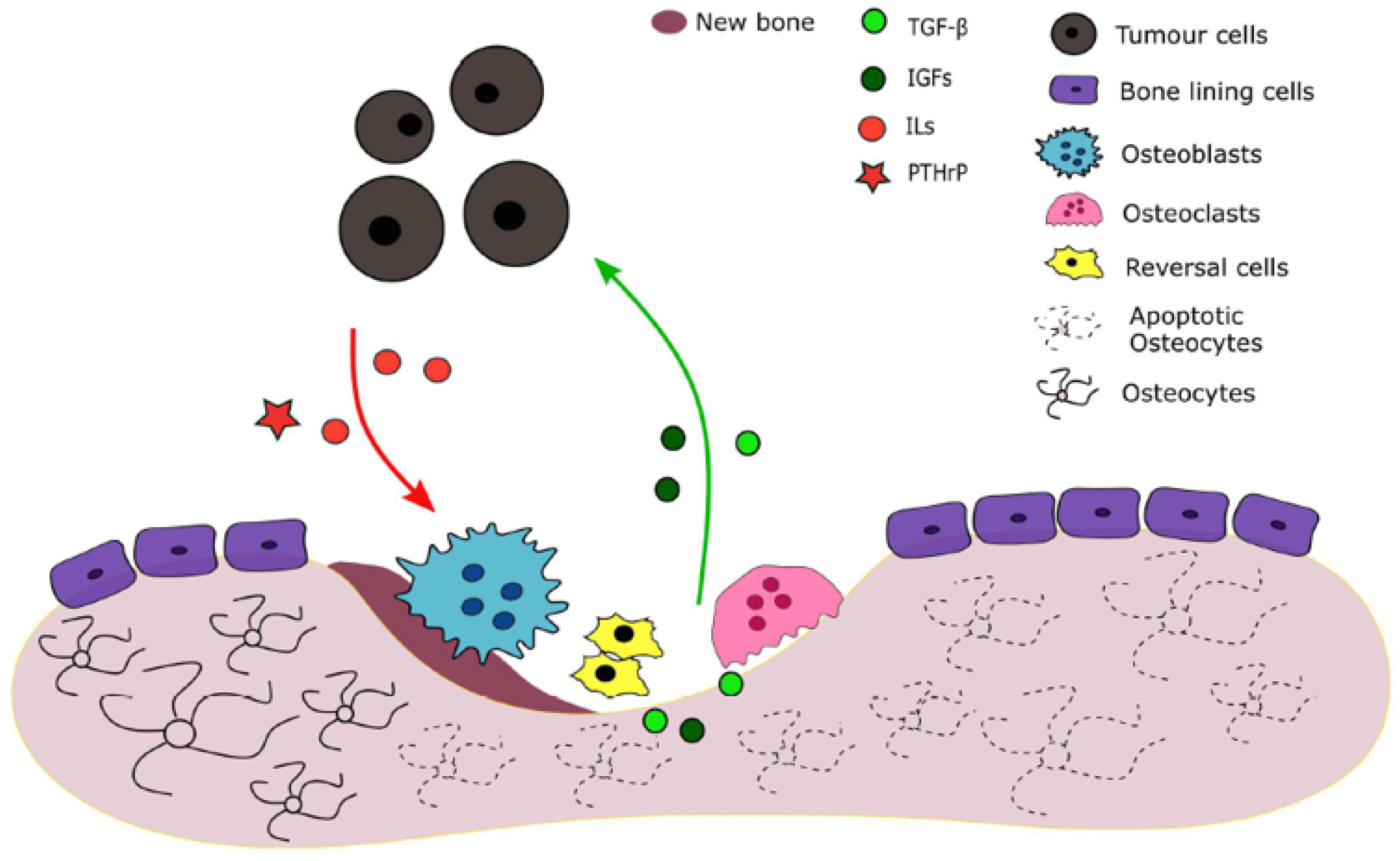
Tumour cells release several factors such as parathyroid hormone-related protein (PTHrP) and interleukins IL-6, IL-8 and IL-11 which promote osteolysis by stimulating osteoclast activity. A vicious cycle is established: factors that are trapped in the bone matrix and expressed during resorption, such as TGF-$\beta$, vascular endothelial growth factor (VEGF) and IGFs stimulate tumour cells’ survival and proliferation and subsequently PTHrP production. [11,13,14,15].

These interactions are graphically depicted in Figure 1. For more details about bone remodelling see, e.g., [16,17,18]; as to the effects of of tumours and their treatments, see, e.g., [19,20,21].

3. Proposed Models

3.1. Pharmacodynamics and Pharmacokinetics

The proposed bone remodelling and tumour growth model is based on Ayati’s [22] work. From that formulation, the therapy effects of four drugs were added: Denosumab ($T_1$), bisphosphonates or BP ($T_2$), Paclitaxel ($T_3$) and proteasome inhibitors or PI ($T_4$). The Pharmacokinectics, or PK (this designates the study of the time evolution of drug absorption, distribution, metabolism and excretion [23]), of each drug j is modelled as the two-compartmental model (1).

$$\frac{\mathrm{d}}{\mathrm{d}t}{C}_{g_j}\left(t\right)=-k_{a_j}{C}_{g_j}\left(t\right)$$

(1a)

$$\frac{\mathrm{d}}{\mathrm{d}t}{C}_{p_j}\left(t\right)=k_{a_j}{C}_{g_j}\left(t\right)-k_{e_j}{C}_{p_j}\left(t\right)$$

(1b)

The variable $C_g\left(t\right)$ is the concentration of the drug in a peripheral compartment, $C_p\left(t\right)$ is the effective concentration in plasma, $k_a$ is the absorption rate and $k_e$, the elimination rate [24].

The Pharmacodynamics, or PD (this refers to the relationship between drug concentration at the site of action and the resulting effect [25]), may be modelled with a Hill function (Equation (2)), whose output $d_j\left(t\right)$ is the drug effect in the system and lies within the interval $[0,1]$. The variable $C_{50}\left(t\right)$ is the concentration that achieves 50% of the drug’s maximum effect.

$$d_j\left(t\right)=\frac{C_{p_j}\left(t\right)}{C_{{50}_j}\left(t\right)+C_{p_j}\left(t\right)}$$

(2)

3.2. Finding the Bone Mass

The model equations relative to the OC number $C\left(t\right)$, OB number $B\left(t\right)$, bone mass $z\left(t\right)$ in percentage of its steady-state value, and tumour burden $T\left(t\right)$ in percentage of bone mass at time t [days] are represented by (3). The tumour growth is described with a gompertzian curve. Behind this equation lies the idea that the per capita growth of the population decreases exponentially with time. Its sigmoidal shape is qualitatively conceivable; the growth rate derivative of small sized tumours should be increasing, since they easily adapt to the environment obstacles. As the tumour increases in size, it the proliferation becomes more difficult, considering that the host physiology is more degraded, and the resources start to lack.

$$\frac{\mathrm{d}}{\mathrm{d}t}C\left(t\right)={\alpha }_{1}C{\left(t\right)}^{G_{11}}B{\left(t\right)}^{G_{21}}-({\beta }_1+K_{d_2}{d}_2\left(t\right))C\left(t\right)$$

(3a)

$$\frac{\mathrm{d}}{\mathrm{d}t}B\left(t\right)={\alpha }_{2}C{\left(t\right)}^{G_{12}}B{\left(t\right)}^{G_{22}}-({\beta }_2-K_{d_4}{d}_4\left(t\right))B\left(t\right)$$

(3b)

$$G_{11}=g_{11}(1+r_{11}\frac{T\left(t\right)}{L_T})$$

(3c)

$$G_{21}=g_{21}(1+r_{21}\frac{T\left(t\right)}{L_T})-K_{d_1}{d}_1\left(t\right)$$

(3d)

$$G_{12}=g_{12}/(1+r_{12}\frac{T\left(t\right)}{L_T})$$

(3e)

$$G_{22}=g_{22}(1-r_{22}\frac{T\left(t\right)}{L_T})$$

(3f)

$$\frac{\mathrm{d}}{\mathrm{d}t}z\left(t\right)=-k_{1}max[0,C\left(t\right)-\overline{C}]+k_{2}max[0,B\left(t\right)-\overline{B}]$$

(3g)

$$\frac{\mathrm{d}}{\mathrm{d}t}T\left(t\right)=\left({\gamma }_{tot}\right)T\left(t\right)log\left(\frac{L_T}{T\left(t\right)}\right)$$

(3h)

$${\gamma }_{tot}={\gamma }_T-K_{d_3}{d}_3\left(t\right)+K_{T}h\left(t\right)$$

(3i)

$$h\left(t\right)=max[0,C\left(t\right)-\overline{C}]$$

(3j)

The parameters ${\alpha }_i$ and ${\beta }_i$ are activities of cell production and removal, respectively. The index 1 refers to the OC population, and the index 2 to the OB. The autocrine and paracrine effects between OC and OB are not treated separately, their contributions are summed and expressed as the parameters $g_{ij}$, the net effectiveness of osteoclast or osteoblast-derived autocrine or paracrine factors. These can be positive (stimulatory) or negative (inhibitory).

The bone mass variation is attributed to the cell proliferation above the respective non-trivial steady-state levels, $\overline{C}$ (OC) and $\overline{B}$ (OB). The cells under this value are considered to be unable to resorpt or form bone, but they still participate in autocrine and paracrine signalling. The rates of bone formation and resorption are proportional to the number of osteoclasts and osteoblasts that exceed steady-state values, and $k_i$ represents the normalized activity of bone resorption ($i=1$) and formation ($i=2$). The parameter $L_T$ is an arbitrary value for the maximum size of $T\left(t\right)$ and ${\gamma }_T$ is the respective growth constant. The values r translate the effect of the metastasis size in the autocrine and paracrine factors. The term $h\left(t\right)$, given by (3j), is introduced in this work and represents the influence of an excessive osteoclastic activity in tumour proliferation. The parameter $K_T$ measures the effect of this influence.

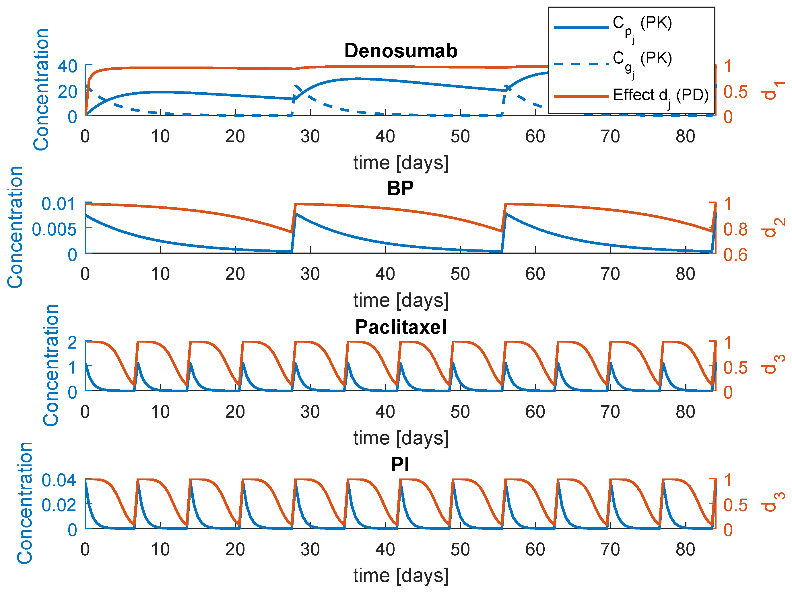
$K_{d_j}$ is the maximum effect of the drug $T_j$. The system (3) is a general representation that comprises the four drugs. In reality, these drugs are grouped in three combined therapies: $T_1+T_3$, $T_2+T_3$ and $T_4+T_3$. This means that there are only two inputs: the anti-cancer drug effect $d_3\left(t\right)$ and one of the three bone therapies effects, $d_1\left(t\right)$, $d_2\left(t\right)$ or $d_4\left(t\right)$. The PK/PD response is illustrated in Figure 2. The parameters of this simulation can be found in

Table 1. PK/PD parameters.

Parameter	Units	${\mathit{T}}_1$	${\mathit{T}}_2$	${\mathit{T}}_3$	${\mathit{T}}_4$
$C_{50}$	mg/L	1.2	0.0001	0.002	0.00005
$K_d$		0.09	0.005	0.015	0.002
$\tau$	day	4	4	1	1
$D_0$	mg	120	4	176	2.5
F		0.62	-	-	-
$V_d$	L	3.15	536.4	160.25	68.18
$k_a$	${\mathrm{day}}^{-1}$	0.2568	0	0	0
$k_e$	${\mathrm{day}}^{-1}$	0.0248	0.1139	1.2797	1.40

, including the periodicity of administration $\tau$. The PK/PD initial conditions for a single administration are obtained with $C_g^0=D_{0}F/V_d$, for $T_1$ and $C_p^0=D_0/V_d$, for the remaining drugs. The parameters $D_0$, $V_d$ and F correspond to the initial dose, volume distribution and bioavailability, respectively.

The PK/PD models and respective parameters regarding $T_1$, $T_2$ and $T_3$ were suggested by Coelho et al. [4]. The parameters regarding the PI model were estimated from a non-compartmental analysis in plasma of patients with advanced solid tumours, specifically the half life $t_{1/2}$ and estimated $C_p^0$ [26]. The remaining parameters of the model are fixed as: ${\alpha }_1=3$ ${\mathrm{day}}^{-1}$, ${\alpha }_2=4$ ${\mathrm{day}}^{-1}$, ${\beta }_1=0.2$ ${\mathrm{day}}^{-1}$, ${\beta }_2=0.02$ ${\mathrm{day}}^{-1}$, $k_1={7.48}^{-2}$ ${\mathrm{day}}^{-1}$, $k_2={5.52}^{-4}$ ${\mathrm{day}}^{-1}$, $g_{11}=1.1$, $g_{12}=1$, $g_{21}=-0.5$, $g_{22}=0$, $L_T=$ 100%, $K_T=4\times {10}^{-4}$, ${\gamma }_T=5\times {10}^{-3}$ ${\mathrm{day}}^{-1}$, $r_{11}=5\times {10}^{-3}$, $r_{12}=0.0$, $r_{21}=0.0$, $r_{22}=0.2$, $K_r=0.8$, $C_{{50}^{base}}=2\times {10}^{-3}$ mg/L, ${\lambda }_1={10}^{-6}$, ${\lambda }_2={10}^{-6}$, $C\left(0\right)=15$, $B\left(0\right)=316$, $z\left(0\right)=$ 100%, $T\left(0\right)=$ 0.001%, $\overline{C}=5$ and $\overline{B}=316$.

3.3. Inclusion of Drug Resistance

Model (3) diverges into two variations that approach the resistance to paclitaxel in two different manners, the models ${\mathrm{M}}_{DR1}$ and ${\mathrm{M}}_{DR2}$, each of them corresponding to a possible model of drug resistance found in the literature [24].

Model ${\mathrm{M}}_{DR1}$ considers that the resistance accumulation is caused by $C_p$ levels of the drug below a certain threshold $C_p^{th}$ [27]. The $C_{{50}_3}$ is affected according to

$$\begin{array}{cc}\hfill C_{{50}_3}\left(t\right)& =f\left(t\right)C_{50}^{base}\hfill \\ \hfill f\left(t\right)& =1+K_r{\int }_0^{t}max[0,C_p^{th}-C_p\left(\tau \right)]d\tau ,\hfill \end{array}$$

(4)

where parameter $K_r$ translates the capacity of the tumour cells to develop resistance and $C_{50}^{base}$ is a constant which represents the initial value of $C_{{50}_3}$.

Model ${\mathrm{M}}_{DR2}$ is based on the Random Mutation Model (RMM) [28], a Darwinian theory that proposes the existence of two proliferative tumour cell populations: $S\left(t\right)$ is composed completely sensitive cells, and $R\left(t\right)$ by completely resistant ones. The combination between the RMM and the proposed model (3) results in the following tumour growth description:

$$T\left(t\right)=R\left(t\right)+S\left(t\right)$$

(5a)

$$\frac{\mathrm{d}}{\mathrm{d}t}S\left(t\right)={\gamma }_{S}S\left(t\right)log\left(\frac{L_T}{T\left(t\right)}\right)+{\lambda }_{2}R\left(t\right)log\left(\frac{L_T}{T\left(t\right)}\right)$$

(5b)

$${\gamma }_S={\gamma }_T-K_{d_3}{d}_3\left(t\right)-{\lambda }_1+K_{T1}h\left(t\right);$$

(5c)

$$\frac{\mathrm{d}}{\mathrm{d}t}R\left(t\right)={\gamma }_{R}R\left(t\right)log\left(\frac{L_T}{T\left(t\right)}\right)+{\lambda }_{1}S\left(t\right)log\left(\frac{L_T}{T\left(t\right)}\right)$$

(5d)

$${\gamma }_R={\gamma }_T-{\lambda }_2+K_{T1}h\left(t\right),$$

(5e)

where ${\lambda }_1$ and ${\lambda }_2$ are the mutation and back-mutation rates between the S and R [29].

4. MPC–PSO scheme

4.1. Nonlinear Model Predictive Control

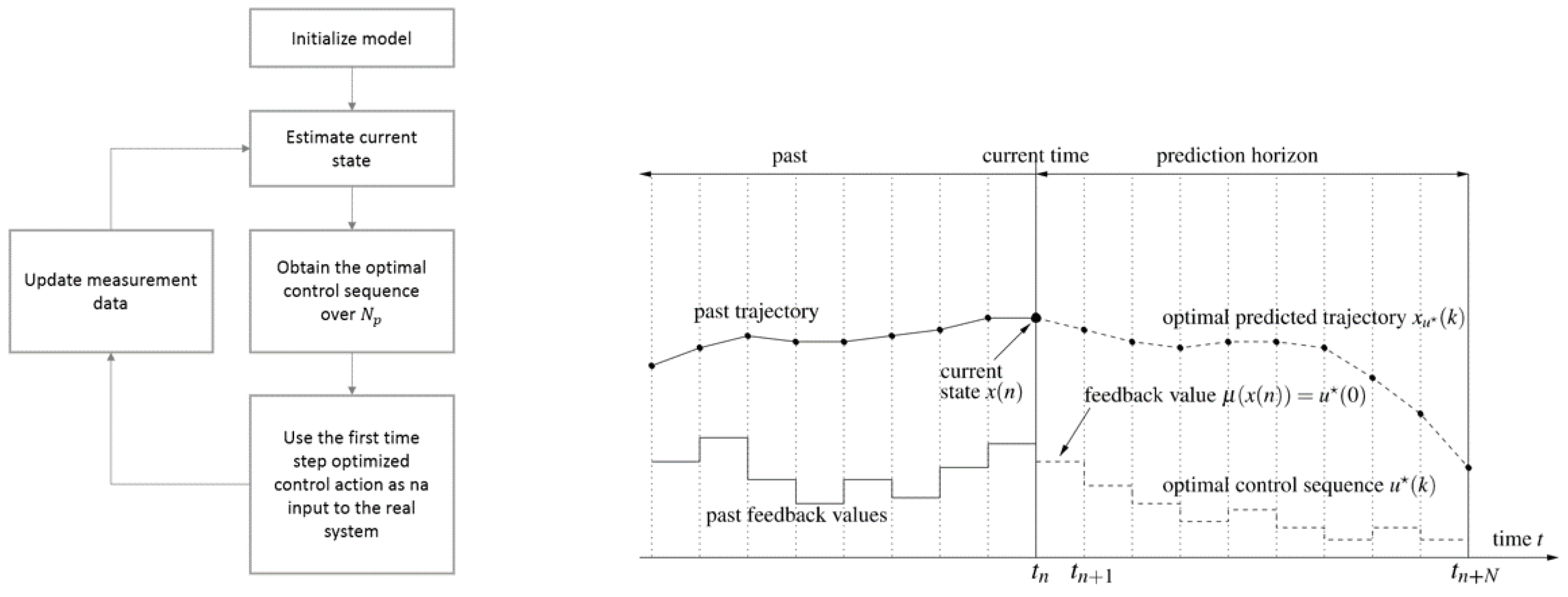
Model predictive control (MPC) refers to a class of control methods that make use of an an explicit process model to predict the future response of a system and obtain the control sequence over a certain horizon that minimizes a cost function. MPC performance is therefore highly dependent on the model performance. This also called receding horizon control does not allow the current time slot to be optimized, while keeping future time slots in account, which represents a major advantage; see Figure 3. The input is optimized for a finite prediction horizon $N_p$ and subsequently the first entries of the optimized input sequence (control horizon $N_c$) are fed back. It represents an advantage over classical control since it has the ability to explicitly account for systems constraints, the constrained nonlinear optimization problem is easy to formulate, multivariable processes can be handled in a straightforward manner, and reference tracking can be improved if the references are known in advance. Besides, it easily handles nonlinear and time-varying plant dynamics, since the controller is a function of the system and can be modified in real time [30,31]. The proposed implementation of NMPC in this work will count on metaheuristics, specifically Particle Swarm Optimization, to solve the nonlinear problem at each step. Combining metaheuristics with MPC brings flexibility to design any type of cost function.

4.2. Proposed PSO Algorithm

Particle Swarm Optimization (PSO) is a collective, anarchic, nature-inspired population-based search algorithm [32,33]. It is inspired in the social behaviour of a bird flock. PSO algorithms are a common choice to solve the optimization problem involved in model predictive control schemes [34,35].

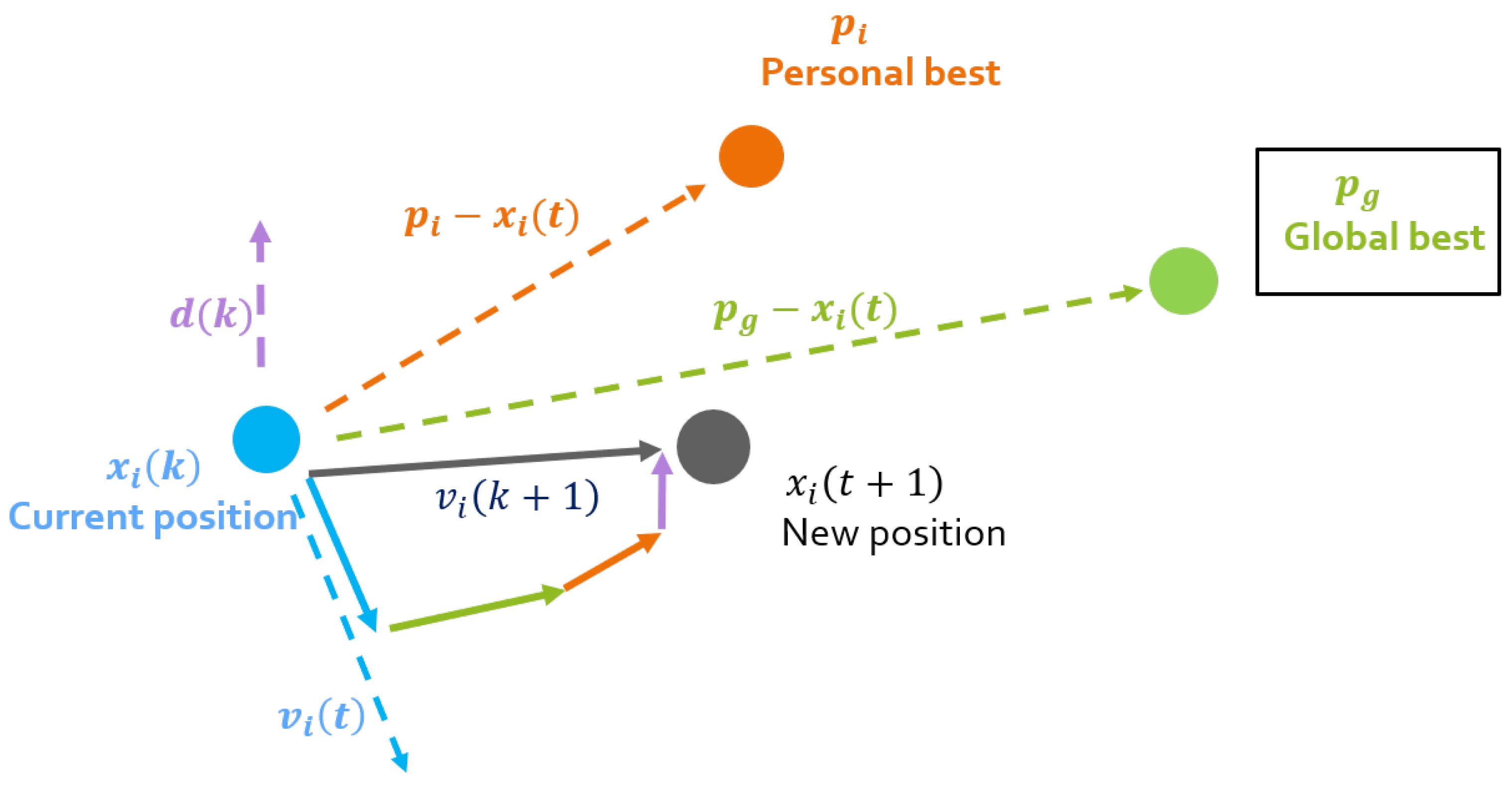
The swarm is composed by S particles wandering in a D-dimensional space. The position coordinates of each particle i are equivalent to a candidate solution. The particles’ position and velocity are updated taking into account advantageous positions of the surrounding partners. This position adjustment depends on the difference between the particles’ current position ${\mathbf{x}}_{\mathbf{i}}$ and two others: ${\mathbf{p}}_i$ (the best position visited by particle i, and ${\mathbf{p}}_g$ (the best position visited by any particle of the swarm). At each iteration k, the particles’ position and velocity vector ${\mathbf{v}}_{\mathbf{i}}$ are updated according to

$$\begin{array}{c}\hfill v_{ij}\left(k\right)=\chi \left[w_{ij}{v}_{ij}(k-1)+c_1\left(k\right){\mathrm{rand}}_1(p_{ij}-x_{ij}(k-1))+c_2\left(k\right){\mathrm{rand}}_2(p_{g_j}-x_{ij}(k-1))+c_3\left(k\right){\mathrm{rand}}_3{d}_{ij}\right]\end{array}$$

(6)

$$x_{ij}\left(k\right)=x_{ij}(k-1)+v_{ij}\left(k\right).$$

(7)

The acceleration/confidence parameters $c_1$, $c_2$ and $c_3$ are the cognitive, social and democratic coefficient, respectively. The particle’s inertia is measured by the inertia weight w and $\mathrm{rand}$ is a random number in the interval [0,1]. The last term is not present in the traditional PSO. This democratic approach brings to the velocity update the opinion of all eligible particles of the swarm [36]. The vector ${\mathbf{d}}_{\mathbf{e}}$ contains this swarm contribution and is obtained with

$${\mathbf{d}}_{\mathbf{e}i}=\sum _{k=1}^n{Q}_{ik}(x_{kj}-x_{ij})$$

(8a)

$$Q_{ik}=\frac{E_{ik}\frac{\mathrm{cost}\left(x_{best}\right)}{\mathrm{cost}\left(x_k\right)}}{{\sum }_{j=1}^n{E}_{ij}\frac{\mathrm{cost}\left(x_{best}\right)}{\mathrm{cost}\left(x_j\right)}}$$

(8b)

$$E_{ik}=\{\begin{array}{cc}1\hfill & \mathrm{if}\begin{array}{c}{\displaystyle \frac{\mathrm{cost}\left(x_k\right)-\mathrm{cost}\left(x_i\right)}{\mathrm{cost}\left(x_{worst}\right)-\mathrm{cost}\left(x_{best}\right)}>rand}\hfill \\ \wedge \mathrm{cost}\left(x_k\right)<\mathrm{cost}\left(x_i\right)\hfill \end{array}\hfill \\ 0\hfill & \mathrm{otherwise}\hfill \end{array},$$

(8c)

where $d_{ij}$ is the $j\mathrm{th}$ entry of vector ${\mathbf{d}}_{\mathbf{e}}$ for each particle i, $c_3$ is the confidence coefficient which controls the weight of the the democratic quantities, and $\mathrm{cost}\left(x\right)$ is the cost function chosen for the particular problem evaluated at x. This vector represents the democratic effect of the other particles in the movement of particle i. The weight of the kth particle is represented by $Q_{ik}$, which depends on the eligibility parameter $E_{ik}$. The best and worst particles of the swarm at each iteration are denoted $x_{best}$ and $x_{worst}$, respectively.

The adaptive profile of the proposed algorithm, AD-PSO is translated in the inertia weight evolution with the iterations [37]. The inertia weight value regarding the $j\mathrm{th}$ variable of the particle i is updated with the Equations (9) and (10).

Value $w_0$ is a constant that defines the initial inertia weight. Parameter $ϵ$ is a non-critical small and positive value that ensures a proper variation of the inertia weight. Value $\Lambda$ is obtained with (10), where $ϵ$ is a non-critical small and positive value that ensures a proper variation of the inertia weight.

$$w_{ij}(k+1)=\{\begin{array}{cc}min\left(1,w_{ij}\left(k\right)+(1-w_0)e^{\Lambda }+ϵ\right)\hfill & \mathrm{if}{\delta }_i\left(k\right)>0\wedge {\delta }_i(k-1)>0\hfill \\ max(0.1,w_{ij}\left(k\right)-w_0\left(\left(1-e^{\Lambda }\right)-ϵ\right)\hfill & \mathrm{if}{\delta }_i\left(k\right)<0\wedge {\delta }_i(k-1)<0\hfill \\ w_{ij}\left(k\right)\hfill & \mathrm{otherwise}\hfill \end{array}$$

(9)

$$\Lambda =\frac{{(x_{ij}(k+1)-p_{ij}\left(k\right))}^2}{-2{\sigma }^2}$$

(10)

The values ${\delta }_i$ measure the success of particle i in the following manner:

$${\delta }_i=\{\begin{array}{cc}1\hfill & \mathrm{if}\mathrm{cost}\left({\mathbf{x}}_1\right)<\mathrm{cost}\left({\mathbf{p}}_i\right)\hfill \\ -1\hfill & \mathrm{otherwise}\hfill \end{array}$$

(11)

The TVAC algorithm (Time Varying Acceleration Coefficients) [38] dictates the dynamic behaviour of both $c_1$ and $c_2$ according to Equations (12).

$$c_1\left(k\right)=(c_{1_f}-c_{1_i})\frac{k}{n_{iter}}+c_{1_i}$$

(12a)

$$c_2\left(k\right)=(c_{2_f}-c_{2_i})\frac{k}{n_{iter}}+c_{2_i}$$

(12b)

The values $c_{i_1}$ and $c_{f1}$ are the initial and final values of the coefficient $c_1$ while $c_{i2}$ and $c_{f2}$ represent the initial and final values of $c_2$. These linearly increasing and decreasing behaviours are defined until the maximum number of iterations $n_{iter}$.

The minimum number of $n_{iter}$ is set to $n_{iter}=100$, however the algorithm stops when a state of convergence is achieved. The stopping criterion uses a counter $\theta$ which records the number of consecutive iterations with no improvement, after $k>n_{iter}$, according to (13). The algorithm stops when $\theta$ reaches a maximum value ${\theta }_{max}$.

$$\theta \left(k\right)=\{\begin{array}{c}{\displaystyle 0,\hspace{1em}\hspace{1em}\mathrm{if} \mathrm{cost}\left(p_g\left(k\right)\right)<\mathrm{cost}\left(p_g(k-1)\right)\vee k<n_{iter}}\hfill \\ \theta (k-1)+1,\hspace{1em}\hspace{1em}\mathrm{otherwise}\hfill \end{array}$$

(13)

The dynamic parameters are maintained constant at $c_1\left(k\right)=1.5$ and $c_2\left(k\right)=2.5$ for $k>n_{iter}$.

The PSO parameters were fixed for this problem as: $S=50$, $w_0=0.9$, $ϵ=0.005$, $c_{1_i}=c_{2_f}=2.5$, $c_{2_i}=c_{1_f}=1.5$, ${\theta }_{max}=15$. The algorithm is depicted in Figure 4.

5. Implementation

In this section, the NMPC-PSO scheme described in Section 4 is implemented with the objective of optimizing the prescription doses of the proposed therapies, when the drugs are administered with the fixed periodicity $\tau$.

Only the therapies $T_1+T_3$ and $T_4+T_3$ are considered for this optimization. The BP therapy, although it results in a qualitatively viable therapy model, is not suitable for optimization. The rise of OC apoptosis due to BP decreases, although very slightly, the lower bound of the OC time response. The tumour $T\left(t\right)$ causes the opposite reaction: an increase of the mean value of $C\left(t\right)$, as well as its lower bound. When the tumour is proliferating, or has a substantial size, this lower bound increase cancels out the decrease caused by BP. When the tumour starts to be extinguished, the anti-resorptive effect pushes the OC number to fall below zero. Although the negative values of OC are smaller orders than $\overline{C}$, it is enough to severely interfere with the dynamics, due to the appearance of complex numbers.

The standard regimen is defined as the prescription schedule which administrates constant values of $C_p^0$ and $C_g^0$. The decision variables are $C_p^0$, for the initial concentration of paclitaxel and PI and $C_g^0$ for the initial concentration for denosumab. These values for the initial concentration are fixed at $C_{g1}^0=23.62$, $C_{p4}^0=0.0367$ and $C_{p3}^0=1.0983$ (denosumab, PI and paclitaxel, respectively). The lower bound of the concentration is equal to zero for all drugs and the upper bound is considered to be three times the standard regimen doses, and therefore $C_{p{1}_{max}}^0=70.86$, $C_{p{4}_{max}}^0=0.11$ and $C_{p{3}_{max}}^0=3.29$. The maximum velocity of the particles, ${\mathbf{v}}_{\mathbf{max}}$ is calculated offline as ${\mathbf{v}}_{\mathbf{max}}=0.2({\mathbf{x}}_{\mathbf{max}}-{\mathbf{x}}_{\mathbf{min}})$ and the minimum as ${\mathbf{v}}_{\mathbf{min}}=-{\mathbf{v}}_{\mathbf{max}}$. The time of the diagnosis and therefore the beginning of the optimization is considered to be $t_{start}=800$ days. The optimization is single-objective and the goal is to minimize the tumour size, the drug dosage and approximate the bone mass to a healthy level as much as possible. The objective function is defined as

$$\begin{array}{cc}\hfill J=& w_1{\mathbf{D}}_t^{-1}{(1-\frac{z\left(t\right)}{L_1})}^2+w_2{\mathbf{D}}_t^{-0.8}\frac{T\left(t\right)}{L_2}\hfill \\ \hfill & +w_3{\mathbf{D}}_t^{-1}\frac{C_{p_{br}}\left(t\right)}{L_3}+w_4{\mathbf{D}}_t^{-1}\frac{C_{p_3}\left(t\right)}{L_4},\hfill \end{array}$$

(14)

where $C_{p_3}$ and $C_{p_{br}}$ are the plasma concentration evolutions of paclitaxel and one of the two bone remodelling pharmaceuticals, $C_{p_1}$ or $C_{p_4}$. The quantities $L_1$, $L_2$, $L_3$ and $L_4$ are maximum values of z, T, $C_{p_{br}}$ and $C_{p3}$, respectively and can be found in

Table 2. Parameters of the objective function.

i	1	2	3		4
			Den.	PI
$L_i$	100	100	3.29	0.11	70.86
$w_i$	4	15	0.5	1	1

, as well as the weights $w_1$, $w_2$, $w_3$ and $w_4$. The functional operator $D^{-1}$ is a Riemann integral, and $D^{\alpha }$ is a fractional derivative, defined here (according to Grünwald and Letnikoff) as [39]

$${}_{c}D_t^{\alpha }f\left(t\right)=\underset{h\to 0^{+}}{lim}\frac{{\sum }_{k=0}^{\left[\frac{t-c}{h}\right]}{(-1)}^k\left(\genfrac{}{}{0pt}{}{\alpha }{k}\right)f(t-kh)}{h^{\alpha }},$$

(15)

where $\left(\genfrac{}{}{0pt}{}{a}{b}\right)$, the combinations of a things, b at a time can be obtained with [40]

$$\left(\genfrac{}{}{0pt}{}{a}{b}\right)=\{\begin{array}{cc}\frac{\Gamma (a+1)}{\Gamma (b+1)\Gamma (a-b+1)}\hfill & \mathrm{if} a,b,a-b\notin {\mathbb{Z}}^{-}\hfill \\ \frac{{(-1)}^b\Gamma (b-a)}{\Gamma (b+1)\Gamma (-a)}\hfill & \mathrm{if} a\in Z^{-}\wedge b\in {\mathbb{Z}}_0^{+}\hfill \\ 0\hfill & \mathrm{if} [(b\in {\mathbb{Z}}^{-}\vee b-a\in \mathbb{N})\wedge a\notin {\mathbb{Z}}^{-}]\vee (a,b\in {\mathbb{Z}}^{-}\wedge a>b).\hfill \end{array}$$

(16)

$\Gamma$ is the gamma function, an extension of the factorial function.

A fractional derivative was used here because we are interested in attributing a weight to tumour level that increases with time; therefore, the functional order is set to $n=-0.8$, instead of order $n=-1$, which corresponds to a classical integrator and weights all past moments equally [40].

6. Results

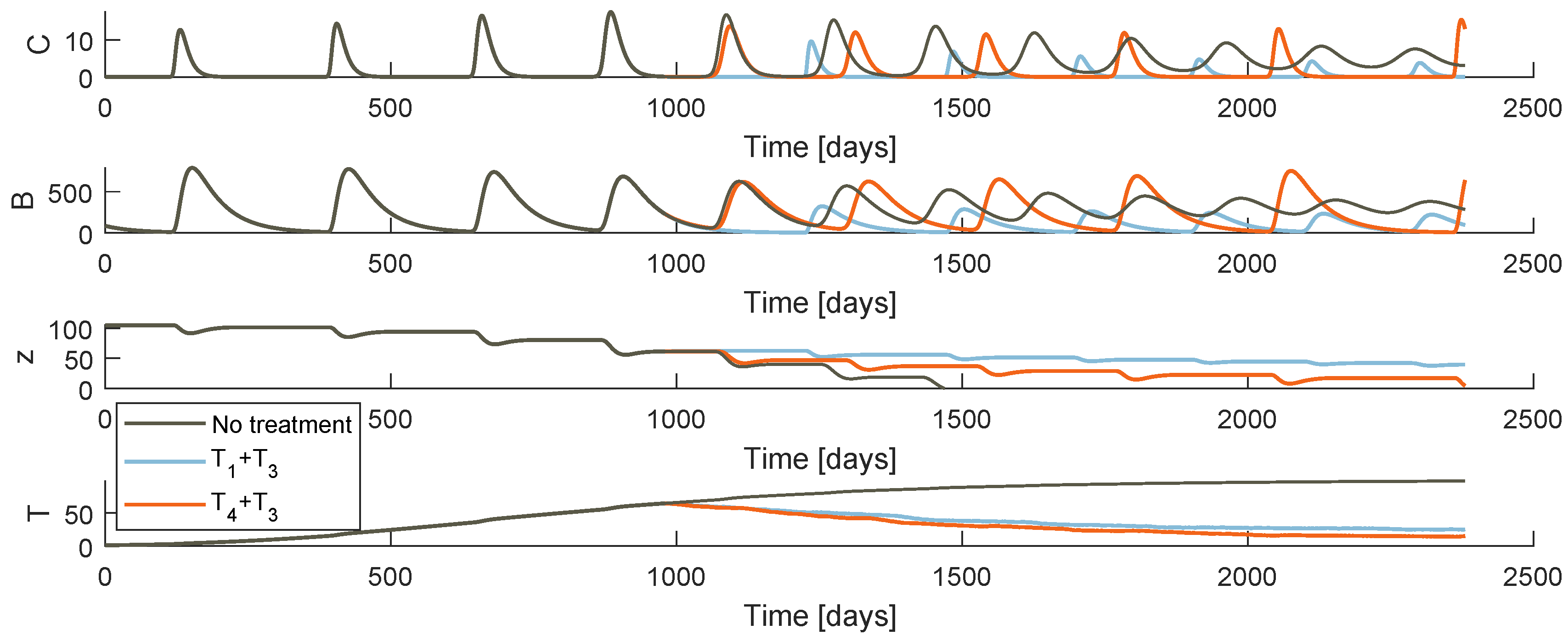
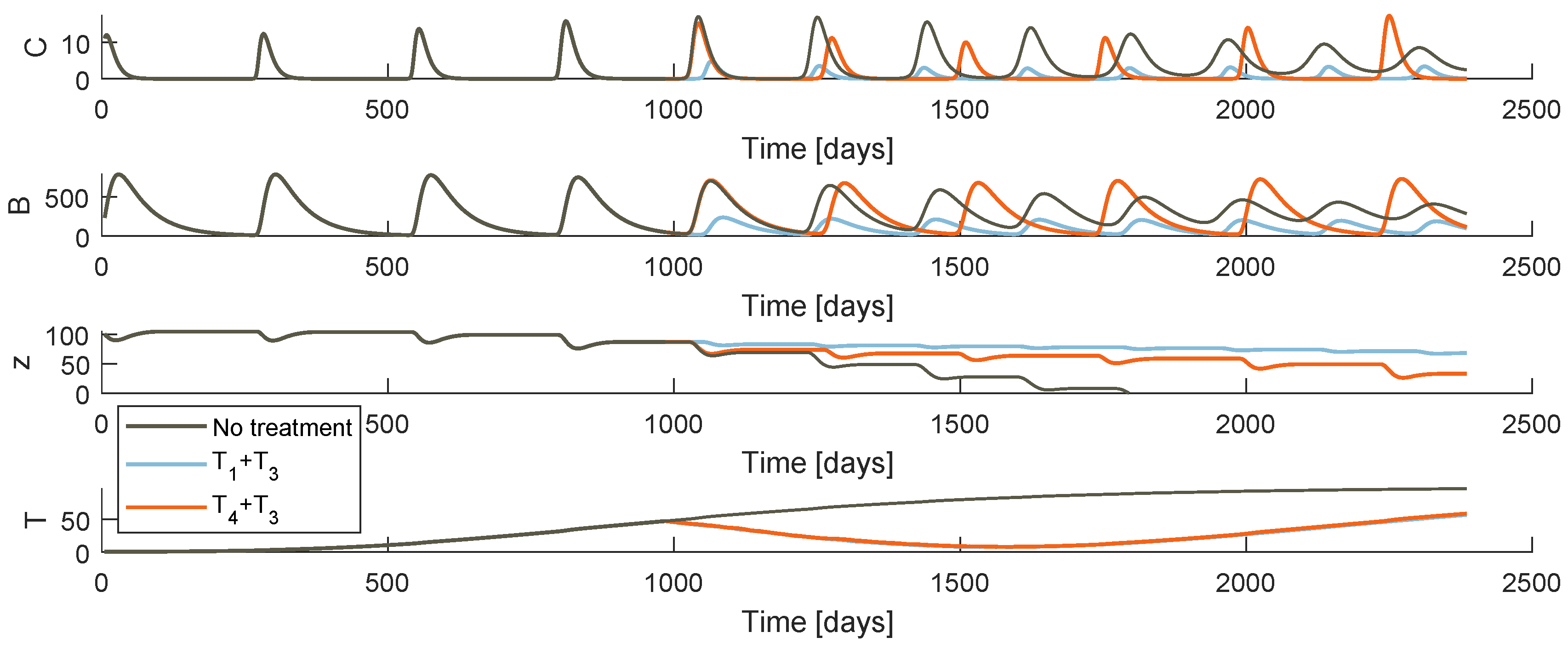
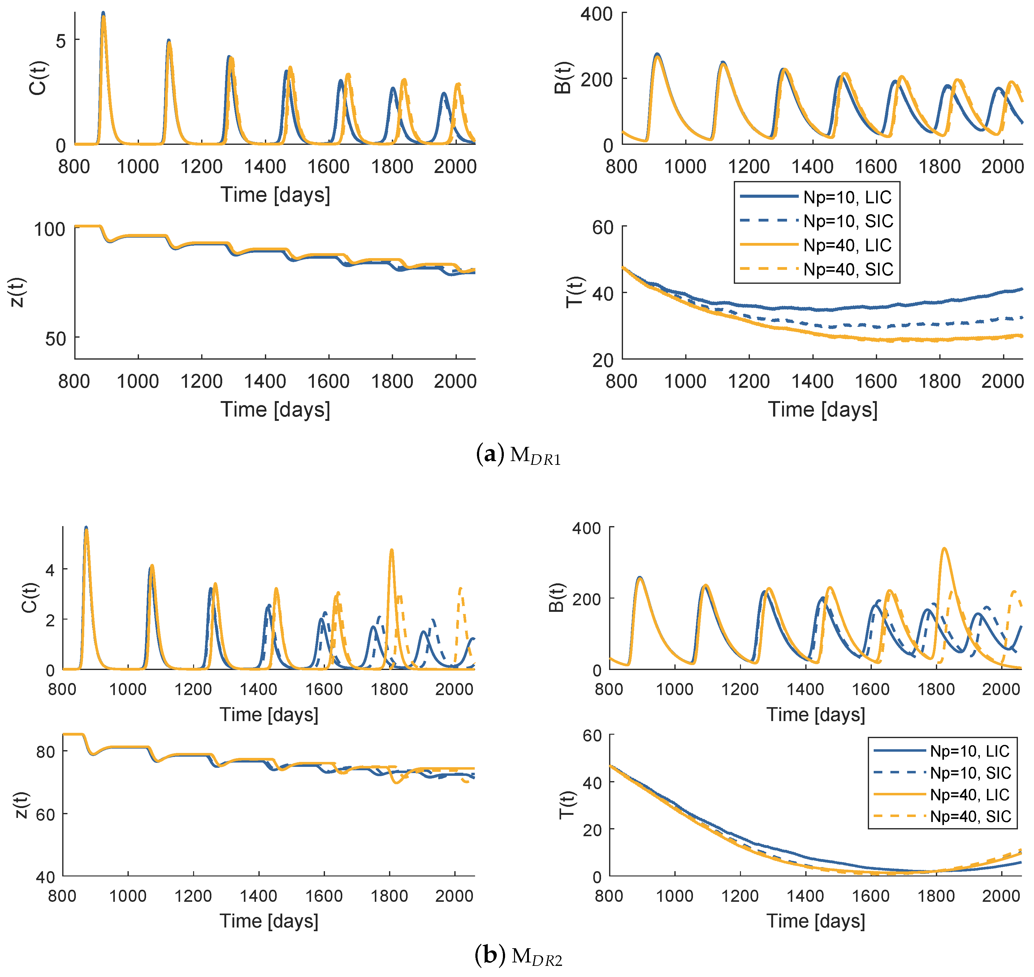
Figure 5 and Figure 6 plot the system behaviour of models ${\mathrm{M}}_{DR1}$ and ${\mathrm{M}}_{DR2}$, respectively, when each of the therapies are administrated. At first glance, both models under the therapies $T_1+T_3$ an $T_4+T_3$ appear to have a similar qualitative behaviour. Comparing the bone resorption therapies (PI or denosumab), there are clear differences specially when it comes to the OC and OB oscillatory behaviour. The different type of action of both drugs justifies these discrepancies. One should not make comparison assumptions of these pharmaceuticals solely based on these simulations: the fact that $z\left(t\right)$ stabilization is more effective under a certain model may be due to the chosen system parameter values.

Regarding the different drug resistance models, the tumour growth behaviour is different depending on whether the phenomenon is modelled under the random mutation or the varying $C_{50}$ model. Both models predict a decrease of T immediately after the therapy starts, more or less symmetric to the precedent increase for a few weeks. The tumour achieves then a low value that never reaches 0. In model ${\mathbf{M}}_{DR2}$, the drug resistance effects arise when the resistant population uncontrollable proliferation continues with the same strength as the initial cancer, after an apparent remission. As soon as the gradient turns positive, it is certain that the metastasis will grow abruptly to high values until death. On the other hand, model ${\mathbf{M}}_{DR1}$ allows a smoother accumulation of resistance. Even if the tumour does not reach values as low as with the last model, the cancer is maintained at a more constant value after the point when drug resistance is evident.

6.1. Model $M_{DR1}$—Therapy $T_1+T_3$

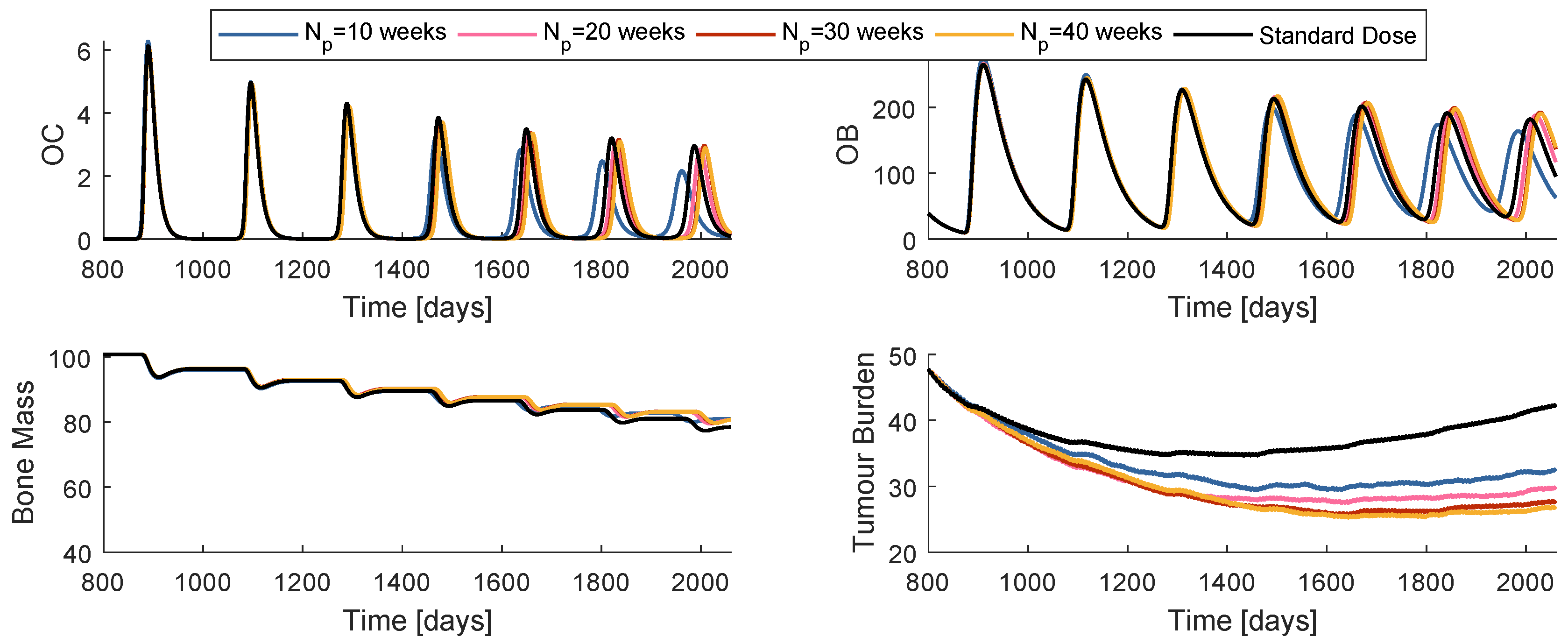
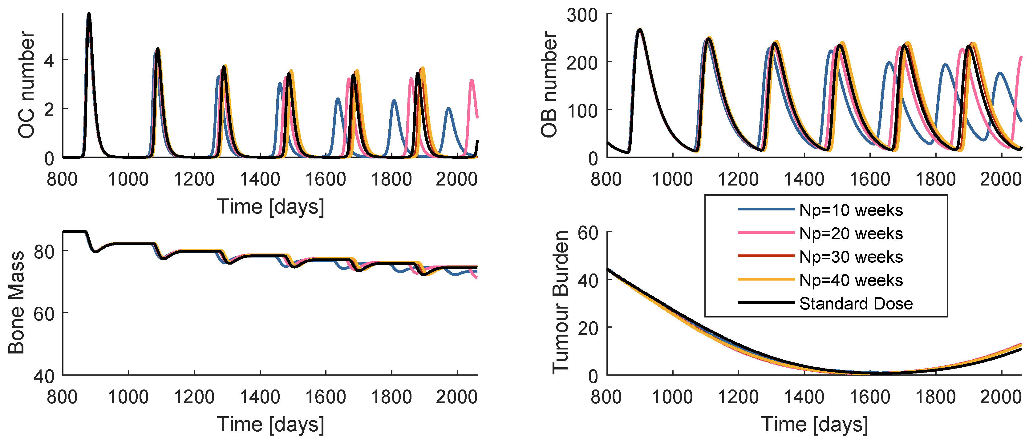
While the control horizon $N_c$ was maintained constant, the prediction horizon $N_p$ was varied between 10, 20, 30 and 40 weeks. The $N_c$ is fixed to 4 weeks. The global best position ${\mathbf{p}}_g$ is initialized with the dose values of standard regimen, a strategy that from now on will be termed SIC (standard initial condition). Figure 7 is a comparison of the system reaction to the best obtained prescription when $N_p=10$, $N_p=20$, $N_p=30$, $N_p=40$ and when the prescription is standard. The cost decreases with the increase of $N_p$, when handling the model ${\mathrm{M}}_{DR1}$. Nevertheless, all of the four prescriptions are more successful than the standard regimen.

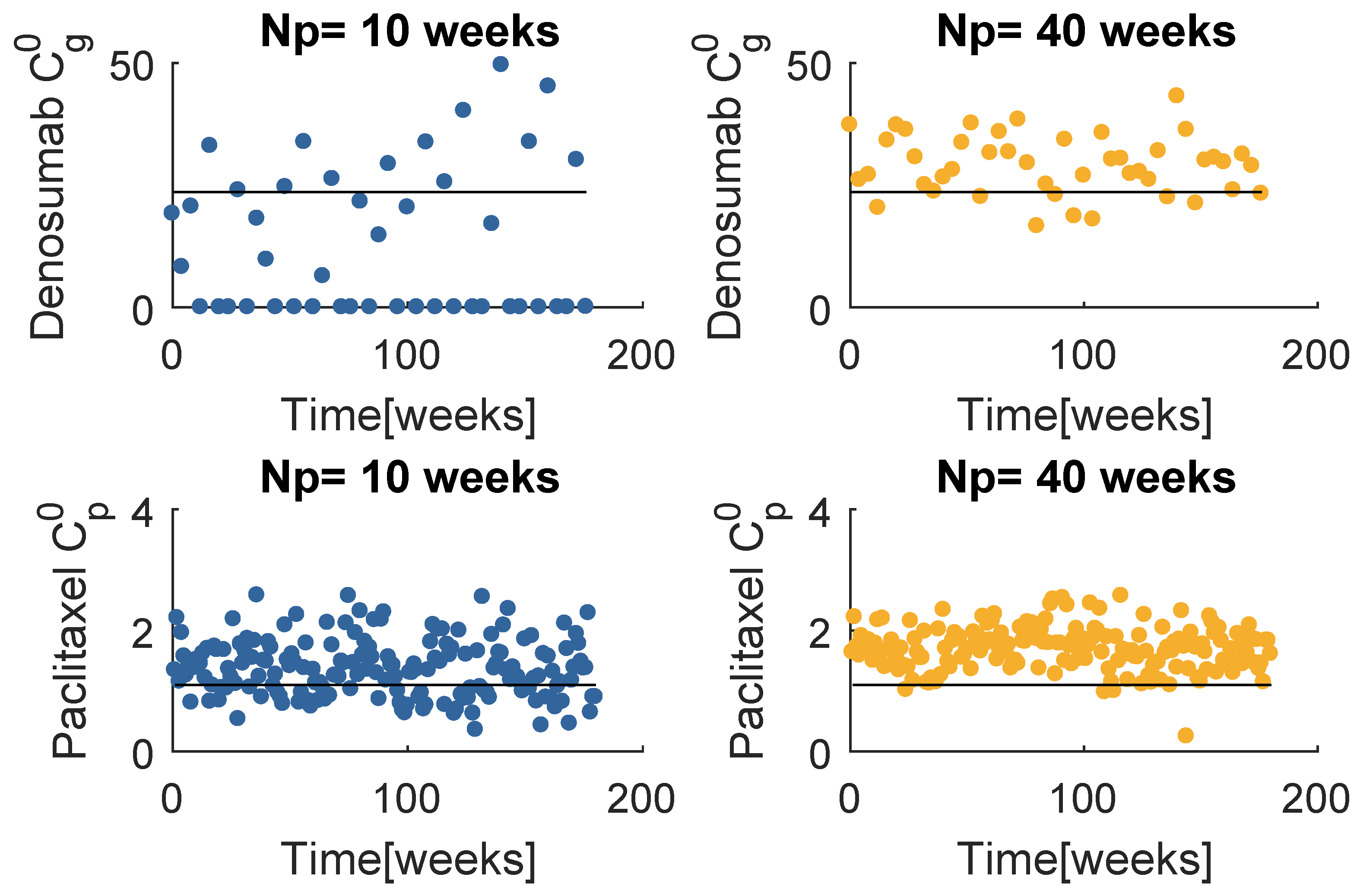
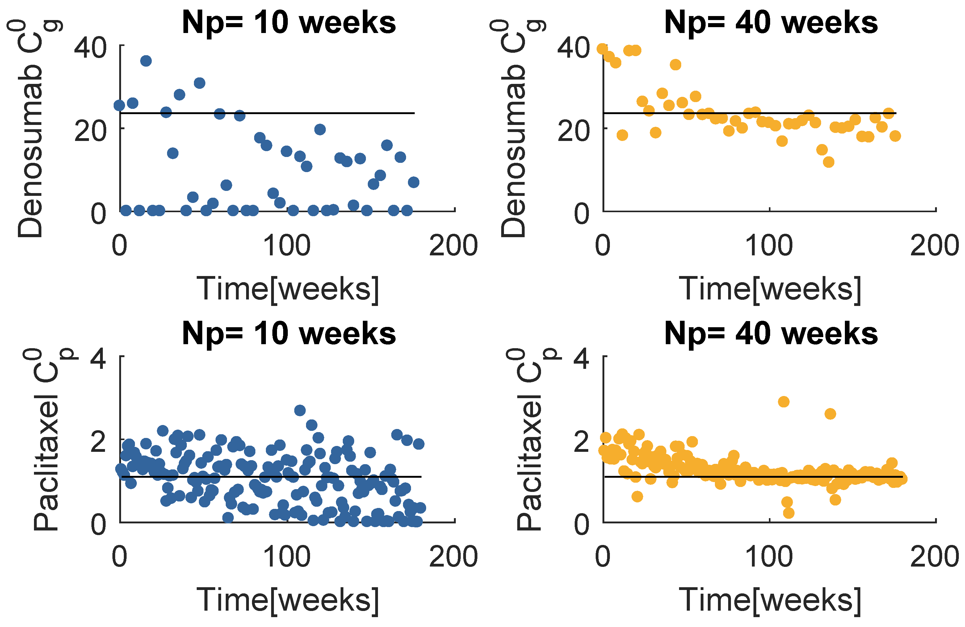
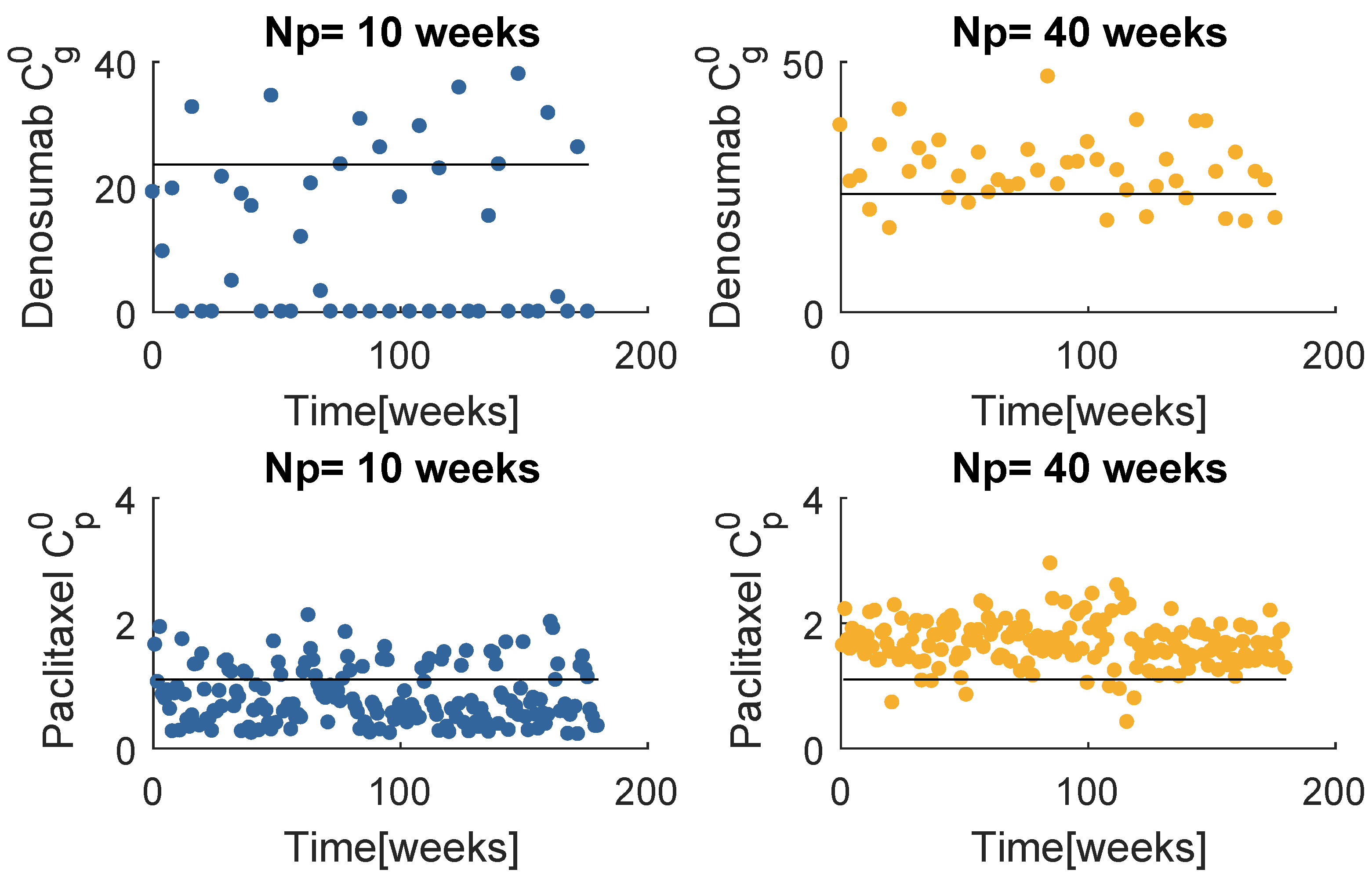
Figure 8 contains the resultant prescription of denosumab and paclitaxel with the model ${\mathrm{M}}_{DR1}$, when $N_p=10$ and $N_p=40$. The $C_p^0$ and $C_g^0$ mean values tend to coincide with a value higher than the respective standard dose, yet lower than the maximum values defined for this problem. Note that when $N_p=10$, MPC obtains several null entries (22 out of 45 administrations), suggesting a higher $\tau$ for the denosumab. The increase in $N_p$ tends to produce a drug concentration distribution less variant.

6.2. Model $M_{DR2}$—Therapy $T_1+T_3$

The two populations model, ${\mathbf{M}}_{DR2}$, was subject to the same sensitivity analysis. The system dynamics when $N_p$ is fixed to different values is compared in Figure 9. The almost indistinguishable curves translate the insensitivity of the model to $N_p$. This model allows a decrease of the tumour size to almost null values; however, when the resistance effects arise, the regrowth is extremely aggressive. The impossibility of tumour annihilation is associated with a resistant and proliferative population. Therefore, the resistance can never be defeated with a unique anti-cancer drug.

The denosumab and paclitaxel prescription results are shown in Figure 10. From these plots it is verified that the paclitaxel is administrated even after the sensitive population is supposedly extinguished. One might suspect that this administration would be interrupted at some point, since it has no effect on the resistant population. In fact, the doses diminish over time, but they never reach 0. This is due to the nature of the Gompertz equation: the sensitive population never actually reaches full extinction, just residual values. Besides, the S population keeps acquiring part of the resistance cells that suffer back-mutation. Therefore, there is a necessity of a paclitaxel continuity to keep the S population from regrowth. The outcome from the optimization when $N_p=10$ suggests a higher ${\tau }_1$ of denosumab, as it happened with ${\mathrm{M}}_{DR1}$.

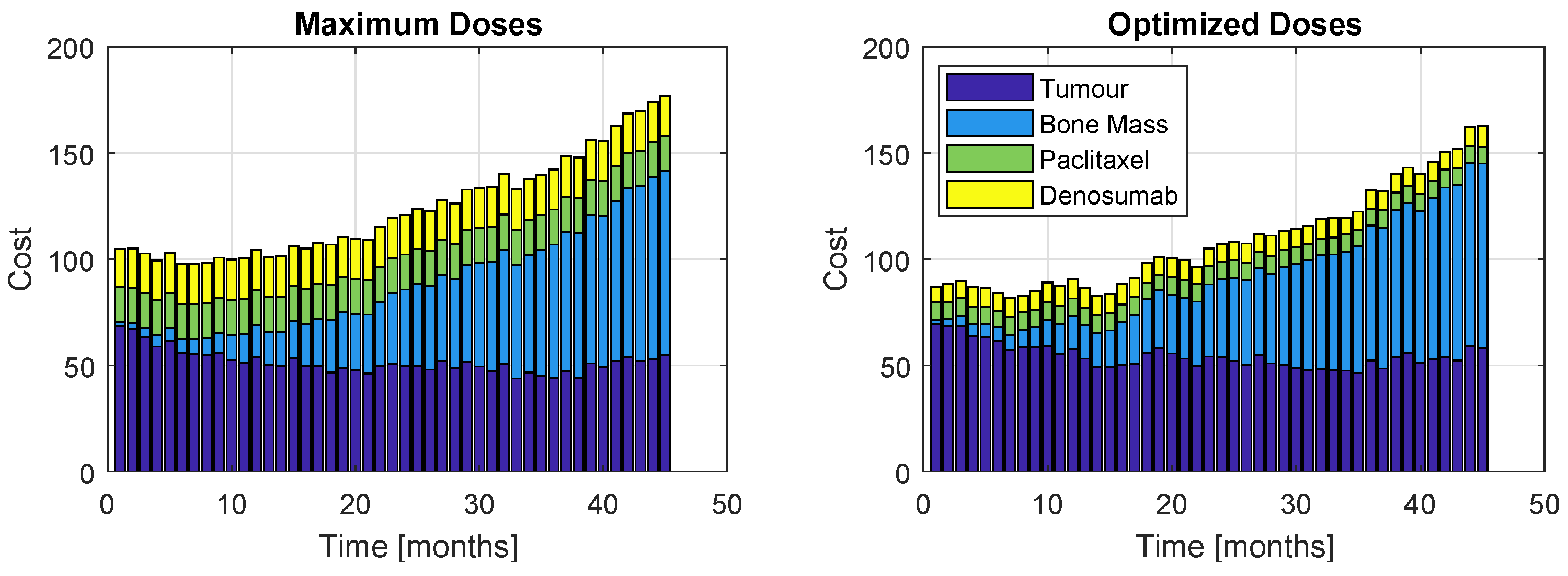
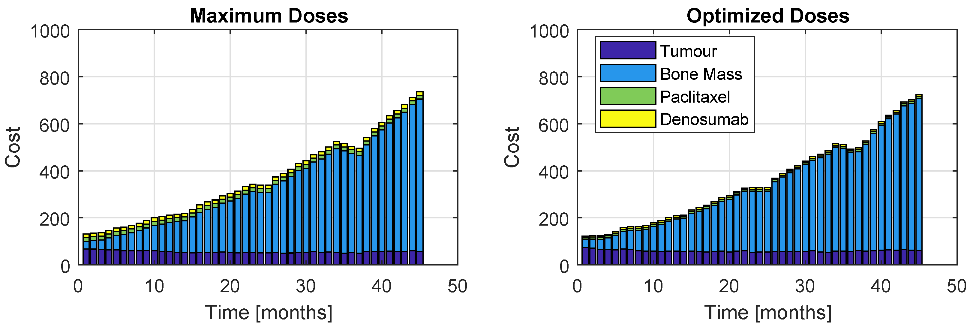
Although the algorithm accounts for one single cost, the proportions of each term of the objective function throughout the 45 months of treatment is displayed in Figure 11 (Model ${\mathbf{M}}_{DR1}$) and Figure 12 (Model ${\mathbf{M}}_{DR2}$). The left plots correspond to a patient who received the maximum dose allowed for this problem, while the right plots correspond to prescription resultant from optimization. As expected, the administration of the maximum allowable doses retrieve slightly better values for the tumour and bone mass associated cost; however, the inherent high administration cost does not allow this prescription to be a good option. Nevertheless, the optimization prescription outputs extremely close tumour and bone mass costs (in fact, almost indistinguishable) to those obtained with the most aggressive therapy. This represents a major advantage, since the patient is safeguarded from a therapy with higher drug exposure, but still obtaining very similar results.

6.3. Therapy $T_4+T_3$

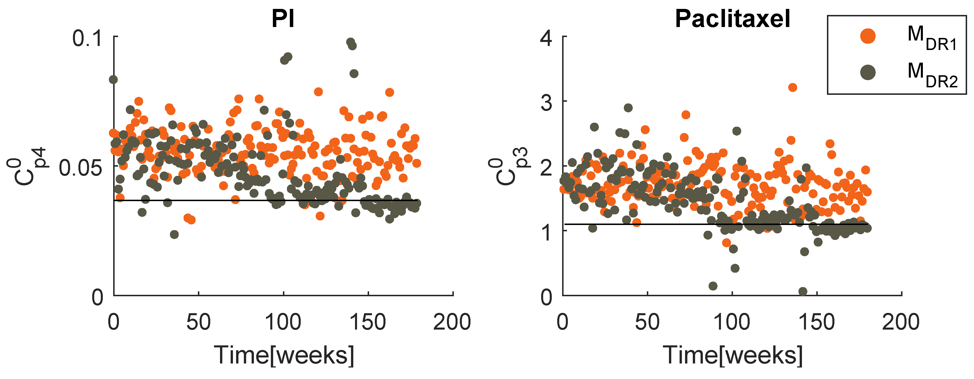
When handling the therapy $T_4+T_3$, the PSO deals with problems with higher dimensions, because $T_4$ has a more frequent administration than $T_1$. To avoid excessive computational effort, the optimization of this therapy was performed only once for each model, with $N_p=40$ weeks. Figure 13 presents the best obtained prescriptions of PI and paclitaxel, for both models. As expected, the $C_p^0$ evolutions follow a similar pattern to that of the last therapy. When handling model ${\mathrm{M}}_{DR1}$, a mobile mean value of both drugs is maintained almost constant, as well as the standard deviation. When facing a two populations model, a decreasing tendency is evident for both dose value and standard deviation. In both therapies, $C_{p_3}^0$ converge to similar values.

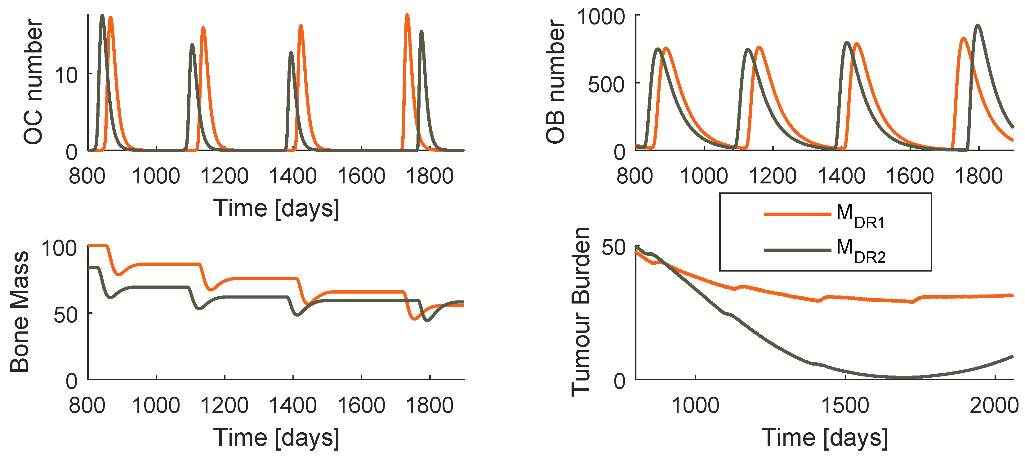
The system dynamics when the optimized regimen is applied is shown in Figure 14 for both models. The amplitude of oscillation of OC and OB is significantly higher when PI is used instead of denosumab, as the respective period.

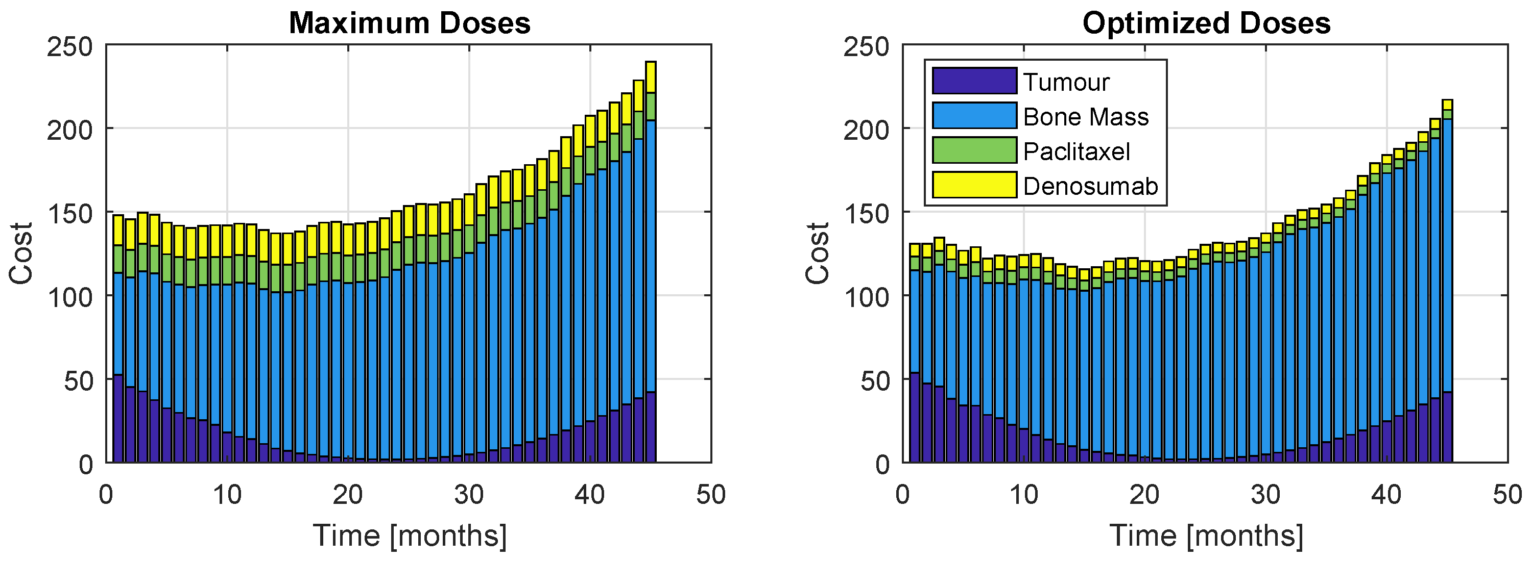
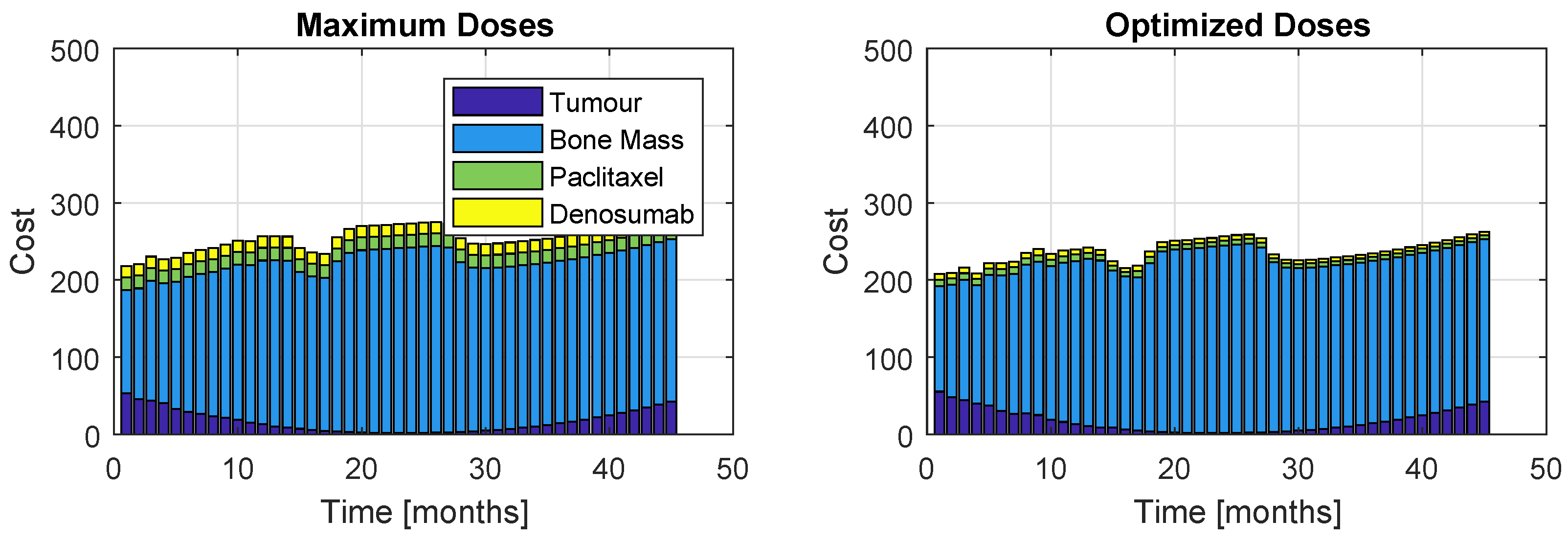
The cost proportions are once again represented, in Figure 15 and Figure 16, for the models ${\mathrm{M}}_{DR1}$ and ${\mathrm{M}}_{DR2}$, respectively. As before, the left plots refer to a patient who took maximum doses of both drugs and the right plots to a patient whose regimen was optimized. Figure 15 shows a similar increasing evolution to Figure 11, although the costs are considerably higher and there is a bigger discrepancy between the proportion of the weight related to the bone mass to the rest of the terms of J. Figure 14 and Figure 16 reinforce the impossibility of avoiding a U-shaped tumour curve when dealing with ${\mathrm{M}}_{DR2}$. The oscillating appearance of the curves of Figure 16 is due to the extremely high period and amplitudes that PIs provoke in the bone remodelling process.

6.4. Sensitivity to the Initial Global Best Position

The dependency of the optimization regarding the initial global best position is here analysed. The strategy SIC is replaced by the strategy LIC (low initial condition), which initializes ${\mathbf{p}}_{\mathbf{g}}$ with concentration values that are ten times smaller than the standard regimen’s. This section compares both strategies.

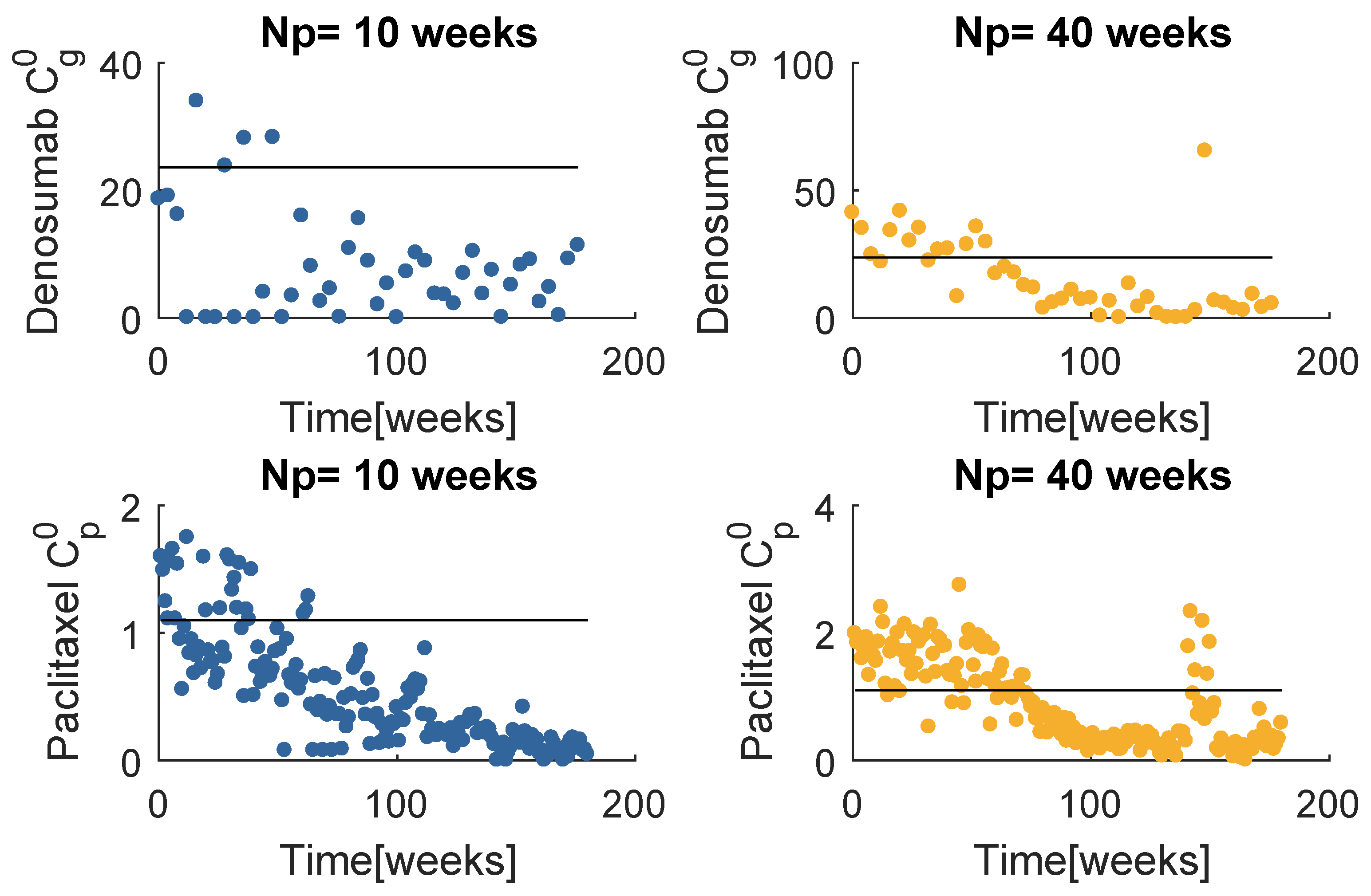
The prescription doses with LIC (Figure 17) appear not to have changed significantly, when compared with SIC (Figure 8). The only significant difference between these results is the paclitaxel administration when $N_p=10$. The considerably lower doses resulted in poorer performance treating the tumour burden when compared to a standard initial condition, as one can verify in Figure 18a.

When handling ${\mathrm{M}}_{DR2}$, the resultant prescriptions differences are much more pronounced (Figure 19). All of the dose values decrease with time, and this variation is significantly more accentuated with a low initial global best position, of both denosumab and paclitaxel. In fact, approximately in the last two thirds of the treatment period, almost all of the doses are far below the standard values. The input sequences obtained with SIC and LIC, although very disparate, produced quite similar results on the system behaviour (Figure 18b). The PSO fitness values evaluated when LIC is used are about $10\%$ lower than those obtained with SIC when $N_p=40$ but are almost equal when $N_p=10$. The tumour decrease with the LIC prescription when $N_p=10$ is not so fast, however the regrowth due to resistance is slightly postponed. Although this result translated in a higher cost associated to the tumour, the interpretation would be different if one attributed more importance to the late regrowth. In fact, this particular result supports the paradigm that says that the resistant population is delayed if the sensitive is not immediately eradicated.

One concludes that the optimization resultant input sequence with the model ${\mathrm{M}}_{DR2}$ is very sensitive to the initial global best position, contrarily to ${\mathrm{M}}_{DR1}$. It seems more favourable to start the global best to lower values, since the significant lower prescription doses are still enough to produce the same results as the SIC strategy. This analysis was not performed with the therapy $T_4+T_3$ due to the excessive computational effort, but it is fair to generalize this conclusion.

7. Conclusions

The proposed model contains two major novelties: (1) the positive influence of the osteoclasts activity in the tumour proliferation, in order to recreate a vicious cycle between the two mechanisms, and (2) two drug resistance mechanisms regarding the immunity of tumour cells to paclitaxel, according to two different paradigms on the topic. The PK/PD of four drugs (Denosumab, BP, paclitaxel and PI) were included to simulate more accurately the system reaction to the therapy. Several factors regarding the OC and OB coupling and survival are yet to be considered and included in a more meticulous description of the system.

An NMPC with a PSO optimizer was the method to handle the problem, due to the severe nonlinearities of the system. Combining metaheuristics with MPC provided flexibility to design any type of cost function, ability to straightforwardly take the constraints into account and capability of solving the nonlinear problem. The developed adaptive algorithm (AD-PSO) is a novelty, and resulted from the combination of several existent variations of the PSO.

The drug dose optimization was performed on both resistance models and both proposed therapies. The healthy status was not achieved with any of the cases, due to the existence of drug resistance to the anti-cancer therapy. It is assumed that the ${\mathrm{M}}_{DR1}$ would require an impractically high and frequent dose to extinguish the tumour completely. The random mutation model was destined for therapy failure, due to the incontrovertible existence of a proliferative population, immune to paclitaxel. Once the sensitive cells number reduced to an apparent remission state, the administration of the anti-cancer therapy is decreased, while the resistant proliferates uncontrollably. The administration of a unique drug is insufficient to defeat the cancer burden.

When handling a two-populations model, it is desirable to initialize the PSO with low doses. The resultant input sequence tends to decrease to significantly lower values, although enough to keep the sensitive population from regrowth. When the paclitaxel dosage is too low, the performance of cancer treatment appears to be poorer based on cost. However, the tumour curve may be interpreted as favourable, if one attributes more importance to the fact that the regrowth is postponed. It was also verified that the best obtained doses for both models safeguarded the patients from a high exposure to drugs, while outputting extremely close results to a regimen of intense maximal administration.

It is important to remark that the models are rough approximations of the reality. Several principles and variables are not taken into account, relatively to the type of patient and to the mechanisms involved. The difficulty of harvesting data for a wide range of conditions, specially regarding the origin of cancer (pre-diagnosis) and progression of untreated cancer (post-diagnosis), represents a barrier for the mathematical formulation and validation. Due to this lack of experimental data, the model was constructed and tuned based solely on the comparison between the qualitative behaviour and theoretical principles in the literature.

Future work includes adapting these methods of optimising cancer treatments for more accurate models, including mechanically induced bone remodelling [16], three-dimensional anomalous diffusion, modelled with fractional [41,42] and variable order derivatives [20,43,44], and additional biochemical interactions [4,17].

References

- Araujo, R.P.; McElwain, D.S. A history of the study of solid tumour growth: The contribution of mathematical modelling. Bull. Math. Biol. 2004, 66, 1039–1091. [Google Scholar] [CrossRef] [PubMed]
- Michor, F.; Beal, K. Improving cancer treatment via mathematical modeling: Surmounting the challenges is worth the effort. Cell 2015, 163, 1059–1063. [Google Scholar] [CrossRef] [PubMed] [Green Version]
- Raggatt, L.J.; Partridge, N.C. Cellular and molecular mechanisms of bone remodeling. J. Biol. Chem. 2010, 285, 25103–25108. [Google Scholar] [CrossRef] [PubMed] [Green Version]
- Coelho, R.M.; Lemos, J.M.; Alho, I.; Valério, D.; Ferreira, A.R.; Costa, L.; Vinga, S. Dynamic modeling of bone metastasis, microenvironment and therapy: Integrating parathyroid hormone (PTH) effect, anti-resorptive and anti-cancer therapy. J. Theor. Biol. 2016, 391, 1–12. [Google Scholar] [CrossRef]
- Kular, J.; Tickner, J.; Chim, S.M.; Xu, J. An overview of the regulation of bone remodelling at the cellular level. Clin. Biochem. 2012, 45, 863–873. [Google Scholar] [CrossRef]
- Teitelbaum, S.L. Bone resorption by osteoclasts. Science 2000, 289, 1504–1508. [Google Scholar] [CrossRef]
- Hadjidakis, D.J.; Androulakis, I.I. Bone remodeling. Ann. N. Y. Acad. Sci. 2006, 1092, 385–396. [Google Scholar] [CrossRef]
- Bartl, R.; Bartl, C. Control and Regulation of Bone Remodelling. In Bone Disorders; Springer: Berlin/Heidelberg, Germany, 2017; pp. 31–38. [Google Scholar]
- Martin, R. Toward a unifying theory of bone remodeling. Bone 2000, 26, 1–6. [Google Scholar] [CrossRef]
- Khosla, S. Minireview: The OPG/RANKL/RANK system. Endocrinology 2001, 142, 5050–5055. [Google Scholar] [CrossRef]
- Guise, T.A.; Mohammad, K.S.; Clines, G.; Stebbins, E.G.; Wong, D.H.; Higgins, L.S.; Vessella, R.; Corey, E.; Padalecki, S.; Suva, L.; et al. Basic mechanisms responsible for osteolytic and osteoblastic bone metastases. Clin. Cancer Res. 2006, 12, 6213s–6216s. [Google Scholar] [CrossRef] [Green Version]
- Mundy, G.R. Metastasis: Metastasis to bone: Causes, consequences and therapeutic opportunities. Nat. Rev. Cancer 2002, 2, 584–593. [Google Scholar] [CrossRef] [PubMed]
- Martin, T.J. Parathyroid hormone-related protein, its regulation of cartilage and bone development, and role in treating bone diseases. Physiol. Rev. 2016, 96, 831–871. [Google Scholar] [CrossRef] [PubMed]
- Chen, Y.C.; Sosnoski, D.M.; Mastro, A.M. Breast cancer metastasis to the bone: Mechanisms of bone loss. Breast Cancer Res. 2010, 12, 215. [Google Scholar] [CrossRef] [PubMed] [Green Version]
- Schmiedel, B.J.; Scheible, C.A.; Nuebling, T.; Kopp, H.G.; Wirths, S.; Azuma, M.; Schneider, P.; Jung, G.; Grosse-Hovest, L.; Salih, H.R. RANKL expression, function, and therapeutic targeting in multiple myeloma and chronic lymphocytic leukemia. Cancer Res. 2013, 73, 683–694. [Google Scholar] [CrossRef] [PubMed] [Green Version]
- Liu, L.; Shi, Q.; Chen, Q.; Li, Z. Mathematical modeling of bone in-growth into undegradable porous periodic scaffolds under mechanical stimulus. J. Tissue Eng. 2019, 10, 2041731419827167. [Google Scholar] [CrossRef] [PubMed] [Green Version]
- Coelho, R.M.; Neto, J.P.; Valério, D.; Vinga, S. Dynamic biochemical and cellular models of bone physiology: Integrating remodelling processes, tumor growth and therapy. In The Computational Mechanics of Bone Tissue; Belinha, J., Manzanares-Céspedes, M.C., Completo, A., Eds.; Springer: Berlin/Heidelberg, Germany, 2020. (In press) [Google Scholar]
- Baldonedo, J.; Fernández, J.R.; Segade, A. Numerical Analysis of an Osseointegration Model. Mathematics 2020, 8, 87. [Google Scholar] [CrossRef] [Green Version]
- Owen, R.; Reilly, G.C. In vitro Models of Bone Remodelling and Associated Disorders. Front. Bioeng. Biotechnol. 2018, 6, 134. [Google Scholar] [CrossRef]
- Neto, J.P.; Valério, D.; Vinga, S. Variable order fractional derivatives and bone remodelling in the presence of metastases. In Linear and Nonlinear Fractional Order Systems; Azar, A.T., Radwan, A.G., Vaidyanathan, S., Eds.; Elsevier: Amsterdam, The Netherlands, 2018; Chapter 1; pp. 1–36. [Google Scholar]
- Sieberath, A.; Bella, E.D.; Ferreira, A.M.; Gentile, P.; Eglin, D.; Dalgarno, K. A Comparison of Osteoblast and Osteoclast In Vitro Co-Culture Models and Their Translation for Preclinical Drug Testing Applications. Int. J. Mol. Sci. 2020, 21, 912. [Google Scholar] [CrossRef] [Green Version]
- Ayati, B.P.; Edwards, C.M.; Webb, G.F.; Wikswo, J.P. A mathematical model of bone remodeling dynamics for normal bone cell populations and myeloma bone disease. Biol. Direct 2010, 5, 28. [Google Scholar] [CrossRef] [Green Version]
- DiPiro, J.T. Concepts in Clinical Pharmacokinetics; ASH: Bethesda, MD, USA, 2010. [Google Scholar]
- Miranda, R.; Valério, D.; Vinga, S. Bone Remodelling, Tumour Growth, and Fractional Order Therapy Predictive Control. In Proceedings of the International Conference on Fractional Differentiation and its Applications, Amman, Jordan, 16–18 July 2018; Available online: https://ssrn.com/abstract=3277347 (accessed on 25 February 2020).
- Bassingthwaighte, J.B.; Butterworth, E.; Jardine, B.; Raymond, G.M. Compartmental modeling in the analysis of biological systems. In Computational Toxicology; Springer: Berlin/Heidelberg, Germany, 2012; pp. 391–438. [Google Scholar]
- Papandreou, C.N.; Daliani, D.D.; Nix, D.; Yang, H.; Madden, T.; Wang, X.; Pien, C.S.; Millikan, R.E.; Tu, S.M.; Pagliaro, L.; et al. Phase I trial of the proteasome inhibitor bortezomib in patients with advanced solid tumors with observations in androgen-independent prostate cancer. J. Clin. Oncol. 2004, 22, 2108–2121. [Google Scholar] [CrossRef] [Green Version]
- Pinheiro, J.V.; Lemos, J.M.; Vinga, S. Nonlinear MPC of HIV-1 infection with periodic inputs. In Proceedings of the 50th IEEE Conference on Decision and Control and European Control Conference (CDC-ECC), Orlando, FL, USA, 12–15 December 2011; pp. 65–70. [Google Scholar]
- Goldie, J.H.; Coldman, A.J. Drug Resistance in Cancer: Mechanisms and Models; Cambridge University Press: Cambridge, UK, 2009. [Google Scholar]
- Monro, H.C.; Gaffney, E.A. Modelling chemotherapy resistance in palliation and failed cure. J. Theor. Biol. 2009, 257, 292–302. [Google Scholar] [CrossRef] [PubMed] [Green Version]
- Camacho, E.F.; Alba, C.B. Model Predictive Control; Springer Science & Business Media: Berlin/Heidelberg, Germany, 2013. [Google Scholar]
- Grüne, L.; Pannek, J. Nonlinear model predictive control. In Nonlinear Model Predictive Control; Springer: Berlin/Heidelberg, Germany, 2011; pp. 43–66. [Google Scholar]
- Eberhart, R.; Kennedy, J. A new optimizer using particle swarm theory. In Proceedings of the Sixth International Symposium on Micro Machine and Human Science, Nagoya, Japan, 4–6 October 1995; pp. 39–43. [Google Scholar]
- Kennedy, J. Particle swarm optimization. In Encyclopedia of Machine Learning; Springer: Berlin/Heidelberg, Germany, 2011; pp. 760–766. [Google Scholar]
- Coelho, J.; De Moura Oliveira, P.; Cunha, J.B. Greenhouse air temperature predictive control using the particle swarm optimisation algorithm. Comput. Electron. Agric. 2005, 49, 330–344. [Google Scholar] [CrossRef] [Green Version]
- Mercieca, J.; Fabri, S.G. Particle swarm optimization for nonlinear model predictive control. In Proceedings of the Fifth International Conference on Advanced Engineering Computing and Applications in Science-ADVCOMP, Lisbon, Portugal, 20–21 November 2011; pp. 88–93. [Google Scholar]
- Kaveh, A.; Zolghadr, A. Democratic PSO for truss layout and size optimization with frequency constraints. Comput. Struct. 2014, 130, 10–21. [Google Scholar] [CrossRef]
- Taherkhani, M.; Safabakhsh, R. A novel stability-based adaptive inertia weight for particle swarm optimization. Appl. Soft Comput. 2016, 38, 281–295. [Google Scholar] [CrossRef]
- Ratnaweera, A.; Halgamuge, S.K.; Watson, H.C. Self-organizing hierarchical particle swarm optimizer with time-varying acceleration coefficients. IEEE Trans. Evol. Comput. 2004, 8, 240–255. [Google Scholar] [CrossRef]
- Valério, D.; Sá da Costa, J. Introduction to Single-Input, Single-Output Fractional Control. IET Control Theory Appl. 2011, 5, 1033–1057. [Google Scholar] [CrossRef]
- Valério, D.; Sáda Costa, J. An Introduction to Fractional Control; Technical Report; IET: London, UK, 2013; ISBN 978-1-84919-545-4. [Google Scholar]
- Christ, L.F.; Valério, D.; Coelho, R.M.; Vinga, S. Models of bone metastases and therapy using fractional derivatives. J. Appl. Nonlinear Dyn. 2018, 7, 81–94. [Google Scholar] [CrossRef]
- Colli, P.; Gilardi, G.; Sprekels, J. A Distributed Control Problem for a Fractional Tumor Growth Model. Mathematics 2019, 7, 792. [Google Scholar] [CrossRef] [Green Version]
- Neto, J.P.; Coelho, R.M.; Valério, D.; Vinga, S.; Sierociuk, D.; Malesza, W.; Macias, M.; Dzielinski, A. Simplifying biochemical tumorous bone remodeling models through variable order derivatives. Comput. Math. Appl. 2018, 75, 3147–3157. [Google Scholar] [CrossRef]
- Valério, D.; Neto, J.; Vinga, S. Variable order 3D models of bone remodelling. Bull. Pol. Acad. Sci. Tech. Sci. 2019, 67, 501–508. [Google Scholar]
Figure 1.
Tumour influence on bone remodelling.
Figure 2.
Pharmacokinetic/pharmacodynamic (PK/PD) behaviour of , , and ; concentrations in mg/L.
Figure 3.
Flowchart of model predictive control (MPC) (left) and illustration of prediction horizon (right).
Figure 4.
Particle Swarm Optimization (PSO).
Figure 5.
Model behaviour when the tumour arises at and the treatment begins at days.
Figure 6.
Figure 7.
Effects in the system dynamics (treatment phase) when different values are used (Model ).
Figure 8.
Best obtained prescriptions in mg with the model (SIC).
Figure 9.
Figure 10.
Best obtained prescriptions in mg with the model .
Figure 11.
Proportions of the four cost contributions/terms in the objective function: Tumour, Bone Mass, Paclitaxel and Denosumab (Model , Therapy ). The right plot represents the cost resultant from optimization, while the left represents the cost if the maximum dose was administrated.
Figure 12.
Proportions of the four cost contributions/terms in the objective function: Tumour, Bone Mass, Paclitaxel and denosumab (Model , Therapy ). The right plot represents the cost resultant from optimization, while the left represents the cost if the maximum dose was administrated.
Figure 13.
Best obtained PI prescription with both models ().
Figure 14.
Dynamics of the systems and when gien an optimized prescription of paclitaxel and PI.
Figure 15.
Proportions of the four cost contributions/terms in the objective function: Tumour, Bone Mass, Paclitaxel and PI (Model , Therapy ). The right plot represents the cost resultant from optimization, while the left represents the cost if the maximum dose was administrated.
Figure 16.
Figure 17.
Best obtained prescriptions in mg with the model (LIC).
Figure 18.
Comparison between the system behaviour when the initial global best position of the PSO is the standard regimen (dashed lines) and a tenth of these values (solid lines). Legend: LIC—Low initial condition of the PSO, SIC—Standard initial condition of the PSO.
Figure 19.