Improved Decentralized Fractional PD Control of Structure Vibrations

Abstract

This paper presents a new strategy for the control of large displacements in structures under earthquake excitation. Firstly, an improved fractional order proportional-derivative (FOPD) controller is proposed. Secondly, a decentralized strategy is designed by adding a regulator and fault self-regulation to a standard decentralized controller. A new control architecture is obtained by combining the improved FOPD and the decentralized strategy. The parameters of the control system are tuned using an intelligent optimization algorithm. Simulation results demonstrate the performance and reliability of the proposed method.

1. Introduction

Building structures occasionally suffer from unpredictable earthquakes, strong winds, or other natural hazards that may cause severe damage and threaten human lives. Thus, effective control methods are needed to protect against structural vibration in buildings [1,2]. During the past few decades, a variety of control techniques, including linear quadratic regulator (LQR) [3], sliding-mode [4], neural network [5], fuzzy [6], neural terminal sliding-mode [7], disturbance rejection [8], and proportional-derivative (PD) [9,10] algorithms were analyzed. For example, a new scheme comprising a two-loop sliding system in conjunction with a dynamic state predictor was proposed for controlling an active tuned mass damper in a high-rise building [4]. A neural network for reducing the vibrations of a 3-story scaled structure exposed to the Tōhoku 2011 and Boumerdès 2003 earthquakes was tested [5]. A neural terminal sliding-mode controller, combining a terminal sliding-mode and a hyperbolic tangent function, so that the controlled system could stabilize in finite-time without chattering, was proposed [7].

The PD algorithm has been widely used in engineering practice due to its simple structure and easy implementation. However, when confronted with high dynamical requirements, a classical PD is not able to achieve satisfactory results. To improve the performance of classical PD algorithms, the fractional order PD (FOPD) was introduced [11]. This scheme was applied to the control of motors [12], machines [13], robots [14], and building structures [15], among others [16,17,18,19], but, in the case of some complex systems, the FOPD still reveals some limitations and needs to be improved.

For controlling building structures, centralized strategies are often adopted. However, in a centralized mode, once the controller fails, the vibration displacement of the building structure may be large and cause cracking and even the collapse of the building. Decentralized strategies may be used to enhance the reliability of the control system and to mitigate the consequences of system failure [20,21,22]. A remarkable feature of a decentralized architecture is that there is no subordinate relationship among decentralized controllers in the system. Since each controller has its own target, the strategy for coordinating them effectively is an interesting and important issue.

Knowing the advantages of the FOPD and the centralized control strategy, and for ensuring that all controllers work in a coordinated way, a new strategy is proposed to control unwanted large displacements of building structures under earthquake excitation. In a first phase, an improved FOPD (IFOPD) is proposed, where the order of the fractional derivative can vary according to the system dynamics. In a second phase, an improved decentralized scheme is designed by adding a regulator and fault self-regulation to the traditional decentralized controller. In a third phase, we combine the IFOPD and the decentralized scheme for implementing a new decentralized and regulated IFOPD (DRIFOPD) controller. The new control strategy ensures that each subsystem controller not only runs independently, but also is compatible with the others. Numerical simulations of a 9-floor steel structure building model exemplify the proposed concepts. In addition, comparisons between the PD, FOPD, and IFOPD under centralized and decentralized control illustrate the corresponding dynamical behavior. It is shown that, in centralized control, the IFOPD performs better than the other controllers, and, in a decentralized mode, the DRIFOPD is superior and more reliable.

The rest of this paper is organized as follows. Section 2 introduces the basic concepts of fractional calculus and the vibration model of a building structure. Section 3 develops the new DRIFOPD for controlling unwanted displacements of building structures. Section 4 presents simulation results that illustrate the effectiveness of the DRIFOPD. Finally, Section 5 outlines the main conclusions.

2. Preliminaries and Model Description

In this section, the basic concepts of fractional calculus and the vibration model of a building structure are introduced.

2.1. Fractional Calculus Theory

The Grünwald–Letnikov (G–L) fractional differential of a causal function, $f\left(t\right)$, is given by [23]:

$$\begin{array}{ccc}{}_a{D}_t^{\mu }f\left(t\right)\hfill & =\hfill & \underset{h\to 0}{lim}\frac{1}{\Gamma \left(\mu \right)h^{\mu }}{\displaystyle \sum _{j=0}^{\left[\right(t-\mu )/h]}}\frac{\Gamma (\mu +j)}{\Gamma (j+1)}f(t-jh)\hfill \\ \hfill & =\hfill & \underset{h\to 0}{lim}\frac{1}{h^{\mu }}{\displaystyle \sum _{j=0}^{\left[\right(t-\mu )/h]}}{(-1)}^j\times \left(\begin{array}{c}\mu \\ j\end{array}\right)f(t-jh),\hfill \end{array}$$

(1)

where $\mu$ denotes the order of fractional differential, $\Gamma (·)$ is the gamma function and

$$\begin{array}{ccc}\hfill \left(\begin{array}{c}\mu \\ j\end{array}\right)& =& \frac{\mu (\mu -1)(\mu -2)\cdots (\mu -j+1)}{j!}=\frac{\mu !}{j!(\mu -j)!}.\hfill \end{array}$$

By approximating formula (1), the discrete form of the FOPD [24,25] is obtained as:

$$\begin{array}{c}\hfill U\left(k\right)=K_{p}f\left(k\right)+\sum _{j=0}^{M_1-1}{K}_d{h}^{-\mu }{q}_{j}f(k-j)+\sum _{j=M_1}^{k-1}{K}_d{h}^{-\mu }{q}_{M_1}f(k-j),k>M_1,\end{array}$$

(2)

where $q_0=1$ and $q_j=(1-(1+\mu )/j)q_{j-1}$. The parameters $K_p$ and $K_d$ represent the proportional and differential gains, respectively, $\mu$ is fractional order, and $f\left(k\right)$ stands for the input signal to the controller at the kth time instant. Hereafter, we adopt $M_1=500$.

From Equation (1), one can see that when the order $\mu =1$, the first derivative of the function $f\left(k\right)$ is recovered. Therefore, the calculation of integer derivatives in the G–L definition is done by backward differens $f^{\prime }\left(k\right)=\frac{f\left(k\right)-f(k-1)}{h}$.

2.2. Vibration Control System of Building Structures

The vibration control system of a building structure is represented schematically in Figure 1, and its dynamic model is given by [4,9]:

$$M\ddot{X}\left(t\right)+C\dot{X}\left(t\right)+KX\left(t\right)=BU\left(t\right)+EV\left(t\right),$$

(3)

where $EV\left(t\right)=-ML\ddot{a}\left(t\right)$, L is a unit column vector, and $\ddot{a}\left(t\right)$ denotes the seismic wave acceleration. The symbol B consists of the actuator location matrix, U denotes the actuator control force vector, E stands for the external excitation location matrix, and V is the external excitation vector. The symbols $\ddot{X}$, $\dot{X}$, and X represent the acceleration, velocity, and displacement vectors of the building, respectively. The parameters M, C, and K represent the structural mass, damping, and stiffness matrix, respectively. The Rayleigh damping matrix is given by $C=\alpha M+\beta K$, where $\alpha ,\beta \in \mathbb{R}$ are constants with units of $s^{-1}$ and s, respectively [26].

Transforming model (3) into the state space form yields:

$$\left\{\begin{array}{c}\dot{Y}\left(t\right)=AY\left(t\right)+DU\left(t\right)+HV\left(t\right),\hfill \\ X\left(t\right)=FY\left(t\right),\hfill \end{array}\right.$$

(4)

where

$$Y\left(t\right)=\left[\begin{array}{c}X\left(t\right)\\ \dot{X}\left(t\right)\end{array}\right],A=\left[\begin{array}{cc}0& I\\ -M^{-1}K& -M^{-1}C\end{array}\right]$$

$$D=\left[\begin{array}{c}0\\ M^{-1}B\end{array}\right],H=\left[\begin{array}{c}0\\ M^{-1}E\end{array}\right],F=\left[\begin{array}{cc}I& 0\end{array}\right].$$

The state space model (4) can be rewritten in the standard form,

$$\left\{\begin{array}{c}\dot{X}\left(t\right)=A_{1}X\left(t\right)+B_1{U}_d\left(t\right),\hfill \\ Y\left(t\right)=C_{1}X\left(t\right),\hfill \end{array}\right.$$

(5)

where $U_d\left(t\right)=-L\ddot{a}\left(t\right)-M^{-1}p{f}_d$, $f_d$ is the force output generated by the actuator, p is a column vector representing the position where the force acts, and

$$X\left(t\right)=\left[\begin{array}{c}Y\left(t\right)\\ \dot{Y}\left(t\right)\end{array}\right],A_1=\left[\begin{array}{cc}0& I\\ -M^{-1}K& -M^{-1}C\end{array}\right],B_1=\left[\begin{array}{c}0\\ I\end{array}\right],C_1=\left[\begin{array}{cc}I& 0\end{array}\right].$$

This article analyzes the horizontal vibration of the building structure and adopts active control strategies to place actuators on each floor of the building structure. The Matlab/Simulink software is used to simulate and analyze the behavior of the building. The input signal in the simulation is the acceleration of the seismic wave $\ddot{a}\left(t\right)$, and the controller controls the output force $f_d$ of the actuator according to the collected displacement signal. In structural vibration control, the actuator usually adopts magnetic rheological (MR) dampers. Additionally, the particle swarm optimization (PSO) algorithm is used to optimize the control parameters of the controller [27,28].

3. Improved Control Strategy

This section presents the improved FOPD (IFOPD) and the decentralized control mode.

3.1. An Improved FOPD Controller

For improving the FOPD performance, the differential order of the controller is no longer fixed and, consequently, it is allowed to vary with time. The discrete IFOPD is given by:

$$\begin{array}{c}\hfill U\left(k\right)=K_{p}f\left(k\right)+\sum _{j=0}^{M_1-1}{K}_d{h}^{-\mu \left(k\right)}{q}_{j}f(k-j)+\sum _{j=M_1}^{k-1}{K}_d{h}^{-\mu \left(k\right)}{q}_{M_1}f(k-j),k>M_1,\end{array}$$

(6)

where $\mu \left(k\right)$ represents the differential variable order and $f\left(k\right)$ is the displacement feedback signal that usually corresponds to the displacement of the floor with the largest vibration.

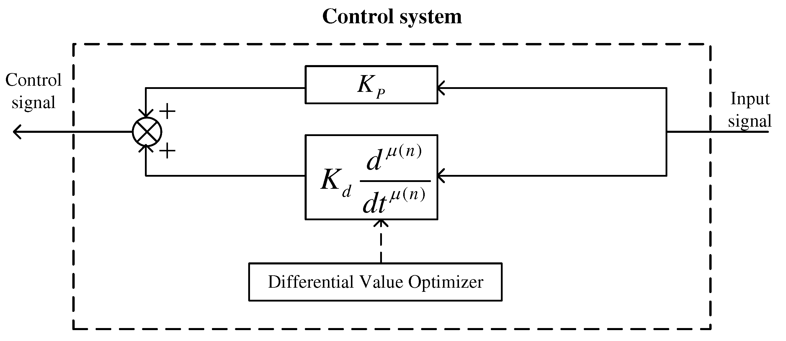
Figure 2 illustrates the IFOPD control system under centralized control mode. For simplicity, a P controller under centralized control mode will be referred to as CP in the follow-up.

3.2. An Improved Decentralized Control Strategy

The control system consists of a controller (electronic unit) and an actuator. The controller needs to detect continuously whether an earthquake has occurred or not, but the long idle state may cause the controller to fail in the presence of some sudden event. From Figure 2, we verify that, when the controller fails, the system enters in an uncontrolled state and, therefore, potential safety issues emerge. Decentralized control is usually employed to increase the reliability of the control system. A decentralized architecture divides the control system into different subsystems. Each subsystem consists of a controller (that outputs multiple control signals) and several actuators. When some controllers fail, the remaining systems are able to guarantee that the control system still has some relevant output action.

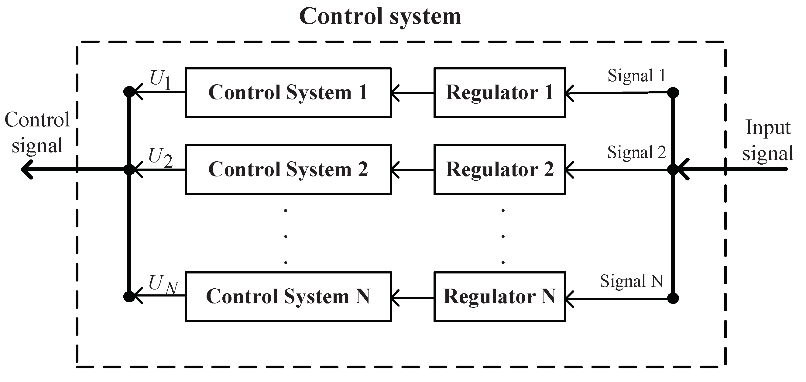
Herein, to improve the performance of the traditional decentralized strategy, a regulator is introduced into the control architecture. The regulator is a controllable scale factor that can adjust the amplitude of the feedback signal. Figure 3 depicts the structure of the proposed decentralized controller.

The control action of each controller in the control system can be calculated by the following equation:

$$\begin{array}{c}\hfill U_i\left(k\right)=K_{pi}{F}_i\left(k\right)+\sum _{j=0}^{M_1-1}{K}_{di}{h}^{-{\mu }_i\left(k\right)}{q}_j{F}_i(k-j)+\sum _{j=M_1}^{k-1}{K}_{di}{h}^{-{\mu }_i\left(k\right)}{q}_{M_1}{F}_i(k-j),k>M_1,i\in [1,N],\end{array}$$

(7)

where $F_i\left(k\right)=R_{i}f\left(k\right)$ and $R_i$ is a constant representing the scaling factor of the regulator. As before, the symbol $f\left(k\right)$ represents the displacement feedback signal, consisting of the displacement of the floor with the largest vibration in the subsystem.

For decentralized systems with regulators, the controller output is the result of the synergies between the various subsystems. However, when one particular subsystem fails, the parameters of the other control subsystems may not be optimal. To solve this problem, a fault self-regulation strategy is proposed, where all faults are analyzed beforehand, and the optimal parameters (for all faults) are calculated and stored. When a fault is detected, the parameters of the control system are updated according to the current detected fault.

Under an earthquake excitation, the implementation process of the fault self-regulation strategy is as follows:

• Step 1: Check if there is a fault in the control subsystem. If “yes”, jump to step 2; otherwise, if “no”, jump to step 3;
• Step 2: Update the control system parameters according to the fault situation;
• Step 3: Run the control system and output the corresponding control actions.

In the follow-up, a P-type controller, either under decentralized control with regulators and self-regulation, or under traditional decentralized control, is referred as DRP or DP, respectively.

4. Simulation Analysis

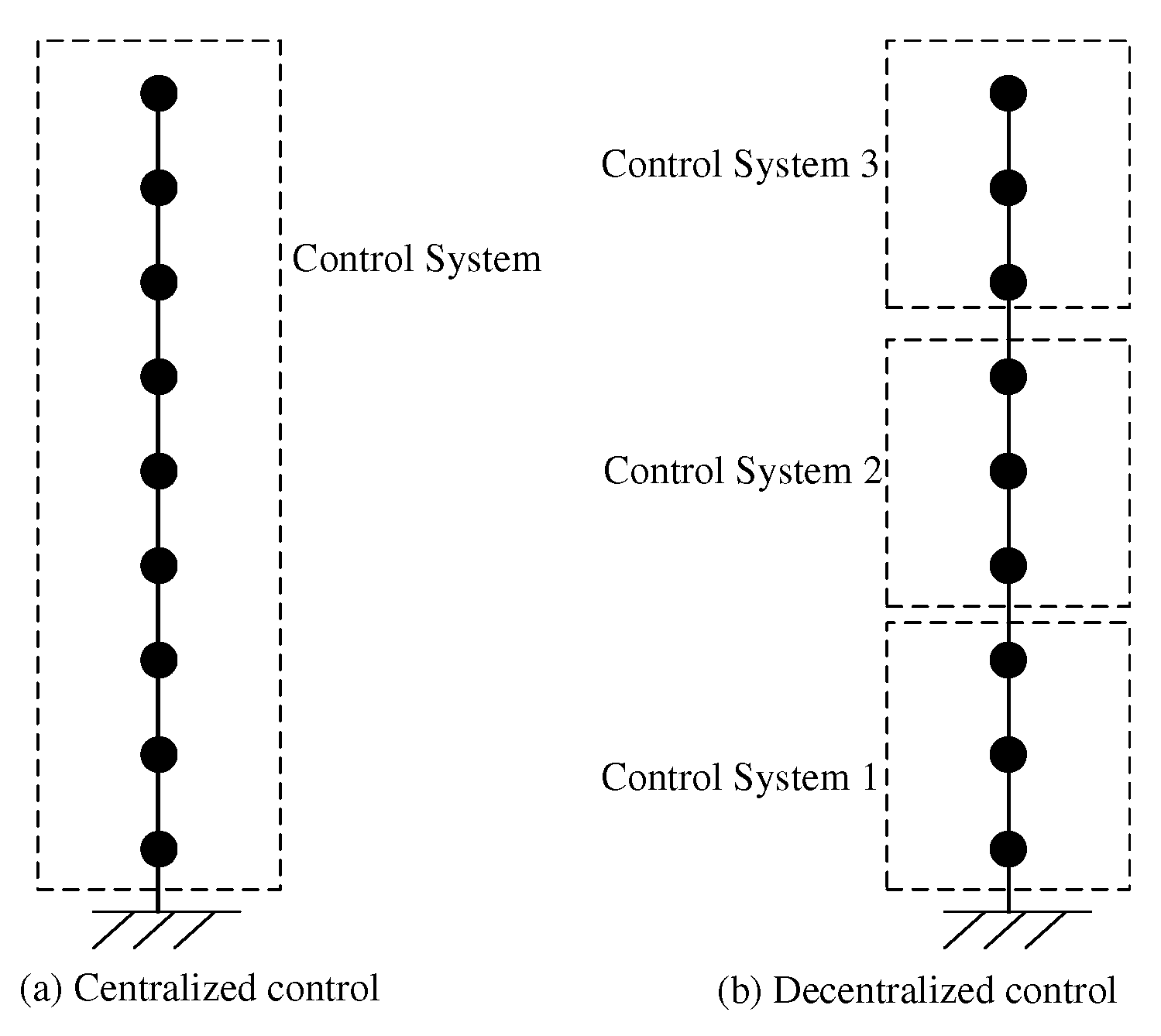
We consider a 9-floor building structure with the parameters shown in

Table A1. Structural parameters of 9-floor buildings.

Floor	1	2	3	4	5	6	7	8	9
Height (m)	4	3.3	3.3	3.3	3.3	3.3	3.3	3.3	3.3
Quality (kg)	29890	21700	21700	21700	21700	21700	21700	21700	21700
Rigidity ($1\times {10}^7$ N/m)	1.764	2.08	2.08	2.08	2.08	2.08	2.08	2.08	2.08

. The excitation signal is the El-centro seismic wave. Figure 4 depicts a diagram of the control system. When the centralized strategy is adopted, the input signal of the control system is the displacement of the 9th floor. Alternatively, when the decentralized control strategy is used, the input signals of the control subsystems 1, 2, and 3 are the displacements of the 3rd, 6th, and 9th floors, respectively.

When the control system is fault-free, the maximum displacement of the building structure is at the top floor, and the fitness function $g_1$ given in the formula (8) is selected to optimize the parameters by means of a PSO algorithm:

$$\begin{array}{c}\hfill g_1=\overline{g_{19}},g_{19}\left(j\right)=\left\{\begin{array}{cc}{X}_{19}\left(j\right),\hfill & X_{19}\left(j\right)\le X_{max}\hfill \\ {\omega }_1{X}_{19}\left(j\right),\hfill & X_{19}\left(j\right)>X_{max}\hfill \end{array}\right.,j=1,2\cdots jmax.\end{array}$$

(8)

When the control system fails, the floor with the largest displacement may be, or may be not, the top floor. In this case, the fitness function $g_2$ is selected, given by:

$$\begin{array}{c}\hfill g_2=\overline{g_{23}}+\overline{g_{26}}+\overline{g_{29}},g_{2i}\left(j\right)=\left\{\begin{array}{cc}{X}_{2i}\left(j\right),\hfill & X_{2i}\left(j\right)\le X_{max}\hfill \\ {\omega }_1{X}_{2i}\left(j\right),\hfill & X_{2i}\left(j\right)>X_{max}\hfill \end{array}\right.,i=3,6,9,j=1,2,\cdots ,jmax,\end{array}$$

(9)

where the symbols $\overline{g_{1i}}$ and $\overline{g_{2i}}$ represent the average displacement of the floor i, $g_{1i}\left(j\right)$ and $g_{2i}\left(j\right)$ stand for the displacement of floor i at the j-th time, $X_{max}$ is the maximum selected displacement, and ${\omega }_1=100$.

In the following experiments, the El-centro seismic wave is used as the excitation signal. An offline PSO optimization algorithm is used to optimize the control parameters $K_p$, $K_d$, $\mu$ and R. The fitness function $g_1$ is adopted in the optimization of the control parameters in the absence of any failure. On the other hand, the fitness function $g_2$ is used for the case when the controller fails. The configuration of the PSO used in this paper is shown in

Table A2. PSO optimization algorithm configuration.

Name of Parameters	Value of Parameters
Particle number	50
Number of Iterations/Number of repeated experiments	300/50
Scaling factors	$C_1=C_2=2$, $w=0.6$, $V_{max}=1$, $V_{min}=-1$
Parameter optimization range	$k_p\in [0,20]$, $k_i\in [0,5]$, $u,R\in [0,2]$

, and the values of the parameters obtained through optimization are listed in

Table A3. Control system parameters.

Name of Control System	Control System Parameter Value
CPD	$[K_p,K_d]=[0.01,3.997]$
CFOPD	$[K_p,K_d,\mu ]=[20,5,1.63]$
CIFOPD	$[K_p,K_d,\mu ]=[15.614,2.996,\sim ]$
DRPD	$[K_{p1},K_{d1},K_{p2},K_{d2},K_{p3},K_{d3},R_1,R_2,R_3]$
	$=[20,4.91,19.88,5,20,5,1.985,2,2]$
DRFOPD	$[K_{p1},K_{d1},{\mu }_1,K_{p2},K_{d2},{\mu }_2,K_{p3},K_{d3},{\mu }_3,R_1,R_2,R_3]$
	$=[10.19,5,1.198,0.0976,5,1.627,20,5,1.228,0.7781,1.1273,2]$
DRIFOPD	$[K_{p1},K_{d1},{\mu }_1,K_{p2},K_{d2},{\mu }_2,K_{p3},K_{d3},{\mu }_3,R_1,R_2,R_3]$
	$=[19.65,3.881,\sim ,2.821,4.046,\sim ,10.06,2.501,\sim ,0.8483,1.719,1.842]$
Fault case 1: DIFOPD	$[K_{p1},K_{d1},{\mu }_1,K_{p2},K_{d2},{\mu }_2,K_{p3},K_{d3},{\mu }_3]$
	$=[20,4.8086,\sim ,\times ,\times ,\times ,15.2195,3.3904,\sim ]$
Fault case 1: DRIFOPD	$[K_{p1},K_{d1},{\mu }_1,K_{p2},K_{d2},{\mu }_2,K_{p3},K_{d3},{\mu }_3,R_1,R_2,R_3]$
	$=[20,2.9654,\sim ,\times ,\times ,\times ,19.587,3.0118,\sim ,0.5672,\times ,1.5528]$
Fault case 2: DIFOPD	$[K_{p1},K_{d1},{\mu }_1,K_{p2},K_{d2},{\mu }_2,K_{p3},K_{d3},{\mu }_3]$
	$=[\times ,\times ,\times ,16.7368,5,\sim ,\times ,\times ,\times ]$
Fault case 2: DRIFOPD	$[K_{p1},K_{d1},{\mu }_1,K_{p2},K_{d2},{\mu }_2,K_{p3},K_{d3},{\mu }_3,R_1,R_2,R_3]$
	$=[\times ,\times ,\times ,6.8145,3.56,\sim ,\times ,\times ,\times ,\times ,1.7177,\times ]$
Fault case 3: DIFOPD	$[K_{p1},K_{d1},{\mu }_1,K_{p2},K_{d2},{\mu }_2,K_{p3},K_{d3},{\mu }_3]$
	$=[20,4.8086,\sim ,\times ,\times ,\times ,\times ,\times ,\times ]$
Fault case 3: DRIFOPD	$[K_{p1},K_{d1},{\mu }_1,K_{p2},K_{d2},{\mu }_2,K_{p3},K_{d3},{\mu }_3,R_1,R_2,R_3]$
	$=[0.01,4.9266,\sim ,\times ,\times ,\times ,\times ,\times ,\times ,1.0702,\times ,\times ]$

Note: the symbol ∼ means that the value changes with time, and the symbol × refers to the fault of the controller.

.

4.1. Analysis of the Centralized Control

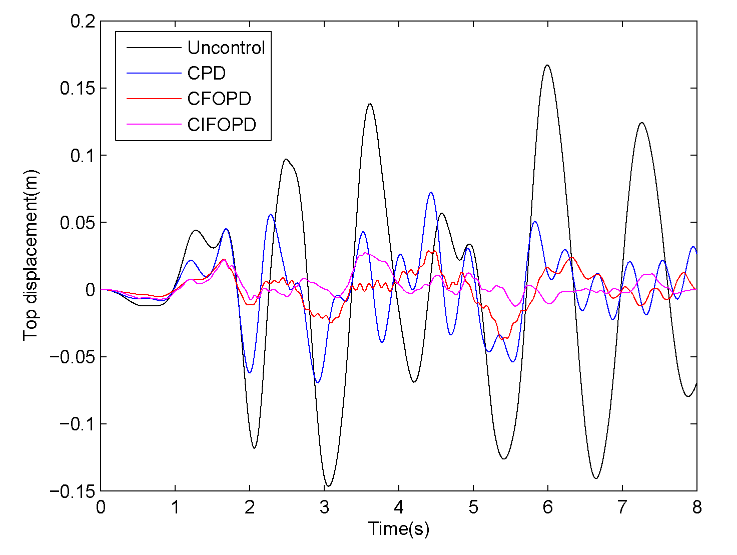
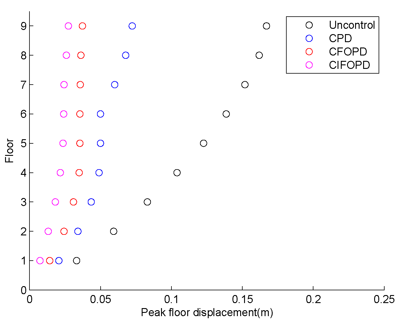
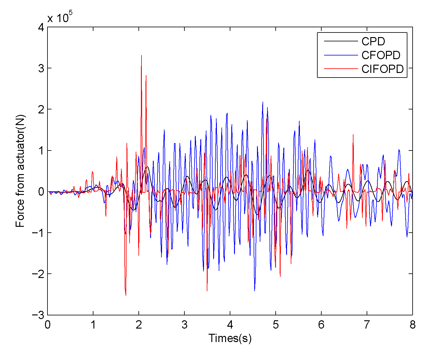
The displacement of the 9-floor building under centralized control is shown in Figure 5 and Figure 6. We verify that the CFOPD and CIFOPD yield acceptable performance, while the CPD leads to poor results. The maximum displacement obtained with the CFOPD is 0.0373 m and the average displacement given by (6) is $g_1=0.0096$ m. For the CIFOPD, the maximum displacement is 0.0274 m and the average displacement is $g_1=0.0057$ m. Therefore, the maximum displacement for the CIFOPD, when compared to the CFOPD, is reduced by 36.1% and the average displacement $g_1$ is reduced by 68.4%. The control signals of the CPD, CFOPID, and CIFOPID are shown in Figure 7. It follows that the CIFOPD is superior to the CFOPD.

4.2. Analysis of the Decentralized Control

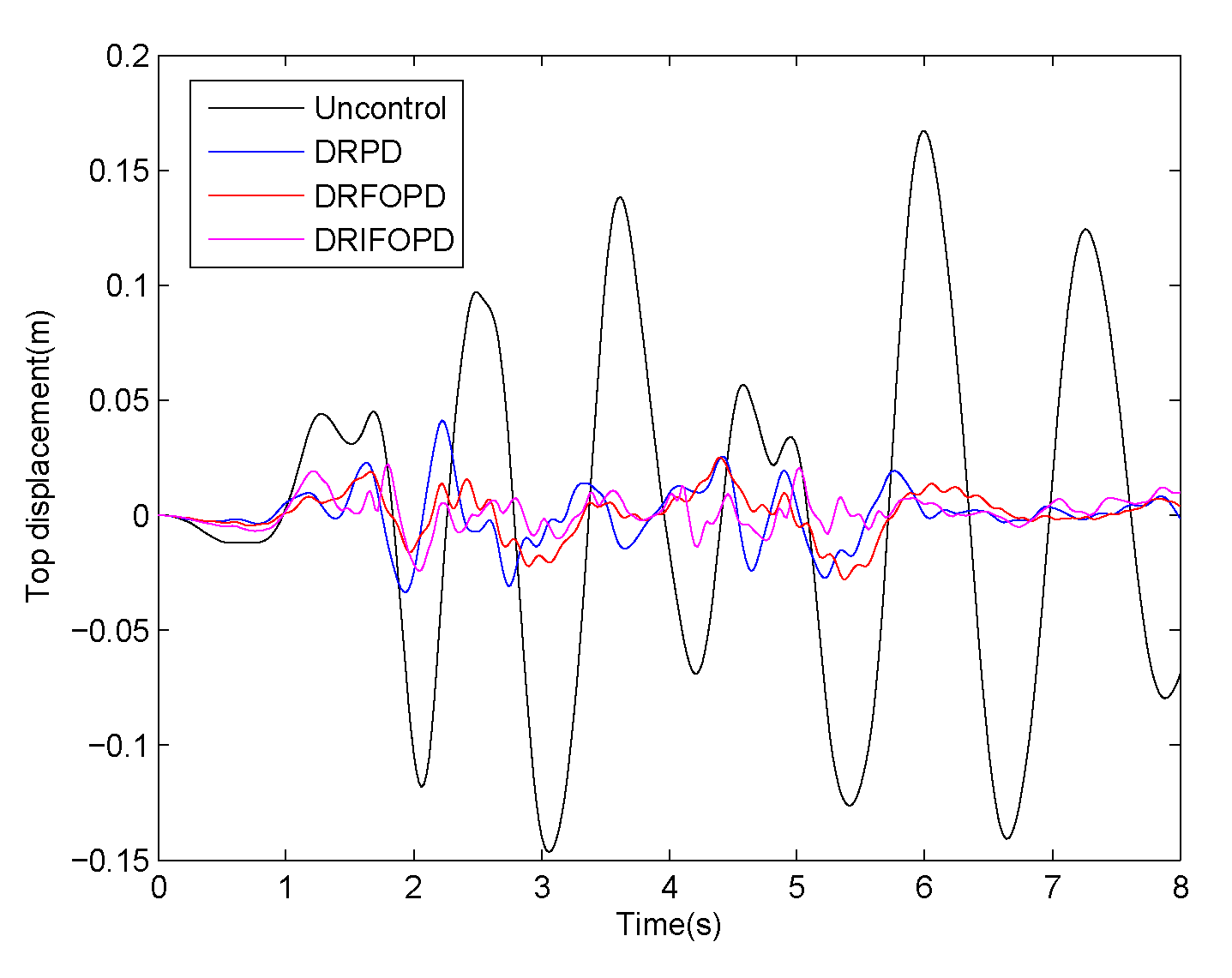
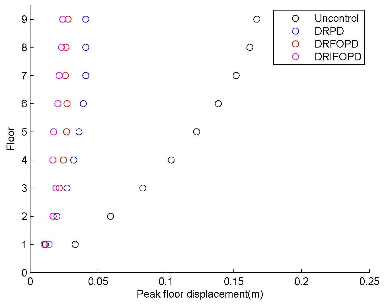
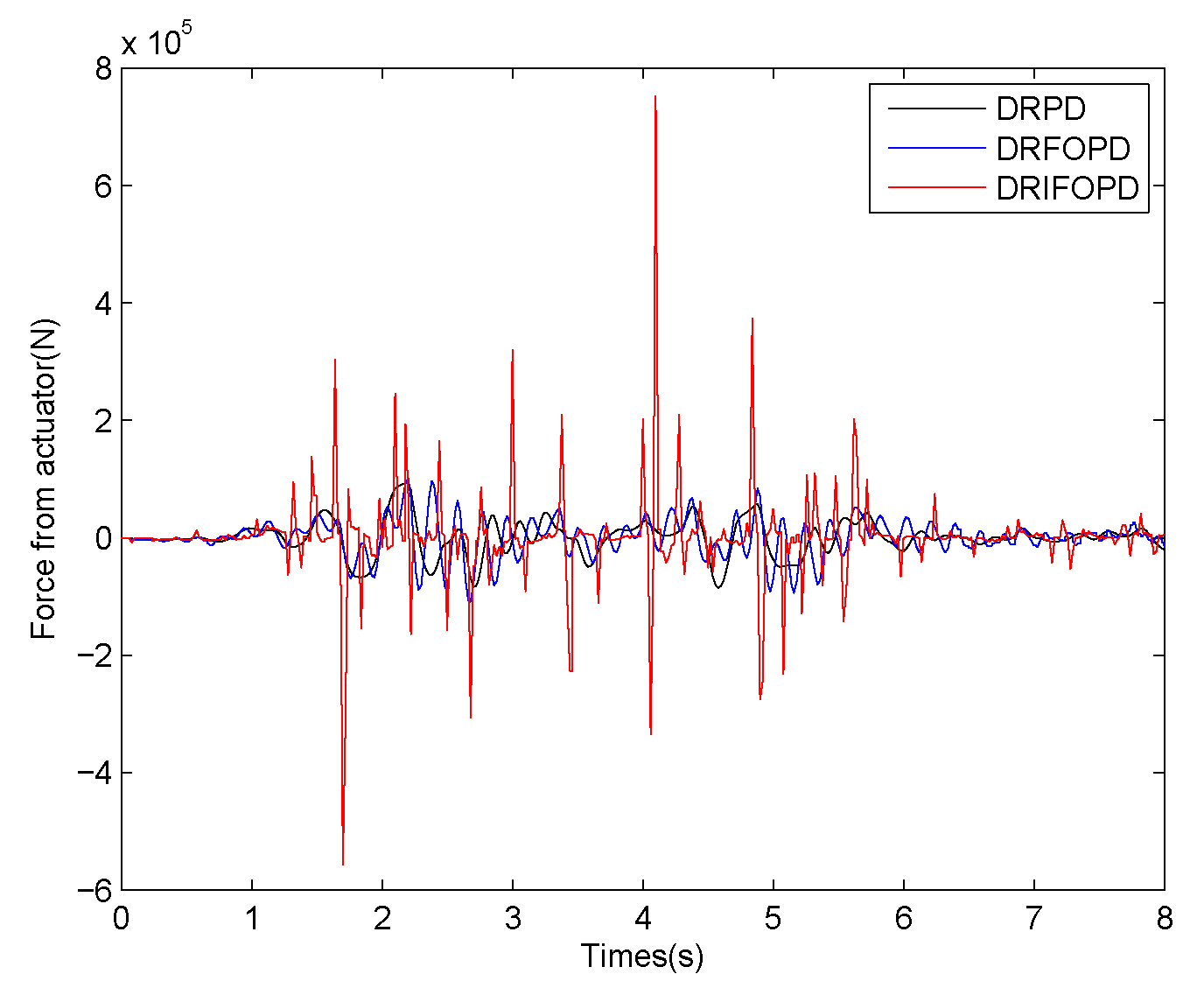
Figure 8 and Figure 9 depict the displacement of the 9-floor building structure under decentralized control. The maximum displacement obtained with the DRFOPD is 0.0279 m and the average displacement is $g_1=0.0068$ m. The maximum displacement for the DRIFOPD is 0.024 m and the average displacement is $g_1=0.0054$ m. Comparing both controllers, we verify that the maximum displacement obtained with the DRIFOPD is reduced by 16.3%, and the average displacement $g_1$ is reduced by 20.6%. The control signals of the DRPD, DRFOPD, and DRIFOPD are shown in Figure 10. We observe that the DRIFOPD is better than the DRFOPD.

In conclusion, we verify that the maximum and average displacements obtained with the improved decentralized control are smaller than those yielded by the centralized control strategy. At the same time, the comparative analysis shows that the DRIFOPD has the best performance.

4.3. Fault Analysis

In this subsection, we analyze the control performance and reliability of the DRIFOPD in the presence of one fault. Three scenarios are tested: fault case 1—the control subsystem 2 fails; fault case 2—both the control subsystems 1 and 3 fail; fault case 3—both the control subsystems 2 and 3 fail.

4.3.1. Fault Case 1

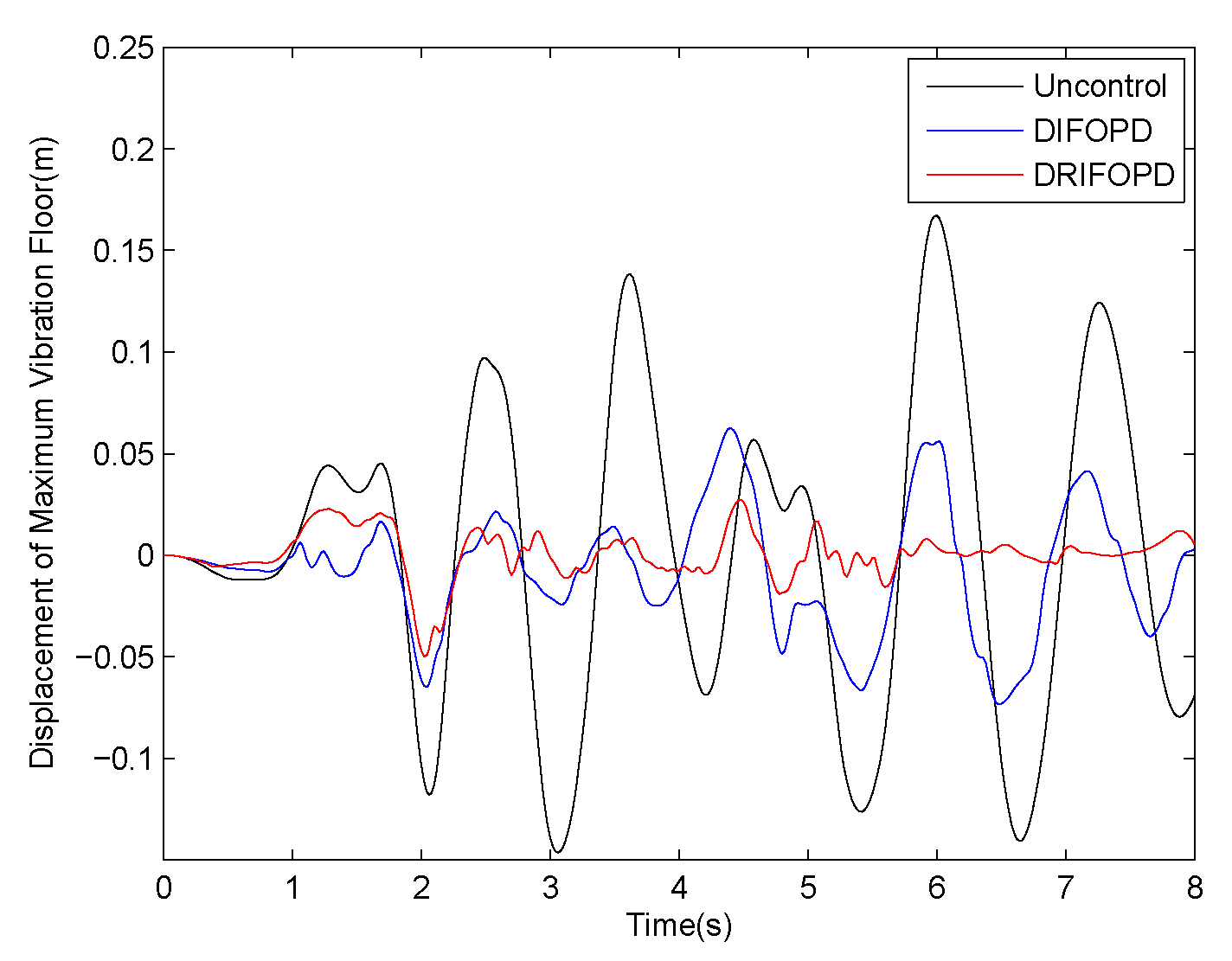
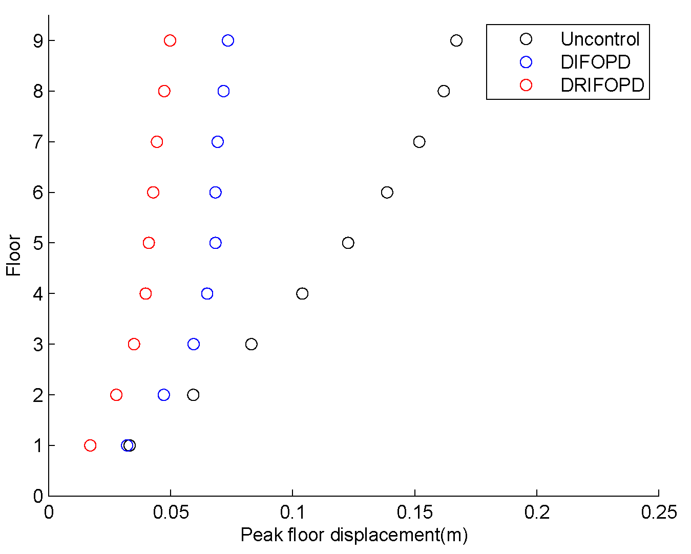
For the fault case 1, both the DIFOPD and DRIFOPD controllers have acceptable performance after the fault. Figure 11 and Figure 12 depict the displacements of the structure. We verify that the maximum and average displacements $g_2$ obtained with the DRIFOPD are much smaller than those obtained with the DIFOPD. This result indicates that the performance of the DRIFOPD is better than the one exhibited by the DIFOPD.

4.3.2. Fault Case 2

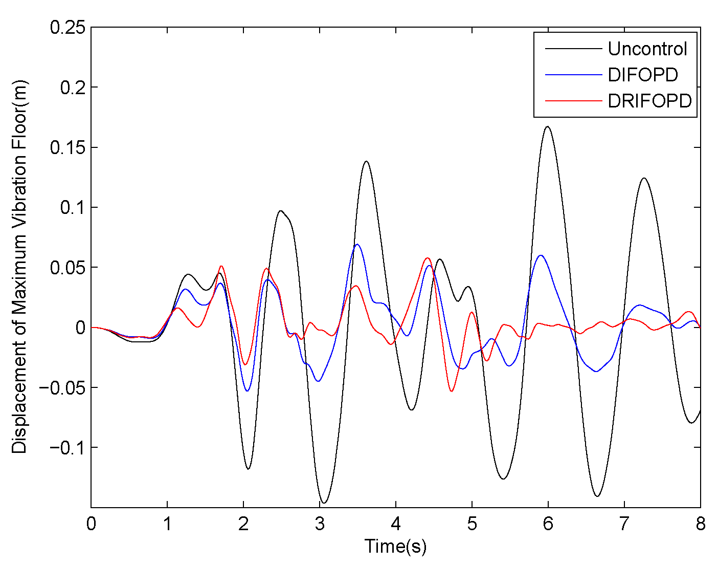
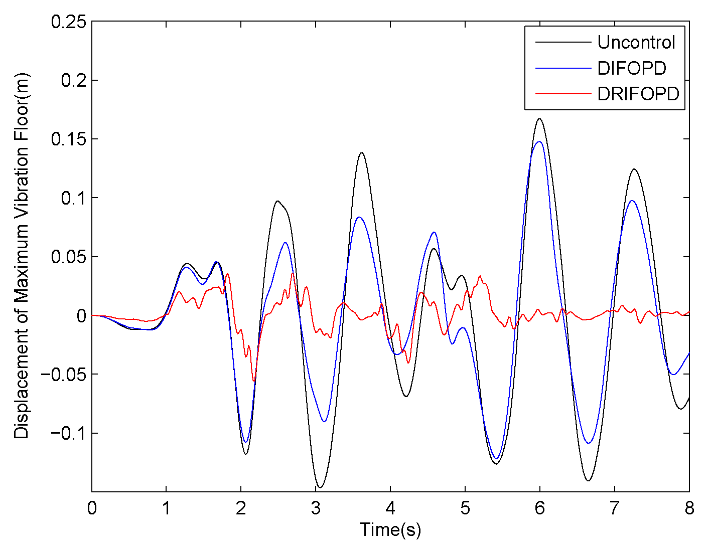
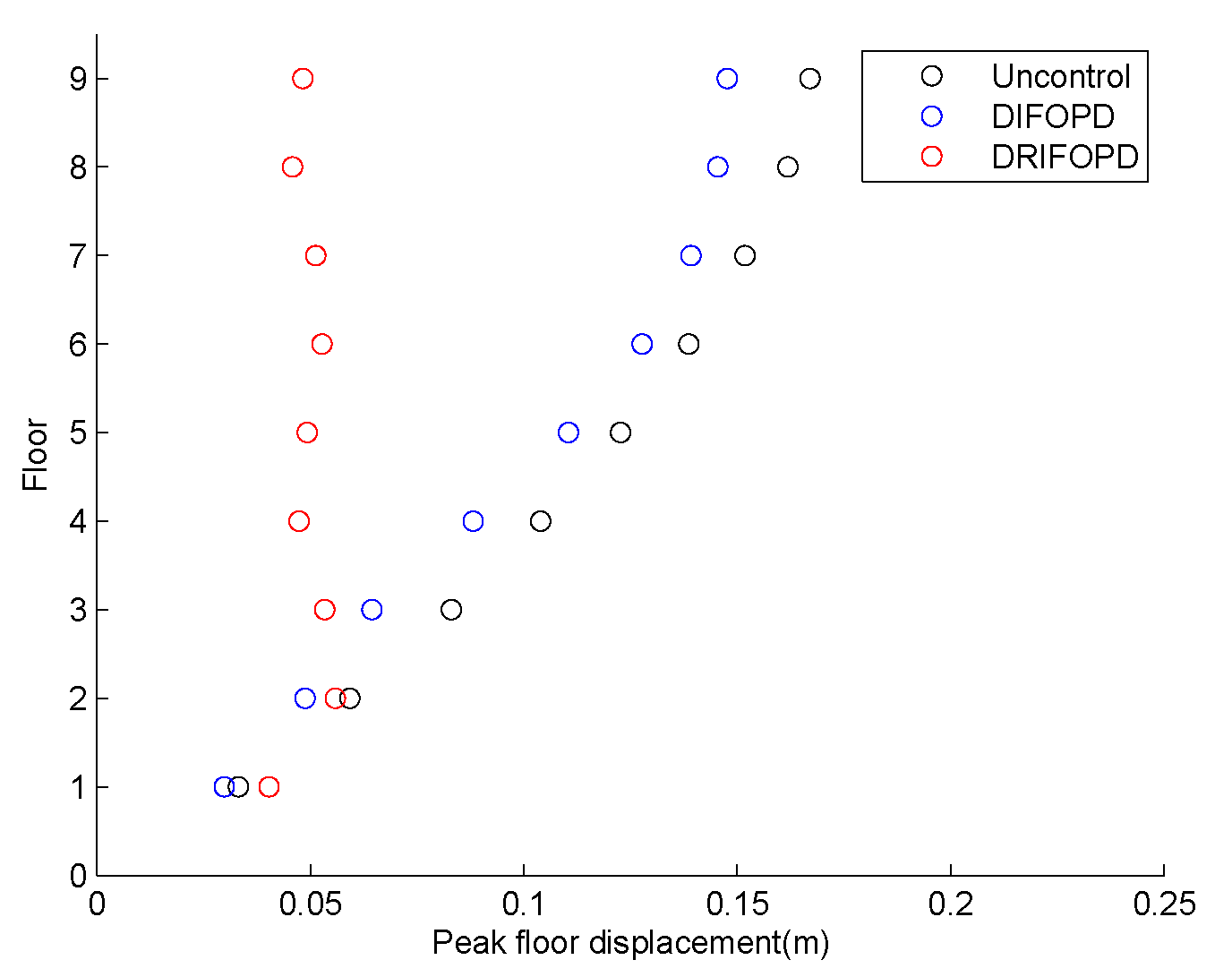
For the fault case 2, the displacement of the 9-floor building structure is shown in Figure 13 and Figure 14. The maximum displacement for the DIFOPD is 0.0691 m and the average displacement is $g_2=0.0438$ m. The maximum displacement for the DRIFOPD is 0.0579 m and the average displacement is $g_2=0.009$ m. Compared with the DIFOPD, the maximum displacement for the DRIFOPD is reduced by 16.2%, and the average displacement $g_2$ is reduced by 79.4%. The results show that (i) both the DIFOPD and the DRIFOPD have some control action under fault case 2, and (ii) the DRIFOPD is better than the DIFOPD.

4.3.3. Fault Case 3

For the fault case 3, the displacement of the 9-floor building structure is shown in Figure 15 and Figure 16. Comparing the displacement obtained with the DIFOPD with the one for the uncontrolled mode, we conclude that the DIFOPD has almost a complete failure. This result occurs because, in the decentralized strategy, the control actions of subsystems are different. The control subsystem 1 of the DIFOPD produces outputs with very small amplitudes that mainly play a regulating role. Therefore, when the control subsystems 2 and 3 fail, the vibration of the building structure can not be suppressed merely by the control subsystem 1. However, when the DIFOPD fails, the DRIFOPD still has a good control effect. In fact, when the self-tuning strategy in the DRIFOPD detects the fault, it makes the output of the control subsystem 1 more significant by adjusting the parameters, so as to maintain the control performance of the global system. The results show that the performance of the DRIFOPD is better than that of the DIFOPD in fault case 3. Moreover, the results also prove that the reliability of the DRIFOPD is better than that of the DIFOPD.

5. Conclusions

The paper addressed the design of a composite control system to improve the performance and reliability of building structure vibration control. An improved FOPD controller was proposed. Simulations under centralized control revealed that the performance of the CIFOPD is much better than the one exhibited by the CFOPD. A decentralized strategy was then designed by adding a regulator and fault self-regulation to a traditional decentralized controller. The combination of the IFOPD with the improved decentralized strategy led to the DRIFOPD controller. Simulation results verified that the DRIFOPD has a superior reliability and excellent control performance.

References

- Rahimi, Z.; Sumelka, W.; Ahmadi, S.R.; Baleanu, D. Study and control of thermoelastic damping of in-plane vibration of the functionally graded nano-plate. J. Vib. Control. 2019, 25, 2850–2862. [Google Scholar] [CrossRef]
- Jajarmi, A.; Hajipour, M.; Sajjadi, S.S.; Baleanu, D. A robust and accurate disturbance damping control design for nonlinear dynamical systems. Optim. Control. Appl. Methods 2019, 40, 375–393. [Google Scholar] [CrossRef]
- Chuang, C.H.; Wu, D.N.; Wang, Q. LQR for state-bounded structural control. J. Dyn. Syst. Meas. Control. 1996, 118, 113–119. [Google Scholar] [CrossRef]
- Soleymani, M.; Abolmasoumi, A.H.; Bahrami, H.; Khalatbari-S, A.; Khoshbin, E.; Sayahi, S. Modified sliding mode control of a seismic active mass damper system considering model uncertainties and input time delay. J. Vib. Control. 2018, 24, 1051–1064. [Google Scholar] [CrossRef]
- Zizouni, K.; Fali, L.; Sadek, Y.; Bousserhane, I.K. Neural network control for earthquake structural vibration reduction using MRD. Front. Struct. Civ. Eng. 2019, 13, 1171–1182. [Google Scholar] [CrossRef]
- Maruani, J.; Bruant, I.; Pablo, F.; Gallimard, L. Active vibration control of a smart functionally graded piezoelectric material plate using an adaptive fuzzy controller strategy. J. Intell. Mater. Syst. Struct. 2019, 30, 2065–2078. [Google Scholar] [CrossRef]
- Wang, J.; Chen, W.; Chen, Z.; Huang, Y.; Huang, X.; Wu, W.; He, B.; Zhang, C. Neural Terminal Sliding-Mode Control for Uncertain Systems with Building Structure Vibration. Complexity 2019, 2019, 1507051. [Google Scholar] [CrossRef]
- Zhang, X.Y.; Zhang, S.Q.; Wang, Z.X.; Qin, X.S.; Wang, R.X.; Schmidt, R. Disturbance rejection control with H∞ optimized observer for vibration suppression of piezoelectric smart structures. Mech. Ind. 2019, 20, 202. [Google Scholar] [CrossRef]
- Thenozhi, S.; Yu, W. Stability analysis of active vibration control of building structures using PD/PID control. Eng. Struct. 2014, 81, 208–218. [Google Scholar] [CrossRef]
- Guclu, R.; Yazici, H. Vibration control of a structure with ATMD against earthquake using fuzzy logic controllers. J. Sound Vib. 2008, 318, 36–49. [Google Scholar] [CrossRef]
- Etedali, S.; Zamani, A.A.; Tavakoli, S. A GBMO-based PIλDμ controller for vibration mitigation of seismic-excited structures. Autom. Constr. 2018, 87, 1–12. [Google Scholar] [CrossRef]
- Coronel-Escamilla, A.; Torres, F.; Gómez-Aguilar, J.; Escobar-Jiménez, R.; Guerrero-Ramírez, G. On the trajectory tracking control for an SCARA robot manipulator in a fractional model driven by induction motors with PSO tuning. Multibody Syst. Dyn. 2018, 43, 257–277. [Google Scholar] [CrossRef]
- Zhong, J.; Li, L. Fractional-order system identification and proportional-derivative control of a solid-core magnetic bearing. ISA Trans. 2014, 53, 1232–1242. [Google Scholar] [CrossRef] [PubMed]
- Silva, M.F.; Machado, J.T.; Lopes, A. Fractional order control of a hexapod robot. Nonlinear Dyn. 2004, 38, 417–433. [Google Scholar] [CrossRef]
- Zamani, A.A.; Tavakoli, S.; Etedali, S. Fractional order PID control design for semi-active control of smart base-isolated structures: A multi-objective cuckoo search approach. ISA Trans. 2017, 67, 222–232. [Google Scholar] [CrossRef] [PubMed]
- Petráš, I.; Vinagre, B. Practical application of digital fractional-order controller to temperature control. Acta Montan. Slovaca 2002, 7, 131–137. [Google Scholar]
- Delavari, H.; Ranjbar, A.; Ghaderi, R.; Momani, S. Fractional order control of a coupled tank. Nonlinear Dyn. 2010, 61, 383–397. [Google Scholar] [CrossRef]
- Chen, L.; Wu, R.; He, Y.; Yin, L. Robust stability and stabilization of fractional-order linear systems with polytopic uncertainties. Appl. Math. Comput. 2015, 257, 274–284. [Google Scholar] [CrossRef]
- Chen, L.; Cao, J.; Wu, R.; Machado, J.T.; Lopes, A.M.; Yang, H. Stability and synchronization of fractional-order memristive neural networks with multiple delays. Neural Netw. 2017, 94, 76–85. [Google Scholar] [CrossRef]
- Raji, R.; Hadidi, A.; Ghaffarzadeh, H.; Safari, A. Robust decentralized control of structures using the LMI H-infinity controller with uncertainties. Smart Struct. Syst. 2018, 22, 547–560. [Google Scholar]
- Lei, Y.; Wu, D.; Liu, L. A decentralized structural control algorithm with application to the benchmark control problem for seismically excited buildings. Struct. Control. Health Monit. 2013, 20, 1211–1225. [Google Scholar] [CrossRef]
- Linderman, L.E.; Spencer Jr, B. Decentralized active control of multistory civil structure with wireless smart sensor nodes. J. Eng. Mech. 2016, 142, 04016078. [Google Scholar] [CrossRef]
- Baghani, O. Solving state feedback control of fractional linear quadratic regulator systems using triangular functions. Commun. Nonlinear Sci. Numer. Simul. 2019, 73, 319–337. [Google Scholar] [CrossRef]
- Chen, Y.Q.; Moore, K.L. Discretization schemes for fractional-order differentiators and integrators. IEEE Trans. Circuits Syst. Fundam. Theory Appl. 2002, 49, 363–367. [Google Scholar] [CrossRef]
- Zhenbin, W.; Zhenlei, W.; Guangyi, C.; Xinjian, Z. Digital implementation of fractional order PID controller and its application. J. Syst. Eng. Electron. 2005, 16, 116–122. [Google Scholar]
- Hall, J.F. Problems encountered from the use (or misuse) of Rayleigh damping. Earthq. Eng. Struct. Dyn. 2006, 35, 525–545. [Google Scholar] [CrossRef]
- Del Valle, Y.; Venayagamoorthy, G.K.; Mohagheghi, S.; Hernandez, J.C.; Harley, R.G. Particle swarm optimization: Basic concepts, variants and applications in power systems. IEEE Trans. Evol. Comput. 2008, 12, 171–195. [Google Scholar] [CrossRef]
- Kulkarni, R.V.; Venayagamoorthy, G.K. Particle swarm optimization in wireless-sensor networks: A brief survey. IEEE Trans. Syst. Man, Cybern. Part C (Appl. Rev.) 2010, 41, 262–267. [Google Scholar] [CrossRef] [Green Version]
Figure 1.
Schematic diagram of a vibration control system of a building structure.
Figure 2.
Control system using the IFOPD under a centralized control mode.
Figure 3.
Decentralized control system with a regulator.
Figure 4.
Schematic diagram of the control system of a 9-floor building structure.
Figure 5.
Top displacement curve under centralized control.
Figure 6.
Maximum displacement of each floor under centralized control.
Figure 7.
Forces output generated by the actuators under the action of the CPD, CFOPID, and CIFOPID controllers.
Figure 8.
Top displacement curve under decentralized control.
Figure 9.
Maximum displacement of each floor under decentralized control.
Figure 10.
Forces output generated by the actuators under the action of the DRPD, DRFOPD, and DRIFOPD controllers.
Figure 11.
The displacement of the maximum vibration floor under fault case 1.
Figure 12.
Maximum displacement of each floor under fault case 1.
Figure 13.
The displacement of the maximum vibration floor under fault case 2.
Figure 14.
Maximum displacement of each floor under fault case 2.
Figure 15.
The displacement of the maximum vibration floor under fault case 3.
Figure 16.
Maximum displacement of each floor under fault case 3.
© 2020 by the authors. Licensee MDPI, Basel, Switzerland. This article is an open access article distributed under the terms and conditions of the Creative Commons Attribution (CC BY) license (http://creativecommons.org/licenses/by/4.0/).
Share and Cite
MDPI and ACS Style
Xu, K.; Chen, L.; Wang, M.; Lopes, A.M.; Tenreiro Machado, J.A.; Zhai, H. Improved Decentralized Fractional PD Control of Structure Vibrations. Mathematics 2020, 8, 326. https://doi.org/10.3390/math8030326
AMA Style
Xu K, Chen L, Wang M, Lopes AM, Tenreiro Machado JA, Zhai H. Improved Decentralized Fractional PD Control of Structure Vibrations. Mathematics. 2020; 8(3):326. https://doi.org/10.3390/math8030326
Chicago/Turabian StyleXu, Kang, Liping Chen, Minwu Wang, António M. Lopes, J. A. Tenreiro Machado, and Houzhen Zhai. 2020. "Improved Decentralized Fractional PD Control of Structure Vibrations" Mathematics 8, no. 3: 326. https://doi.org/10.3390/math8030326
Note that from the first issue of 2016, this journal uses article numbers instead of page numbers. See further details here.