A Multi-Criteria Decision Support Framework for Inland Nuclear Power Plant Site Selection under Z-Information: A Case Study in Hunan Province of China

Abstract

To promote the development of nuclear power project in inland China, a specialized multi-criteria decision support framework is constructed for the site selection of inland nuclear power plants in this work. The best worst method (BWM), decision-making trial and evaluation laboratory (DEMATEL), and technique for order performance by similarity to ideal solution (TOPSIS) are integrated with Z-numbers, namely Z-BWM, Z-DEMATEL, and Z-TOPSIS. Z-BWM and Z-DEMATEL are combined to produce the weights of criteria, and an extended Z-TOPSIS is utilized to determine the ranking of all alternatives. Finally, a case study is performed in Hunan province to demonstrate the practicability of the proposed decision support framework. The robustness and feasibility of the proposed method are shown by an in-depth analysis of the decision results.

1. Introduction

Faced with the increasingly serious problem of environmental pollution and carbon dioxide emission, nuclear power has become a low-carbon alternative energy source that could transform the global energy structure [1]. The International Energy Agency (IAEA) forecasted that until 2050, the global potential of nuclear power remains high and will mainly lie in Asia, especially in China. The nuclear power industry in China began in 1955 with the establishment of China National Nuclear Corporation (CNNC). As of October 2019, China ranks third in the world in terms of total nuclear power electricity generation, accounting for about one-tenth of global nuclear power being generated. The mainland China has 48 nuclear reactors with a capacity of 45.5 GW, 9 under construction with a capacity of 8.3 GW, and more being about to start construction.

Nuclear energy is generated by the splitting of atoms inside uranium, as a relatively clean non-fossil energy, it produces more electricity or heat per unit than fossil fuels, with less of environmental impact [2]. Some countries, such as France and Slovak Republic, have been meeting over 50% of the energy demand with nuclear energy, and many others like India and Korea are on their way. Although the reasons for expanding nuclear energy in a carbon-constrained future are strong, there are still some shackles in some countries because of a series of problems like policy changes, cost overruns, and long period of construction [3]. Therefore, it is urgent to develop a scientific and reasonable nuclear power plant (NPP) site selection plan, so as to improve the operation safety of NPPs and reduce the construction cost. Now, there are more than 400 nuclear plants in the world, about half of which are in inland areas that are not prone to tsunamis or typhoons. China has a total of 48 nuclear power units in operation, but they are all in coastal areas. The specific research on the site selection of China’s inland NPPs is still insufficient. In this work, a multi-criteria decision support framework is provided to identify the best site for inland NPPs in China, and the contributions are summarized as follows:

(1) The existing researches on multi-criteria decision-making (MCDM) problems inevitably involve the uncertainly and unreliability of human preferences. Therefore, Z-number is introduced into the proposed MCDM framework in this work, and all evaluation information is given using Z-number linguistic variables.

(2) Best worst method (BWM) and decision-making trial and evaluation laboratory (DEMATEL) are extended to Z-numbers, i.e., Z-BWM and Z-DEMATEL. The hybrid model not only considers the impact of the criterion relations on the criterion weights, but also provides a long-term improvement for inland NPP site selection.

(3) The technique for order performance by similarity to ideal solution (TOPSIS) is combined with Z-numbers, namely Z-TOPSIS. It can effectively reduce the influence of outliers, and provide more reliable ranking results than the classic TOPSIS.

(4) Currently, few researches focus on the site selection of China’s inland NPPs. Based on the reactor siting criteria developed by IAEA, a specialized evaluation system considering the eco-environment, geographic features, and socio-economic factors in China’s interior is constructed.

The structure of the paper is organized as follows. Section 2 reviews some studies related to NPP site selection. Section 3 introduces some basic concepts of Z-numbers. Section 4 presents the proposed framework for inland NPP site selection. Section 5 provides a case study in Hunan province of China. Section 6 conducts an in-depth analysis concerning selection results. Finally, Section 7 draws conclusions.

2. Literature Review

2.1. Methods for NPP Site Selection

In the recent literatures, many researches have been done for the site selection of NPPs, and most of them consider MCDM method as the most commonly used one [4]. For instance, Erdoğan and Kaya [5] applied the analytic hierarchy process (AHP) and TOPSIS determine the optimal site for NPPs in a fuzzy environment. Damoom et al. [6] proposed a geographical information system (GIS)-based multistage decision framework, which significantly contributes to the development in selecting specific sites for NPP installation in Saudi Arab. Based on the site selection guidelines of NPPs, Wang et al. [7] solved a location selection problem for a nuclear power plant construction in Vietnam by using a hybrid fuzzy analytic network process (ANP) and TOPSIS.

Although these innovative studies have made great contribution to NPP site selection, there are still some improvements. In view of the existing studies, most methods for location problems are evaluated by crisp/fuzzy and partially reliable information, it is usually given in the light of experts’ experience [8,9]. However, the fact is that some experts may not provide objective and accurate evaluation values because of the limitations of their cognition. Several studies have shown that information is not completely reliable in many MCDM processes [10,11,12]. Especially in the problem with complex information source and subjective evaluation information, a large amount of incomplete reliable information exists [13]. Z-number is a new concept integrating both cognitive information and the reliability of information, produced by Zadeh in 2011 [14]. It is more capable of describing human knowledge and is widely applied in complex and imprecise information processing [15,16]. Therefore, Z-number is employed in this paper because it can cope with the inherent fuzziness and uncertainty in the chosen decision-making scenario.

There are numerous MCDM techniques, among which AHP, ANP, and BWM are commonly used to determine the criterion weights in the site selection process [17,18]. Compared with other classic MCDM methods (such as AHP/ANP), in most of the cases BWM ensures higher consistency of evaluation results and reduces the number of required pairwise comparisons [19]. Since only the best/worst criteria needs to be compared with others, it reduces the mounts of calculation to some extent. This approach is well-known for its simplicity and flexibility and has been widely used in the recent studies [20,21]. However, BWM is similar to AHP, although it helps to determine the criterion weights in a short period, it fails to analyze the intrinsic causality relationships of criteria. DEMATEL was originally proposed by Memorial Institute in Geneva Research Center [22], Unlike BWM, it is a comprehensive method for the compilation and analysis of structural models that contain causal relationships between complex indicator frameworks [23]. The original DEMATEL is also improved by some scholars so as to make it comply with their research questions. For example, Shahi et al. [24] determined an ideal NPP site by means of modified model of fuzzy DEMATEL and GIS in Bushehr, Iran. To furnish a deep insight into evaluation results, Nie et al. [25] analyzed the interrelationships among criteria in the context of water security sustainability evaluation. However, few studies have further explored the impact of interrelationships on criterion weights. Therefore, BWM and DEMATEL with Z-numbers, i.e., Z-BWM and Z-DEMATE, are integrated to reinforce the reliability of criterion weights, because they serve different functions in the site selection of inland NPPs.

In terms of the ranking of site alternatives can be dealt with using the extended Z-TOPSIS in this work. The basic concept and implementation steps of TOPSIS was first developed by Huang [26]. It finds the optimal solution by choosing the alternative that has the shortest distance from the positive ideal and the farthest distance from the negative ideal solution. As a basic ranking method, TOPSIS can make full use of evaluation information without further requirements for information independence [27]. This advantage makes it appropriate for experts who are technical in nuclear power industry, but not necessarily in the area of theoretical decision-making. Moreover, it is easy to integrate with other MCDM approaches (such as AHP/BWM) and provides reliable evaluation results, which has led to this technique being used in many site selection problems [28]. Since TOPSIS is a technique that relies heavily on the value of information, the reliability of information will directly affect the quality of ranking results [29]. This approach is further extended to Z-numbers in our study.

2.2. Evaluation Criteria for Inland NPP Site Selection

The site selection for inland NPPs is a complex issue that requires the comprehensive and careful analysis of numerous criteria. Many researches established indicator frameworks related to the NPP site selection from three dimensions: biological, physical, and socio-economic [24,30,31,32]. Some studies mainly took the environmental compatibility, technical feasibility, security, and economic rationality into account for assessing site sustainability [5,7]. In addition, the NPP construction is also regarded as a spatial problem and involves a large amount of geophysical data, such as geology, hydrology, weather, and so on. Therefore, Yaar et al. [33] determined a potential site for future NPPs in Israel based on the demographic, seismologic, and geologic criteria. Basu [34] reviewed and summarized the NPP siting evaluation process in three countries, and outlined the state-of-the-practice of site evaluation criteria for NPPs from the aspects of natural, public, and emergency management planning. In the latest study of Arab Atomic Energy Agency (AAEA), Salman [35] considered not only the main geological and natural characteristics, but also the population density and the area characteristics around the site of the nuclear plant.

On the basis of expert opinions and relevant literature, a location decision criteria system for inland NPP site selection is constructed in this paper. The evaluation indicator framework is divided into three main dimensions, i.e., eco-environment (U₁), physical geography (U₂), and socio-economics (U₃). Details of the inland NPP indicator framework are described in

Table 1. The indicator framework for inland nuclear power plant (NPP) site selection.

Criteria	Sub-criteria	Category	Reference
U1	Distance from vegetation area U11	B	[24,30,31]
	Distance from groundwater-rich area U12	B
	Distance from protected area U13	B
U2	Slope stability U21	B	[32,33,34,36,37]
	Elevation stability U22	B
	Soil erosion U23	C
	Flood disasters U24	C
	Seismic activity U25	C
	Cooling water availability U26	B
	The atmospheric dispersion U27	B
U3	Land-use costs U31	C	[2,5,7,35,38,39]
	Population density U32	C
	Distance from Road U33	C
	Distance from Airports U34	B
	Distance from power grid U35	C
	Distance from hazardous facilities U36	B

. B and C respectively represent benefit-type (the more the better) criteria and cost-type (the less the better) criteria.

3. Preliminaries

Definition 1

([40,41]) A fuzzy set $\tilde{A}$ is defined on a universe $X$ and could be presented as $\tilde{A}=\left\{(x,{\mu }_{\tilde{A}}(x))|x\in X\right\}$. ${\mu }_{\tilde{A}}(x):X\to [0,1]$ is the degree of membership of $x$ in $\tilde{A}$. The membership function of a triangular type of fuzzy number $\tilde{A}=(m,n,q)$ can be defined as follows.

$${\mu }_{\tilde{A}}(x)=\{\begin{array}{l}0,x<m\\ \frac{x-m}{n-m},m\le x<n\\ \frac{q-x}{1-n},n\le x<q\\ 0,x\ge q,\end{array}$$

(1)

where n is the grade of ${\mu }_{\tilde{A}}(x)$, and q and m represent the upper and lower limits.

Definition 2

([42]) A Z-number $Z=(A,B)$ is an ordered pair of regular fuzzy numbers. The first component $A$ is a restriction on the values, which represents the uncertain random variables of. The second component $B$ is a reliability measurement of the first component. Typically, $A$ and $B$ can be expressed in natural language, such as (poor, unlikely) and (good, likely) There are some rules for converting Z-numbers to regular fuzzy numbers. A typical one is reviewed as follows.

Definition 3

([43]) Given a Z-number $Z=(\tilde{A},\tilde{B})$, where $\left\{\tilde{A}=(x,{\mu }_{\tilde{A}}(x))|x\in [0,1]\right\}$ and $\left\{\tilde{B}=(x,{\mu }_{\tilde{B}}(x))|x\in [0,1]\right\}$ are triangular membership functions. The second component $B$ can be translated into a crisp number.

$$\alpha =\frac{{\displaystyle \int x{\mu }_{\tilde{B}}(x)dx}}{{\displaystyle \int {\mu }_{\tilde{B}}(x)dx}}.$$

(2)

After that, the weight of the second component should be added to the first component$\tilde{A}$. The weighting formula is shown as below.

$${\tilde{Z}}^{\alpha }=\left\{(x,{\mu }_{{\tilde{A}}^{\alpha }})|{\mu }_{{\tilde{A}}^{\alpha }}(x)=\alpha {\mu }_{\tilde{A}}(x),x\in [0,1]\right\}.$$

(3)

Then, the weighted Z-number${\tilde{Z}}^{\alpha }$can be converted into a regular fuzzy number as below.

$${\tilde{Z}}^{\prime }=\left\{{\mu }_{{\tilde{A}}^{\prime }}(x)=\sqrt{\alpha }{\mu }_{\tilde{A}}(x),x\in [0,1]\right\}.$$

(4)

4. Methodology

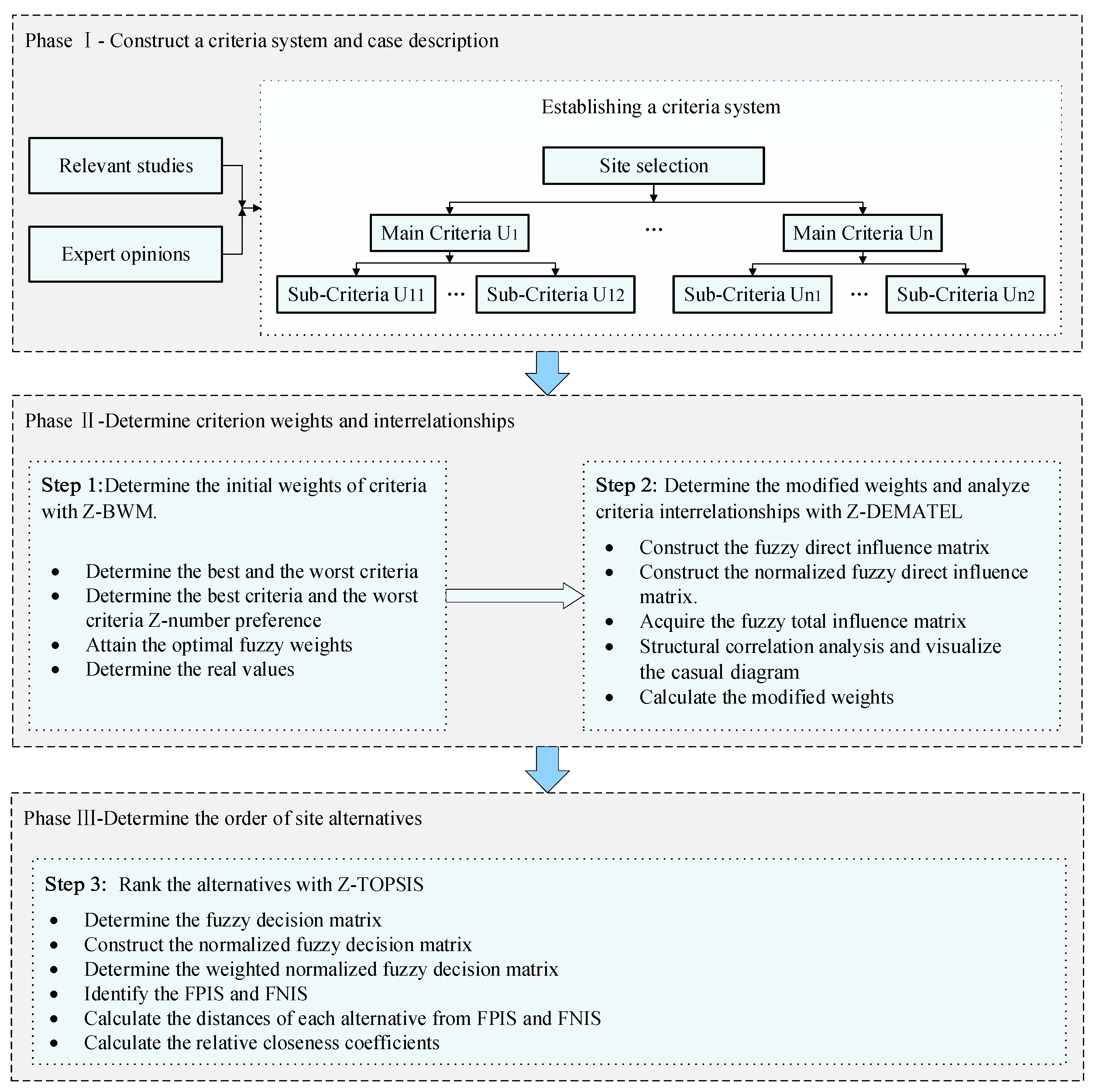
4.1. The Designed Multi-criteria Decision Support Framework

In order to scientifically carry out the location selection project and ensure the creditability of decision-making results, the evaluation framework proposed in this study is divided into three phases: (1) Construct a criteria system and case description; (2) determine criterion weights and interrelationships; (3) determine the order of site alternatives. In phase one, a specific inland NPP indicator framework is established as shown in Section 2.2, which will be the basis for the following phases. In phase two, Z-BWM is applied to obtain the initial weight coefficient of evaluation criteria. Subsequently, it is more important to analyze criteria interrelationships with Z-DEMATEL, and determine the modified weights. In phase three, Z-TOPSIS is used to determine the order of site alternatives. From a methodological point of view, the proposed multi-criteria decision support framework for inland NPP site selection comprises the following steps, as presented in Figure 1.

4.2. The Proposed Methods in the Inland NPP Siting Framework

4.2.1. Phase II: Determine Criterion Weights and Interrelationships

Step 1. Determine the initial weights of criteria with Z-BWM.

BWM is a criterion weights determination method [19]. In the traditional BWM, the evaluation information is usually expressed by using crisp or fuzzy numbers. In view of the subjectivity and fuzziness of group decision-making, BWM is integrated with Z-numbers in this step, and Z-BWM includes the following implementation steps.

Step 1.1. Determine the best and worst criteria.

The best (most important) and the worst (least significant) criteria are determined by decision-makers from their own perspectives.

Step 1.2. Determine the best criteria and the worst criteria Z-number preference.

Linguistic variable is considered as one of the most effective means for dealing with complex or ill-defined situations [44,45]. In this step, decision-makers should rate their preferences using linguistic variables represented by Z-numbers, as shown in

Table 2. The membership function of linguistic terms.

Constraint		Reliability
Linguistic Terms	Fuzzy Numbers	Linguistic Terms	Fuzzy Numbers
Equally Important (EI)	(1,1,1)	Strongly Unlikely (SU)	(0,0,0.3)
Weakly Important (WI)	(2/3,1,3/2)	Unlikely (U)	(0.1,0.3,0.5)
Generally Important (GI)	(3/2,2,5/2)	Neutral (N)	(0.3,0.5,0.7)
Very Important (VI)	(5/2,3,7/2)	Likely (L)	(0.5,0.7,0.9)
Absolutely Important (AI)	(7/2,4,9/2)	Strongly Likely (SL)	(0.7,1.0,1.0)

. By adopting Equations (2)–(4), Z-number linguistic preferences will be transformed into the regular fuzzy ratings except when criterion i and criterion j are equally important. Then, the fuzzy best-to-others (BO) comparison vector ${\tilde{A}}_B=({\tilde{a}}_{B1},{\tilde{a}}_{B2},\cdots ,{\tilde{a}}_{Bj},\dots ,{\tilde{a}}_{Bn})$ and the fuzzy others-to-worst (OW) comparison vector ${\tilde{A}}_W=({\tilde{a}}_{1W},{\tilde{a}}_{2W},\cdots ,{\tilde{a}}_{jW},\dots ,{\tilde{a}}_{nW})$ are obtained. Example of Z-number linguistic variables are:

Assume a Z-number linguistic term “Absolutely Important (AI)” with a reliability “Likely (L).” This is depicted as follows.

$$Z=(\tilde{A},\tilde{B})=(\mathrm{AI},\mathrm{L})=[(7/2,4,9/2),(0.5,0.7,0.9].$$

First, the component $\tilde{B}$ is translated into a crisp number by adopting Equation (2).

$$\alpha =\frac{{\displaystyle \int x{\mu }_{\tilde{B}}(x)dx}}{{\displaystyle \int {\mu }_{\tilde{B}}(x)dx}}=0.7.$$

According to Equations (3) and (4), the weight of reliability is added to the first component $\tilde{A}$. Then, the weighted Z-number ${\tilde{Z}}^{\alpha }$ is converted into a regular fuzzy number.

$${\tilde{Z}}^{\prime }=(\sqrt{0.7}\times 7/2,\sqrt{0.7}\times 4,\sqrt{0.7}\times 9/2)=(2.94,3.36,3.78).$$

Step 1.3. Attain the optimal fuzzy weights.

Based on the principle of minimizing the maximum deviation, the following mathematical programming form is established to calculate the optimal fuzzy weights ${\tilde{W}}^{\ast }=({\tilde{w}}_1^{\ast },\cdots ,{\tilde{w}}_n^{\ast })$.

$$\begin{array}{l}\min {\max }_j\left\{\left|\frac{{\tilde{w}}_B}{{\tilde{w}}_j}-{\tilde{a}}_{Bj}\right|,\left|\frac{{\tilde{w}}_j}{{\tilde{w}}_W}-{\tilde{a}}_{jW}\right|\right\}\\ s.t.\\ {\displaystyle \sum _j{\tilde{w}}_j}=1,\\ m_j^w\le n_j^w\le q_j^w,\\ m_j^w\ge 0,\mathrm{for}\mathrm{all}j,\end{array}$$

(5)

where ${\tilde{W}}_B=(m_B^w,n_B^w,q_B^w)$, ${\tilde{W}}_j=(m_j^w,n_j^w,q_j^w)$, ${\tilde{W}}_W=(m_W^w,n_W^w,q_W^w)$, ${\tilde{a}}_{Bj}=(m_{Bj},n_{Bj},q_{Bj})$ and ${\tilde{a}}_{jW}=(m_{jW},n_{jW},q_{jW})$.

Equation (5) can be transformed into:

$$\begin{array}{l}\min {\epsilon }^L\\ s.t.\\ \left|\frac{{\tilde{w}}_B}{{\tilde{w}}_j}-{\tilde{a}}_{Bj}\right|\le {\epsilon }^L,\mathrm{for}\mathrm{all}j,\\ \left|\frac{{\tilde{w}}_j}{{\tilde{w}}_W}-{\tilde{a}}_{jW}\right|\le {\epsilon }^L,\mathrm{for}\mathrm{all}j,\\ {\displaystyle \sum _j{\tilde{w}}_j}=1,\\ m_j^w\le n_j^w\le q_j^w,\\ m_j^w\ge 0,\mathrm{for}\mathrm{all}j,\end{array}$$

(6)

where ${\epsilon }^L=(m^{\epsilon },n^{\epsilon },q^{\epsilon })$.

Assuming the optimal objective function value ${\epsilon }^{L^{\ast }}=(k^{\ast },k^{\ast },k^{\ast }),k^{\ast }<m^{\epsilon }$, Equation (6) can be transformed into [46]:

$$\begin{array}{l}\min {\epsilon }^{L^{\ast }}\\ s.t.\\ \left|\frac{(m_B^w,n_B^w,q_B^w)}{(m_j^w,n_j^w,q_j^w)}-(m_{Bj,}{n}_{Bj,}{q}_{Bj,})\right|\le (k^{\ast },k^{\ast },k^{\ast }),\\ \left|\frac{(m_j^w,n_j^w,q_j^w)}{(m_W^w,n_W^w,q_W^w)}-(m_{Bj,}{n}_{Bj,}{q}_{Bj,})\right|\le (k^{\ast },k^{\ast },k^{\ast }),\\ {\displaystyle \sum _j{\tilde{w}}_j}=1,\\ m_j^w\le n_j^w\le q_j^w,\\ m_j^w\ge 0,\mathrm{for}\mathrm{all}j.\end{array}$$

(7)

By solving this nonlinear programming model, we can determine the optimal fuzzy weights $({\tilde{w}}_1^{\ast },{\tilde{w}}_2^{\ast },\cdots ,{\tilde{w}}_n^{\ast })$ of evaluation criteria. ${\epsilon }^{L^{\ast }}$ is the consistency index, and its values being closer to zero indicates a higher consistency in the results of pairwise comparisons. The maximum values of ${\epsilon }^{L^{\ast }}$ (consistency index) for different linguistic variables of $a_{BW}$ can be retrieved from

Table 3. Values of the consistency index (CI) for Z-BWM [47].

Linguistic variable	(EI, SU)	(EI, U)	(EI, N)	(EI, L)	(EI, SL)
CI	3	3	3	3	3
Linguistic variable	(WI, SU)	(WI, U)	(WI, N)	(WI, L)	(WI, SL)
CI	2.07	2.7	3.11	3.42	3.68
Linguistic variable	(GI, SU)	(GI, U)	(GI, N)	(GI, L)	(GI, SL)
CI	2.64	3.6	4.22	4.71	5.11
Linguistic variable	(VI, SU)	(VI, U)	(VI, N)	(VI, L)	(VI, SL)
CI	3.17	4.44	5.27	5.92	6.45
Linguistic variable	(AI, SU)	(AI, U)	(AI, N)	(AI, L)	(AI, SL)
CI	3.68	5.24	6.27	7.07	7.74

.

Based on Table 3, the consistency ratio (CR) is obtained as below:

$$\mathrm{CR}=\frac{{\epsilon }^{L^{\ast }}}{\mathrm{CI}}.$$

(8)

Step 1.4. Determine the real values.

Based on the optimal fuzzy weights, the real values $R({\tilde{a}}_i)$ is calculated as below:

$$R({\tilde{a}}_i)=\frac{m_i+4n_i+q_i}{6}.$$

(9)

Step 2. Determine the modified weights and analyze criteria interrelationships with Z-DEMATEL.

DEMATEL is widely applied to visualize the causal relationships of evaluation criteria. Our proposed Z-DEMATEL method is an innovation of the traditional DEMATEL, where the characteristics of both Z-numbers and DEMATEL are remained. The reliability information can be obtained from Table 1, and the criteria comparison linguistic terms are presented in

Table 4. Linguistic variables for criteria comparison.

Linguistic Terms	Fuzzy Numbers
No Influence (NO)	(0,0,0)
Very Low Influence (VL)	(0,0,0.25)
Low Influence (L)	(0,0.25,0.5)
High Influence (H)	(0.25,0.5,0.75)
Very High Influence (VH)	(0.5,0.75,1.0)

[48]. The procedures of Z-DEMATEL are summarized in five steps.

Step 2.1. Construct the fuzzy direct influence matrix.

The fuzzy direct influence matrix ${\tilde{X}}^t$ of all decision-makers are determined using Equations (2)–(4). Supposing a decision group with H persons, the average of experts’ evaluation is extracted by adopting Equation (10).

$${\tilde{X}}^t=\left[\begin{array}{cccc}0& {\tilde{x}}_{12}^t& \cdots & {\tilde{x}}_{1n}^t\\ {\tilde{x}}_{21}^t& 0& \cdots & {\tilde{x}}_{2n}^t\\ ⋮& ⋮& \ddots & ⋮\\ {\tilde{x}}_{n1}^t& {\tilde{x}}_{n2}^t& \cdots & 0\end{array}\right],$$

$$Z={[z_{ij}]}_{n\times n}=\frac{1}{H}{\displaystyle \sum _{k=1}^H{[{\tilde{x}}_{ij}^t]}_{n\times n}}.$$

(10)

Step 2.2. Construct the normalized fuzzy direct influence matrix.

$$D=\frac{Z}{u}=\left(\frac{l_{ij}}{u},\frac{r_{ij}}{u},\frac{u_{ij}}{u}\right)=(l_{ij}^{\prime },r_{ij}^{\prime },u_{ij}^{\prime }),$$

(11)

$$u={\max }_{1\le i\le n}{\displaystyle \sum _{j=1}^n{u}_{ij}}.$$

Step 2.3. Acquire the fuzzy total influence matrix $T$.

$$T=D_l\times {(I-D)}^{-1}=(l_{ij}^t,r_{ij}^t,u_{ij}^t),$$

(12)

where $[l_{ij}^t]=D_l\times {(I-D_l)}^{-1},[r_{ij}^t]=D_r\times {(I-D_r)}^{-1},[u_{ij}^t]=D_u\times {(I-D_u)}^{-1}.$

Step 2.4. Structural correlation analysis and visualize the casual diagram.

Using Equation (13), the sum of rows and columns is expressed as vector $R$ and vector $C$, respectively. After that, the fuzzy ordered pairs $(R+C,R-C)$ are obtained, and the expected values of $E(R+C)$ and $E(R-C)$ are calculated using Equation (9).

$$\begin{array}{l}T={[t_{ij}]}_{n\times n},i,j=1,2,\cdots ,n,\\ R={\left({\displaystyle \sum _{j=1}^n{t}_{ij}}\right)}_{n\times 1},\\ C={\left({\displaystyle \sum _{i=1}^n{t}_{ij}}\right)}_{1\times n}.\end{array}$$

(13)

The initial weights $W_j^{\ast }$ from Step 1.4 are combined with the expected values $E(W)=E(R+C,R-C)$. Then, the new expected values $E(W{)}^{\prime }=E({R_i}^{\prime }+{C_i}^{\prime },{R_i}^{\prime }-{C_i}^{\prime })$ are determined using Equation (14).

$$E(W{)}^{\prime }=W_j^{\ast }\times E(W).$$

(14)

After that, the casual diagrams are constructed with the horizontal axis “prominence” $({R_i}^{\prime }+{C_i}^{\prime })$ and the vertical axis “relation” $({R_i}^{\prime }-{C_i}^{\prime })$. The “prominence” and “relation” indicate the self-importance and net effect of criterion i in the system, respectively. If $({R_i}^{\prime }-{C_i}^{\prime })$ is positive, the factors are causal; otherwise, the factors belong to the effect group.

Step 2.5. Calculate the modified weights $\widehat{W}$.

$$W_{i0}={[{({R_i}^{\prime }+{C_i}^{\prime })}^2+{({R_i}^{\prime }-{C_i}^{\prime })}^2]}^{1/2},$$

(15)

$$\widehat{W}=\frac{W_{i0}}{{\displaystyle \sum _{i=1}^n{W}_{i0}}}.$$

(16)

4.2.2. Phase III: Determine the Order of Site Alternatives

Step 3. Rank the alternatives with Z-TOPSIS.

The traditional TOPSIS was proposed to determine the optimal solution among limited schemes in system engineering. In consideration of the fuzziness of human’s opinion, Chen and Hwang [49] integrated the fuzzy set theory with TOPSIS. As an extension of the classic TOPSIS, fuzzy TOPSIS has been applied in the fields of water resources evaluation, performance evaluation, and solar site selection [50]. In this work, fuzzy TOPSIS is further extended to Z-numbers, and Z-TOPSIS should be carried out as below.

Step 3.1. Determine the fuzzy decision matrix.

In this step, the reliability information obtained from Table 1, and the linguistic terms for alternative ratings are shown in

Table 5. Linguistic variables for alternative ratings.

Linguistic Terms	Fuzzy Numbers
Very Poor (VP)	(1,1,3)
Poor (P)	(1,3,5)
Fairly (F)	(3,5,7)
Good (G)	(5,7,9)
Very Good (VG)	(7,9,9)

. The fuzzy decision matrix $Y_{ij}$ could be constructed by using the arithmetic conversion rules given in Equations (2)–(4).

$$\begin{array}{l}{Y}_{ij}=\left[\begin{array}{cccc}{y}_{11}& y_{12}& \cdots & y_{1n}\\ y_{21}& y_{22}& \cdots & y_{2n}\\ ⋮& ⋮& \ddots & ⋮\\ y_{m1}& y_{m2}& \cdots & y_{mn}\end{array}\right],\\ {\tilde{y}}_{ij}=\frac{1}{H}[{\tilde{y}}_{ij}^1+{\tilde{y}}_{ij}^2+\cdots +{\tilde{y}}_{ij}^H],\end{array}$$

(17)

where ${\tilde{y}}_{ij}^H$ is the rating given by the $H\mathrm{th}$ decision-maker, and $y_{ij}=(a_{ij},b_{ij},c_{ij}).$

Step 3.2. Construct the normalized fuzzy decision matrix.

$$\begin{array}{l}\tilde{R}={[{\tilde{r}}_{ij}]}_{m\times n},\\ {\tilde{r}}_{ij}=\left(\frac{a_{ij}}{c_j^{\ast }},\frac{b_{ij}}{c_j^{\ast }},\frac{c_{ij}}{c_j^{\ast }}\right),j\in B,\\ {\tilde{r}}_{ij}=\left(\frac{a_j^{-}}{c_{ij}},\frac{a_j^{-}}{b_{ij}},\frac{a_j^{-}}{a_{ij}}\right),j\in C,\\ c_j^{\ast }={\max }_i{c}_{ij}\mathrm{if}j\in B,\\ a_j^{\ast }={\min }_i{a}_{ij}\mathrm{if}j\in C.\end{array}$$

(18)

Step 3.3. Determine the weighted normalized fuzzy decision matrix.

$$\begin{array}{l}\tilde{V}={[{\tilde{v}}_{ij}]}_{m\times n},i=1,2,\cdots ,m,\mathrm{and}j=1,2,\cdots ,n,\\ {\tilde{v}}_{ij}={\tilde{r}}_{ij}\times {\widehat{w}}_j.\end{array}$$

(19)

Step 3.4. Identify the fuzzy positive-ideal solution (FPIS) and negative-ideal solution (FNIS).

$$\begin{array}{l}{A}^{\ast }=(\stackrel{~\ast }{v_1},\stackrel{~\ast }{v_2},\cdots ,\stackrel{~\ast }{v_n}),\\ A^{-}=(\stackrel{~-}{v_1},\stackrel{~-}{v_2},\cdots ,\stackrel{~-}{v_n}),\end{array}$$

(20)

where $\stackrel{~\ast }{v_j}=(1,1,1)$ and $\stackrel{~-}{v_j}=(0,0,0)$ for $j=1,2,\cdots ,n.$

Step 3.5. Calculate the distances of each alternative from FPIS $A^{\ast }$ and FNIS $A^{-}$.

$$\begin{array}{l}{d}_i^{\ast }={\displaystyle \sum _{j=1}^{n}d({\tilde{v}}_{ij},\stackrel{~\ast }{v_j})},i=1,2,\cdots ,m,\mathrm{and}j=1,2,\cdots n,\\ d_i^{-}={\displaystyle \sum _{j=1}^{n}d({\tilde{v}}_{ij},\stackrel{~-}{v_j})},i=1,2,\cdots ,m,\mathrm{and}j=1,2,\cdots n,\end{array}$$

(21)

where the distance between $\tilde{Y}=(f_1,f_2,f_3)$ and $\tilde{Z}=(z_1,z_2,z_3)$ can be calculated as:

$$d(\tilde{F},\tilde{Z})=\sqrt{\frac{1}{3}[{(f_1-z_1)}^2+{(f_2-z_2)}^2+{(f_3-z_3)}^2]}.$$

Step 3.6. Calculate the relative closeness coefficients.

$$C{C}_i=\frac{d_i^{-}}{d_i^{\ast }+d_i^{-}},i=1,2,\cdots ,m,\mathrm{and}C{C}_i\in (0,1).$$

(22)

5. Case Study and Result

As shown in Figure 2 (right-hand side), Hunan is one of provinces in central China, with its location around 28.19° N and 112.98° E. It covers an area of 211,800 square kilometers and has a population of more than 6.7372 million people. The demand of energy is going up with the increase of population and economy in this province. Most of Hunan’s electricity is generated from fossil fuels, predominantly from coal—which accounted for 55.3% in 2019 The next is hydropower, accounting for 31.1%. Only 13.6% of the total installed generating capacity comes from new energy resources like the sun or wind. In recent years, the electricity consumption per capita in this area is only about 62.4% of the national level. Considering the current electricity shortage in Hunan province, there could be a strategy to develop nuclear power for the future of regional energy industry. In addition, Hunan province has one unique advantage in NPP construction. It locates outside of fault lines, where four first-order stream (Xiang, Zi, Yuan, and Li) in the territory has abundant cooling water resources. The rapid progress of China’s nuclear power also makes a solid technical basis for the development of Hunan’s nuclear power industry. According to China’s inland nuclear power development plan, the distribution of the selected locations is shown in Figure 2 (left-hand side). In this work, we use S₁, S₂, S₃, S₄, S₅, and S₆ to represent Jiulongshan, Taoyuan, Huarong, Xiangyin, Taojiang, and Sanzhang, respectively.

5.1. Phase I: Construct A Criteria System and Case Description

Determination of the siting criteria for inland NPPs is the primary step in the proposed decision framework. Evaluation criteria includes three main dimensions and 16 sub-criteria (Table 1). Four professionals being engaged in nuclear-energy, electricity, geography, and economics are invited to form a decision panel. The average working life of every expert is more than 10 years and they all have rich experiences in the nuclear power industry. In addition, since every expert has distinguishing characteristics and roles in the decision process, the same importance weight is assigned to them. The interrelationships and weights of evaluation criteria can be determined on the basis of expert opinions.

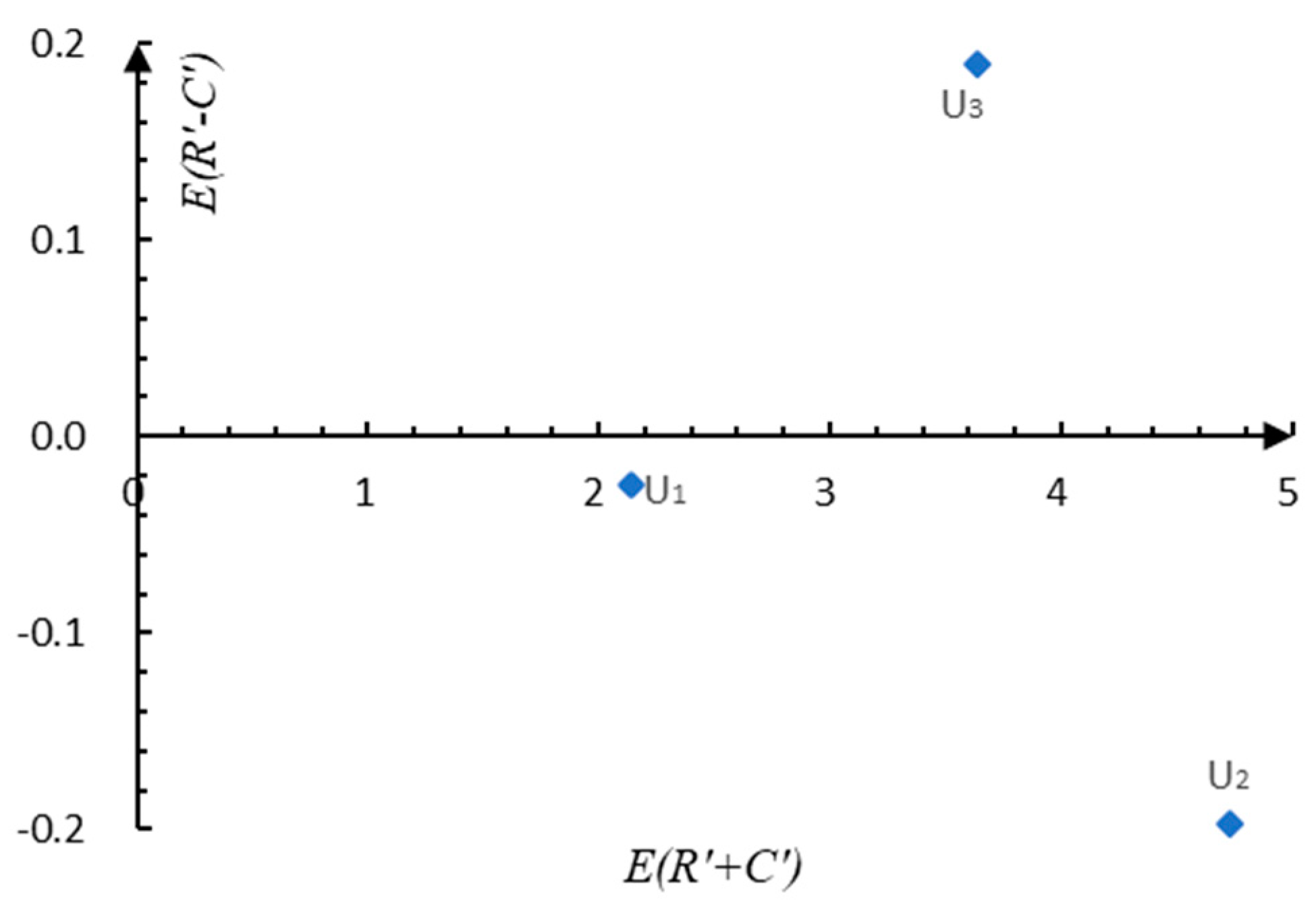
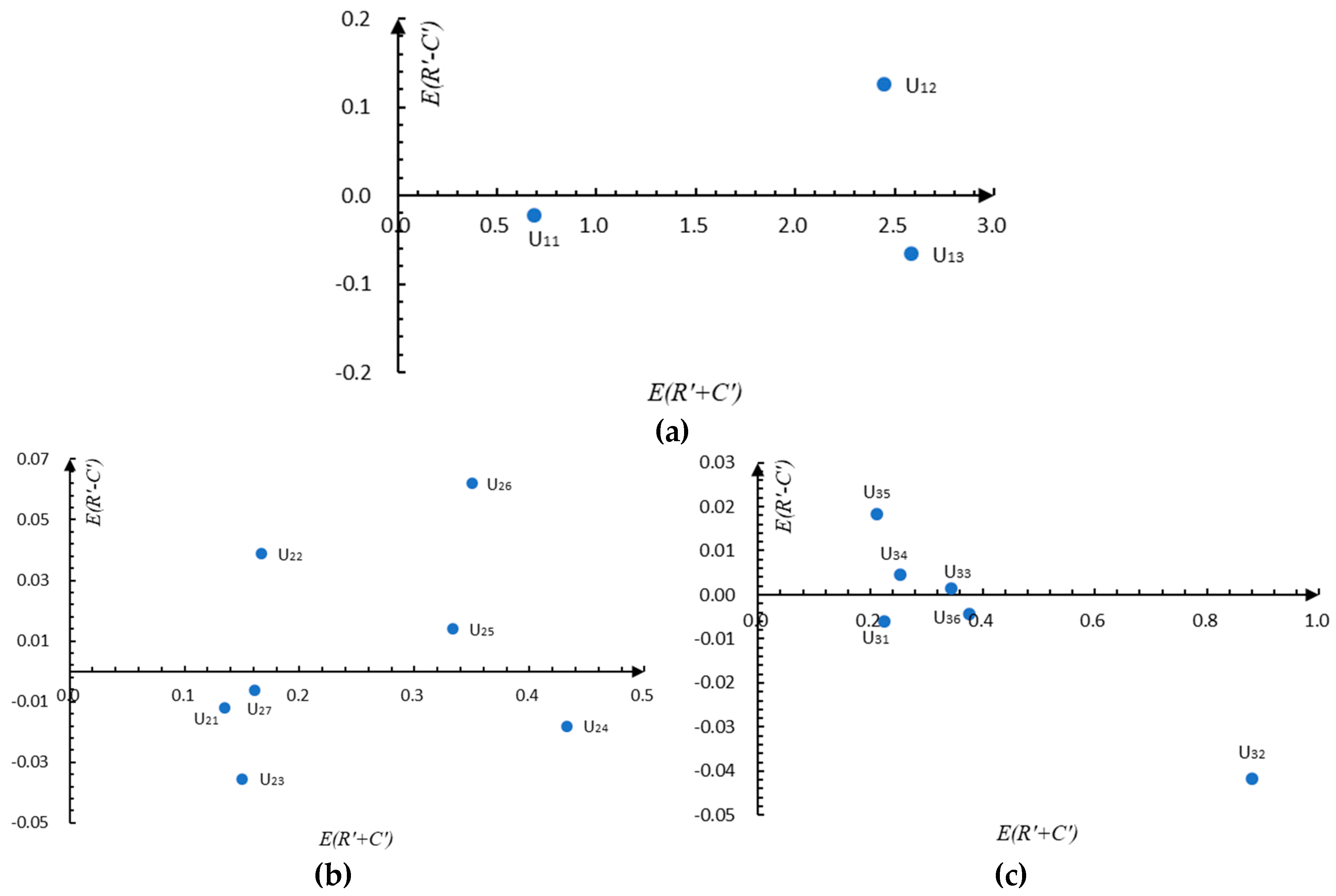
5.2. Phase II: Determine Criterion Weights and Interrelationships

Step 1. Determine the initial weights of criteria with Z-BWM.

Step 1.1. Determine the best and worst criteria.

On the basis of judgment from decision panel, the best criteria and worst criteria are presented in

Table 6. The best and worst criteria of the main criteria.

	DM1	DM2	DM3	DM4
Best criteria	U2	U2	U3	U1
Worst criteria	U1	U1	U1	U3

and

Table 7. The best and worst criteria of sub-criteria.

		DM1	DM2	DM3	DM4
U1	Best criteria	U12	U13	U13	U12
	Worst criteria	U11	U11	U11	U11
U2	Best criteria	U25	U26	U25	U24
	Worst criteria	U23	U22	U22	U21
U3	Best criteria	U32	U32	U32	U32
	Worst criteria	U35	U31	U34	U31

.

Step 1.2. Determine the best criteria and the worst criteria Z-number preference.

The BO (${\tilde{A}}_B$) and the OW (${\tilde{A}}_W$) vectors of the main criteria are shown as

Table 8. The linguistic preference comparison vectors.

	Best-to-Others Vectors			Others-to-Worst Vectors
	U1	U2	U3	U1	U2	U3
DM1	(AI, L)	(EI, SL)	(GI, L)	(EI, SL)	(AI, L)	(VI, L)
DM2	(AI, L)	(EI, L)	(VI, U)	(EI, L)	(AI, L)	(VI, N)
DM3	(VI, SL)	(WI, L)	(EI, SL)	(EI, SL)	(VI, L)	(VI, SL)
DM4	(EI, L)	(WI, N)	(GI, L)	(GI, L)	(GI, U)	(EI, L)

. According to Equations (2)–(4), the fuzzy best-to-others and the others-to-worst vectors of the main criteria are presented in

Table 9. The fuzzy preference comparison vectors.

	Best-to-Others Vectors
	U1	U2	U3
DM1	(2.94,3.36,3.78)	(1,1,1)	(1.26,1.68,2.10)
DM2	(2.94,3.36,3.78)	(1,1,1)	(1.37,1.64,1.92)
DM3	(2.38,2.85,3.33)	(0.56,0.84,1.26)	(1,1,1)
DM4	(1,1,1)	(0.47,0.71,0.82)	(1.26,1.68,2.10)
	Others-to-Worst Vectors
	U1	U2	U3
DM1	(1,1,1)	(2.94,3.36,3.78)	(2.10,2.52,2.94)
DM2	(1,1,1)	(2.94,3.36,3.78)	(1.78,2.13,2.49)
DM3	(1,1,1)	(2.10,2.52,2.94)	(2.38,2.85,3.33)
DM4	(1.26,1.68,2.10)	(0.82,1.10,1.37)	(1,1,1)

.

Steps 1.3 and 1.4. Attain the optimal fuzzy weights and determine the real values.

On the basis of Equations (5)–(7), the following models 1–4 are constructed to calculate the optimal fuzzy weights of main criteria, and presented in

Table 10. The optimal fuzzy weights.

	U1	U2	U3	${\mathit{k}}^{\ast }$
DM1	(0.138,0.147,0.147)	(0.458,0.520,0.546)	(0.283,0.345,0.382)	(0.174,0.174,0.174)
DM2	(0.141,0.157,0.158)	(0.467,0.532,0.532)	(0.277,0.330,0.348)	(0.028,0.028,0.028)
DM3	(0.156,0.157,0.157)	(0.347,0.422,0.484)	(0.349,0.423,0.494)	(0.162,0.162,0.162)
DM4	(0.302,0.368,0.409)	(0.361,0.361,0.385)	(0.229,0.269,0.319)	(0.313,0.313,0.313)

$$\begin{array}{l}\mathrm{Model}1\min k^{1\ast }\\ s.t.\{\begin{array}{l}-k^{1\ast }\ast q_1\le m_2-2.94\ast q_1\le k^{1\ast }\ast q_1\\ -k^{1\ast }\ast n_1\le n_2-3.36\ast n_1\le k^{1\ast }\ast n_1\\ -k^{1\ast }\ast m_1\le q_2-3.78\ast m_1\le k^{1\ast }\ast m_1\\ -k^{1\ast }\ast q_3\le m_2-1.26\ast q_3\le k^{1\ast }\ast q_3\\ -k^{1\ast }\ast n_3\le n_2-1.68\ast n_3\le k^{1\ast }\ast n_3\\ -k^{1\ast }\ast m_3\le q_2-2.1\ast m_3\le k^{1\ast }\ast m_3\\ -k^{1\ast }\ast q_1\le m_3-2.1\ast q_1\le k^{1\ast }\ast q_1\\ -k^{1\ast }\ast n_1\le n_3-2.52\ast n_1\le k^{1\ast }\ast n_1\\ -k^{1\ast }\ast m_1\le q_3-2.94\ast m_1\le k^{1\ast }\ast m_1\\ 1/6\ast (m_1+m_2+m_3)+4/6\ast (n_1+n_2+n_3)\\ +1/6\ast (q_1+q_2+q_3)\\ m_j\le n_j\le q_j,\forall j=1,2,3\\ m_j>0,\forall j=1,2,3\\ k^{1\ast }\ge 0\end{array},\end{array}$$

$$\begin{array}{l}\mathrm{Model}2\min k^{2\ast }\\ s.t.\{\begin{array}{l}-k^{2\ast }\ast q_1\le m_2-2.94\ast q_1\le k^{2\ast }\ast q_1\\ -k^{2\ast }\ast n_1\le n_2-3.36\ast n_1\le k^{2\ast }\ast n_1\\ -k^{2\ast }\ast m_1\le q_2-3.78\ast m_1\le k^{2\ast }\ast m_1\\ -k^{2\ast }\ast q_3\le m_2-1.37\ast q_3\le k^{2\ast }\ast q_3\\ -k^{2\ast }\ast n_3\le n_2-1.64\ast n_3\le k^{2\ast }\ast n_3\\ -k^{2\ast }\ast m_3\le q_2-1.92\ast m_3\le k^{2\ast }\ast m_3\\ -k^{2\ast }\ast q_1\le m_3-1.78\ast q_1\le k^{2\ast }\ast q_1\\ -k^{2\ast }\ast n_1\le n_3-2.13\ast n_1\le k^{2\ast }\ast n_1\\ -k^{2\ast }\ast m_1\le q_3-2.49\ast m_1\le k^{2\ast }\ast m_1\\ 1/6\ast (m_1+m_2+m_3)+4/6\ast (n_1+n_2+n_3)\\ +1/6\ast (q_1+q_2+q_3)\\ m_j\le n_j\le q_j,\forall j=1,2,3\\ m_j>0,\forall j=1,2,3\\ k^{2\ast }\ge 0\end{array},\end{array}$$

$$\begin{array}{l}\mathrm{Model}3\min k^{3\ast }\\ s.t.\{\begin{array}{l}-k^{3\ast }\ast q_1\le m_3-2.38\ast q_1\le k^{3\ast }\ast q_1\\ -k^{3\ast }\ast n_1\le n_3-2.85\ast n_1\le k^{3\ast }\ast n_1\\ -k^{3\ast }\ast m_1\le q_3-3.33\ast m_1\le k^{3\ast }\ast m_1\\ -k^{3\ast }\ast q_2\le m_3-0.56\ast q_2\le k^{3\ast }\ast q_2\\ -k^{3\ast }\ast n_2\le n_3-0.84\ast n_2\le k^{3\ast }\ast n_2\\ -k^{3\ast }\ast m_2\le q_3-1.26\ast m_2\le k^{3\ast }\ast m_2\\ -k^{3\ast }\ast q_1\le m_2-2.1\ast q_1\le k^{3\ast }\ast q_1\\ -k^{3\ast }\ast n_1\le n_2-2.52\ast n_1\le k^{3\ast }\ast n_1\\ -k^{3\ast }\ast m_1\le q_2-2.94\ast m_1\le k^{3\ast }\ast m_1\\ 1/6\ast (m_1+m_2+m_3)+4/6\ast (n_1+n_2+n_3)\\ +1/6\ast (q_1+q_2+q_3)\\ m_j\le n_j\le q_j,\forall j=1,2,3\\ m_j>0,\forall j=1,2,3\\ k^{3\ast }\ge 0\end{array},\end{array}$$

$$\begin{array}{l}\mathrm{Model}4\min k^{4\ast }\\ s.t.\{\begin{array}{l}-k^{4\ast }\ast q_2\le m_1-0.47\ast q_2\le k^{4\ast }\ast q_2\\ -k^{4\ast }\ast n_2\le n_1-0.71\ast n_2\le k^{4\ast }\ast n_2\\ -k^{4\ast }\ast m_2\le q_1-0.82\ast m_2\le k^{4\ast }\ast m_2\\ -k^{4\ast }\ast q_3\le m_1-1.26\ast q_3\le k^{4\ast }\ast q_3\\ -k^{4\ast }\ast n_3\le n_1-1.68\ast n_3\le k^{4\ast }\ast n_3\\ -k^{4\ast }\ast m_3\le q_1-2.1\ast m_3\le k^{4\ast }\ast m_3\\ -k^{4\ast }\ast q_3\le m_2-0.82\ast q_3\le k^{4\ast }\ast q_3\\ -k^{4\ast }\ast n_3\le n_2-1.1\ast n_3\le k^{4\ast }\ast n_3\\ -k^{4\ast }\ast m_3\le q_2-1.37\ast m_3\le k^{4\ast }\ast m_3\\ 1/6\ast (m_1+m_2+m_3)+4/6\ast (n_1+n_2+n_3)\\ +1/6\ast (q_1+q_2+q_3)\\ m_j\le n_j\le q_j,\forall j=1,2,3\\ m_j>0,\forall j=1,2,3\\ k^{4\ast }\ge 0\end{array}.\end{array}$$

Based on Equation (8) and Table 3, the consistency ratios are 0.174/7.07 = 0.025, 0.028/7.07 = 0.004, 0.162/6.45 = 0.025, and 0.313/4.71 = 0.066, and all of them are less than 0.1. According to Equation (9), the crisp weights of the main criteria evaluated by four experts are (0.145,0.514,0.341), (0.155,0.521,0.324), (0.157,0.420,0.423), and (0.364,0.365,0.271). Since the same weight is assigned to every expert, the final optimal weights are calculated as follows.

$$w_1^{\ast }=(w_1^{1\ast }+w_1^{2\ast }+w_1^{3\ast }+w_1^{4\ast })/4=(0.145+0.155+0.157+0.364)/4=0.205,$$

$$w_2^{\ast }=(w_2^{1\ast }+w_2^{2\ast }+w_2^{3\ast }+w_2^{4\ast })/4=(0.514+0.521+0.42+0.365)/4=0.455,$$

$$w_3^{\ast }=(w_3^{1\ast }+w_3^{2\ast }+w_3^{3\ast }+w_3^{4\ast })/4=(0.341+0.324+0.423+0.271)/4=0.34.$$

The optimal weights of all sub-criteria are calculated in a similar way as described above. After that, we can determine the final weights of all sub-criteria, and multiply the real value of the main criteria by the optimal weights of sub-criteria. Finally, the global weights of sub-criteria are obtained, as shown in

Table 11. The global weights of sub-criteria.

Main Criteria	Sub-criteria	Final Weights	Global Weights
U1	U11	0.144	0.030
	U12	0.413	0.084
	U13	0.443	0.091
U2	U21	0.078	0.035
	U22	0.091	0.042
	U23	0.074	0.034
	U24	0.203	0.092
	U25	0.220	0.100
	U26	0.218	0.099
	U27	0.117	0.053
U3	U31	0.113	0.038
	U32	0.309	0.105
	U33	0.153	0.052
	U34	0.116	0.039
	U35	0.114	0.039
	U36	0.196	0.067

.

Step 2. Determine the modified weights and analyze criteria interrelationships with Z-DEMATEL.

Step 2.1. Construct the fuzzy direct influence matrix.

The decision-makers use Z-number linguistic variables to make pairwise comparisons and analyze the degree of interrelationship among the main criteria. The Z-number linguistic variables direct influence matrix is shown in

Table 12. The Z-number linguistic variables direct influence matrix.

	DM1			DM2
	U1	U2	U3	U1	U2	U3
U1	(NO, SU)	(H, L)	(L, SL)	(NO, SU)	(H, L)	(L, L)
U2	(L, L)	(NO, SU)	(H, L)	(VL, L)	(NO, SU)	(H, N)
U3	(VH, N)	(L, SL)	(NO, SU)	(H, SL)	(H, L)	(NO, SU)
	DM3			DM4
	U1	U2	U3	U1	U2	U3
U1	(NO, SU)	(L, L)	(H, N)	(NO, SU)	(L, N)	(L, L)
U2	(VH, U)	(NO, SU)	(H, N)	(H, N)	(NO, SU)	(VL, L)
U3	(L, N)	(L, L)	(NO, SU)	(L, SL)	(H, N)	(NO, SU)

. After that, the fuzzy direct influence matrix is obtained (

Table 13. The fuzzy direct influence matrix.

	U1	U2	U3
U1	(0,0,0)	(0.11,0.31,0.51)	(0.05,0.25,0.46)
U2	(0.11,0.24,0.43)	(0,0,0)	(0.14,0.28,0.48)
U3	(0.15,0.36,0.56)	(0.10,0.31,0.51)	(0,0,0)

).

Step 2.2. Construct the normalized fuzzy direct influence matrix.

In this step, the values in Table 13 are transformed into the normalized fuzzy direct influence matrix using Equation (11), as presented in

Table 14. The normalized fuzzy direct influence matrix.

	U1	U2	U3
U1	(0,0,0)	(0.108,0.304,0.500)	(0.049,0.245,0.451)
U2	(0.108,0.235,0.422)	(0,0,0)	(0.137,0.275,0.471)
U3	(0.147,0.353,0.549)	(0.098,0.304,0.500)	(0,0,0)

.

Step 2.3. Acquire the fuzzy total influence matrix.

According to Equation (12), the fuzzy total influence matrix is determined, as presented in

Table 15. The fuzzy total influence matrix.

	U1	U2	U3
U1	(0.022,0.288,8.386)	(0.117,0.532,8.908)	(0.066,0.462,8.428)
U2	(0.133,0.467,8.356)	(0.029,0.284,8.237)	(0.147,0.467,8.119)
U3	(0.163,0.597,9.331)	(0.118,0.578,9.509)	(0.024,0.305,8.686)

.

Steps 2.4 and 2.5. Structural correlation analysis and visualize the casual diagram.

On the basis of Table 15, the sum of rows ($R$) and columns ($C$) are calculated for structural correlation analysis. The expected values of $E(R+C)$ and $E(R-C)$ are determined by Equation (9), and then the new expected values $E(R^{\prime }+C^{\prime })$ and $E(R^{\prime }-C^{\prime })$ are obtained by Equation (14), as shown in

Table 16. The new expected values.

	$\mathit{R}$	$\mathit{C}$	$\mathit{E}(\mathit{R}+\mathit{C})$	$\mathit{E}(\mathit{R}-\mathit{C})$	$\mathit{E}({\mathit{R}}^{\prime }+{\mathit{C}}^{\prime })$	$\mathit{E}({\mathit{R}}^{\prime }-{\mathit{C}}^{\prime })$
U1	(0.205,1.282,25.722)	(0.318,1.352,26.073)	10.476	−0.124	2.148	−0.025
U2	(0.309,1.218,24.712)	(0.264,1.394,26.654)	10.398	−0.434	4.731	−0.197
U3	(0.305,1.480,27.526)	(0.237,1.234,25.233)	10.693	0.558	3.636	0.190

. The casual diagram of the main criteria is shown in Figure 3.

Step 2.6. Calculate the modified weights.

The modified weights of the main criteria are determined by using Equations (15) and (16), and we obtain ${\widehat{W}}_1=0.204$, ${\widehat{W}}_2=0.45$, and ${\widehat{W}}_3=0.346$. Given space limitations, this paper omits similar steps, and the modified weights of all evaluation criteria are given in

Table 17. The modified weights of evaluation criteria.

Main Criteria	Sub-criteria	Modified Weights
U1 (0.204)	U11 (0.120)	0.024
	U12 (0.428)	0.087
	U13 (0.452)	0.092
U2 (0.45)	U21 (0.078)	0.035
	U22 (0.098)	0.044
	U23 (0.089)	0.040
	U24 (0.248)	0.112
	U25 (0.191)	0.086
	U26 (0.204)	0.092
	U27 (0.092)	0.042
U3 (0.346)	U31 (0.098)	0.034
	U32 (0.384)	0.133
	U33 (0.150)	0.052
	U34 (0.110)	0.038
	U35 (0.093)	0.032
	U36 (0.164)	0.057

. In addition, the casual diagrams of sub-criteria are depicted in Figure 4.

$$W_{10}={[{2.148}^2+{(-0.025)}^2]}^{1/2}=2.148,$$

$$W_{20}={[{4.731}^2+{(-0.197)}^2]}^{1/2}=4.735,$$

$$W_{30}={[{3.636}^2+{(0.19)}^2]}^{1/2}=3.641,$$

$${\widehat{W}}_1=\frac{W_{10}}{{\displaystyle \sum _{i=1}^3{W}_{i0}}}=0.204,$$

$${\widehat{W}}_2=\frac{W_{20}}{{\displaystyle \sum _{i=1}^3{W}_{i0}}}=0.45,$$

$${\widehat{W}}_3=\frac{W_{30}}{{\displaystyle \sum _{i=1}^3{W}_{i0}}}=0.346.$$

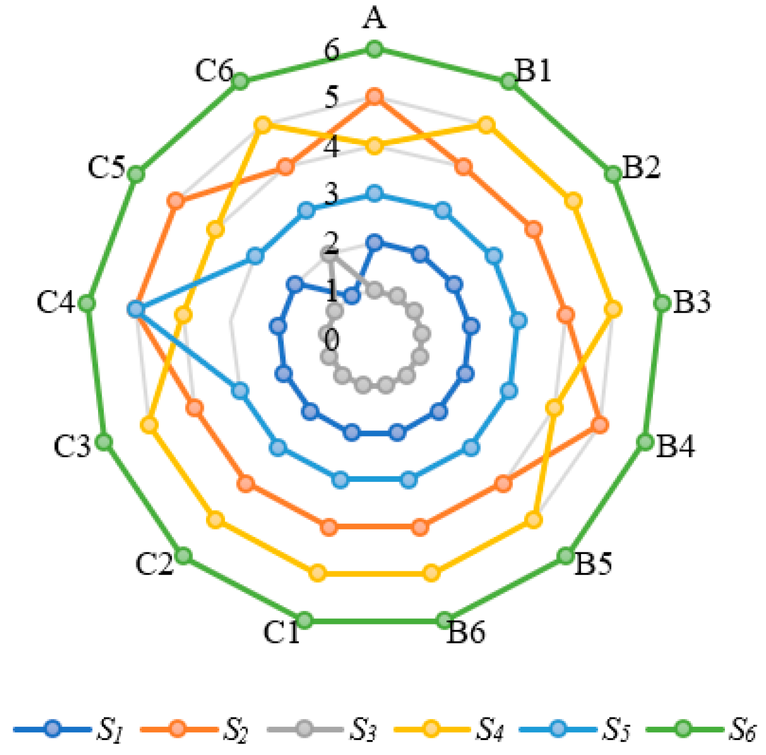
5.3. Phase III: Determine the Order of Site Alternatives

Step 3. Rank the alternatives with Z-TOPSIS.

Steps 3.1–3.3. Obtain the fuzzy decision matrix and determine the weighted normalized fuzzy decision matrix.

The decision panel of this research obtained the fuzzy decision matrix by using the Z-number linguistic variables. After the linguistic variables are converted into triangular fuzzy numbers, the aggregated fuzzy decision matrix is determined by using Equation (17), as shown in

Table A1. The fuzzy decision matrix.

	S1	S2	S3	S4	S5	S6
U11	(2.85,4.51,6.18)	(2.84,4.49,6.15)	(4.32,6.06,7.78)	(4.44,6.22,8.00)	(3.70,5.18,6.65)	(3.85,5.58,7.31)
U12	(3.11,4.71,6.31)	(2.93,4.60,6.28)	(3.07,4.65,6.24)	(2.46,4.18,5.90)	(3.49,5.07,6.66)	(3.37,4.90,6.43)
U13	(3.11,4.71,6.31)	(3.10,4.88,6.67)	(3.67,5.32,6.98)	(2.69,4.29,5.89)	(4.46,6.25,8.04)	(4.18,5.90,7.27)
U21	(3.60,5.21,6.82)	(3.70,5.18,6.65)	(4.65,6.38,7.74)	(3.69,5.35,7.02)	(4.32,6.06,7.78)	(4.04,5.83,7.62)
U22	(3.99,5.78,7.56)	(3.69,5.35,7.02)	(3.43,5.16,6.89)	(3.19,4.79,6.40)	(3.34,4.67,6.00)	(3.70,5.18,6.65)
U23	(2.41,4.02,5.63)	(2.08,3.74,5.41)	(1.95,3.49,5.02)	(0.87,2.18,3.90)	(2.02,3.69,5.35)	(1.70,3.43,5.16)
U24	(0.81,2.00,3.60)	(2.77,4.60,6.45)	(1.26,2.93,4.60)	(2.12,3.54,4.95)	(2.67,4.21,5.76)	(3.18,5.02,6.86)
U25	(0.84,2.50,4.16)	(1.19,2.85,4.51)	(0.84,0.84,2.50)	(0.84,2.09,3.76)	(2.17,3.88,5.60)	(1.31,3.10,4.88)
U26	(3.99,5.78,7.56)	(4.46,6.25,8.04)	(6.25,8.04,8.04)	(4.21,5.76,6.95)	(4.14,5.80,7.45)	(4.14,5.80,7.45)
U27	(3.84,5.37,6.91)	(3.50,4.90,6.30)	(4.74,6.47,7.78)	(3.17,4.62,6.07)	(4.16,5.83,7.49)	(2.82,4.51,6.21)
U31	(0.81,2.00,3.60)	(1.24,3.02,4.79)	(1.19,2.32,3.86)	(2.77,4.60,6.45)	(1.66,3.18,4.70)	(2.50,4.16,5.83)
U32	(0.84,2.51,4.18)	(2.02,3.69,5.35)	(0.80,2.40,4.00)	(2.94,4.65,6.38)	(2.12,3.54,4.95)	(2.77,4.37,5.99)
U33	(0.84,0.84,2.51)	(0.87,2.60,4.32)	(1.16,2.28,3.88)	(0.86,2.11,3.83)	(0.84,2.09,3.76)	(1.45,2.93,4.41)
U34	(4.60,6.45,8.29)	(4.32,6.06,7.78)	(4.93,6.60,7.49)	(3.70,5.18,6.65)	(3.60,5.21,6.82)	(3.53,5.13,6.72)
U35	(2.29,4.13,5.97)	(0.87,2.18,3.90)	(1.51,3.11,4.71)	(0.89,2.67,4.44)	(1.51,3.11,4.71)	(1.73,3.52,5.30)
U36	(4.44,6.05,7.24)	(3.49,5.07,6.66)	(4.35,5.95,7.20)	(2.74,4.37,6.02)	(4.30,6.02,7.74)	(3.37,4.90,6.43)

(see Appendix A). Using the modified weights in Table 17, the fuzzy normalized decision matrix and the weighted normalized fuzzy decision matrix are obtained, as shown in

Table A2. The normalized fuzzy decision matrix.

	S1	S2	S3	S4	S5	S6
U11	(0.357,0.564,0.773)	(0.355,0.562,0.768)	(0.540,0.757,0.973)	(0.555,0.777,1.000)	(0.463,0.647,0.832)	(0.481,0.698,0.913)
U12	(0.467,0.706,0.947)	(0.440,0.691,0.943)	(0.461,0.699,0.937)	(0.370,0.628,0.886)	(0.524,0.762,1.000)	(0.506,0.735,0.965)
U13	(0.387,0.585,0.784)	(0.385,0.607,0.829)	(0.456,0.662,0.868)	(0.335,0.533,0.732)	(0.555,0.777,1.000)	(0.520,0.734,0.904)
U21	(0.463,0.670,0.877)	(0.476,0.665,0.855)	(0.598,0.819,0.995)	(0.474,0.688,0.902)	(0.555,0.778,1.000)	(0.520,0.749,0.979)
U22	(0.527,0.764,1.000)	(0.488,0.708,0.928)	(0.454,0.683,0.911)	(0.421,0.634,0.847)	(0.442,0.618,0.794)	(0.489,0.685,0.880)
U23	(0.154,0.216,0.361)	(0.161,0.232,0.418)	(0.173,0.250,0.446)	(0.223,0.400,1.000)	(0.163,0.236,0.430)	(0.169,0.254,0.511)
U24	(0.225,0.406,1.000)	(0.126,0.176,0.293)	(0.176,0.277,0.644)	(0.164,0.229,0.382)	(0.141,0.192,0.303)	(0.118,0.161,0.255)
U25	(0.202,0.336,1.000)	(0.186,0.294,0.707)	(0.336,1.000,1.000)	(0.223,0.401,1.000)	(0.284,0.403,0.673)	(0.172,0.271,0.640)
U26	(0.496,0.718,0.940)	(0.555,0.777,1.000)	(0.777,1.000,1.000)	(0.524,0.716,0.864)	(0.515,0.721,0.927)	(0.515,0.721,0.927)
U27	(0.494,0.691,0.888)	(0.450,0.629,0.809)	(0.609,0.832,1.000)	(0.407,0.594,0.781)	(0.535,0.749,0.963)	(0.363,0.580,0.799)
U31	(0.225,0.406,1.000)	(0.169,0.268,0.652)	(0.210,0.350,0.679)	(0.126,0.176,0.293)	(0.172,0.255,0.487)	(0.139,0.195,0.324)
U32	(0.191,0.319,0.952)	(0.149,0.217,0.396)	(0.200,0.333,1.000)	(0.125,0.172,0.272)	(0.162,0.226,0.377)	(0.134,0.183,0.289)
U33	(0.335,1.000,1.000)	(0.194,0.324,0.968)	(0.216,0.368,0.727)	(0.219,0.399,0.974)	(0.223,0.401,1.000)	(0.191,0.287,0.580)
U34	(0.555,0.777,1.000)	(0.521,0.730,0.939)	(0.595,0.796,0.903)	(0.446,0.625,0.802)	(0.435,0.629,0.823)	(0.426,0.618,0.811)
U35	(0.146,0.211,0.380)	(0.223,0.400,1.000)	(0.185,0.280,0.577)	(0.196,0.326,0.978)	(0.185,0.280,0.577)	(0.164,0.248,0.503)
U36	(0.574,0.782,0.935)	(0.451,0.655,0.860)	(0.562,0.769,0.930)	(0.354,0.565,0.777)	(0.556,0.778,1.000)	(0.435,0.633,0.831)

and

Table A3. The weighted normalized fuzzy decision matrix.

	S1	S2	S3	S4	S5	S6
U11	(0.009,0.014,0.019)	(0.009,0.013,0.018)	(0.013,0.018,0.023)	(0.013,0.019,0.024)	(0.011,0.016,0.020)	(0.012,0.017,0.022)
U12	(0.041,0.061,0.082)	(0.038,0.060,0.082)	(0.040,0.061,0.082)	(0.032,0.055,0.077)	(0.046,0.066,0.087)	(0.044,0.064,0.084)
U13	(0.036,0.054,0.072)	(0.035,0.056,0.076)	(0.042,0.061,0.080)	(0.031,0.049,0.067)	(0.051,0.072,0.092)	(0.048,0.068,0.083)
U21	(0.016,0.023,0.031)	(0.017,0.023,0.030)	(0.021,0.029,0.035)	(0.017,0.024,0.032)	(0.019,0.027,0.035)	(0.018,0.026,0.034)
U22	(0.023,0.034,0.044)	(0.021,0.031,0.041)	(0.020,0.030,0.040)	(0.019,0.028,0.037)	(0.019,0.027,0.035)	(0.022,0.030,0.039)
U23	(0.006,0.009,0.014)	(0.006,0.009,0.017)	(0.007,0.010,0.018)	(0.009,0.016,0.040)	(0.007,0.009,0.017)	(0.007,0.010,0.020)
U24	(0.025,0.045,0.112)	(0.014,0.020,0.033)	(0.020,0.031,0.072)	(0.018,0.026,0.043)	(0.016,0.022,0.034)	(0.013,0.018,0.029)
U25	(0.017,0.029,0.086)	(0.016,0.025,0.061)	(0.029,0.086,0.086)	(0.019,0.035,0.086)	(0.024,0.035,0.058)	(0.015,0.023,0.055)
U26	(0.046,0.066,0.087)	(0.051,0.072,0.092)	(0.072,0.092,0.092)	(0.048,0.066,0.079)	(0.047,0.066,0.085)	(0.047,0.066,0.085)
U27	(0.020,0.028,0.036)	(0.018,0.026,0.033)	(0.025,0.034,0.041)	(0.017,0.024,0.032)	(0.022,0.031,0.039)	(0.015,0.024,0.033)
U31	(0.008,0.014,0.034)	(0.006,0.009,0.022)	(0.007,0.012,0.023)	(0.004,0.006,0.010)	(0.006,0.009,0.017)	(0.005,0.007,0.011)
U32	(0.025,0.042,0.127)	(0.020,0.029,0.053)	(0.027,0.044,0.133)	(0.017,0.023,0.036)	(0.021,0.030,0.050)	(0.018,0.024,0.038)
U33	(0.017,0.052,0.052)	(0.010,0.017,0.050)	(0.011,0.019,0.038)	(0.011,0.021,0.051)	(0.012,0.021,0.052)	(0.010,0.015,0.030)
U34	(0.021,0.030,0.038)	(0.020,0.028,0.036)	(0.023,0.030,0.034)	(0.017,0.024,0.030)	(0.017,0.024,0.031)	(0.016,0.023,0.031)
U35	(0.005,0.007,0.012)	(0.007,0.013,0.032)	(0.006,0.009,0.018)	(0.006,0.010,0.031)	(0.006,0.009,0.018)	(0.005,0.008,0.016)
U36	(0.033,0.045,0.053)	(0.026,0.037,0.049)	(0.032,0.044,0.053)	(0.020,0.032,0.044)	(0.032,0.044,0.057)	(0.025,0.036,0.047)

(see Appendix A).

Steps 3.4–3.6. Calculate the distances of each alternative from FPIS and FNIS and determine the relative closeness coefficients $C{C}_i$.

The distances of each alternatives from FPIS and FNIS are calculated using Equations (20) and (21). On the basis of Equation (22), the relative closeness coefficients are determined, as shown in

Table 18. The ranking of alternatives for inland NPPs.

	${\mathit{d}}_{\mathit{i}}^{\ast }$	${\mathit{d}}_{\mathit{i}}^{-}$	$\mathit{C}{\mathit{C}}_{\mathit{i}}$	Ranking
$S_1$	15.403	0.652	0.0406	2
$S_2$	15.499	0.535	0.0334	4
$S_3$	15.378	0.665	0.0415	1
$S_4$	15.509	0.527	0.0329	5
$S_5$	15.470	0.555	0.0346	3
$S_6$	15.521	0.501	0.0313	6

. Finally, the prioritized order of six alternatives is $S_3\succ S_1\succ S_5\succ S_2\succ S_4\succ S_6$.

The results of case study show that Huarong is the most suitable place to build nuclear power plants because of favorable external environmental. This conclusion is consistent with the chosen location of Xiaomoshan nuclear power plant being constructed in Hunan province. The practicability of our decision support framework has been initially verified to a certain extent.

6. Discussion

6.1. Sensitivity Analysis

In this paper, the results of the proposed decision support framework largely depend on the criterion weights. In some cases, the ranking order of alternatives may vary with the criterion weights. To confirm the validity of the ranking results and eliminate any chance of biasness by decision-makers, a sensitivity analysis is conducted by changing the criterion weights. The sensitivity analysis is conducted in three scenarios with a total of 13 experiments. (1) In Scenario 1, 16 criteria in Group A have equal weights; (2) in Scenario 2, the weights of three dimensions in Group B increase or decrease by 20%, respectively; (3) in Scenario 3, the weights of three dimensions in Group C increase or decrease by 40%, respectively. Moreover, when a sensitivity experiment is performed on a certain dimension, the weights of the other criteria will capture the corresponding proportional changes to ensure the sum of weight to be 1. Then, the variation trend of the ranking orders in different scenarios are obtained, as shown in Figure 5.

According to the results of all sensitivity experiments, it indicates that the ranking of six alternative sites are mostly consistent with the ranking orders presented in Table 18, and the minor changes are the rankings of S₂ and S₄, which may result from a great change of weights in U₂ (physical geography). In most cases, S₃ wins as the best performer (12 times in Experiments A to C5), and the ranking results of S₆ remain unchanged. Therefore, the results of sensitivity analysis demonstrate that the integrated method is able to provide the robust results for inland NPP site selection problem.

6.2. Comparative Analysis

In this subsection, the proposed inland NPP site selection method is compared with existing MCDM methods. Therefore, three hybrid MCDM methods including the fuzzy AHP-grey Tomada de Decisão Iterativa Multicritério (TODIM) approach [51], the fuzzy wise weight assessment ratio analysis (SWARA)-complex proportional assessment (COPRAS) method [52], and the rough BWM-multi-attribute ideal real comparative analysis (MAIRCA) technique [20] are used for comparison. Then, the linguistic evaluation information is transformed into grey, fuzzy, and rough numbers. The ranking results with above methods and the proposed method are presented in

Table 19. Rankings with different multi-criteria decision-making (MCDM) methods.

Methods	Ranking Orders
Fuzzy AHP-Grey TODIM	$S_3\succ S_1\succ S_5\succ S_2\succ S_4\succ S_6$
Fuzzy SWARA-COPRAS	$S_3\succ S_1\succ S_4\succ S_5\succ S_2\succ S_6$
Rough BWM-MAIRCA	$S_3\succ S_1\succ S_5\succ S_4\succ S_2\succ S_6$
The proposed ranking	$S_3\succ S_1\succ S_5\succ S_2\succ S_4\succ S_6$

.

It indicates that the ranking orders of fuzzy AHP-grey TODIM and rough BWM-MAIRCA are mostly consistent with the proposed framework. The ranking determined by fuzzy AHP-grey TODIM is exactly identical to the proposed ranking, and the ranking differences produced by rough BWM-MAIRCA is also small. However, the ranking of six sites determined by Fuzzy SWARA-COPRAS is quite different from that obtained by the proposed framework. The reasons for the differences are explained as follows: the remarkable differences mainly lie in the characteristic of two hybrid MCDM methods. On the one hand, SWARA has different ways of pairwise comparison. Unlike BWM and AHP, SWARA compares the evaluation criteria from maximum preference to minimum, which results in only half of the evaluation information is retained. Therefore, the criterion weights vary with the loss of information, and the ranking order of alternatives also changes. On the other hand, the normalization approaches of TOPSIS and COPRAS are different. TOPSIS uses vector normalization whereas COPRAS introduces the Euclidean distance normalization method, which also illustrates the different rankings of alternatives in COPRAS. In general, our proposed decision support framework is more reliable and applicable than fuzzy SWARA-COPRAS.

7. Conclusion and Policy Implication

With the continuous shortage of traditional energy and the environmental deterioration, the development of clean energy in line with the characteristics of global energy resources has become crucial. Nuclear power has shown great potential, and attracts global attention because of its high-quality resource attributes. Therefore, developing nuclear power is considered as an important solution to solve energy deficit and climate problems in China. However, the site selection of NPPs is a highly complicated process, especially in the establishment of inland NPPs. Therefore, this paper proposed an indicator framework for site selection of inland NPPs on the basis of the eco-environment, geographic features, and socio-economic factors in Hunan province of China. Then, several MCDM methods were used to construct a multi-criteria decision support framework, which can also provide suggestions for NPP site selection in other countries.

From the methodological viewpoint, compared to other MCDM methods for site selection, the multi-criteria decision support framework under Z-information has three main advantages: First, in order to reflect the unreliability and uncertainly in the decision-making process, Z-number is applied to get more accurate and reliable evaluation information. Furthermore, a set of Z-number linguistic variables evaluation systems is established in this paper. Second, Z-DEMATEL is utilized to determine the modified weights by analyzing the complex interrelationships among criteria. It not only reflects the relative importance and causality of criteria, but also gives a necessary complement to Z-BWM. Third, Z-TOPSIS is used to rank all alternatives, which is less sensitive to bias of outliers. The sensitivity and comparative analysis have proven the robustness and effectiveness of the improved TOPSIS.

From a practical viewpoint, the real changes in China’s inland nuclear power development will be slow because of the complexity of cultural backgrounds and national mentalities. However, the energy shortage is restricting the development of regional economy now. In the future, the government could enhance public education on nuclear science and increase the acceptance of nuclear energy. At the same time, accelerating the development of new nuclear technologies is also important, so as to create a safe and reliable operating environment for inland NPP construction. Although this research contributes to the related theory and practice, there are still some limitations that need consideration in the future work: the calculation cost of this proposed integrated method is considerably high; the possible integration of subjective evaluation and objective analysis in inland NPP siting can be explored and tested.

References

1. Guo, Y.; Wei, Y. Government communication effectiveness on local acceptance of nuclear power: Evidence from China. J. Clean. Prod. 2019, 218, 38–50. [Google Scholar] [CrossRef]
2. Budnitz, R.J.; Rogner, H.-H.; Shihab-Eldin, A. Expansion of nuclear power technology to new countries—SMRs, safety culture issues, and the need for an improved international safety regime. Energy Policy 2018, 119, 535–544. [Google Scholar] [CrossRef]
3. Devanand, A.; Kraft, M.; Karimi, I. Optimal site selection for modular nuclear power plants. Comput. Chem. Eng. 2019, 125, 339–350. [Google Scholar] [CrossRef]
4. Peng, H.; Wang, J.; Zhang, H. Multi-criteria outranking method based on probability distribution with probabilistic linguistic information. Comput. Ind. Eng. 2020, 141, 106318. [Google Scholar] [CrossRef]
5. Erdoğan, M.; Kaya, I. A combined fuzzy approach to determine the best region for a nuclear power plant in Turkey. Appl. Soft Comput. 2016, 39, 84–93. [Google Scholar] [CrossRef]
6. Damoom, M.M.; Hashim, S.; Aljohani, M.S.; Saleh, M.A.; Xoubi, N. Potential areas for nuclear power plants siting in Saudi Arabia: GIS-based multi-criteria decision making analysis. Prog. Nucl. Energy 2019, 110, 110–120. [Google Scholar] [CrossRef]
7. Wang, C.-N.; Su, C.-C.; Nguyen, V.T. Nuclear Power Plant Location Selection in Vietnam under Fuzzy Environment Conditions. Symmetry 2018, 10, 548. [Google Scholar] [CrossRef] [Green Version]
8. Shen, K.-W.; Wang, X.-K.; Wang, J.-Q. Multi-criteria decision-making method based on Smallest Enclosing Circle in incompletely reliable information environment. Comput. Ind. Eng. 2019, 130, 1–13. [Google Scholar] [CrossRef]
9. Wang, L.; Zhang, H.-Y.; Wang, J.-Q.; Wu, G.-F. Picture fuzzy multi-criteria group decision-making method to hotel building energy efficiency retrofit project selection. RAIRO Oper. Res. 2020, 54, 211–229. [Google Scholar] [CrossRef] [Green Version]
10. Shen, K.-W.; Wang, X.-K.; Qiao, D.; Wang, J.-Q. Extended Z-MABAC method based on regret theory and directed distance for regional circular economy development program selection with Z-information. IEEE Trans. Fuzzy Syst. 2020. [CrossRef]
11. Tian, Z.; Nie, R.; Wang, J.; Luo, H.; Li, L. A prospect theory-based QUALIFLEX for uncertain linguistic Z-number multi-criteria decision-making with unknown weight information. J. Intell. Fuzzy Syst. 2020, 38, 1775–1787. [Google Scholar] [CrossRef]
12. Nie, R.; Wang, J. Prospect theory-based consistency recovery strategies with multiplicative probabilistic linguistic preference relations in managing group decision making. Arab. J. Sci. Eng. 2020. [Google Scholar] [CrossRef]
13. Song, C.; Wang, J.-Q.; Li, J.-B. New Framework for Quality Function Deployment Using Linguistic Z-Numbers. Mathematics 2020, 8, 224. [Google Scholar] [CrossRef] [Green Version]
14. Zadeh, L.A. A Note on Z-numbers. Inf. Sci. 2011, 181, 2923–2932. [Google Scholar] [CrossRef]
15. Qiao, D.; Wang, X.-K.; Wang, J.-Q.; Chen, K. Cross Entropy for Discrete Z-numbers and Its Application in Multi-Criteria Decision-Making. Int. J. Fuzzy Syst. 2019, 21, 1786–1800. [Google Scholar] [CrossRef]
16. Shen, K.-W.; Wang, J.-Q. Z-VIKOR Method Based on a New Comprehensive Weighted Distance Measure of Z-Number and Its Application. IEEE Trans. Fuzzy Syst. 2018, 26, 3232–3245. [Google Scholar] [CrossRef]
17. Zhang, G.; Wang, J.; Wang, T. Multi-criteria group decision-making method based on TODIM with probabilistic interval-valued hesitant fuzzy information. Expert Syst. 2019, 36, e12424. [Google Scholar] [CrossRef]
18. Tian, C.; Peng, J.; Zhang, W.; Zhang, S. Tourism environmental impact assessment based on improved AHP and picture fuzzy PROMETHEE II methods. Technol. Econ. Dev. Econ. 2020, 26, 355–378. [Google Scholar] [CrossRef]
19. Rezaei, J. Best-worst multi-criteria decision-making method. Omega 2015, 53, 49–57. [Google Scholar] [CrossRef]
20. Pamučar, D.; Gigović, L.; Bajić, Z.; Janošević, M. Location Selection for Wind Farms Using GIS Multi-Criteria Hybrid Model: An Approach Based on Fuzzy and Rough Numbers. Sustainability 2017, 9, 1315. [Google Scholar] [CrossRef] [Green Version]
21. Kheybari, S.; Kazemi, M.; Rezaei, J. Bioethanol facility location selection using best-worst method. Appl. Energy 2019, 242, 612–623. [Google Scholar] [CrossRef]
22. Fontela, E.; Gabus, A. The DEMATEL Observer, DEMATEL 1976 Report; Battelle Geneva Research Center: Geneva, Switzerland, 1976. [Google Scholar]
23. Nilashi, M.; Samad, S.; Manaf, A.A.; Ahmadi, H.; Rashid, T.A.; Munshi, A.; Almukadi, W.; Ibrahim, O.; Ahmed, O.H.; Hassan, O. Factors influencing medical tourism adoption in Malaysia: A DEMATEL-Fuzzy TOPSIS approach. Comput. Ind. Eng. 2019, 137, 106005. [Google Scholar] [CrossRef]
24. Shahi, E.; Alavipoor, F.S.; Karimi, S. The development of nuclear power plants by means of modified model of Fuzzy DEMATEL and GIS in Bushehr, Iran. Renew. Sustain. Energy Rev. 2018, 83, 33–49. [Google Scholar] [CrossRef]
25. Nie, R.-X.; Tian, Z.-P.; Wang, J.-Q.; Zhang, H.-Y.; Wang, T.-L. Water security sustainability evaluation: Applying a multistage decision support framework in industrial region. J. Clean. Prod. 2018, 196, 1681–1704. [Google Scholar] [CrossRef]
26. Huang, G. Multiple Attribute Decision Making; Springer: Berlin/Heidelberg, Germany, 1981. [Google Scholar]
27. Shen, K.; Li, L.; Wang, J. Circular economy model for recycling waste resources under government participation: A case study in industrial waste water circulation in China. Technol. Econ. Dev. Econ. 2020, 26, 21–47. [Google Scholar] [CrossRef]
28. Gupta, H. Assessing organizations performance on the basis of GHRM practices using BWM and Fuzzy TOPSIS. J. Environ. Manag. 2018, 226, 201–216. [Google Scholar] [CrossRef]
29. Wang, L.; Wang, X.-K.; Peng, J.-J.; Wang, J.-Q. The differences in hotel selection among various types of travellers: A comparative analysis with a useful bounded rationality behavioural decision support model. Tour. Manag. 2020, 76, 103961. [Google Scholar] [CrossRef]
30. Kurt, U. The fuzzy TOPSIS and generalized Choquet fuzzy integral algorithm for nuclear power plant site selection—A case study from Turkey. J. Nucl. Sci. Technol. 2014, 51, 1241–1255. [Google Scholar] [CrossRef]
31. Barzehkar, M.; Dinan, N.M.; Salemi, A. Environmental capability evaluation for nuclear power plant site selection: A case study of Sahar Khiz Region in Gilan Province, Iran. Environ. Earth Sci. 2016, 75, 1016. [Google Scholar] [CrossRef]
32. Baskurt, Z.M.; Aydin, C.C. Nuclear power plant site selection by Weighted Linear Combination in GIS environment, Edirne, Turkey. Prog. Nucl. Energy 2018, 104, 85–101. [Google Scholar] [CrossRef]
33. Yaar, I.; Walter, A.; Sanders, Y.; Felus, Y.; Calvo, R.; Hamiel, Y. Possible sites for future nuclear power plants in Israel. Nucl. Eng. Des. 2016, 298, 90–98. [Google Scholar] [CrossRef]
34. Basu, P.C. Site evaluation for nuclear power plants – The practices. Nucl. Eng. Des. 2019, 352, 110140. [Google Scholar] [CrossRef]
35. Salman, A.B. Selection of nuclear power plant sites. Atom Dev. 2019, 31, 27–37. [Google Scholar]
36. Alonso, A. 18—Site selection and evaluation for nuclear power plants (NPPs). In Infrastructure and Methodologies for the Justification of Nuclear Power Programmes; Alonso, A., Ed.; Woodhead Publishing: Cambridge, UK, 2012; pp. 599–620. [Google Scholar]
37. Erol, I.; Sencer, S.; Özmen, A.; Searcy, C.; Ozmen, A. Fuzzy MCDM framework for locating a nuclear power plant in Turkey. Energy Policy 2014, 67, 186–197. [Google Scholar] [CrossRef]
38. Ekmekçioğlu, M.; Kutlu, A.C.; Kahraman, C. A Fuzzy Multi-Criteria SWOT Analysis: An Application to Nuclear Power Plant Site Selection. Int. J. Comput. Intell. Syst. 2011, 4, 583–595. [Google Scholar] [CrossRef]
39. Kassim, M.; Heo, G.; Kessel, D.S. A systematic methodology approach for selecting preferable and alternative sites for the first NPP project in Yemen. Prog. Nucl. Energy 2016, 91, 325–338. [Google Scholar] [CrossRef]
40. Qiao, D.; Shen, K.-W.; Wang, J.-Q.; Wang, T.-L. Multi-criteria PROMETHEE method based on possibility degree with Z-numbers under uncertain linguistic environment. J. Ambient. Intell. Humaniz. Comput. 2019. [Google Scholar] [CrossRef]
41. Brunelli, M.; Mezei, J. An inquiry into approximate operations on fuzzy numbers. Int. J. Approx. Reason. 2017, 81, 147–159. [Google Scholar] [CrossRef]
42. Peng, H.-G.; Zhang, H.-Y.; Wang, J.-Q.; Li, L. An uncertain Z-number multicriteria group decision-making method with cloud models. Inf. Sci. 2019, 501, 136–154. [Google Scholar] [CrossRef]
43. Kang, B.; Wei, D.; Li, Y.; Deng, Y. A method of converting Z-number to classical fuzzy number. J. Inf. Comput. Sci. 2012, 9, 703–709. [Google Scholar]
44. Tian, Z.-P.; Nie, R.-X.; Wang, J.; Zhang, H.-Y. Signed distance-based ORESTE for multi-criteria group decision-making with multi-granular unbalanced hesitant fuzzy linguistic information. Expert Syst. 2019, 36, e12350. [Google Scholar] [CrossRef] [Green Version]
45. Zhang, X.; Zhang, H.; Wang, J. Discussing incomplete 2-tuple fuzzy linguistic preference relations in multi-granular linguistic MCGDM with unknown weight information. Soft Comput. 2019, 23, 2015–2032. [Google Scholar] [CrossRef]
46. Omrani, H.; Alizadeh, A.; Emrouznejad, A. Finding the optimal combination of power plants alternatives: A multi response Taguchi-neural network using TOPSIS and fuzzy best-worst method. J. Clean. Prod. 2018, 203, 210–223. [Google Scholar] [CrossRef] [Green Version]
47. Aboutorab, H.; Saberi, M.; Asadabadi, M.R.; Hussain, O.; Chang, E.; Rajabi, M. ZBWM: The Z-number extension of Best Worst Method and its application for supplier development. Expert Syst. Appl. 2018, 107, 115–125. [Google Scholar] [CrossRef]
48. Acuña-Carvajal, F.; Pinto-Tarazona, L.; López-Ospina, H.; Barros-Castro, R.; Quezada, L.; Palacio, K. An integrated method to plan, structure and validate a business strategy using fuzzy DEMATEL and the balanced scorecard. Expert Syst. Appl. 2019, 122, 351–368. [Google Scholar] [CrossRef]
49. Chen, S.-J.; Hwang, C.-L. Fuzzy Multiple Attribute Decision Making Methods. In Lecture Notes in Economics and Mathematical Systems; Springer Science and Business Media LLC: Berlin, Germany, 1992; Volume 375, pp. 289–486. [Google Scholar]
50. Han, H.; Trimi, S. A fuzzy TOPSIS method for performance evaluation of reverse logistics in social commerce platforms. Expert Syst. Appl. 2018, 103, 133–145. [Google Scholar] [CrossRef]
51. Wang, W.; Mao, W.; Luo, D. Structure Analysis of Performance for Chinese Regional Environmental Protection Institutional System Based on G-TODIM Method. J. Grey Syst. 2018, 30, 4–20. [Google Scholar]
52. Zarbakhshnia, N.; Soleimani, H.; Ghaderi, H. Sustainable third-party reverse logistics provider evaluation and selection using fuzzy SWARA and developed fuzzy COPRAS in the presence of risk criteria. Appl. Soft Comput. 2018, 65, 307–319. [Google Scholar] [CrossRef]
Figure 1. Multi-criteria decision support framework for inland NPP site selection.
Mathematics 08 00252 g001
Figure 2. Alternative locations of inland NPPs in Hunan province. (a) The locations of inland NPPs; (b) The location of Hunan.
Mathematics 08 00252 g002
Figure 3. The casual diagram of the main criteria.
Mathematics 08 00252 g003
Figure 4. The casual diagram of sub-criteria. (a) Casual diagram for criteria under U1; (b) Casual diagram for criteria under U2; (c) Casual diagram for criteria under U3.
Mathematics 08 00252 g004
Figure 5. The variation rankings of Groups A–C in the sensitivity analysis.
Mathematics 08 00252 g005