A New Method to Optimize the Satisfaction Level of the Decision Maker in Fuzzy Geometric Programming Problems

Abstract

Geometric programming problems are well-known in mathematical modeling. They are broadly used in diverse practical fields that are contemplated through an appropriate methodology. In this paper, a multi-parametric vector $\alpha$ is proposed for approaching the highest decision maker satisfaction. Hitherto, the simple parameter $\alpha$, which has a scalar role, has been considered in the problem. The parameter $\alpha$ is a vector whose range is within the region of the satisfaction area. Conventionally, it is assumed that the decision maker is sure about the parameters, but, in reality, it is mostly hesitant about them, so the parameters are presented in fuzzy numbers. In this method, the decision maker can attain different satisfaction levels in each constraint, and even full satisfaction can be reached in some constraints. The goal is to find the highest satisfaction degree to maintain an optimal solution. Moreover, the objective function is turned into a constraint, i.e., one more dimension is added to n-dimensional multi-parametric $\alpha$. Thus, the fuzzy geometric programming problem under this multi-parametric vector $\alpha \in {(0,1]}^{n+1}$ gives a maximum satisfaction level to the decision maker. A numerical example is presented to illustrate the proposed method and the superiority of this multi-parametric $\alpha$ over the simple one.

1. Introduction

Nowadays, mathematical modeling is the most considered tool in simulation and has inevitable applications in many fields, especially in financial management, economics, wireless networking, and engineering in general [1,2,3]. In this respect, several techniques have been recommended to minimize the cost and maximize the profits. Mathematical models are classified into two general categories: (I) linear programming (LP) problems and (II) geometric programming (GP) problems that can be defined on crisp and fuzzy numbers. Usually, we use crisp numbers in academic cases, in order to learn the concept of LP and GP problems as well as obtain the optimal solution to them in different forms [4,5]. Realistically, most things are not crisp. Non-crisp things have different definitions in various cases, thus fuzzy sets were introduced into mathematical modeling to obtain more accurate results.

At first, Zadeh [6] presented fuzzy sets theory and the concept of fuzzy numbers. Subsequently, the first formulation of fuzzy mathematical programming was proposed by Tanaka et al. [7] in 1974. Afterward, Zimmermann [8] introduced the fundamental mathematical formulation of fuzzy linear programming problems. Additionally, the authors in [9] introduced an approach for consensus modeling in collaborative and distributed design, in which the design cluster was defined as a fuzzy evaluation relationship between a group of functional requirements and a group of conjecture regions. In [10], a new algorithm was proposed for solving the fully fuzzy linear programming problem. This was based on a new lexicographic ordering on fuzzy triangular numbers, by converting it to its equivalent multi-objective linear programming problem. This was explored by several researchers in diverse fields [11,12].

In order to solve decision-making problems, Garg [13] developed a nonlinear programming model based on the technique of order preference by similarity to an ideal solution and in which the criterion values and their importance are given in the form of interval neutrosophic numbers. The comprehension of decision making on fuzzy sets was proposed by Bellman and Zadeh [14]. However, the meaning of decision making does not necessarily imply finding the optimum solution for the programming problem. On the contrary, the decision maker wants to get to its desired level of satisfaction, which might not precisely maximize or minimize the objective function. Therefore, the effect of the constraint is not the same as the classical form [15,16]. Initial efforts in multilevel decision making are mainly aimed on determining the optimal conditions and solution algorithms to solve linear, nonlinear, and discrete fundamental problems, wherein for each decision level there is only one decision that is assigned for optimizing the unique objective. Faísca et al. [17] studied a multi-parametric programming approach for solving trilevel hierarchical problems. Ranking function on fuzzy numbers was taken into great consideration due to the fact that fuzzy numbers are not comparable to each other. So, many researchers are utilizing the ranking function to compare fuzzy numbers, especially in network systems, decision making, and measuring the fuzzy paths [18,19]. In [20], multi-parametric programming is suggested to find an optimal solution in a linear programming problem.

However, mathematical modeling in the case of linear programming was not adequate in a realistic application to formulate the situation and reach the expected goal. Geometric programming, which is an extension type of linear programming, was created to make an accurate formulation of the problem. In 1987, the author in [21] developed the geometric programming problem for the fuzzy mathematical problem, which consists of more information compared to the classical models. After that, many authors worked on fuzzy non-linear programming and fuzzy GP problems to obtain an optimal solution with fewer errors and shortages, in line with the different types of fuzzy numbers [22,23,24]. Jafarian et al. [25] proposed a novel method to support the process of solving multi-objective nonlinear programming problems, which are subjected to strict or flexible constraints. The concept of intuitionistic fuzzy sets is integrated into the solving procedure and continuously interacts with the decision maker. Ruan et al. [26] discussed the optimal conditions and related geometric properties of a linear trilevel decision problem with dominated objective functions. Lai [27] proposed a fuzzy approach for finding a satisfactory solution for the linear multilevel decision problem and used the concepts of membership functions as well as the satisfaction degree of individual decision power. Shih et al. [28] extended Lai’s concepts and adopted tolerance membership functions and multiple objective optimizations in order to find a better solution for the above problem. Sakawa et al. [29] presented an interactive fuzzy programming approach for linear multilevel decision problems. This is accomplished by updating the satisfaction degrees of the decision maker by considering the overall satisfaction balance at all levels. Their interactive fuzzy programming approach is dominated with inconsistency between the fuzzy goals of objectives and decision variables that existed in the research developed by Lai [27] and Shih et al. [28].

In this paper, in order to improve the satisfaction degree in the solution of a fuzzy geometric programming problem that has various applications in the real world, a novel multi-parametric vector $\alpha$ is proposed. In addition, the ranking function is also applied to the fuzzy numbers to make a correlation between coefficients and the exponents and find the maximum satisfaction degree under the optimal value. The main properties of this method are: (i) giving more flexibility to decision maker, (ii) designing a new satisfaction degree in a fuzzy geometric programming problem, (iii) turning the objective function into a constraint, which makes one more restriction on a feasible solution, (iv) creating a precise fuzzy geometric programming problem under a decision making tolerance value, (v) satisfying the maximum of the decision maker’s desire, (vi) increasing the decision-making power of the decision maker, (vii) the suggested approach in this study is applicable and utilized.

As a whole society and industry are collectively seeking newly optimized methods for staying competitive, complex problems in this direction can be solved through GP. Therefore, in mathematical programming, fuzzy GP is mainly more applicable in modern industries for carrying out the decision making. The moderator and decision makers tend to provide results through GP that was not easy in beforehand. Decision maker adds a limitation on the region of the feasible solution, which has the role of a condition. In this way, we need to formulate the programming problem toward the decision maker’s desire.

The rest of this paper is organized as follows: Section 2 reviews some definitions and theorems that are concerned with the geometric programming problem, fuzzy sets, and some related remarks. In Section 3, we introduce the concept of confidence level and satisfaction degree. For the sake of this definition, we propose a multi-parametric vector $\alpha \in {(0,1]}^{n+1}$ to compute the optimal solution and optimal value for the fuzzy geometric programming problem, and suggest its membership function and survey the theorem. In Section 4, the two-phase method is proposed for solving the fuzzy GP problem under the proposed $\alpha$. In Section 5, previous works are investigated and compared with the proposed method and the advantages of the proposed method are considered. In Section 6, with the help of a numerical example, a technical method is illustrated and compared with the non-multi-parametric vector $\alpha \in (0,1]$ while being scrutinized. Finally, we draw our conclusions in Section 7.

2. Preliminaries, Fuzzy Mathematical GP Problem

In this section, some definitions and theorems pertaining to the fuzzy geometric programming problem are reviewed, the concept of fuzzy sets and convex fuzzy sets are considered, and following this, some theorems that can be helpful for the proposed method are discussed. Finally, useful remarks on GP and fuzzy sets are provided.

2.1. Fuzzy Set

Here are some definitions and theorems relating to fuzzy sets, convex fuzzy sets, and fuzzy numbers.

Definition 1.

Define $\tilde{A}=\left\{({\mu }_{\tilde{A}}\left(\chi \right),\chi )\right|\chi \in X\}\subset X$, where ${\mu }_{\tilde{A}}\left(\chi \right)$ denotes a real number in the close interval $[0,1]$. The value ${\mu }_{\tilde{A}}\left(\chi \right)$ is the degree of membership of χ in $\tilde{A}$ and is defined as follows:

$${\mu }_{\tilde{A}}:X\to [0,1],$$

where $\chi \to {\mu }_{\tilde{A}}\left(\chi \right)$ is a membership function in fuzzy set $\tilde{A}$.

Definition 2.

Let $\tilde{A}$ be a fuzzy set. If there exists at least one $\chi \in X$ with ${\mu }_A\left(\chi \right)=1$, then $\tilde{A}$ is called a normal fuzzy set.

Theorem 1.

[30] Let $\varphi \ne L\subset {\mathbb{R}}^n$ be a convex set. A function $\varrho :L\to \mathbb{R}$ defined on L is a convex function iff $\forall \chi ,\upsilon \in L$. We have

$$\varrho (\lambda \chi +(1-\lambda \left)\upsilon \right)⩽\lambda \varrho \left(\chi \right)+(1-\lambda )\varrho \left(\upsilon \right),0⩽\lambda ⩽1.$$

Definition 3

([31]). A fuzzy set $\tilde{A}$ on X is a convex fuzzy set if there exist $s,t\in X$ and $\eta \in [0,1]$ such that ${\mu }_{\tilde{A}}(\eta s+(1-\eta )t)⩾min\{{\mu }_{\tilde{A}}\left(s\right),{\mu }_{\tilde{A}}\left(t\right)\}$.

Definition 4.

A fuzzy number $\tilde{A}$ is a fuzzy set in $\mathbb{R}$, which is (i) a convex fuzzy set, (ii) a normal fuzzy set, (iii) has a piecewise continuous membership function, and (iv) is defined in the real number.

Definition 5

([32]). The two fuzzy numbers are equivalent iff their membership functions are the same.

Definition 6.

Suppose that $\tilde{A}$ is a fuzzy number. Then, $\tilde{A}$ is called a positive number in X if for all $\chi <0$, its membership function equals zero and displays as $\tilde{A}>\tilde{0}$.

Definition 7.

$\tilde{0}$ is a fuzzy number in the meaning of a zero crisp number where all components are $0\in \mathbb{R}$.

2.2. Fuzzy Geometric Programming

Definition 8

([31]). The problem

$$\max \sum _{k=1}^{{\tau }_0}{v}_{0k}\prod _{j=1}^m{\chi }_j^{{\beta }_{0kj}},$$

(1)

$$s.t.\sum _{k=1}^{{\tau }_i}{v}_{ik}\prod _{j=1}^m{\chi }_j^{{\beta }_{ikj}}⩽t_i,(1⩽i⩽n),$$

$$\chi >0,$$

is called a posynomial geometric programming (PGP) problem of χ, where $\chi ={({\chi }_1,\dots ,{\chi }_m)}^T$ and $v_{ik}>0$ are an m-dimensional variable vector and coefficient real number, respectively, T is represented as a transpose symbol, and ${\beta }_{ikj}>0$ is an arbitrary real number.

The mathematical programming problem

$$\tilde{\max }{G}_0\left(\chi \right)$$

(2)

$$s.t.G_i\left(\chi \right)\precsim 1,(1⩽i⩽n),$$

$$\chi >0$$

is called a general fuzzy PGP (FPGP) problem, where $G_i\left(\chi \right),(0⩽i⩽n)$ is a posynomial function that is defined as $G_i\left(\chi \right)={\displaystyle \sum _{k=1}^{{\tau }_i}}{V}_{ik}\left(\chi \right),(0⩽i⩽n)$ on $\chi$, where $V_{ik}$ is a monomial function of $\chi$ defined as [31]

$$V_{ik}=\left\{\begin{array}{cc}{v}_{ik}{\displaystyle \prod _{j=1}^m}{\chi }_j^{{\beta }_{ikj}},\hfill & (1⩽k⩽{\tau }_i;1⩽i⩽n^{\prime })\hfill \\ v_{ik}{\displaystyle \prod _{j=1}^m}{\chi }_j^{-{\beta }_{ikj}},\hfill & (1⩽k⩽{\tau }_i;n^{\prime }+1⩽i⩽n),\hfill \end{array}\right.$$

and $z_0\precsim G_0\left(\chi \right)⟶\tilde{\max }{G}_0\left(\chi \right)$, i.e., the objective function $G_0\left(\chi \right)$ might be presented as a maximum goal for the sake of considering $z_0$ as a lower bound. $z_0$ is an expectation value of the objective function $G_0\left(\chi \right)$, and “$\precsim$” denotes the fuzzified version of the “$⩽$” as having a linguistic interpretation, which is essentially less than or equal. So the model (2) is able to change to the following fuzzy reversed PGP problem:

$$\tilde{\max }\widetilde{G_0}\left(\chi \right)\succsim z_0$$

(3)

$$s.t.\widetilde{G_i}\left(\chi \right)\precsim 1,(1⩽i⩽n^{\prime }),$$

$$\widetilde{G_i}\left(\chi \right)\succsim 1,(n^{\prime }+1⩽i⩽n),$$

$$\chi >0.$$

Theorem 2

([33]). Suppose that $G_i\left(\omega \right)$ for any i is a convex function, then the following geometric programming problem is a fuzzy convex one.

$$G_0\left(\omega \right)\precsim G_0,$$

(4)

$$G_i\left(\omega \right)\precsim 1,(1⩽i⩽n).$$

Definition 9.

A monomial PGP (MP problem in fully fuzzy form can be defined as follows [31]:

$$\max {\tilde{v}}_0\prod _{j=1}^m{{\tilde{\chi }}_j}^{{\tilde{\beta }}_{0j}},$$

(5)

$$s.t.{\tilde{v}}_i\prod _{j=1}^m{{\tilde{\chi }}_j}^{{\tilde{\beta }}_{ij}}⩽\widetilde{t_i},(1⩽i⩽n),$$

$$\tilde{\chi }>\tilde{0},$$

where all variables, coefficients, and exponents are fuzzy numbers, and $\tilde{\chi }={({\tilde{\chi }}_1,\dots ,{\tilde{\chi }}_m)}^T$ is an m-dimensional fuzzy variable. ${\tilde{v}}_i>\tilde{0},(1⩽i⩽n)$ and ${\tilde{t}}_i>\tilde{0}$ are coefficients and real fuzzy numbers, respectively, and ${\tilde{\beta }}_{ij}$ is an arbitrary fuzzy number.

Remark 1.

It is easy to see that the reversed PGP problem can be expanded to a fuzzy reversed PGP problem where χ is an m-dimensional decision vector and the exponents and coefficients could be fuzzified. Fuzzy exponents ${\tilde{\beta }}_{0kj}\succsim \tilde{0}$ are arbitrarily fixed in the close interval $[{\beta }_{0kj}^{-},{\beta }_{0kj}^{+}]$. In addition, the fuzzy coefficients ${\tilde{v}}_{0k}\succsim \tilde{0}$ are arbitrarily fixed in the close interval $[v_{0k}^{-},v_{0k}^{+}]$, where ${\beta }_{0kj}^{-},{\beta }_{0kj}^{+},v_{0k}^{-}$ and $v_{0k}^{+}$ are real numbers.

Definition 10

([34]). Assume that $\varrho :{\mathbb{R}}^n\to \mathbb{R}$ and $\chi \in T\subset {\mathbb{R}}^n$ is a feasible solution to the problem $\max \left\{\varrho \right(x):x\in T\}$. If ${\chi }^{*}\in T$ and $\varrho \left(\chi \right)⩾\varrho \left({\chi }^{*}\right)$, for all $\chi \in T$, then ${\chi }^{*}$ is called an optimal solution.

Theorem 3.

Any fuzzy PGP problem, as defined in (2), can be turned to a fuzzy convex programming problem.

Proof. 

Let ${\chi }_j=e^{{\omega }_j}$ for $1⩽j⩽m$. Then

$$\sum _{k=1}^{{\tau }_i}{v}_{ik}\prod _{j=1}^m{\chi }_j^{{\beta }_{ikj}}=\sum _{k=1}^{{\tau }_i}{v}_{ik}{e}^{{\sum }_{j=1}^m{\omega }_j{\beta }_{ikj}}=G_i\left(\omega \right),0⩽i⩽n.$$

(6)

So, problem (2) can be turned into (4). Now, utilizing Theorem 2, the proof is at hand. □

Theorem 4.

Any fuzzy monomial PGP problem (5) can be turned into a fuzzy LP problem as follows:

$$\max \ln {\tilde{v}}_0+\sum _{j=1}^m{\beta }_{0j}{\tilde{\omega }}_j,$$

(7)

$$s.t.\ln {\tilde{v}}_i+\sum _{j=1}^m{\beta }_{ij}{\tilde{\omega }}_j⩽\ln {\tilde{t}}_i,(1⩽i⩽n),$$

$${\tilde{\chi }}_j>\tilde{0},(1⩽j⩽m).$$

Proof. 

By applying the “$\ln$” function on problem (5), we conclude that

$$\max \ln {\tilde{v}}_0+\sum _{j=1}^m{\beta }_{0j}\ln {\tilde{\chi }}_j,$$

(8)

$$s.t.\ln {\tilde{v}}_i+\sum _{j=1}^m{\beta }_{ij}\ln {\tilde{\chi }}_j⩽\ln {\tilde{t}}_i,(1⩽i⩽n),$$

$${\tilde{\chi }}_j>\tilde{0},(1⩽j⩽m).$$

Now set $\ln {\tilde{\chi }}_j={\tilde{\omega }}_j$ in the above mathematical programming problem. We obtain a convex program as follows:

$$\max \ln {\tilde{v}}_0+\sum _{j=1}^m{\beta }_{0j}{\tilde{\omega }}_j,$$

$$s.t.\ln {\tilde{v}}_i+\sum _{j=1}^m{\beta }_{ij}{\tilde{\omega }}_j⩽\ln {\tilde{t}}_i,(1⩽i⩽n),$$

$${\tilde{\chi }}_j>\tilde{0},(1⩽j⩽m).$$

Therefore, from Theorem 3, this problem is a convex programming problem and has the same fuzzy optimal solution as problem (5). □

Definition 11.

A trapezoidal fuzzy number can be noted as $\tilde{A}=(a_1,a_2,a_3,a_4)$, and the set of all trapezoidal fuzzy numbers is displayed by $\mathbb{F}\left(\mathbb{R}\right)$.

Definition 12

([31]). The membership function of the trapezoidal fuzzy number $\tilde{A}=(a_1,a_2,a_3,a_4)$ is defined as follows:

$${\mu }_{\tilde{A}}\left(x\right)=\left\{\begin{array}{cc}\hfill 0& ;x<a_1,x>a_4\hfill \\ \hfill \frac{x-a_1}{a_2-a_1}& ;a_1⩽x<a_2\hfill \\ \hfill 1& ;a_2⩽x⩽a_3\hfill \\ \hfill \frac{a_4-x}{a_4-a_3}& ;a_3<x⩽a_4.\hfill \end{array}\right.$$

Definition 13

([31]). Suppose that $\tilde{A}=(a_1,a_2,a_3,a_4)$ and $\tilde{B}=(b_1,b_2,b_3,b_4)$ are two trapezoidal fuzzy numbers. The arithmetic operations on trapezoidal fuzzy numbers are defined as follows:

$$1)\tilde{A}+\tilde{B}=(a_1+b_1,a_2+b_2,a_3+b_3,a_4+b_4),$$

$$2)m⩾0,m\in \mathbb{R};m\tilde{A}=(m{a}_1,m{a}_2,m{a}_3,m{a}_4),$$

$$3)m<0,m\in \mathbb{R};m\tilde{A}=(m{a}_4,m{a}_3,m{a}_2,m{a}_1),$$

$$4)\tilde{A}-\tilde{B}=(a_1-b_4,a_2-b_3,a_3-b_2,a_4-b_1).$$

2.3. Ranking Function

The approach available for comparing the fuzzy numbers is to use the ranking function (see [18,35]).

Definition 14.

The function $R:\mathbb{F}\left(\mathbb{R}\right)\to \mathbb{R}$ is called a ranking function, which is applied on the elements of $\mathbb{F}\left(\mathbb{R}\right)$ by normal ordering property and maps any fuzzy number into the real number in $\mathbb{R}$.

Remark 2.

Assume that $\widetilde{A_1}$,$\widetilde{A_2}\in F\left(\mathbb{R}\right)$. The orders ith respect to the ranking function R are defined as follows:

$${\tilde{A}}_1{>}_R{\tilde{A}}_2\iff R\left({\tilde{A}}_1\right)>R\left({\tilde{A}}_2\right),$$

$${\tilde{A}}_1{<}_R{\tilde{A}}_2\iff R\left({\tilde{A}}_1\right)<R\left({\tilde{A}}_2\right),$$

$${\tilde{A}}_1{=}_R{\tilde{A}}_2\iff R\left({\tilde{A}}_1\right)=R\left({\tilde{A}}_2\right).$$

Note. Obviously, the ranking function R is a linear function such that $R(m{\tilde{A}}_1+{\tilde{A}}_2)=mR\left({\tilde{A}}_1\right)+R\left({\tilde{A}}_2\right)$, where $m\in \mathbb{R}$.

Remark 3.

Suppose that $\tilde{A}=(a_1,a_2,a_3,a_4)$ is a trapezoidal fuzzy number. The ranking function for $\tilde{A}$ is given by

$$R\left(\tilde{A}\right)=\frac{a_1+a_2+a_3+a_4}{4}.$$

3. New Concepts of Feasibility and Efficiency

In this section, a multi-parametric operator $\alpha$ is presented that indicates the confidence level extracted from the feasibility and efficiency of the optimal solution. The related properties and theorems are considered and the membership function is presented. There is a discussion about the tolerance level. This tolerance value is exerted in the programming problem, which is formulated as a novel membership function. This circumscription is effected as a condition and can play an important role in achieving the feasible solution. Also, the feasible solution will be closer to the decision maker’s satisfaction. Assuming problem (2), and supposing that the ${\tilde{A}}_i$ denotes all $\chi$ of fuzzy constraints that is related to the fuzzy inequalities constraint $\widetilde{G_i}\left(\chi \right)\precsim 1,(1⩽i⩽n)$, then the membership function is defined as follows:

$${\mu }_{{\tilde{A}}_i}\left(\chi \right)=\left\{\begin{array}{cc}1,\hfill & G_i\left(\chi \right)⩽1\hfill \\ 1-\frac{t_i}{q_i},\hfill & G_i\left(\chi \right)=1-t_i(0⩽t_i⩽q_i)\hfill \\ 0,\hfill & G_i\left(\chi \right)⩾1-q_i\hfill \end{array}\right.$$

where $q_i\in {\mathbb{R}}^{+}$ is the maximum tolerance value of the i-th fuzzy function $G_i\left(\chi \right)$ that is determined by the decision maker. This tolerance value is the decision maker’s command, which makes the GP programming more complicated. In this approach, different tolerance values make several categories of feasible solutions. Thus, selecting one tolerance value, which is decided during the decision making, trying to satisfy the decision maker, and subsequently increasing his satisfaction degree, also increases the efficiency level. Actually, the decision maker can attain groups of the optimal solution under the various tolerance values $q_i$, so with the help of the multi-parametric vector $\alpha$, the difficulty of obtaining the satisfactory solution can be controlled towards arriving at an optimal solution in line with the desire of the decision maker.

By contemplating the problem (3), a confidence level $\alpha$ that is denoted as a multi-parametric vector $\alpha =({\alpha }_0,{\alpha }_1,\dots ,{\alpha }_n)\in {(0,1]}^{n+1}$ is applied to the programming problem, where ${\alpha }_0$ stands for the satisfaction degree relevant to the objective function, which will be changed into the constraint, and ${\alpha }_n$ for $i=1,\dots ,n$ denotes the satisfaction degree relevant to each constraint. Here, a multi-parametric $\alpha$ is proposed to increase the satisfaction degree of the decision maker under his tolerance value. The point is that the confidence value is applied to any constraint, specifically to arrive at an optimal satisfaction degree. Moreover, the tolerance value is enforced on the objective function that increases the efficiency of the optimal solution in a fuzzy geometric programming problem. Suppose that ${\mu }_i(.),(0⩽i⩽n)$ is a continuous and monotone fuzzy function. Then the fuzzy reversed PGP problem is equivalent to

$$\max {\mu }_0\left(\widetilde{G_0}\left(\chi \right)\right),$$

(9)

$$s.t.{\mu }_i(\widetilde{G_i}\left(\chi \right)-1)⩾{\alpha }_i,(1⩽i⩽n^{\prime }),$$

$${\mu }_i(1-\widetilde{G_i}\left(\chi \right))⩾{\alpha }_i,(n^{\prime }+1⩽i⩽n),$$

$$\chi >0,{\alpha }_i\in (0,1],(0⩽i⩽n),$$

where every ${\alpha }_i$ is defined on its own corresponding constraints and objective function. For the purpose of managing the membership function in any distinct fuzzy constraints and objective function, if $G_i\left(\chi \right)\precsim 1,(1⩽i⩽n^{\prime })$ and $G_i\left(\chi \right)\succsim 1,(n^{\prime }+1⩽i⩽n)$, then the i-th constraint is satisfied. But if we choose $q_i>0$ as the maximum tolerance determined by the decision maker and $G_i\left(\chi \right)⩽q_i,(1⩽i⩽n)$, then the i-th constraint has been breached. In this case, if we consider PGP as

$$\tilde{\max }{G}_0\left(\chi \right)$$

(10)

$$s.t.G_i\left(\chi \right)\precsim B_i,(1⩽i⩽n),$$

$$\chi >0,$$

and by turning the objective function into a constraint, a membership function will be defined for it exclusively. Therefore, the membership function can be defined as follows:

$$\mu \left(G_i(\chi ,\alpha )\right)=\left\{\begin{array}{cc}1,\hfill & G_i(\chi ,\alpha )⩽B_i\hfill \\ 1-\frac{G_i(\chi ,\alpha )-B_i}{q_i},\hfill & B_i⩽G_i(\chi ,\alpha )⩽B_i+q_i(1⩽i⩽n^{\prime })\hfill \\ 0,\hfill & G_i(\chi ,\alpha )⩾B_i+q_i,(n^{\prime }+1⩽i⩽n),\hfill \end{array}\right.$$

(11)

and

$$\mu \left(G_0(\chi ,\alpha )\right)=\frac{z_0-G_0(\chi ,\alpha )}{q_0},G_0(\chi ,\alpha )⩾z_0-q_0.$$

Here, the multi-parameter vector $\alpha$ is applied to a constraint and objective function. The promising framework of this method is to add the objective function as a constraint, which is capable of being influenced by the restriction of the feasible solution directly. On the other hand, by employing this technique, the solution area is going to be limited and the optimal solution will be more accurate. The parameter ${\alpha }_i,(1⩽i⩽n)$ is relevant to the i-th fuzzy constraint and ${\alpha }_0$ is the satisfaction degree, which is defined on the objective function. In order to find the optimal solution with respect to the decision maker’s satisfaction with the maximum tolerance level under problem (3), the following model is proposed:

$$\max G_0\left(\chi \right),$$

(12)

$$s.t.G_0\left(\chi \right)⩾z_0-{\alpha }_0{q}_0,$$

$$G_i\left(\chi \right)⩽B_i+(1-{\alpha }_i)q_i,(1⩽i⩽n^{\prime }),$$

$$G_i\left(\chi \right)⩾B_i+(1-{\alpha }_i)q_i,(n^{\prime }+1⩽i⩽n),$$

$$\chi >0,{\alpha }_i\in (0,1].(0⩽i⩽n).$$

Definition 15.

If ${\chi }^{*}={({\chi }_1^{*},\dots ,{\chi }_m^{*})}^T\in {\mathbb{R}}^m$ is an m-dimensional vector and

$$X_{\alpha }=\{\chi \in {\mathbb{R}}^m|\chi ⩾0,{\mu }_i\left(G_i\left(\chi \right)\right)⩾{\alpha }_i,(0⩽i⩽n)\},$$

(13)

then a vector $\chi \in X_{\alpha }$ will be an α-feasible solution for problem (2).

Let $\alpha \in (0,1]$ be an $\alpha$-feasible solution of the fuzzy geometric programming problem (2), i.e., the satisfaction degree $\alpha$ is the same for all constraints and objective functions. So that for problem (9), we have ${\mu }_i(1-G_i\left(\chi \right))⩾\alpha ,(1⩽i⩽n)$, or on the other hand, $\alpha =(\alpha ,\dots ,\alpha )\in {(0,1]}^{n+1}$. Then $\chi \in X_{\alpha }$ is an $\alpha$-feasibility to problem (2). Whereas we can say that for the GP problem (2), if it is feasible, then $X_{\alpha }$ is non-empty.

Theorem 5.

Suppose that $\alpha =({\alpha }_0,{\alpha }_1,\dots ,{\alpha }_n)\in {(0,1]}^{n+1}$, and for ${\chi }_j^{*}⩾0,(1⩽j⩽m)$, ${\chi }^{*}={({\chi }_1^{*},\dots ,{\chi }_m^{*})}^T\in {\mathbb{R}}^m$ is an α-feasible solution to problem (2). Then ${\chi }^{*}$ can be an α-efficient optimal solution iff ${\chi }^{*}$ is an optimal solution of following programming problem:

$$\max G_0\left(\chi \right),$$

(14)

$$s.t.G_0\left(\chi \right)⩾z_0-{\alpha }_0{q}_0,$$

$$G_i\left(\chi \right)⩽1+(1-{\alpha }_i)q_i,(1⩽i⩽n^{\prime }),$$

$$G_i\left(\chi \right)⩾1+(1-{\alpha }_i)q_i,(n^{\prime }+1⩽i⩽n),$$

$$\chi >0,{\alpha }_i\in (0,1],(0⩽i⩽n),$$

where $q_i$ is the maximum tolerance amount.

Proof. 

Suppose that $\alpha =({\alpha }_0,{\alpha }_1,\dots ,{\alpha }_n)\in {(0,1]}^{n+1}$, and for ${\chi }_j^{*}⩾0,(1⩽j⩽m)$, ${\chi }^{*}={({\chi }_1^{*},\dots ,{\chi }_m^{*})}^T\in {\mathbb{R}}^m$ is an $\alpha$-feasible solution to problem (2). With the help of Definition 15 and programming problem (11), we have ${\mu }_i\left(G_i\left({\chi }^{*}\right)\right)⩾{\alpha }_i,(0⩽i⩽n)$, so ${\chi }^{*}$ is a feasible solution. On the other hand, as ${\chi }^{*}\in {\mathbb{R}}^m$ is an $\alpha$-efficient solution, there will be no other ${\chi }^{{*}^{\prime }}\in X_{\alpha }$ that satisfies $G_0\left({\chi }^{{*}^{\prime }}\right)>G_0\left({\chi }^{*}\right)$. Therefore, this means that ${\chi }^{{*}^{\prime }}$ is an optimal solution.

Again, suppose that ${\chi }^{{*}^{\prime }}$ is an optimal solution for problem (14), and obviously, it is an $\alpha$-feasible solution. Thus, it implies that ${\chi }^{{*}^{\prime }}$ is an $\alpha$-efficient solution.

Now, assume that $({\chi }^{*},z_0=G_0\left({\chi }^{*}\right))$ is an optimal solution to problem (14) in Theorem 5. Just the following programming problem needs to be solved:

$$\max \sum _{i=1}^n{\alpha }_i,$$

(15)

$$s.t.G_0\left(\chi \right)⩾z_0-{\alpha }_0{q}_0,$$

$$G_i\left(\chi \right)⩽1+(1-{\alpha }_i)q_i,(1⩽i⩽n^{\prime }),$$

$$G_i\left(\chi \right)⩾1+(1-{\alpha }_i)q_i,(n^{\prime }+1⩽i⩽n),$$

$$\chi >0,{\alpha }_i\in (0,1],(0⩽i⩽n),$$

where $q_i$ is the maximum tolerance amount. □

Note that the mentioned tolerance, $q_i$, for every constraint and objective function will be determined by an expert in the real-life problems that are adapted for practical situations.

Remark 4.

It is worth mentioning that any real (crisp) number could be written as a fuzzy number with the right and left zero endpoints of the intervals.

4. The Main Process of the Two-Phase Method

The process of the method which was proposed will be discussed in this section. In this case, the method is described in two steps as follows.

The first phase is concerned with making a suitable GP problem that can be solved. In phase I, Theorems 3 and 4 are applied to the GP problem in order to build a correct linear programming problem that is able to set the tolerance value on it. Here, the decision maker applies his demand, so that it is likely to satisfy him. The decision maker can select different levels of tolerance value, which gives different groups of feasible solutions, therefore, among these feasible solutions, we need to create a technique to find the optimal solution.

Phase II starts with a given feasible solution from phase I. The target of phase II is to improve the satisfaction degree with an optimal solution. In the current method, the decision maker adds the general order that sometimes is not useful or does not coincide for every constraint. Definitely, finding an optimal solution is preceded over the decision maker’s desire in solving a fuzzy geometric programming problem. In the cases where the satisfaction level and the tolerance value are the same for all the contrarians, the decision maker will not be satisfied with the optimal solution because this is a kind of push for the decision maker to embrace the optimal solution. If one is more adventurous, the preference is to reduce and restrict the interval of the feasible solution to gain a better optimal value with the maximum satisfaction degree of the decision maker. The order and limitation can be chosen and assigned separately for every constraint, and even for the objective function. The multi-parametric confidence vector $\alpha \in {(0,1]}^{(n+1)}$ is applied to match the satisfaction degree with its corresponding condition.

In this step, the objective function is turned into a constraint with its corresponding initial solution $z_0$ and satisfaction degree ${\alpha }_0$. By the genesis of the tolerance degree, $q_i$, it can be excelled for every constraint and objective function separately so that the satisfaction degree can be maximized in each constraint. In the end, the optimal solution is achieved for the original problem with the best satisfaction degree.

In the first step, suppose that the GP is the fuzzy posynomial geometric programming problem in (10). By applying Theorems 3 and 4 and setting $K_i\left(z\right)=\ln G_i\left(\chi \right),i=1,2,\dots ,n$, where ${\chi }_j=e^{z_j}$, $j=1,2,\dots ,m$, then we have

$$\tilde{\max }{K}_0\left(z\right)$$

(16)

$$s.t.K_i\left(z\right)\precsim \ln B_i,(1⩽i⩽n),$$

$$\chi >0.$$

In the next step, we should compose problem (14) according to Theorem 5 so that, the multi-parametric vector $\alpha =({\alpha }_0,{\alpha }_1,\dots ,{\alpha }_n)\in {(0,1]}^{n+1}$ is used in the objective function and constraints. In addition, we need to predict the decision maker’s satisfaction. As for these two criteria, the mentioned geometric programming problem can be turned into

$$\max K_0\left(z\right),$$

(17)

$$s.t.K_0\left(z\right)⩾z_0-{\alpha }_0{q}_0,$$

$$K_i\left(z\right)⩽\ln B_i+(1-{\alpha }_i)q_i,(1⩽i⩽n),$$

$$\chi >0,{\alpha }_i\in (0,1].(0⩽i⩽n),$$

Now it is easy to find the optimal solution with the current software (MATLAB).

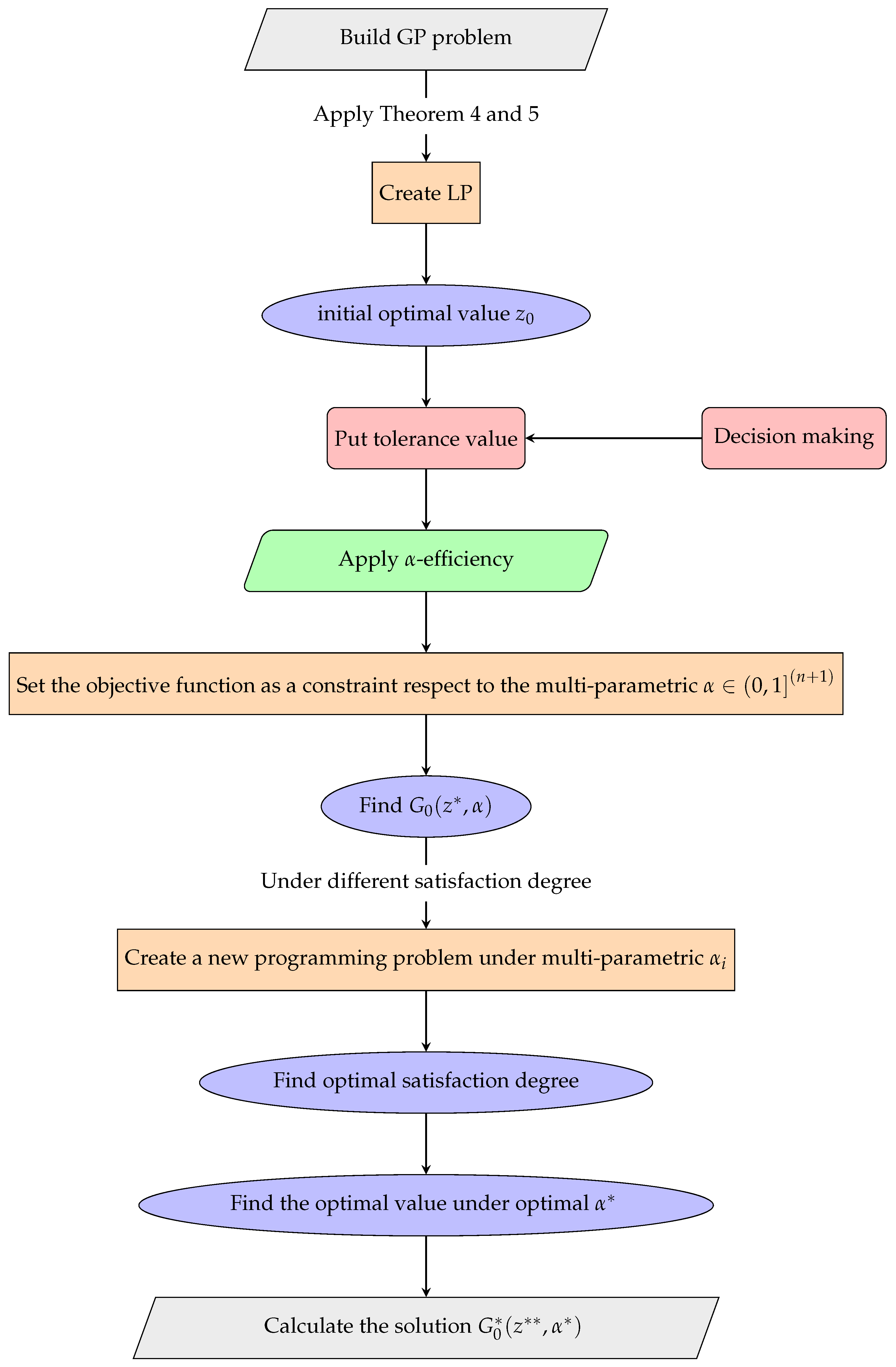
The method is depicted as a flowchart in Figure 1.

5. Comprehensive Analysis

Here, the proposed method and previous works are investigated, and the advantages of the proposed method is considered.

5.1. Shortcomings of the Existing Methods

There have been so many works on the topic of decision making in geometric programming problems. Several authors have introduced certain methods to find the optimal solution. In a like manner, we considered the methods that have been developed and proposed a new method for removing the shortcomings of the existing methods.

Up to now, the simple vector $\alpha$ was proposed, which was the same for all the constraints, and the expert person was forced to give the same satisfaction level to the decision maker for all constraints [31]. This creates a dilemma for the expert person, who is seeking the optimal solution and to satisfy the decision maker. Thus, for the sake of the importance of the optimal solution, the satisfaction level of the decision maker will rest on the second step. In our work, while we keep the optimal solution for fuzzy geometric programming, the satisfaction level of the decision maker is also provided.

In [20], multi-parametric programming is suggested to reach the optimal solution for a linear programming problem. The author proposed a vector to find a better satisfactory degree for the decision maker in a linear programming problem. In this method, an n-dimensional vector is introduced that does not actually approach the maximum satisfaction level for the decision maker and is not on fuzzy numbers. As we can see, most of the mathematical models in the real world are geometric programming models, and consequently, the demand for the decision maker has been applied to the geometric programming form, so we need to proposed a multi-parametric vector that can reach an optimal solution on geometric programming under the maximum satisfaction level of the decision maker.

5.2. The Advantages of the Proposed Method

It is shown that by using the proposed method, all of the shortcomings in existing methods can be avoided. Moreover, it is better to use this method for solving such problems, which occur in real life situations, as compared to the existing methods. By using the proposed algorithm to find the maximum satisfaction degree of the decision maker with the optimal solution of the fuzzy geometric programming problem, we have the following advantages:

(1)

Our work is on a geometric programming problem.

(2)

This method is proposed on fuzzy numbers.

(3)

The objective function is changed into the constraint. Thus, the solution starts with the initial optimal value.

(4)

One constraint is added to the constraints of the fuzzy geometric programming problem, which creates one more dimension and one more restriction on the feasible solution region. Thus, the proposed multi-parametric vector has $(n+1)$ dimensions.

(5)

This method gives more flexibility to the decision maker to put his desire on each constraint distinctively.

(6)

The decision maker’s order can also be put on the objective function when we deal with this as a constraint.

(7)

Creating a precise fuzzy geometric programming problem under a decision making tolerance value.

(8)

Satisfying the decision maker’s maximum desire.

(9)

The suggested approach in this study is applied and utilized.

6. Illustration of the Superiority of the Proposed Method

In this section, an instance of the fuzzy geometric programming problem to illustrate the proposed method is given. First, we solve the example with the multi-parametric vector $\alpha$ and then express the superiority of the multi-parametric vector $\alpha$ over the one-dimensional vector $\alpha$.

Example 1.

A septic productive factory produces concrete pipes for its projects. This factory needs to produce utmost $e^{19},e^{46}$, and $e^{64}$ (kg) of three types of concrete pipes $A_1$, $A_2$, and $A_3$, respectively. The pipes have to be produced by using four different kinds of concrete $B_1$, $B_2$, $B_3$, and $B_4$. The percentage of each type of raw concrete needed in each pipe (kg) and its unit price ($/kg) are listed in

Table 1. The percentage of concrete and its unit price.

	${\mathit{B}}_1$	${\mathit{B}}_2$	${\mathit{B}}_3$	${\mathit{B}}_4$	Required (kg)
$A_1$	(0,1,1,2)	(0,1,3,4)	(1,1,1,1)	(1,2,2,3)	$e^{19}$
$A_2$	(5,6,6,7)	(3,4,6,7)	(2,3,3,4)	(0,2,2,4)	$e^{46}$
$A_3$	(1,2,4,5)	(2,3,5,6)	(1,1,3,3)	(10,11,13,14)	$e^{64}$
unit price ($/kg)	5	6	3	5

. Find the maximum raw concrete needed under the owner’s tolerance level.

Solution. This problem can be induced in the fuzzy form of a PGP problem as follows:

$$\tilde{\max }{x_1}^5{x_2}^6{x_3}^3{x_4}^5$$

(18)

$$s.t.{x_1}^{(0,1,1,2)}{x_2}^{(0,1,3,4)}{x_3}^{(1,1,1,1)}{x_4}^{(1,2,2,3)},⩽e^{19}$$

$${x_1}^{(5,6,6,7)}{x_2}^{(3,4,6,7)}{x_3}^{(2,3,3,4)}{x_4}^{(0,2,2,4)},⩽e^{46},$$

$${x_1}^{(1,2,4,5)}{x_2}^{(2,3,5,6)}{x_3}^{(1,1,3,3)}{x_4}^{(10,11,13,14)},⩽e^{64},$$

$$x_1,x_2,x_3,x_4>0.$$

Here, we perform the steps of the method as expressed above.

Due to the definition of the membership function, for constraints and the objective function, we have the following membership functions, respectively:

$${\mu }_i(A_{i}x,B_i)=\left\{\begin{array}{cc}1,\hfill & G_i(z,{\alpha }_i)⩽B_i,\hfill \\ \frac{B_i+q_i-G_i(z,{\alpha }_i)}{q_i},\hfill & B_i⩽G_i(z,{\alpha }_i)⩽B_i+q_i,i=1,2,3,\hfill \\ 0,\hfill & G_i(z,{\alpha }_i)⩾B_i+q_i,\hfill \end{array}\right.$$

(19)

$${\mu }_0\left(G_0(z,{\alpha }_0)\right)=\frac{z_0-G_0(z,{\alpha }_0)}{q_0},z_0-q_0⩽G_0(z,{\alpha }_0)⩽z_0.$$

(20)

Utilize $x_j=e^{z_j}$, $(1⩽j⩽4)$. Problem (18) is changed into the following fuzzy problem under Theorems 3 and 4:

$$\tilde{\max }5z_1+6z_2+3z_3+5z_4$$

(21)

$$s.t.(0,1,1,2)z_1+(0,1,3,4)z_2+(1,1,1,1)z_3+(1,2,2,3)z_4⩽19$$

$$(5,6,6,7)z_1+(3,4,6,7)z_2+(2,3,3,4)z_3+(0,2,2,4)z_4⩽46,$$

$$(1,2,4,5)z_1+(2,3,5,6)z_2+(1,1,3,3)z_3+(10,11,13,14)z_4⩽64,$$

The first step is to apply the ranking function on trapezoidal fuzzy numbers under the Remark 3.

$$\tilde{\max }5z_1+6z_2+3z_3+5z_4$$

(22)

$$s.t.z_1+2z_2+z_3+2z_4⩽19,$$

$$6z_1+5z_2+3z_3+2z_4⩽46,$$

$$3z_1+4z_2+2x_3+12z_4⩽64.$$

The initial optimal solution is taken from the basic variables as $x_1=e^{2.12}$, $x_2=e^{5.45},x_3=1$, $x_4=e^{2.98}$, and the optimal value equals $e^{58.27}$.

From the first step, by applying $x_0=e^{z_0}$, we find $z_0=58.27$.

According to the two-phase method, we can change problem (22) into the following programming problem:

$$\tilde{\max }5z_1+6z_2+3z_3+5z_4$$

(23)

$$s.t.K_0(z,{\alpha }_0)=5z_1+6z_2+3z_3+5z_4⩾z_0-{\alpha }_0{q}_0,$$

$$z_1+2z_2+z_3+2z_4⩽19+(1-{\alpha }_1)q_1,$$

$$6z_1+5z_2+3z_3+2z_4⩽46+(1-{\alpha }_2)q_2,$$

$$3z_1+4z_2+2x_3+12z_4⩽64+(1-{\alpha }_3)q_3,$$

$${\alpha }_i\in (0,1],i=0,1,2,3.$$

Suppose that $q_0=5,q_1=1,q_2=4$, and $q_3=6$ are the maximum toleration values for $q_i,(i=0,1,2,3)$, which is given by decision maker, then substitute $z_0,q_0,q_1,q_2$ and $q_3$ into problem (23). We have:

$$\tilde{\max }5z_1+6z_2+3z_3+5z_4$$

(24)

$$s.t.5z_1+6z_2+3z_3+5z_4+5{\alpha }_0⩾58.27,$$

$$z_1+2z_2+z_3+2z_4+{\alpha }_1⩽20,$$

$$6z_1+5z_2+3z_3+2z_4+4{\alpha }_2⩽50,$$

$$3z_1+4z_2+2x_3+12z_4+6{\alpha }_3⩽70,$$

$${\alpha }_i\in (0,1],i=0,1,2,3.$$

Table 2. Finding the maximum satisfaction degree with a multi-parametric $\alpha$.

	1	2	3	4	5
$\alpha$	(0.5,0.5,0.5,0.5)	(0.5,0.8,0.5,0.5)	(0.8,0.5,0.8,0.5)	(0.9,0.5,0.5,0.7)	(0.9,0.8,0.8,0.7)
$z_1$	2.51	2.76	2.2	2.4	2.34
$z_2$	5.3	4.98	5.42	5.5	5.29
$z_3$	0	0	0	0	0
$z_4$	3.18	3.22	3.22	3.05	3.13
$K_0(z,{\alpha }_i)$	60.34	59.9	59.68	60.25	59.15

shows the decision maker’s satisfaction at different $\alpha$-efficiency confidence levels. If $\alpha =({\alpha }_0,{\alpha }_1,{\alpha }_2,{\alpha }_3)$ and $G_0(z^{*},\alpha )$ denote the optimal value of the objective function at each step under different $\alpha$s, we can have the table as follows, which is procured by the MATLAB software:

The values observed in Table 2 demonstrates that ${\alpha }_1$ and ${\alpha }_2$ are the most inefficient components. From columns 2, 3, and 5 in Table 2, it can be deduced that by increasing ${\alpha }_1$ and ${\alpha }_2$, the optimal solution will be strayed away. Reducing ${\alpha }_1$ and ${\alpha }_2$ achieves a better result. Again from columns 1 and 4 in Table 2, one can get closer to the optimal solution by increasing ${\alpha }_0$ and ${\alpha }_3$. Now from here, we will try to minimize ${\alpha }_1$ and ${\alpha }_3$ by choosing the $(0.5,0.5,0.5,0.5)$-efficient solution with optimal value $G_0(z^{*},\alpha )=60.34$ as an initial solution.

Figure out the LP problem below affected by $G_0(z^{*},\alpha )=60.34$:

$$\max {\alpha }_0+{\alpha }_1+{\alpha }_2+{\alpha }_3$$

(25)

$$s.t.5z_1+6z_2+3z_3+5z_4+5{\alpha }_0⩾60.34,$$

$$z_1+2z_2+z_3+2z_4+{\alpha }_1⩽20,$$

$$6z_1+5z_2+3z_3+2z_4+4{\alpha }_2⩽50,$$

$$3z_1+4z_2+2x_3+12z_4+6{\alpha }_3⩽70,$$

$$0.5⩽{\alpha }_0⩽1,$$

$$0.5⩽{\alpha }_1⩽1,$$

$$0.5⩽{\alpha }_2⩽1,$$

$$0.5⩽{\alpha }_3⩽1.$$

By maximizing the satisfaction degree, the optimal solution of problem (25) will be obtained as $z^{**}=(2.51,5.3,0,3.18)$ under the confidence level ${\alpha }^{*}=(1,0.5,0.5,0.5)$ and the optimal value computed with respect to ${\alpha }^{*}$ as $G_0^{*}(z^{**},{\alpha }^{*})=(2.51,5.3,0,3.18,1,0.5,0.5,0.5)=60.34$. Subsequently, the optimal solution for GP programming problem (18) will be $x_1=e^{2.51}$, $x_2=e^{5.3},x_3=1$, $x_4=e^{3.18}$, and the optimal value will be equal to $e^{60.34}$.

To compare this GP problem when the vector $\alpha$ is not multi-parametric, see

Table 3. Finding the maximum satisfaction degree with $\alpha$.

	1	2	3	4	5
$\alpha$	0.5	0.6	0.8	0.9	1
$z_1$	2.51	2.43	2.28	2.2	2.12
$z_2$	5.3	5.33	5.39	5.42	5.45
$z_3$	0	0	0	0	0
$z_4$	3.18	3.14	3.06	3.02	2.98
$K_0(z,{\alpha }_i)$	60.34	59.93	59.1	58.68	58.27

.

A comparison of Table 2 and Table 3 reveals that in Table 3, by increasing the confidence level $\alpha$, the optimal solution is minimized, whereas we expect to maximize the optimal solution when the confidence level rises. Indeed, the satisfaction degree for each constraint should be increased or decreased by the same amount, while in the proposed method, there is a chance to decrease or increase the satisfaction level for each constraint separately. In addition, an opportunity lies in dedicating a satisfaction level to the objective function. In Table 3, it is obvious that by increasing the confidence level, we get opposite results for the optimization, and the optimal value goes to its normal optimal solution, while in Table 2 the optimal value is kept optimal, as long as the satisfaction degree components are changing. The reason is that the vector $\alpha$ is not appropriate for all constraints, and particularly with turning the objective function to the constraint. In Table 3, $\alpha =0.5\in (0,1]$ can be noted as $\alpha =(0.5,0.5,0.5,0.5)\in {(0,1]}^4$ for $\alpha =({\alpha }_0,{\alpha }_1,{\alpha }_2,{\alpha }_3)$, whereas in Table 2, the satisfaction degree is $\alpha =(1,0.5,0.5,0.5)$. This implies that the one-dimensional satisfaction degree is meaningless in this case. It is clear that the flexibility of the $(n+1)-$dimensional confidence level ${\alpha }_i$ can help to reach a better optimal solution that implements decision maker’s goal.

7. Conclusions

In this paper, a new insight to the satisfaction degree is introduced. The multi-parametric vector $\alpha$ is gained under the tolerance value of the decision maker’s order and increases the likelihood of obtaining the highest satisfaction level. This method helps us solve the fuzzy geometric programming problem by coming up with an optimal solution that satisfies the decision maker. This method does not force the decision maker to choose the same tolerance value for all constraints. The expert person can satisfy the decision maker in each constraint distinctively under the optimal value of the fuzzy geometric programming problem. Moreover, by converting the objective function in the initial programming problem to the constraint in the reversed geometric programming problem, we can obtain the best optimal solution under the decision maker’s maximum desire. By comparing Table 2 and Table 3, it can be deduced that in Table 3, using a one-dimensional $\alpha$ to determine the satisfaction degree for all constraints and the objective function led to an inverse result. But in Table 2, utilizing a multi-parametric $\alpha$ that is assigned to every constraint distinctively assists us in obtaining a better satisfaction degree. It is evident from Table 2 that the full satisfaction degree is achieved for the first component of $\alpha$ under the decision maker’s tolerance level; however, in the current method, getting full satisfaction for one of the constraints is impossible. In addition, applying the satisfaction degree on the objective function is an efficient approach to obtain the best optimal value. In future work, fuzzy numbers with negative elements will be considered, which has applications in cost and benefit problems. A subsequent paper will focus on multi-criteria decision making, which includes both costs and benefits. Thus, the proposed method can be used in economics and industrial problems.

References

- Fu, S.; Wen, H.; Wu, B. Power-fractionizing mechanism: Achieving joint user scheduling and power allocation via geometric programming. IEEE Trans. Veh. Technol. 2018, 67, 2025–2034. [Google Scholar] [CrossRef]
- Li, Z.; Vatankhah, A.; Jiang, J.Y.; Zhong, R.; Xu, G. A mechanism for scheduling multi robot intelligent warehouse system face with dynamic demand. J. Intell. Manuf. 2018, 1–12. [Google Scholar] [CrossRef]
- Rajeswari, P.; Shekar, G.; Devi, S.; Purushothaman, A. Geometric Programming-Based Power Optimization and Design Automation for a Digitally Controlled Pulse Width Modulator. Circuits Syst. Signal Process. 2018, 37, 4049–4064. [Google Scholar] [CrossRef]
- Dantzig, G. Linear Programming and Extensions; Princeton University Press: Princeton, NJ, USA, 2016. [Google Scholar]
- Boyd, S.; Kim, S.J.; Vandenberghe, L.; Hassibi, A. A tutorial on geometric programming. Optim. Eng. 2007, 8, 67–127. [Google Scholar] [CrossRef]
- Zadeh, L.A. Fuzzy sets. Inf. Control 1965, 8, 338–353. [Google Scholar] [CrossRef] [Green Version]
- Tanaka, H.; Okuda, T.; Asai, K. On fuzzy mathematical programming. J. Cybernet 1974, 3, 37–46. [Google Scholar] [CrossRef]
- Zimmermann, H.J. Fuzzy programming and linear programming with several objective functions. Fuzzy Sets Syst. 1978, 1, 45–55. [Google Scholar] [CrossRef]
- Ostrosi, E.; Haxhiaj, L.; Fukuda, S. Fuzzy modelling of consensus during design conflict resolution. Res. Eng. Des. 2012, 23, 53–70. [Google Scholar] [CrossRef]
- Ezzati, R.; Khorram, E.; Enayati, R. A new algorithm to solve fully fuzzy linear programming problems using the MOLP problem. Appl. Math. Model. 2015, 12, 3183–3193. [Google Scholar] [CrossRef]
- Inearat, L.; Qatanani, N. Numerical methods for solving fuzzy linear systems. Mathematics 2018, 6, 19. [Google Scholar] [CrossRef]
- Pishvaee, M.S.; Khalaf, M.F. Novel robust fuzzy mathematical programming methods. Appl. Math. Model. 2016, 40, 407–418. [Google Scholar] [CrossRef]
- Garg, H. Non-linear programming method for multi-criteria decision making problems under interval neutrosophic set environment. Appl. Intell. 2018, 48, 2199–2213. [Google Scholar] [CrossRef]
- Bellman, R.E.; Zadeh, L.A. Decision making in a fuzzy environment. Manag. Sci. 1970, 17, 141–164. [Google Scholar] [CrossRef]
- Joshi, D.K.; Beg, I.; Kumar, S. Hesitant probabilistic fuzzy linguistic sets with applications in multi-criteria group decision making problems. Mathematics 2018, 6, 47. [Google Scholar] [CrossRef]
- Naz, S.; Ashraf, S.; Akram, M. A novel approach to decision-making with Pythagorean fuzzy information. Mathematics 2018, 6, 95. [Google Scholar] [CrossRef]
- Faísca, N.P.; Saraiva, P.M.; Rustem, B.; Pistikopoulos, E.N. A multi-parametric programming approach for multilevel hierarchical and decentralised optimization problems. Comput. Manag. Sci. 2007, 6, 377–397. [Google Scholar] [CrossRef]
- Liou, T.S.; Wang, M.J.J. Ranking fuzzy numbers with integral value. Fuzzy Sets Syst. 1992, 50, 247–255. [Google Scholar] [CrossRef]
- Hernandes, F.; Lamata, M.T.; Verdegay, J.L.; Yamakami, A. The shortest path problem on networks with fuzzy parameters. Fuzzy Sets Syst. 2007, 14, 1561–1570. [Google Scholar] [CrossRef]
- Attari, H.; Nasseri, S.H. New Concepts of Feasibility and Efficiency of Solutions in Fuzzy Mathematical Programming Problems. Fuzzy Inf. Eng. 2014, 6, 203–221. [Google Scholar] [CrossRef] [Green Version]
- Cao, B.Y. Solution and theory of question for a kind of fuzzy positive geometric program. In Proceedings of the 2nd IFSA Congress, Tokyo, Japan, 20–25 July 1987. [Google Scholar]
- Mendel, J.M. Type-2 fuzzy sets. In Uncertain Rule-Based Fuzzy Systems; Springer: Cham, Swizerlands, 2017; pp. 259–306. [Google Scholar]
- Wu, H.C. On interval-valued nonlinear programming problems. J. Math. Anal. Appl. 2008, 338, 299–316. [Google Scholar] [CrossRef] [Green Version]
- Khastan, A.; Perfilieva, I.; Alijani, Z. A new fuzzy approximation method to Cauchy problems by fuzzy transform. Fuzzy Sets Syst. 2016, 288, 75–95. [Google Scholar] [CrossRef]
- Jafarian, E.; Razmi, J.; Baki, M.F. A flexible programming approach based on intuitionistic fuzzy optimization and geometric programming for solving multi-objective nonlinear programming problems. Expert Syst. Appl. 2018, 93, 245–256. [Google Scholar] [CrossRef]
- Ruan, G.Z.; Wang, S.Y.; Yamamoto, Y.; Zhu, S.S. Optimality conditions and geometric properties of a linear multilevel programming problem with dominated objective functions. J. Optim. Theory Appl. 2004, 123, 409–429. [Google Scholar] [CrossRef]
- Lai, Y.J. Hierarchical optimization: A satisfactory solution. Fuzzy Sets Syst. 1996, 77, 321–335. [Google Scholar] [CrossRef]
- Shih, H.S.; Lai, Y.J.; Lee, E.S. Fuzzy approach for multi-level programming problems. Comput. Oper. Res. 1996, 23, 73–91. [Google Scholar] [CrossRef]
- Sakawa, M.; Nishizaki, I.; Uemura, Y. Interactive fuzzy programming for multilevel linear programming problems. Comput. Math. Appl. 1998, 36, 71–86. [Google Scholar] [CrossRef] [Green Version]
- Chong, E.K.P.; Zak, S.H. An Introduction to Optimization; John Wiley & Sons; Inc.: New York, NY, USA, 1996. [Google Scholar]
- Cao, B.Y. Optimal Models and Methods with Fuzzy Quantities; Springer: Berlin/Heidelberg, Germany, 2010. [Google Scholar]
- Dubois, D.; Prade, H. Operations on fuzzy numbers. Int. J. Syst. Sci. 1978, 9, 613–626. [Google Scholar] [CrossRef]
- Cao, B.Y. Fuzzy geometric programming (I). Fuzzy Sets Syst. 1993, 53, 135–153. [Google Scholar]
- Bazaraa, M.S.; Sherali, H.D.; Shetty, C.M. Nonlinear Programming: Theory and Algorithms; John Wiley & Sons: Hoboken, NJ, USA, 2013. [Google Scholar]
- Wang, X.; Kerre, E.E. Reasonable properties for the ordering of fuzzy quantities (II). Fuzzy Sets Syst. 2001, 118, 387–405. [Google Scholar] [CrossRef]
Figure 1.
A flowchart for our method.