Constrained FC 4D MITPs for Damageable Substitutable and Complementary Items in Rough Environments
by
 , ,
, ,
Sharmistha Halder Jana
1,* ,
,
Biswapati Jana
2,
Barun Das
3,
Goutam Panigrahi
4 and
Manoranjan Maiti
5 1
Department of Mathematics, Midnapore College (Autonomous), Midnapore 721101, India
2
Department of Computer Science, Vidyasagar University, Midnapore 721102, India
3
Department of Mathematics, Sidho Kanho Birsha University, Purulia 723104, India
4
Department of Mathematics, National Institute of Technology, Durgapur 713209, India
5
Department of Mathematics, Vidyasagar University, Midnapore 721102, India
*
Author to whom correspondence should be addressed.
Mathematics 2019, 7(3), 281; https://doi.org/10.3390/math7030281
Submission received: 2 January 2019
/
Revised: 25 February 2019
/
Accepted: 27 February 2019
/
Published: 19 March 2019
(This article belongs to the Special Issue Application of Optimization in Production, Logistics, Inventory, Supply Chain Management and Block Chain)
Abstract
:Very often items that are substitutable and complementary to each other are sent from suppliers to retailers for business. In this paper, for these types of items, fixed charge (FC) four-dimensional (4D) multi-item transportation problems (MITPs) are formulated with both space and budget constraints under crisp and rough environments. These items are damageable/breakable. The rates of damageability of the items depend on the quantity transported and the distance of travel i.e., path. A fixed charge is applied to each of the routes (independent of items). There are some depots/warehouses (origins) from which the items are transported to the sales counters (destinations) through different conveyances and routes. In proposed FC 4D-MITP models, per unit selling prices, per unit purchasing prices, per unit transportation expenditures, fixed charges, availabilities at the sources, demands at the destinations, conveyance capacities, total available space and budget are expressed by rough intervals, where the transported items are substitutable and complementary in nature. In this business, the demands for the items at the destinations are directly related to their substitutability and complementary natures and prices. The suggested rough model is converted into a deterministic one using lower and upper approximation intervals following Hamzehee et al. as well as Expected Value Techniques. The converted model is optimized through the Generalized Reduced Gradient (GRG) techniques using LINGO 14 software. Finally, numerical examples are presented to illustrate the preciseness of the proposed model. As particular cases, different models such as 2D, 3D FCMITPs for two substitute items, one item with its complement and two non substitute non complementary items are derived and results are presented.
1. Introduction
Due to globalization, nowadays, transportation of commodities from sources to the destinations by road is getting more important. The advent of transportation problem (TP) was mainly based on real-life problems. Many numbers of real-life goods carrying problems are easily framed as transportation problems. The credit of first transportation problem goes to Hitchcock [1], which is a particular case of Linear Programming Problem (LPP). This optimizing problem consists of two main constraints i.e., source and destination constraints. However, it is very common knowledge that, in practical situations, these two constraints are not enough to formulate the problem perfectly since there exist other constraints, namely mode of transport, type of products, the distance of path traveled, etc. Due to the presence of these additional real-life constraints, the conventional transportation problems (2D-TPs) are modified to a solid transportation problem (STP-3D-TPs), which was first developed by Schell [2]. After the advent of STP, it has swiftly gained a very important place for research and development in transportation. Researchers like Yang et al. [3], Kocken et al. [4], etc. were on the development of STP, in which conveyances at different sources are considered.
In general circumstances, the length of a route remains unchanged in a normal transportation problem, so it does not make any significant change in the minimization of cost or time. However, reality dictates that there may be a number of available option/paths for the transportation of an item from source to destination. The common knowledge suggests that the cost per unit for transportation or other fixed charges related to routes are of different values. Thus, it can be seen that a three-dimensional transportation problem (3D-TP) is converted to a 4D-TP. Such a 4D-TP was considered by Halder et al. [5].
Nowadays, the business of multi -items is quite popular. Normally, in business, it is thought that if one item brings loss, another item may produce the profit. Moreover, due to the constantly changing business environment, the parameters related to transportation are imprecise. This situation has been recently dealt with in two recent investigations Das et al. [6] and Bera et al. [7]. Again, the transportation of multi-items may be substitutable and/or complementary because more options/choices of items bring more customers. This is true for supply chain models. Recently, Sarkar and Lee [8] and sarkar et al. [9] presented optimum pricing strategies for complementary products using game the orectic approach. Khanna et al. [10] suggested supply chain with customer-based two-level credit policies under an imperfect quality environment. Recently, Halder et al. [5] also solved an FCSTP for substitute and breakable items in crisp and fuzzy environments.
1.1. Scope of the Paper
Considering the above facts, we formulate the transportation policies of some damageable substitute and/or complementary items from some sources to destinations using some convenient vehicles and appropriate routes where the parameters of the problem are deterministic or imprecise and some realistic resource constraints are imposed.
In this investigation, there are different types of conveyance at different sources and different routes/paths available to travel from a source to a destination. Along some paths, fixed charges such as toll taxes, festival collections, etc. are collected. At each destination, retailers have some limitations on space and budget. The transportation costs, fixed charges, availabilities, demands, resources are imprecise and expressed by rough intervals. As the items are substitutable and complementary, items’ demands are influenced by each other’s prices. The demand for an item is reduced due to its own and complementary item’s prices but increases due to its substitute’s price. With these features, the model is formulated as a constrained FC 4DMITP problem and solved using Generalised Reduced Gradient (GRG) method (using LINGO 14.0). As particular cases, transportation policies for several models (i.e., 2D, 3D TPs for different combinations of items) are derived. The model are illustrated numerically. Some sensitivity analyses are also performed. Results of an earlier investigation (Bera et al. [7]) are obtained as a particular case. The novelties of the present investigation are as follows:
- As earlier discussed, TP and STP with various types of constraints are considered by several researchers. However, few researchers have considered 4D-TPs and 4D-MITPs. Moreover, 4D-MITP with rough parameters is an updated contribution.
- The items are complementary and substitutable in nature, that is, demands of the items are appropriately affected by their selling prices.
- The most important issues of this paper are to analyze how the travel distances are related to profit maximization when manufacturing companies transport both complementary and substitute items that are differentiated by distance including the fixed charge of the path and damageability. The importance of route on profit is illustrated.
- Until now, in transportation, no one has considered the space constraint at the destinations along with the budget constant. The idea of space constraint is introduced here.
- The earlier researchers gave attention to minimization of aggregate transportation expenditure and very few have realized the importance of consideration of total profit instead of total cost/expanses.
- As particular cases, several earlier transportation models are deduced from the present model.
1.2. Structure of the Paper
The structure/organization of the paper is split as:
- Section 1: Introduction
- Section 2: Notations and Assumptions for the proposed model are given.
- Section 3: Model description and formulation
- Section 4: Numerical Experiments
- Section 5: Particular Cases
- Section 6: Sensitivity Analyses
- Section 7: A discussion of the models on the basis of numerical results are presented.
- Section 8: Practical implication is described.
- Section 9: Conclusions drawn.
1.3. Literature Review
Though the transportation problem is quite an age-old one, several researchers are still working in this area as it is important due to national highways within the country and international transportation using cargos and ships. Hirsch and Dantzig [11] first introduced the concept of a fixed charge transportation problem in 1968. In each country, there are different major highways connecting the cities/ports and, for the maintenance, some charges (fixed) are collected from the vehicles plying on these roads. This real-life scenery has been depicted in the fixed charge TPs (FCTP). Kowalski and Lev [12] developed the FCTP as a nonlinear programming problem of practical interest in business and industry. Gen et al. [13] discussed the bi-criteria solid transportation problem with equality constraints solved by a genetic algorithm. Several researchers like Verma et al. [14], Shafaat and Goyal [15], Saad and Abbas [16] and others worked on transportation problems.
Though there are a lot of works on damageable/deteriorating items in inventory (cf. Sarkar and Iqbal [17] and Sarkar et al. [18]), only limited works have been done on damageable/breakable items in transportation. This is because transportation time is not normally considered in TP. However, the damageability may also depend on the route lengths which are different for different routes. Pramanik et al. [19] presented a multi-objective solid transportation problem with reliability for damageable items in a random-fuzzy environment.
Though Sarkar et al. [20] considered a power function of the delivery quantity as a unit transportation cost in inventory, normally constant unit transportation cost is assumed in TP to formulate it as an LPP. Ojha et al. [21] presented a solid transportation problem with nonlinear transportation cost and fuzzy resources, demand and conveyances. However, in the present problem, transportation cost is considered constant. Depending on different aspects, unit transportation costs, resources, demands, available budget and storing capacity at destination, etc. fluctuate due to uncertainty in judgement, lack of evidence, insufficient information, etc. Thus, a transportation model becomes more realistic if these parameters are assumed to be flexible /imprecise in nature i.e., uncertain in non-stochastic sense which may be represented by fuzzy, rough [22], type-2-fuzzy, fuzzy stochastic numbers. There are several investigations on TPs with fuzzy parameters. Verma et al. [14], Bit et al. [23], Jimenez and Verdegay [24], Li and Lai [25], Dey et al. [26] and others solved fuzzy multi-objective TP(s) using a Fuzzy compromise programming approach. Yang and Liu [3] investigated a fixed charge STP with fuzzy costs, fuzzy supplies, fuzzy demands and fuzzy conveyance capacities using an expected value method. There are also many investigations on TP with rough parameters. Recently, Kundu et al. [27] presented an STP considering crisp and rough costs. Tao et al. [28] applied rough multiple objective programming in STP. Das et al. [6] developed a profit-maximizing STP with parameters represented by rough intervals. Recently, Bera et al. [7] solved multi-item 4D TPs under budget constraints using rough interval values for TP parameters. The year-wise investigations of various TPs and STPs with different variations are recorded in the following table.
In spite of all these investigations, there are still some lacunas in making the investigated problem more realistic ones. Some of these gaps such as substitutable and complementary items, both budget and space constraint, damageable units, 4D MITP, fixed charge, profit maximization, etc. have been taken into account in the present investigation.
1.4. Motivation
Although there are so many existing kinds of literature available in the field of transportation problem (cf in Table 1), but still there are some lacunas. Most of the researchers developed two-dimensional or three-dimensional problems that motivated us to form a four-dimensional real transportation problem.
In modern business, multifarious items are preferable for transportation rather than the single item. In the long term, transportation system fixed charges like (road tax etc.) are very common to real life; this is also a motivation which leads to consideration of fixed charge. Finally, in today’s constantly fluctuating life, uncertainty is the only certain factor in our life. In this concept, the different coefficients are not fixed to its deterministic values. It must take an interval. For example, demand of an item is not fixed, but it is represented by its lower and upper limits , , respectively. Again, this limit also may fluctuate, so the necessity of rough interval arise. In this regard, the demand for an item roughly lies on , respectively.
In reality, most of the problems are not described specifically but described with uncertainty. This may due to the fluctuation of daily life, lack of information, etc. Until now, most of the impreciseness are described by interval values.
In interval analysis, a parameter is represented by lower and upper limits and the possibility of existence of every point within this limits are same. However, in reality, it is not so, where the lower ‘a’ and upper limits ‘b’ occurred very occasionally. Most of the time, there exists a normal interval , where . Thus, vagueness here is described by two nested intervals . Such representation is well known as a rough interval.
For example, if we go through “Air Quality Index (AQI)” measurement of the city Ananda Vihar, Delhi in the year 2017, the lower and the upper intervals of this AQI (measured by PM2.5) were . The AQI 78 g/m found in the day of July 2017 (during rainy season) and the AQI is 404 g/m is found on the day of Dewali (November 2017), whereas the normal range of AQI (PM2.5) is [150, 290]. In this regard, the rough representation of AQI (PM2.5) of Ananda Vihar New Delhi is ([78, 404], [150, 290]).
2. Notation and Assumptions
2.1. Notations
2.1.1. Parameters
For r-th item,
- : quantity of homogeneous merchandise available at i-th source.
- : market demand at j-th goal.
- : actual demand at j-th goal.
- : quantity of the merchandise which can be carried by k-th conveyance along p-th route.
- : per unit transportation price from i-th origin to j-th goal by k-th vehicle via p-th route.
- : selling expenses at the j-th destination.
- : purchasing price at the i-th origin.
- : fixed transportation cost for shipping units from i-th source/origin to j-th goal/destination by k-th vehicles along p-th route.
- : rate of breakability per unit distance from i-th source to j-th goal via p-th route and k-th conveyance.
- : total budget at the j-th goal point.
- : distance from i-th origin to j-th goal along p-th route.
- : required space for r-th item.
- : available space to the j-th retailer.
- : power of the route length, related with the frangibility.
- , , and : Price sensitivity of products.
2.1.2. Decision Variable
- : the transported quantity from i-th source/origin to j-th goal/destination by k-th vehicle along p-th route (decision variable).
2.1.3. Indices
- R: total number of items.
- M: total number of origin/sources.
- N: total number of goal/destinations.
- L: total number of route/paths.
- K: total number of vehicles/conveyance.
2.2. Assumptions
- (i)
- Particulars are breakable and carried from sources to goals using a vehicle through a path. Broken/damaged amounts depend on conveyance and path.
- (ii)
- Particulars are substitutable and complementary to each other. In case of a substitute item, the demand is negative and is positive when the items are complementary nature:
3. Model Description and Formulation
Let us define a four-dimensional transportation problem in this way. A merchant/wholesaler having different M godowns/storing houses (sources) at different locations and different N sales counters/shops (destinations) in different cities. The merchant buys R number of items of which some are substitutes and others complementary to each other and stores at the godowns which are of finite capacities. There are different K conveyances and L routes for transportation of goods from sources to destinations.
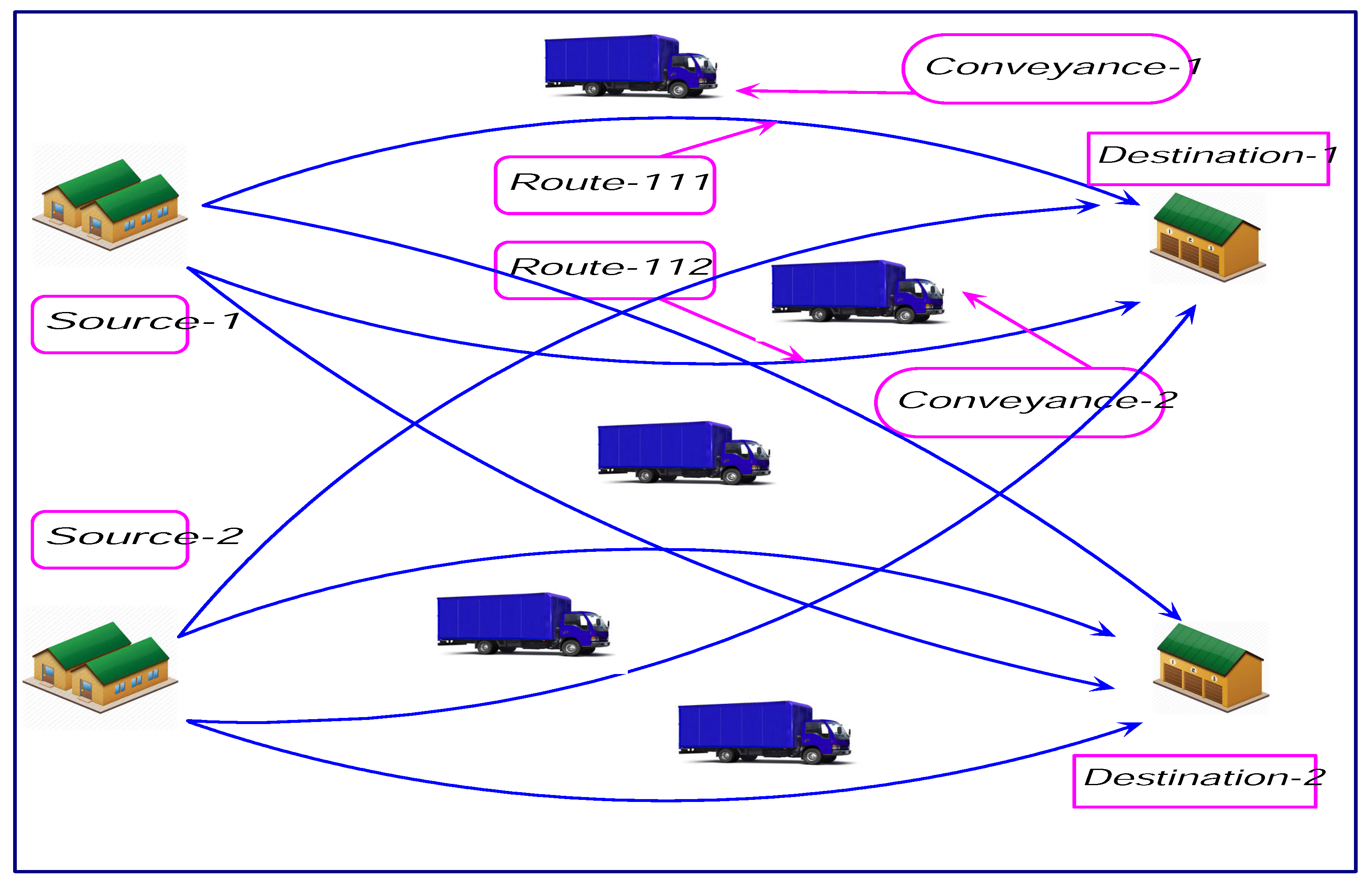
The schematic diagram of this 4D-MITP is given in Figure 1. The conveyances are of finite capacities and charge different charges for transportation along different routes. There are some fixed costs/charges (toll taxes, etc.) along each route and items are damageable. This damageability depends on type of conveyance and the distance of traveled by that conveyance. At each destination, the items are known and, for that, some amount of items are stored as per the capacities of the go-downs. The merchant can use any conveyance and route for transportation and the above mentioned transportation parameters are crisp or rough interval numbers. At the destination, the merchant sells the good items at some prices. The merchant has a limitation on his initial expenditure. Now, the problem for the merchant is to decide the amount of quantities to be transported from different sources to different destinations by the appropriate conveyance through the appropriate route so that total profit out of this business is at a maximum subject to the constraints.
Thus, TP is developed as a profit maximization problem. In this process of business, there are total purchase charge cost, fixed charge cost, transportation cost, revenue in the objective functions and five constraints on source, destination, conveyance capacity, space and budget. Therefore, as per the availability of type of the input parameters with the help of considerable assumptions and notations, we formulate two different models: the crisp model and rough model as given below.
3.1. Model-I: Crisp Model
3.2. Model-II: Rough Model
If the parameters, selling expenses, cost of transportation, purchasing prices, fixed charges, availability, demand, capacities, available space and permittable budget are found as rough intervals i.e.,
Thus, after the introduction of these rough parameters, the above crisp model (1) is translated to the following rough model:
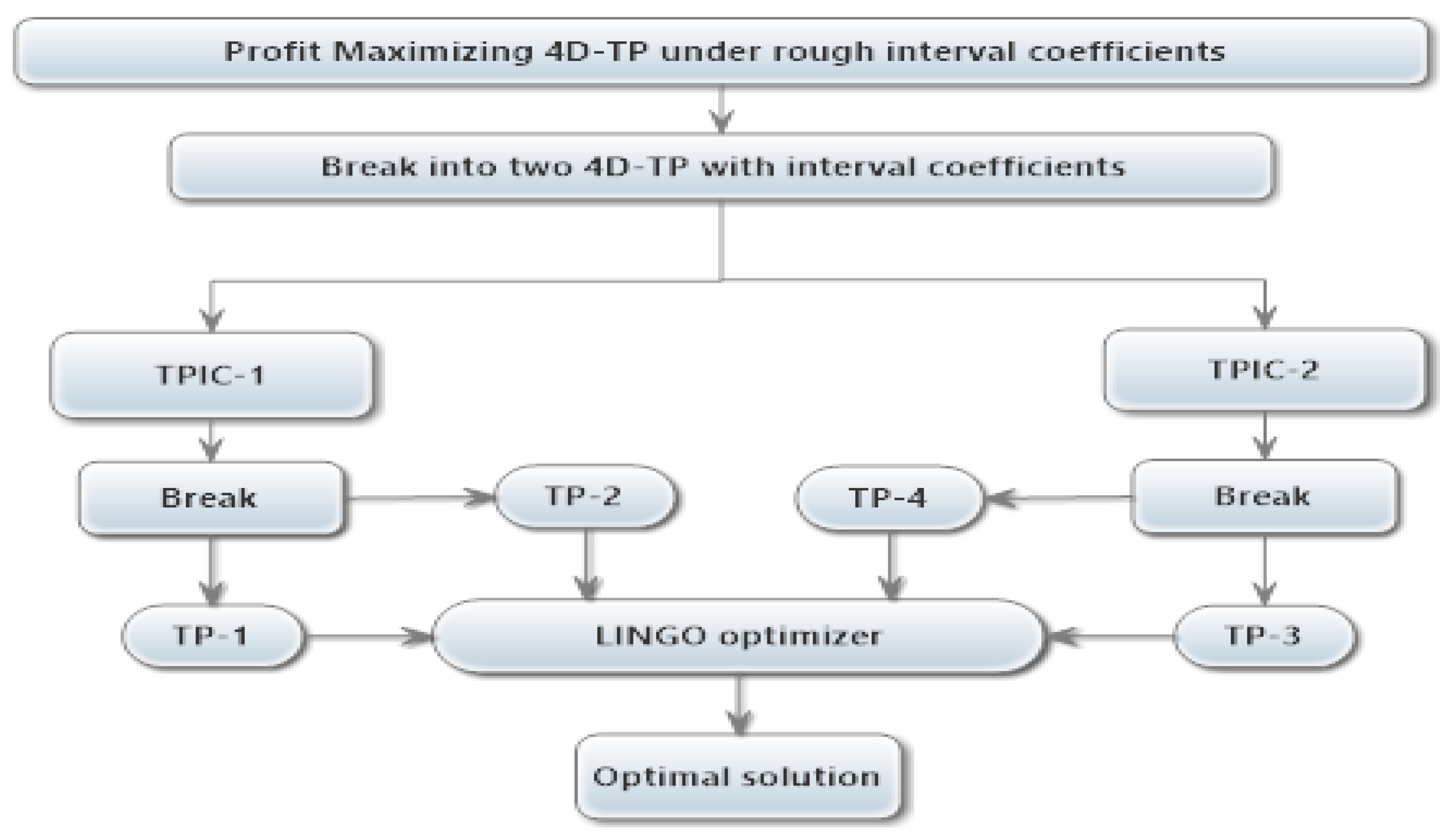
According to the discussion of Linear Programming issues with Rough Interval Coefficient (LPRIC) in Appendix A.1, at first, we get two different transportation problems (TPIC-1, TPIC-2) with interval coefficients—and again, as discussed, TPIC-1 and TPIC-2 broken as TP-1, TP-2 and TP-3, TP-4. The above stated consideration can be graphically represented in Figure 2.
3.3. The Mathematical Form of TPIC-1
3.4. The Mathematical Form of TPIC-2
3.4.1. TP-1
3.4.2. TP-2
3.4.3. TP-3
3.4.4. TP-4
3.4.5. Approach-2
After use of the Expected Value Method, the Rough transportation problem ( Model-II) mathematically reduces to:
The problem (16) can be written as:
4. Numerical Experiments
Let us consider a real life transportation system where number of sources = 2 (i.e., M = 2), number of destination = 2 (i.e., N = 2), number of vehicles = 2 (i.e., K = 2) and number of routes = 2 (L = 2), number of items = 3 (i.e., R = 3). The input values of unit transportation costs, fixed charges are of crisp and rough interval forms which are presented in Table 2 and Table 3. The amount of breakability in a crisp environment is also presented in Table 2. Here, it is assumed that there are three types of products. The 1st and 2nd ones are the substitute, the 1st and 3rd are complementary, and the 2nd and 3rd are also complimentary.
The other parametric magnitudes such as unit purchasing price and unit selling price, capacities of conveyances, available space, budget, sources and demands of the Models-I and -II are given in Table 3 and Table 4. Let the unit space for 1st, 2nd and 3rd items are two units, three units and two units.
By considering the general demand function, it is necessary to define , , and . These parameters are defined as follows: , , and . The following Table 5 represent the distances from different origins to destinations by route-1 and route-2.
Now, the problem is to determine the optimal policy of transportation to maximize the profit. Under the objective of maximization of profit subjected to the traditional constraints, available space, and budget constraints for the above given input data, the crisp model is solved using Generalised Reduced Gradient (GRG) method and rough model by (i) Hamzehee et al and (ii) Expected Value Techniques along with GRG method. The results are presented in Table 6 (Crisp Model and Rough Model by Hamzehee Method) and Table 7 (Rough Model by Expected Value Technique). The convergence of the GRG method is also well established (shown in Appendix A.5) [33].
To compare the results for existence of different constraints, we present the following Table 8 for = 0.5.
5. Particular Cases
5.1. Three-Dimensional TP Model
If we take the system where there is only one route only, i.e., L = 1 in the Model-II (Rough Model), then the converted transportation problem is termed as a solid transportation problem (STP). The corresponding three dimensional TP-1, TP-2, TP-3, TP-4 is obtained by substituting L = 1 in the TP-1, TP-2, TP-3, TP-4 of the four-dimensional transportation Model. The results of the 3DTP (i.e., STP) model are given in Table 9.
If we take K = 1, then we get another three-dimensional transportation Model. Like above, the corresponding 3D TP-1, TP-2, TP-3, TP-4 are found by substituting K = 1 in the TP-1, TP-2, TP-3, TP-4 of the four-dimensional transportation Model. The optimum results of this STP model are given in Table 10.
5.2. 2D-TP Model
If we take L = 1 and K = 1 in the Model-II (Rough Model), then we get the 2D-transportation problem. The corresponding 2D TP-1, TP-2, TP-3, TP-4 are found in the following Table 11.
5.3. 4D-TPs with Different Natures of the Items
Results for the different combinations of substitute and complementary items are shown in Table 12.
6. Sensitivity Analyses
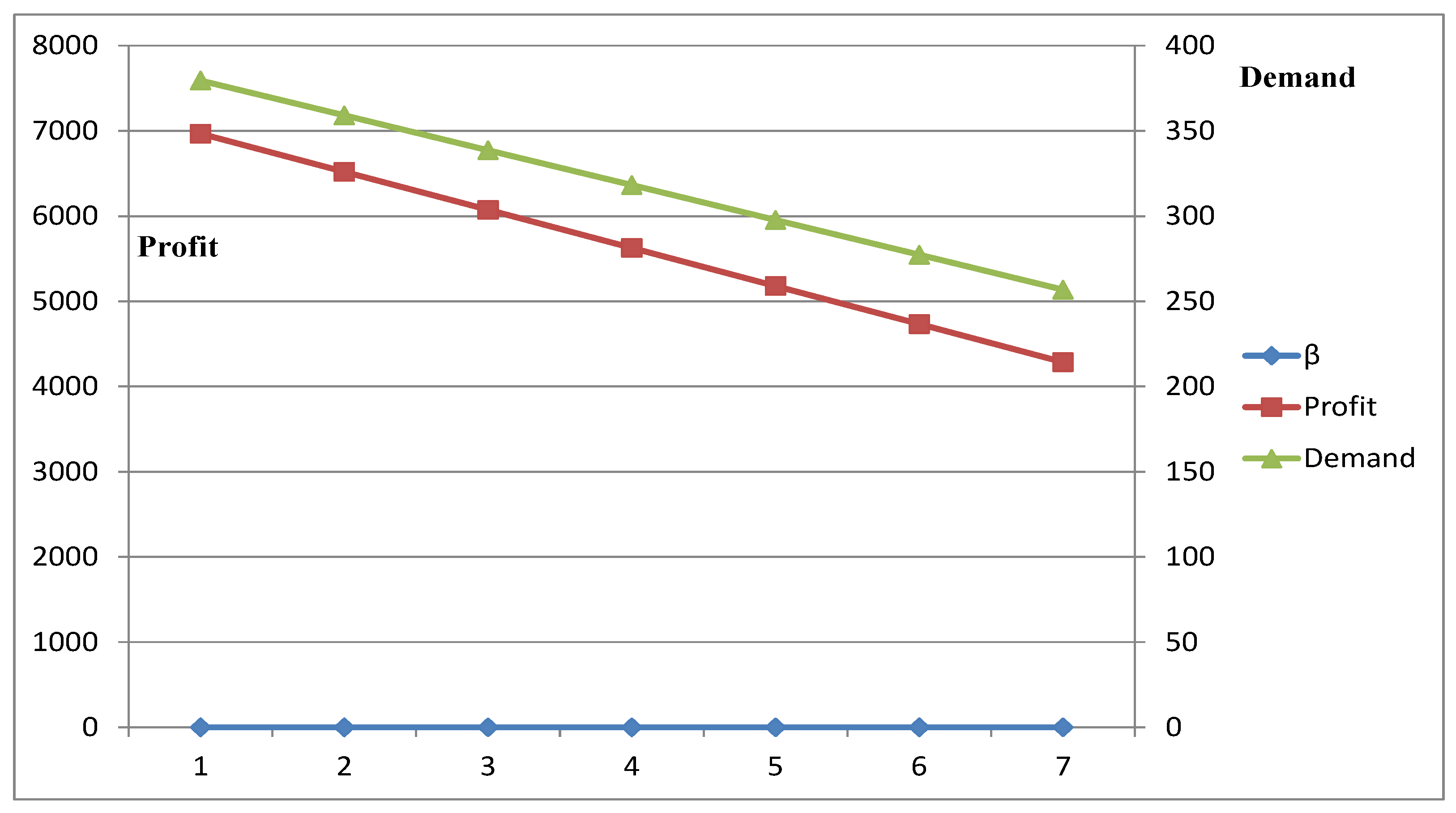
Taking = 0.1, 0.2, …, 0.7, and keeping , and as same, the sensitivity analyses for the Model-1 are presented in Table 13.
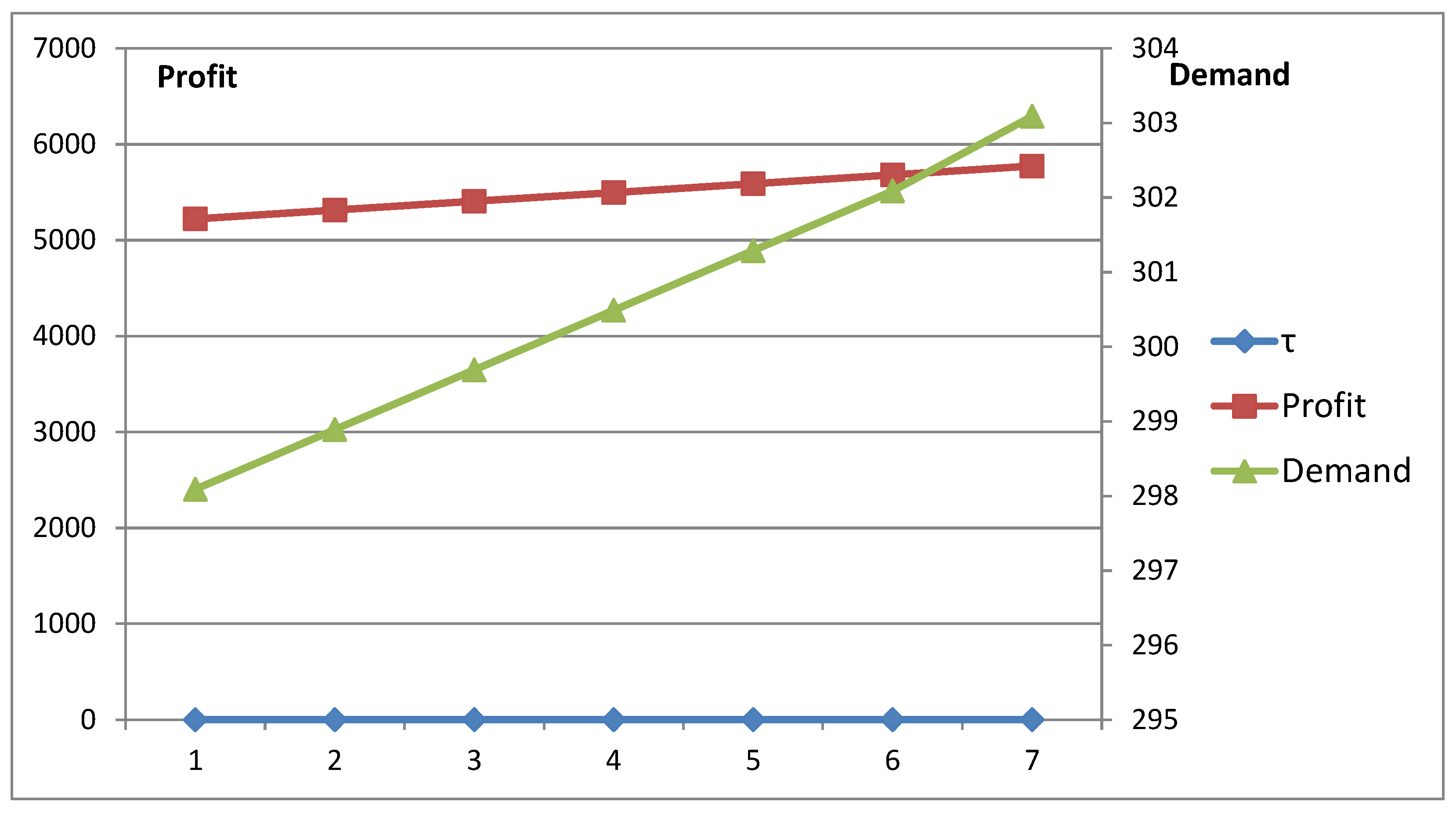
If price of items are sensitives with = 0.1, 0.2, …, 0.7, and = 0.5, keeping and as unchanged, the sensitivity analyses for the Model-1 are presented in Table 14.
7. Discussion
Table 6, Table 7, Table 8, Table 9 and Table 10 represent the optimal solutions for given assumed values, which are self explained. From the above observation of TP-1 and TP-2, we can conclude that it yields satisfactory results and that of TP-3 and TP-4 yield almost satisfactory results. From the above observation of Table 7, we can easily infer that, with the increasing value of , the profit increases. The profit is varied for the substitute and complementary nature of the items observed from Table 11. When items are independent, then profit is maximum that is $7388.841. When item-1 and item-2 are substituted in nature with each other and item-3 is complementary nature then profit is $6966.775. However, when the item-1 and item-2 are the substitutes in nature to each other, then profit is minimum that is $5499.527.
Table 11 shows the optimal profit of model-1 for the nature of the items. This table helps the manager to make the decisions of the type of items he/she should use for his/her business policy. For the current consideration, it is observed that the existence of the complementary item is more profitable than the existence of the substitute item.
From Table 12, it is seen that the demand parameter , , and have an effect on the amount of demand. As the parameter is the negative indicator of the demand expression, its increase in value causes decreasing demand and optimum profit.
Similarly, Table 13 gives reverse calculation as is a positive (+ve) parameter present in the demand expression. The Figure 3 and Figure 4 have also established the same conclusion in Table 12 and Table 13. It is to be noticed that the coefficients of selling prices and amounts of gains do not depend on the actual amounts of these factors. Profit depends only on the deviation of the factors.
Thus, with the constant degree of substitution and complementary, profit and demand are constant though the measures of responsiveness of both merchandise are dissimilar for all cases.
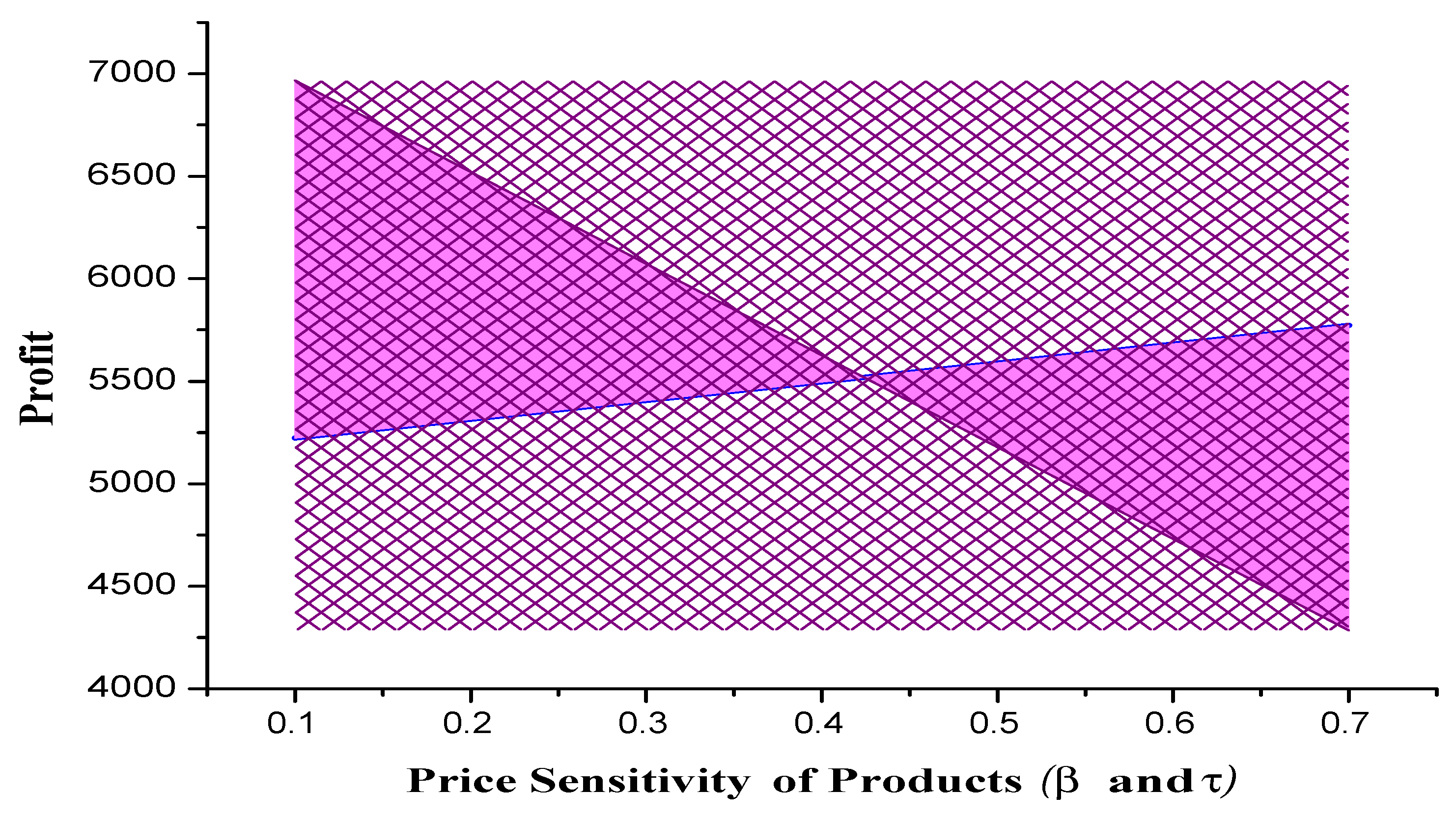
Figure 5 draws a comparison between the profit versus price of sensitivities and . It is observed that, when the price of sensitivity of product is increasing, then profit is decreasing and, when is increasing, then profit is increasing. The maximum profit is dependent on both and . Thus, it is essential to trade-off between these sensitivities parameters to achieve maximum profit when substitute and complimentary items are transported.
7.1. Discussion for Particular Models
From Table 8, when we consider only the first route of Model-II, the profit range of a corresponding 3D TP is and, from Table 9, when we take only the first conveyance of Model-II, the profit range of corresponding 3D TP is . Again when we consider only the first route and first conveyance in the Model-II, the profit range of corresponding 2D TP is .
7.2. Results of Bera et al.’s Model
8. A Real-Life Problem
M/S. Sargar studio has two shops (studios) at Midnapore Sadar, Paschim Midnapur and Digha, Purba Medinipur, India. The owner of the studio brings the photographic materials-two types of plastics and one type wooden frame material (by weight) from Kolkata, West Bengal, and Bhubaneswar, Orissa, India. There are two conveyances—bus and lorries—between sources and destinations. Two different routes for transportation are also available. Here, plastic sheets (one high quality and other one little low) are substitutes and the wooden frame is complementary. The relevant data and the results are given in Table 15. The company has sufficient storing spaces at destinations along with the sufficient budget. Here, we take the crisp values for the parameters given by the studio company (Table 16).
Out put results are without constraints are x11111 = 67.07, x11122 = 51.75, x21121 = 66.15, x21122 = 57.1, x22211 = 16.54, x22212 = 49.9, x22213 = 16.9, x11213 = 7.9, x11123 = 15.91 others are zero. Max z = 6947.52.
9. Conclusions
Renowned scientific discoveries and Research always had a practical application in the real world. Standing in the 21st century where machines, technology and industries govern the civilization, the need for sophisticated and easy techniques in the industry for optimizing products and profit is of immense importance. To further proceed and bring new ideas, we investigate a four-dimensional multifarious item transportation issue with rough interval coefficient, which maximizes the profit considering substitute and complementary products. The concept of rough interval and its properties are discussed briefly. In recent times, the rough interval has played an important role in different techniques handling vagueness for decision-making problems. The models we have discussed comprises of all earlier factors that are all considered as rough intervals. While solving the proposed model, at first, we discuss a solving procedure of a general linear programming problem with rough intervals and then we solve our model according to the concept of the above model. The rough problem is disintegrated into four classical transportation cases. We derive some special cases like a three-dimensional model and two-dimensional model to realize the problem more practically. Few examples are illustrated using LINGO 14.0 software showcasing the smooth working of the technique. We have considered a single profit maximization problem which can be extended to become a multi-objective optimization problem if we simultaneously maximize profit and minimize time. Moreover, the travelling salesman problem (TSP), Inventory routing problem, Travelling purchase problem, etc. are NP hard problems and are represented as LPPs and formulated as both single and multi-objective problems (cf. Khanra et al. [34], Manbera [35], etc.). In these problems, the travelling cost, stay charge, etc. can be taken as rough intervals and Hamzehee et al. [36] can be applied to convert to crisp models, which can be solved by heuristic methods, Genetic-Algorithms, Ant Colony Optimization, etc.
The drawback of the present methodology is that it provides a wide-range of possible profit values. The average of these possible values may give an approximate single value.
Author Contributions
S.H.J., B.D. and M.M. determined this problem and proposed the method for solutions. B.J. and G.P. did computer programming and mathematical calculations. B.J., S.H.J. and B.D. wrote the paper. M.M. and S.H.J. thoroughly checked the paper and gave interpretation to the results.
Funding
This research received no external funding.
Conflicts of Interest
The authors declare no conflict of interest.
Appendix A
In this section, some definitions and properties on Rough Intervals (RI) are given. For more details, see Hamzehee et al. [36]. An RI can be treated as a qualitative amount from a vague concept specified on a variable x in R [37], which is abstracted in the following definition.
Appendix A.1. Rough Intervals and Its Algebra
The algebraic operations applied on Rough Intervals (RIs) are taken from Moore’s Interval Arithmetic [14]. Rebolledo [13] discussed the rough interval arithmetic very significantly.
Let Q = and T = represents the rough intervals. Then, the different operations on these are:
Addition: =
Subtraction: =
Negation: −Q = , ], [,
Appendix A.2. Expected Value of a Rough Interval (Shu and Edmund [38])
Let an event X be uttered by whereas is a mathematical function in universe U in , and X is estimated by consorting to the similar relation in . The corresponding lower expected measure of X is given by
and the corresponding upper expected measure of X is given by
and the corresponding expected value of X is given by
Proposition (Shu and Edmund [38])
For any predetermined parameter , chosen by the decision maker’s (DM’s) preference, = .
Appendix A.3. General Linear Programming Problem in Rough Interval Environments
A Linear Programming Problem (LPP) in which the coefficients of the objective function and the constraints are rough intervals:
where , , , and are rough intervals. Let be the vector form of decision variables.
Now, according to Hamzehee et al. [36], here we state two theorems which help us to find the rough optimal range of the problem (1).
Let us consider two LPIC problems which are as follows.
Appendix A.3.1. LPIC-1
Appendix A.3.2. LPIC-2
The best optimal solution of the problem (1) according to Hamzehee et al. [36] and Chinneck and Ramadan [39] is i.e., LPIC-1 is found by solving:
LP1:
The best optimal solution of the problem (1) i.e., LPIC-1 is found by solving:
LP2:
The best optimal solution of the problem (1) i.e., LPIC-2 is found by solving:
LP3:
The best optimal solution of the problem (1) i.e., LPIC-2 is found by solving:
LP4:
Appendix A.3.3. Types of Solutions
There are three possible types of solutions of the problem LPIC-1 and LPIC-2 which are listed below:
- If LP-1 and LP-2 (LP-3 and LP-4) have optimal solutions, then the problem LPIC-1 (LPIC-2) has a finite bounded surely optimal (possibly optimal) range. If the maximizing value of LP-1 and LP-2 (LP-3 and LP-4) are respectively then the surely optimal range (possibly optimal range) of LPIC-1 (LPIC-2) is
- If LP-2 (LP-4) is unbounded, then LPIC-1 (LPIC-2) is unbounded.
- If LP-1 (LP-3) is infeasible, then LPIC-1 (LPIC-2) is infeasible.
Appendix A.4. Algorithm for Conversion from a Rough LPP to a Crisp LPP
The steps for converting a Rough LPP to a Crisp LPP are
Step 1: Decompose the problem (1) into two linear programming part where interval coefficients are considered i.e., LPIC-1 and LPIC-2 which are given by (2) and (3), respectively.
Step 2: In this step, LPIC-1 again transformed into two linear programming problem where crisp coefficients are considered i.e., LP-1 and LP-2 given by respectively the problems (5) and (6) and similarly from LPIC-2 as LP-3 and LP-4 given by (7) and (8), respectively.
Step 3: In this step, LP-1, LP-2, LP-3 and LP-4 to find , , and respectively. and are the solutions of LPIC-1 and LPIC-2 respectively, which are called surely optimal range and possibly optimal range.
Step 4: Here three possible consequences are given below:
- If LPIC-1 and LPIC-2 have an optimal range, then the LPRIC problem (1) has an optimal range which is a rough interval, compared to the surely optimal range
- If LPIC-1 has boundless range, then the LPRIC problem (1) has boundless range.
- If LPIC-2 is infeasible, then the LPRIC problem (1) has an infeasible solution space.
Appendix A.5. Convergence of the GRG Method
Let us consider the general nonlinear programming problem
where and are continuously differentiable functions. Any nonlinear programming theory is based on the LAGRANGE function of (19), i.e., on
where , and . Using this LAGRANGE function, the necessary optimality or Kuhn–Tucker conditions are stated in the form
which are to be approximated by the GRG algorithm. Note that the first condition can be used to eliminate , since we get . A further function which will play an important role for proving a global convergence theorem is the augmented LAGRANGE function
where , and .
Assume that the GRG Algorithm produces a sequence of iterates .
First, we note again that the boundedness of implies the boundedness of , and .
Again, we denote this set of iteration indices by . Since only finitely many different index sets and are allowed, there is an infinite subset of and index sets R, F with , , for all . For the same reason, we find a constant index set , i.e., we can also assume that and for all .
Thus, there are accumulation points and of , respectively, so that
Then, for an infinite subset
We conclude that
In addition, we have , , and
, define a Kuhn–Tucker point for problem (19).
References
- Hitchcok, F.L. The distribution of a product form several sources to numerous localities. J. Math. Phys. 1941, 20, 224–230. [Google Scholar] [CrossRef]
- Schell, E.D. Distribution of a product by several properties. In Proceedings of the 2nd Symposium in Linear Programming, DCS/Comptroller, HQ US Air Force, Washington, DC, USA, 24–25 October 1955; pp. 615–642. [Google Scholar]
- Yang, L.; Liu, P.; Li, S.; Gao, Y.; Ralescu, D.A. Reduction methods of type-2 uncertain variables and their applications to solid transportation problem. Inf. Sci. 2015, 291, 204–237. [Google Scholar] [CrossRef]
- Kocken, H.G.; Sivri, M. A simple parametric method to generate all optimal solutions of fuzzy solid transportation problem. Appl. Math. Model. 2016, 40, 4612–4624. [Google Scholar] [CrossRef]
- Halder, S.; Das, B.; Panigrahi, G.; Maiti, M. Some special fixed charge solid transportation problems of substitute and breakable items in crisp and fuzzy environments. Comput. Ind. Eng. 2017, 111, 272–281. [Google Scholar] [CrossRef]
- Das, A.; Bera, U.K.; Maiti, M. A Profit Maximizing Solid Transportation Model Under a Rough Interval Approach. IEEE Trans. Fuzzy Syst. 2017, 25, 485–498. [Google Scholar] [CrossRef]
- Bera, S.; Giri, P.K.; Jana, D.K.; Basu, K.; Maiti, M. Multi-item 4D-TPs under budget constraint using rough interval. Appl. Soft Comput. 2018, 71, 364–385. [Google Scholar] [CrossRef]
- Sarkar, M.; Lee, Y.H. Optimum pricing strategy for complementary products with reservation price in a supply chain model. J. Ind. Manag. Optim. 2017, 13, 1553–1586. [Google Scholar] [CrossRef]
- Sarkar, M.; Hur, S.; Sarkar, B. Effects of Variable Production Rate and Time-Dependent Holding Cost for Complementary Products in Supply Chain Model. Math. Probl. Eng. 2017, 2017, 2825103. [Google Scholar] [CrossRef]
- Khanna, A.; Kishore, A.; Sarkar, B.; Jaggi, C. Supply Chain with Customer-Based Two-Level Credit Policies under an Imperfect Quality Environment. Mathematics 2018, 6, 299. [Google Scholar] [CrossRef]
- Hirsch, W.M.; Dantzig, G.B. The fixed charge problem. Naval Res. Logist. NRL 1968, 15, 413–424. [Google Scholar] [CrossRef]
- Kowalski, K.; Lev, B. On step fixed-charge transportation problem. Omega 2008, 36, 913–917. [Google Scholar] [CrossRef]
- Gen, M.; Li, Y.Z. Spanning tree-based genetic algorithm for bicriteria transportation problem. Comput. Ind. Eng. 1998, 35, 531–534. [Google Scholar] [CrossRef]
- Verma, R.; Biswal, M.P.; Biswas, A. Fuzzy programming technique to solve multi-objective transportation problems with some non-linear membership functions. Fuzzy Sets Syst. 1997, 91, 37–43. [Google Scholar] [CrossRef]
- Shafaat, A.; Goyal, S.K. Resolution of degeneracy in transportation problems. J. Oper. Res. Soc. 1988, 39, 411–413. [Google Scholar] [CrossRef]
- Saad, O.M.; Abbas, S.A. A parametric study on transportation problem under fuzzy environment. J. Fuzzy Math. 2003, 11, 115–124. [Google Scholar]
- Iqbal, M.W.; Sarkar, B. Recycling of lifetime dependent deteriorated products through different supply chains. RAIRO-Oper. Res. 2019, 53, 129–156. [Google Scholar] [CrossRef]
- Sarkar, B.; Mandal, B.; Sarkar, S. Preservation of deteriorating seasonal products with stock-dependent consumption rate and shortages. J. Ind. Manag. Optim. 2017, 13, 187–206. [Google Scholar] [CrossRef]
- Pramanik, S.; Maity, K.; Jana, D.K. A multi-objective solid transportation problem with reliability for damageable items in random fuzzy environment. Int. J. Oper. Res. 2018, 31, 1–23. [Google Scholar] [CrossRef]
- Sarkar, B.; Shaw, B.K.; Kim, T.; Mitali, S.; Shin, D. An integrated inventory model with variable transportation cost, two-stage inspection, and defective items. J. Ind. Manag. Optim. 2017, 13, 1975–1990. [Google Scholar] [CrossRef]
- Ojha, A.; Mondal, S.K.; Maiti, M. A solid transportation problem with partial nonlinear transportation cost. J. Appl. Comput. Math. 2014, 3, 1–6. [Google Scholar]
- Ishfaq, N.; Sayed, S.; Akram, M.; Smarandache, F. Notions of Rough Neutrosophic Digraphs. Mathematics 2018, 6, 18. [Google Scholar] [CrossRef]
- Bit, A.K.; Biswal, M.P.; Alam, S.S. Fuzzy programming approach to multiobjective solid transportation problem. Fuzzy Sets Syst. 1993, 57, 183–194. [Google Scholar] [CrossRef]
- Jiménez, F.; Verdegay, J.L. Solving fuzzy solid transportation problems by an evolutionary algorithm based parametric approach. Eur. J. Oper. Res. 1999, 117, 485–510. [Google Scholar] [CrossRef]
- Li, T.H.S.; Su, Y.T.; Lai, S.W.; Hu, J.J. Walking motion generation, synthesis, and control for biped robot by using PGRL, LPI, and fuzzy logic. IEEE Trans. Syst. Man Cybern. Part B Cybern. 2011, 41, 736–748. [Google Scholar] [CrossRef]
- Dey, A.; Pal, A.; Pal, T. Interval type 2 fuzzy set in fuzzy shortest path problem. Mathematics 2016, 4, 62. [Google Scholar] [CrossRef]
- Kundu, P.; Kar, S.; Maiti, M. Fixed charge transportation problem with type-2 fuzzy variables. Inf. Sci. 2014, 255, 170–186. [Google Scholar] [CrossRef]
- Tao, Z.; Xu, J. A class of rough multiple objective programming and its application to solid transportation problem. Inf. Sci. 2012, 188, 215–235. [Google Scholar] [CrossRef]
- Haley, K.B. New methods in mathematical programming—The solid transportation problem. Oper. Res. 1962, 10, 448–463. [Google Scholar] [CrossRef]
- Ojha, A.; Das, B.; Mondal, S.K.; Maiti, M. A multi-item transportation problem with fuzzy tolerance. Appl. Soft Comput. 2013, 13, 3703–3712. [Google Scholar] [CrossRef]
- Liu, P.; Yang, L.; Wang, L.; Li, S. A solid transportation problem with type-2 fuzzy variables. Appl. Soft Comput. 2014, 24, 543–558. [Google Scholar] [CrossRef]
- Giri, P.K.; Maiti, M.K.; Maiti, M. Fully fuzzy fixed charge multi-item solid transportation problem. Appl. Soft Comput. 2015, 27, 77–91. [Google Scholar] [CrossRef]
- Schittkiowski, K. On the convergence of a generalized reduced gradient algorithm for nonlinear programming problems. Optimization 1986, 17, 731–755. [Google Scholar] [CrossRef]
- Khanra, A.; Maiti, M.K.; Maiti, M. Profit maximization of TSP through a hybrid algorithm. Comput. Ind. Eng. 2015, 88, 229–236. [Google Scholar] [CrossRef]
- Manerba, D.; Mansini, R.; Riera-Ledesma, J. The traveling purchaser problem and its variants. Eur. J. Oper. Res. 2017, 259, 1–18. [Google Scholar] [CrossRef]
- Hamzehee, A.; Yaghoobi, M.A.; Mashinchi, M. Linear programming with rough interval coefficients. J. Intell. Fuzzy Syst. 2014, 26, 1179–1189. [Google Scholar]
- Rebolledo, M. Rough intervals—Enhancing intervals for qualitative modeling of technical systems. Artif. Intell. 2006, 170, 667–685. [Google Scholar] [CrossRef]
- Xiao, S.; Lai, E.M.K. A rough programming approach to power-balanced instruction scheduling for VLIW digital signal processors. IEEE Trans. Signal Process. 2008, 56, 1698–1709. [Google Scholar] [CrossRef]
- Chinneck, J.W.; Ramadan, K. Linear programming with interval coefficients. J. Oper. Res. Soc. 2000, 51, 209–220. [Google Scholar] [CrossRef]
Figure 1.
Pictorial representation of a four-dimensional transportation model.

Figure 2.
Optimization flowchart of 4D-TP under rough interval coefficients.

Figure 3.
Profit vs. demand with respect to .

Figure 4.
Profit vs. demand with respect to .

Figure 5.
Profit vs. demand with respect to and .


Table 1.
Year wise investigations of TP and STP.
| References’ | Different Kind of TP | Item | Fixed Charge | Space Constraint | Budget Constraint | Different Kind of Environment |
|---|---|---|---|---|---|---|
| Hitchcock et al. [1] | 2-dimension | one | × | × | - | crisp |
| Schell [2] | 3-dimension | one | × | × | - | crisp |
| Haley [29] | 3-dimension | one | × | × | - | crisp |
| Hirsch and Dantzig [11] | 2-dimension | one | ✓ | × | × | crisp |
| Verma et al. [14] | 2-dimension | one | × | × | × | fuzzy |
| Shafaat and Goyal [15] | 2-dimension | one | × | × | × | crisp |
| Saad and Abbas [16] | 2-dimension | one | × | × | × | fuzzy |
| Jimenez et al. [24] | 3-dimension | one | × | × | × | fuzzy |
| Tao et al. [28] | 3-dimension | one | × | × | × | rough |
| Ojha et al. [30] | 2-dimension | multi-item | × | × | ✓ | fuzzy |
| Liu et al. [31] | 3-dimension | one | × | × | × | type-2 fuzzy |
| Kundu et al. [27] | 3-dimension | multi-item | × | × | × | type-2 fuzzy |
| Yang et al. [3] | 2-dimension | one | ✓ | × | × | fuzzy |
| Giri et al. [32] | 3-dimension | multi-item | ✓ | × | × | fuzzy |
| Kocken et al. [4] | 3-dimension | one | × | × | × | fuzzy |
| Das et al. [6] | 3-dimension | one | × | × | × | rough |
| Present Paper | 4-dimensional | multi-item | ✓ | ✓ | ✓ | rough |
Table 2.
Unit cost of transportation , fixed charges , breakability for proposed Models.
| p | 1 | 2 | |||||||
|---|---|---|---|---|---|---|---|---|---|
| k | 1 | 2 | 1 | 2 | |||||
| i/j | 1 | 2 | 1 | 2 | 1 | 2 | 1 | 2 | |
| Model-I | |||||||||
| (Crisp Model) | |||||||||
| 1 | 0.5 | 2.1 | 1.7 | 1.12 | 0.85 | 0.5 | 1.38 | 1.28 | |
| 2 | 1.21 | 1.28 | 2.05 | 0.6 | 1.65 | 2.72 | 1.66 | 1.78 | |
| 1 | 1.5 | 2.25 | 2.0 | 1.3 | 0.08 | 0.7 | 1.05 | 1.25 | |
| 2 | 1.05 | 2.15 | 2.2 | 0.9 | 1.35 | 2.25 | 1.85 | 0.98 | |
| 1 | 1.3 | 1.2 | 1.91 | 1.2 | 0.9 | 0.94 | 0.73 | 0.93 | |
| 2 | 1.22 | 1.3 | 2 | 0.7 | 1.8 | 3 | 1.8 | 1.8 | |
| 1 | 0.01 | 0.01 | 0.01 | 0.01 | 0.02 | 0.02 | 0.02 | 0.02 | |
| 2 | 0.01 | 0.01 | 0.01 | 0.01 | 0.02 | 0.02 | 0.02 | 0.02 | |
| 1 | 0.01 | 0.01 | 0.01 | 0.01 | 0.02 | 0.02 | 0.02 | 0.02 | |
| 2 | 0.01 | 0.01 | 0.01 | 0.01 | 0.02 | 0.02 | 0.02 | 0.02 | |
| 1 | 0.01 | 0.01 | 0.01 | 0.01 | 0.02 | 0.02 | 0.02 | 0.02 | |
| 2 | 0.01 | 0.01 | 0.01 | 0.01 | 0.02 | 0.02 | 0.02 | 0.02 | |
| 1 | 1.9 | 1.7 | 1.1 | 1.3 | 1.2 | 1.4 | 0.3 | 1.8 | |
| 2 | 1.2 | 1.85 | 0.9 | 1.5 | 1.5 | 2.1 | 2.1 | 1.6 | |
| Model-II | |||||||||
| (Rough Model) | |||||||||
| 1 | ([1, 2], | ([0.5, 1.5], | ([1.1, 2.3], | ([0.8, 1.3], | ([1.4, 2.3], | ([0.7, 1], | ([1.2, 2], | ([1.2, 2.4], | |
| [0.7, 2.3]) | [0.5, 2]) | [1, 2.5]) | [0.5, 2]) | [1.2, 2.8] ) | [0.5, 1.5]) | [1.2, 2.3]) | [1, 3]) | ||
| 2 | ([1.2, 2.5], | ([0.9, 2], | ([1.1, 2], | ([1, 2], | ([1.1, 2.2], | ([1, 2.5], | ([0.9, 2.1], | ([1.3, 2.5], | |
| [1, 3]) | [0.5, 3.2]) | [0.7, 2.5]) | [0.9, 2.6]) | [1, 2.7]) | [0.3, 3]) | [0.7, 2.8]) | [1.1, 3.5]) | ||
| 1 | ([1.3, 2.7], | ([1.7, 2.8], | ([1.5, 2.5], | ([1.6, 2.4], | ([1.3, 3], | ([1.4, 2], | ([1.5, 2.6], | ([1.8, 2.7], | |
| [1, 3]) | [1.2, 3.1]) | [1.4, 3.1]) | [1.5, 3.5]) | [1.2, 3.5]) | [1.1, 2.5]) | [1.3, 3]) | [1.6, 3.4] | ||
| 2 | ([1.5, 2.5], | ([1.3, 3], | ([1.7, 2.7], | ([1.4, 3], | ([2, 2.7], | ([1.3, 2.2], | ([1.6, 2.1], | ([1.6, 2.5], | |
| [1, 3.5]) | [1.1, 3.7]) | [1.5, 3]) | [1.2, 3.2]) | [1.8, 3]) | [1, 2.5]) | [1.5, 2.8]) | [1.4, 2.8]) | ||
| 1 | ([0.5, 1.5], | ([0.7, 1], | ([0.7, 1.3], | ([0.8, 1.6], | ([0.7, 1.4], | ([0.8, 1.8], | ([1, 1.5], | ([0.9, 1.8], | |
| [0.5, 2]) | [0.6, 1.5]) | [0.4, 2]) | [0.3, 1.7]) | [0.6, 2]) | [0.3, 2.3]) | [0.8, 1.8]) | [0.7, 2.1]) | ||
| 2 | ([0.2, 0.5], | ([0.3, 0.6], | ([0.9, 1.7], | ([1, 1.5], | ([0.9, 1.5], | ([0.5, 1.6], | ([0.4, 0.9], | ([1, 1.7], | |
| [0.1, 1]) | [0.2, 1]) | [0.6, 1.8]) | [0.5, 1.6]) | [0.4, 1.9]) | [0.2, 2]) | [0.2, 1]) | [0.5, 2]) | ||
Table 3.
Parametric values for the Models.
| Models | Source | Demand | Capacities. of Conveyance. |
|---|---|---|---|
| -I | (90, 80, 85 | (75, 73, 70, | (90, 85, 80 |
| 85, 75, 70) | 65, 63, 60) | 85, 70, 75) | |
| {([89.5, 90], [88.6, 91]), | {([74, 75], [73.6, 76]), | {([89, 90], [88, 91]), | |
| ([79.6, 80], [78.5, 81.3]), | ([72.6, 73], [72, 74]), | ([84, 85], [83, 86.3]), | |
| ([84.7, 85], [83.5, 86]), | ([69.4, 70], [68.7, 71]), | ([79, 80], [78, 81.3]), | |
| -II | ([84.4, 85], [83.6, 86]), | ([64.5,65], [64, 66]), | ([84, 85], [83, 86.3]), |
| ([74, 75], [73.6, 76]), | ([62.4, 63], [62, 64]), | ([69, 70], [68, 71]), | |
| ([69.4, 70], [68.7, 71])} | ([59.4, 60], [59, 61])} | ([74, 75], [73, 76])} |
Table 4.
Parametric values for the Models.
| Models | Purchasing Costs | Unit Selling Price | Budget | |
|---|---|---|---|---|
| -I | (9, 8, 10 | (52, 30, 24, | (3000, 2500, 2700) | (510, 520, 525) |
| 6, 7, 8.5) | 46, 28, 20) | |||
| {([8.3, 9], [8, 10]), | {([51.5, 52], [51, 53]), | {([8250,5000], | {([509.6,510.3], | |
| ([7.5, 8], [7, 9]), | ([29, 30], [28, 31]), | [7500,8600]), | [509, 511]), | |
| ([9, 10], [8, 10.5]), | ([23.5, 24], [23, 25]), | ([7500,8600], | ([519.4,520], | |
| -III | ([5.5, 6], [5, 7]), | ([45.5,45], [45.3, 46]), | [4500,4600]), | [519, 521]), |
| ([6.5, 7], [6, 7.8]), | ([27.4, 28], [27, 29]), | ([4400,4700]), | ([524, 525]), | |
| ([8, 8.5], [7.5, 9])} | ([19.5, 20], [19.1, 21])} | [4400,4700])} | [523,526])} |
Table 5.
Distances () of the routes for the Models.
| Route | Destination | Origin-1 | Origin-2 |
|---|---|---|---|
| 1 | 1 | 35 | 30 |
| 2 | 40 | 25 | |
| 2 | 1 | 30 | 35 |
| 2 | 25 | 30 |
Table 6.
Optimum results for Model-I and Model-II (Hamzehee Method) by Lingo.
| Models | Crisp Model | 4D Rough Model | |||
|---|---|---|---|---|---|
| TP-1 | TP-2 | TP-3 | TP-4 | ||
| Optimal profit | 6966.775 | 5293.95 | 8058.61 | 4109.11 | 9130.81 |
| Set-1 | Set-2 | Set-3 | Set-4 | ||
| x11111 = 63.07 | x11221 = 14.04 | x11122 = 48.7 | x11111 = 54.4 | x11111 = 52.44 | |
| x11122 = 52.75 | x12112 = 46 | x11221 = 65.3 | x11221 = 32.2 | x11112 = 25.41 | |
| x11222 = 8.75 | x12211 = 29.96 | x11222 = 49.6 | x11222 = 17.9 | x11222 = 19.9 | |
| x21121 = 67.15 | x21121 = 50.46 | x12211 = 22.1 | x12211 = 0.2 | x12112 = 9.09 | |
| x21122 = 47.1 | x21122 = 21.84 | x12221 = 42.2 | x21121 = 20.3 | x12211 = 62.24 | |
| x22211 = 27.74 | x21211 = 33.04 | x21111 = 44 | x21122 = 19.9 | x21121 = 54.71 | |
| x22212 = 39.9 | x21222 = 45.16 | x21121 = 9.80 | x22211 = 31.31 | x21122 = 65.91 | |
| x22213 = 26.9 | x21223 = 26.07 | x21123 = 14.80 | x22213 = 2.23 | x21123 = 27.09 | |
| x11213 = 7.9 | x21123 = 27.16 | x22123 = 23.80 | x22113 = 62.04 | x22123 = 15.09 | |
| x11123 = 15.91 | x11123 = 15.91 | x11123 = 15.91 | x22212 = 18.65 | x21113 = 28.51 | |
| others are zero | others are zero | x21122 = 33.4 | other are zero | x21211 = 8.29 | |
| x22212 = 14.9 | x22212 = 31.21 | ||||
| other are zero | other are zero |
Table 7.
Optimum results for Model-II (Expected Value Technique) by Lingo.
| = 0.0 | = 0.2 | = 0.4 | = 0.5 | = 0.6 | = 0.8 | = 1.0 |
|---|---|---|---|---|---|---|
| 6351.76 | 6393.95 | 6412.61 | 6463.11 | 6488.81 | 6504.54 | 6523.54 |
| x11111 = 32.75 | x11111 = 32.84 | x11111 = 32.86 | x11111 = 28.85 | x11111 = 28.14 | x11111 = 28.09 | x11111 = 28.92 |
| x11222 = 30.33 | x11222 = 30.33 | x22212 = 27.46 | x11222 = 30.13 | x11222 = 30.02 | x11222 = 30.33 | x11222 = 30.33 |
| x12211 = 45.65 | x12211 = 45.576 | x12211 = 45.52 | x12211 = 45.5 | x12211 = 45.48 | x12211 = 45.44 | x12211 = 45.40 |
| x21121 = 52.20 | x21121 = 52.16 | x21121 = 52.13 | x21111 = 39.2 | x21113 = 39.09 | x21113 = 42.76 | x21113 = 42.76 |
| x21122 = 10.8 | x21122 = 18.75 | x21122 = 10.712 | x21121 = 32.3 | x21121 = 32.24 | x21121 = 54.05 | x21121 = 54.21 |
| x21223 = 30.74 | x21223 = 30.44 | x21223 = 30.04 | x21123 = 14.9 | x21123 = 14.71 | x21123 = 24.01 | x21123 = 24.32 |
| x22111 = 23.9 | x22111 = 23.13 | x22111 = 23.80 | x21222 = 23.14 | x21222 = 23.37 | x21222 = 23.41 | x21222 = 33.51 |
| x22213 = 32.9 | x22213 = 32.06 | x22213 = 32.16 | x22213 = 32.16 | x22213 = 32.22 | x22113 = 32.8 | x22113 = 41.05 |
| and all | and all | x22212 = 18.9 | x22212 = 27.46 | x21211 = 27.49 | and all | and all |
| others | others | and all others | and all | x22212 = 5.61 | others are zero | others are zero |
| variables | variables | variables | others | and all | ||
| are zero | are zero | are zero | variables | others are zero | ||
| are zero |
Table 8.
Optimum results for existence of different constraints (Expected Value Technique) by Lingo.
Table 8.
Optimum results for existence of different constraints (Expected Value Technique) by Lingo.
| Results without Space and Budget | Results with Space and without Budget | Results without Space and with Budget |
|---|---|---|
| x11111 = 42.75 | x11221 = 22.84 | x11211 = 19.06 |
| x11212 = 13.33 | x11222 = 32.04 | x21222 = 53.33 |
| x12211 = 25.65 | x12211 = 45.57 | x22212 = 14.9 |
| x21121 = 52.20 | x21121 = 52.16 | x21121 = 32.13 |
| x21122 = 10.8 | x21122 = 10.75 | x21122 = 10.71 |
| x21223 = 57.74 | x21223 = 30.44 | x21213 = 24.54 |
| x22112 = 43.9 | x22112 = 53.16 | x22112 = 53.80 |
| x22213 = 32.9 | x22213 = 32.16 | x22213 = 32.16 |
| x12213 = 12.9 | x12213 = 12.9 | x21122 = 27.4 |
| x11123 = 21.17 | x11123 = 11.17 | x11123 = 31.12 |
| and all others | and all others | and all others |
| variables are zero | variables are zero | variables are zero |
| Optimal profit 6579.135 | Optimal profit 6529.07 | Optimal profit 6513.513 |
Table 9.
Optimum results of the STP Model ignoring route.
| 823.76 | 1263.95 | 323.61 | 2623.21 |
|---|---|---|---|
| x1111 = 14.22 | x1111 = 0.82 | x1111 = 16.52 | x1111 = 18.04 |
| x1112 = 0.75 | x1112 = 4.19 | x1112 = 4.43 | x1112 = 9.12 |
| x1121 = 0.05 | x1121 = 6.26 | x1121 = 0.72 | x1121 = 0.21 |
| x1122 = 11.225 | x1122 = 12.06 | x1122 = 0.92 | x1122 = 11.42 |
| x1211 = 8.25 | x1211 = 0.36 | x1211 = 0.26 | x1211 = 0.53 |
| x1212 = 0.65 | x1212 = 0.16 | x1212 = 0.36 | x1212 = 0.43 |
| x1222 = 0.25 | x1222 = 5.06 | x1222 = 0.16 | x1221 = 8.12 |
| x2111 = 0.51 | x2111 = 0.06 | x2111 = 0.91 | x1222 = 0.09 |
| x2112 = 0.62 | x2112 = 8.03 | x2112 = 0.82 | x2111 = 5.05 |
| x2121 = 29.74 | x2121 = 0.4 | x2121 = 4.24 | x2112 = 27.3 |
| x2122 = 5.9 | x2122 = 0.44 | x2122 = 0.80 | x2121 = 8.44 |
| x2211 = 0.65 | x2211 = 5.26 | x2211 = 0.6 | x2122 = 5.32 |
| x2213 = 10.25 | x2213 = 0.96 | x2213 = 0.03 | x2213 = 14.76 |
| x2221 = 0.35 | x2221 = 4.81 | x2221 = 6.6 | x2212 = 5.75 |
| x2223 = 5.05 | x2223 = 5.76 | x2223 = 7.6 | x2223 = 9.2 |
| others zero | others zero | others zero | others zero |
Table 10.
Optimum results of the STP Model ignoring conveyance.
| 623.76 | 1103.95 | 383.61 | 2056.32 |
|---|---|---|---|
| x1111 = 0.24 | x1111 = 0.84 | x1111 = 0.57 | x1111 = 14.17 |
| x1112 = 0.76 | x1112 = 0.11 | x1112 = 0.33 | x111 = 0.42 |
| x1121 = 0.05 | x1121 = 0.26 | x1121 = 0.62 | x1121 = 0.43 |
| x1122 = 0.24 | x1122 = 0.26 | x1122 = 0.92 | x1122 = 0.97 |
| x1211 = 0.23 | x1211 = 0.46 | x1211 = 0.36 | x1211 = 0.64 |
| x1212 = 0.54 | x1212 = 0.16 | x1212 = 0.46 | x1212 = 0.54 |
| x1222 = 0.25 | x1222 = 14.06 | x1222 = 0.26 | x1223 = 0.17 |
| x2111 = 0.51 | x2111 = 0.06 | x2111 = 0.91 | x1333 = 0.65 |
| x2112 = 0.62 | x2112 = 42.03 | x2112 = 0.82 | x1213 = 0.42 |
| x2121 = 32.74 | x2121 = 0.4 | x2121 = 44.24 | x2121 = 41.53 |
| x2122 = 20.9 | x2122 = 0.44 | x2122 = 0.80 | x2122 = 10.42 |
| x2211 = 7.65 | x2211 = 10.26 | x2211 = 0.6 | x2211 = 0.95 |
| x2213 = 0.25 | x2213 = 0.96 | x2213 = 0.03 | x221 = 0.94 |
| x2221 = 0.35 | x2221 = 25.11 | x2221 = 1.6 | x2221 = 0.79 |
| x2223 = 0.05 | x2223 = 8.76 | x2223 = 12.6 | x2222 = 0.57 |
| others zero | others zero | others zero | others zero |
Table 11.
Optimum solutions for 2D-TP Model.
| 4113.06 | 8093.95 | 453.61 | 8243.93 |
|---|---|---|---|
| x111 = 63 | x111 = 64.82 | x111 = 63.32 | x111 = 62 |
| x112 = 52 | x112 = 19.26 | x112 = 2.62 | x112 = 17.2 |
| x121 = 50.0 | x121 = 16.36 | x121 = 0.67 | x211 = 8 |
| x122 = 5.0 | x122 = 0.70 | x122 = 0.32 | x223 = 23 |
| x211 = 6 | x211 = 23.8 | x211 = 2.18 | x222 = 26.21 |
| x213 = 5.5 | x213 = 5.0 | x213 = 2.23 | other zero |
| x221 = 16.5 | x221 = 8.0 | x221 = 4.15 | |
| x223 = 19.5 | x223 = 27.4 | x223 = 4.32 | |
| other zero | other zero | other zero |
Table 12.
Results for the different combinations of substitute and complementary items.
| Problem | Independent | Substitute | Complementary | Profit for Model-1 |
|---|---|---|---|---|
| 1 | Item-1, Item-2, Item-3 | 7388.841 | ||
| 1 | Item-1, Item-2 | Item-3 | 6966.775 | |
| 2 | Item-1, Item-2 | 5497.527 | ||
| 3 | Item-1, Item-3 | 6021.859 | ||
| 4 | Item-2, Item-3 | 5952.067 |
Table 13.
Sensitivity analysis (w.r.t ).
| Set | Maximum Profit | Demand | |||
|---|---|---|---|---|---|
| 1 | 0.052 | 0.052 | 0.1 | 6966.68 | 379.542 |
| 0.052 | 0.052 | 0.2 | 6519.775 | 359.084 | |
| 0.052 | 0.052 | 0.3 | 6072.868 | 338.627 | |
| 0.052 | 0.052 | 0.4 | 5625.962 | 318.1696 | |
| 0.052 | 0.052 | 0.5 | 5179.055 | 297.712 | |
| 0.052 | 0.052 | 0.6 | 4732.149 | 277.254 | |
| 0.052 | 0.052 | 0.7 | 4285.242 | 256.79 |
Table 14.
Sensitivity Analysis (w.r.t ).
| Set | Maximum Profit | Demand | |||
|---|---|---|---|---|---|
| 1 | 0.1 | 0.052 | 0.5 | 5223.015 | 298.09 |
| 0.2 | 0.052 | 0.5 | 5314.598 | 298.89 | |
| 0.3 | 0.052 | 0.5 | 5406.181 | 299.69 | |
| 0.4 | 0.052 | 0.5 | 5497.76 | 300.49 | |
| 0.5 | 0.052 | 0.5 | 5589.34 | 301.29 | |
| 0.6 | 0.052 | 0.5 | 5680.93 | 302.09 | |
| 0.7 | 0.052 | 0.5 | 5772.513 | 303.89 |
Table 15.
Unit cost of transportation , fixed charges , breakability for proposed Models.
| p | 1 | 2 | |||||||
|---|---|---|---|---|---|---|---|---|---|
| 1 | 2 | 1 | 2 | ||||||
| 1 | 2 | 1 | 2 | 1 | 2 | 1 | 2 | ||
| Model-I | |||||||||
| (Crisp Model) | |||||||||
| 1 | 0.15 | 1.1 | 1.2 | 0.12 | 0.85 | 0.5 | 1.38 | 1.28 | |
| 2 | 0.21 | 1.3 | 2.5 | 0.6 | 1.65 | 1.72 | 0.66 | 0.78 | |
| 1 | 1.5 | 2.25 | 2.0 | 1.3 | 0.08 | 0.7 | 1.05 | 1.25 | |
| 2 | 0.25 | 0.25 | 1.2 | 1.9 | 1.35 | 1.25 | 1.85 | 0.98 | |
| 1 | 1.3 | 1.2 | 1.91 | 1.2 | 0.9 | 0.94 | 0.73 | 0.93 | |
| 2 | 0.52 | 1.53 | 1.2 | 0.7 | 1.8 | 0.53 | 1.9 | 0.98 | |
| 1 | 0.01 | 0.01 | 0.02 | 0.03 | 0.01 | 0.02 | 0.01 | 0.02 | |
| 2 | 0.02 | 0.01 | 0.03 | 0.04 | 0.02 | 0.01 | 0.03 | 0.02 | |
| 1 | 0.04 | 0.03 | 0.01 | 0.02 | 0.05 | 0.01 | 0.02 | 0.03 | |
| 2 | 0.05 | 0.04 | 0.02 | 0.03 | 0.02 | 0.01 | 0.03 | 0.02 | |
| 1 | 0.01 | 0.01 | 0.01 | 0.01 | 0.02 | 0.02 | 0.02 | 0.02 | |
| 2 | 0.04 | 0.05 | 0.02 | 0.03 | 0.01 | 0.02 | 0.04 | 0.02 | |
| 1 | 1.1 | 1.4 | 1.5 | 1.0 | 1.2 | 1.4 | 0.3 | 1.8 | |
| 2 | 1.3 | 1.5 | 0.9 | 1.1 | 1.3 | 2.1 | 2.1 | 1.02 | |
Table 16.
Parametric values for the Models.
| Models | Source | Demand | Capacities. of Conveyance. | Purchasing Costs | Unit Selling Price |
|---|---|---|---|---|---|
| -I | (85, 75, 80 | (60, 70, 75, | (86, 89, 90 | (45, 48, 51 | (132, 145, 124, |
| 83, 72, 68) | 62, 64, 59) | 81, 65, 70) | 36, 47, 58.5) | 126, 135, 137) |
© 2019 by the authors. Licensee MDPI, Basel, Switzerland. This article is an open access article distributed under the terms and conditions of the Creative Commons Attribution (CC BY) license (http://creativecommons.org/licenses/by/4.0/).
Share and Cite
MDPI and ACS Style
Halder Jana, S.; Jana, B.; Das, B.; Panigrahi, G.; Maiti, M. Constrained FC 4D MITPs for Damageable Substitutable and Complementary Items in Rough Environments. Mathematics 2019, 7, 281. https://doi.org/10.3390/math7030281
AMA Style
Halder Jana S, Jana B, Das B, Panigrahi G, Maiti M. Constrained FC 4D MITPs for Damageable Substitutable and Complementary Items in Rough Environments. Mathematics. 2019; 7(3):281. https://doi.org/10.3390/math7030281
Chicago/Turabian StyleHalder Jana, Sharmistha, Biswapati Jana, Barun Das, Goutam Panigrahi, and Manoranjan Maiti. 2019. "Constrained FC 4D MITPs for Damageable Substitutable and Complementary Items in Rough Environments" Mathematics 7, no. 3: 281. https://doi.org/10.3390/math7030281
Note that from the first issue of 2016, this journal uses article numbers instead of page numbers. See further details here.