Fractional vs. Ordinary Control Systems: What Does the Fractional Derivative Provide? ^†

Abstract

The concept of a fractional derivative is not at all intuitive, starting with not having a clear geometrical interpretation. Many different definitions have appeared, to the point that the need for order has arisen in the field. The diversity of potential applications is even more overwhelming. When modeling a problem, one must think carefully about what the introduction of fractional derivatives in the model can provide that was not already adequately covered by classical models with integer derivatives. In this work, we present some examples from control theory where we insist on the importance of the non-local character of fractional operators and their suitability for modeling non-local phenomena either in space (action at a distance) or time (memory effects). In contrast, when we encounter completely different nonlinear phenomena, the introduction of fractional derivatives does not provide better results or further insight. Of course, both phenomena can coexist and interact, as in the case of hysteresis, and then we would be dealing with fractional nonlinear models.

1. Introduction

It is quite frequent to find research works in which, after introducing an existing model based on ODEs, the derivatives are directly substituted by some fractional derivatives. The argument is that the fractional model will represent the original system more closely by choosing some particular exponents of the fractional derivatives. However, the introduction of fractional derivatives is not trivial and should be considered carefully. Firstly, in some cases, there is no clear explanation of the fractional nature of the model. Besides, if an explanation of the model’s fractional nature exists, deduction from a first-principles argument is usually missing in the exposition. Secondly, the introduction of fractional derivatives is not in itself a better strategy, and lastly, but not least, the complexity of the model increases since the fractional derivative concept is not really intuitive.

Fractional derivatives lack a clear geometric interpretation, as is the case in the traditional derivative, although some proposals exist in this sense [1,2]. Besides, there is not a single formal definition of a fractional derivative, which makes things a little more complicated for potential users. There exists a great variety of them [3,4], although there are basically three: Riemann-Liouville, Gronwald-Letnikov, and Caputo definitions. However, when modeling a problem and after we have established their use and presented some advantages, it is not immediate to know which definition will be better to choose [5,6].

Fractional derivatives are usually considered for modeling processes of mass transport, diffusion, optics, and other phenomena with memory effects; see, for instance [7,8,9,10,11]. With the inclusion of these derivatives, fractional-order models have demonstrated its advantages when modeling supercapacitator capacitances [12] and controllers for temperature [13], DC motors [14], or RC, LC, and RLC electric circuits [15]. These models have also been implemented, as it is the case of the fractional-order inductor [16,17] and have demonstrated better characteristics and greater design freedom in the case of temperature control [18], wireless power transfer systems [19], battery charges [20], or memristors [21].

In this paper, applications are considered in the framework of control engineering, both control design and modeling, for control purposes. Thus, open systems are considered whose interaction with other systems and the environment is explicitly modeled using input and output variables besides the system state. Fractional controllers have been used to control linear and nonlinear processes with or without memory effects, i.e., non-local phenomena. Most of the designed controllers are linear. In particular, much work has been done to extend to the PID controller’s fractional case, which can be considered the control engineering workhorse in the industry. Consequently, much use is made of frequency-domain techniques. The Bode diagrams that characterize the output behavior in terms of the input signal are particularly interesting to us. Initially thought for ordinary linear systems, for which only the input signal frequency has to be considered, that they can be directly extended to the linear fractional case. For the nonlinear case, as a rule, it is not possible to use these diagrams. However, for the so-called convergent systems, a partial extension is possible. As will be explained in Section 4, this partial extension presents a new feature; the amplitude of the input signal must also be considered. This difference is crucial to explaining linear fractional systems, whose Bode diagrams depend only on frequency, as in the ordinary case and can not capture nonlinear behavior/phenomena. On the other hand, they do capture non-local phenomena, action at a distance, and memory effects. In contrast, the ordinary operator is a local one and consequently can not do so. Nevertheless, fractional systems are applied, as commented above, to all sorts of applications with or without nonlocality.

Then, a natural question arises, what are the benefits of introducing fractional controllers, apart from having one more design alternative, with respect to the classical techniques? In this work, we discuss this question with the analysis of two examples: a furnace with experimental data, and finally, an academic example. We show that using fractional derivatives does not necessarily provide a better approximation. Moreover, as shown in the academic example, when implementing them through ordinary linear filters gives rise to systems of a very high order.

The paper is organized as follows: In Section 2, we recall the concept of fractional derivative and its character as a non-local operator [22], either in space (action at a distance) or time (memory effects). Later, fractional-order models are introduced in Section 3. In Section 4, an explanation of Bode diagrams is given in a tutorial fashion for linear ordinary, linear fractional, and nonlinear convergent systems, stressing their similarities and differences. As an approximation of the fractional-order operators, we consider Oustaloup’s Filter Approximation, as described in Section 5. The calculations will be performed with FOMCON toolbox. Its use is briefly described in Section 6.

It will be important to distinguish nonlocality from nonlinearity. One of the paper aims is to clarify the following relations, see

Table 1. Phenomena and model type correspondence.

Phenomena	Model
linear and local	linear ODEs
linear and nonlocal	linear FDEs
nonlinear and local	nonlinear ODEs
nonlinear and nonlocal	nonlinear FDEs

, in the context of control modeling.

Section 7 shows an example that, when only local phenomena are present, linear fractional systems make no difference with respect to ordinary ones in order to approximate a nonlinear and local (ordinary) system. In addition, since linear fractional systems are usually implemented using an approximation by high order linear ordinary systems, problems such as overparameterization may appear. Finally, in Section 8, we draw some conclusions.

2. Fractional Derivatives

The fractional derivative is a generalization of the usual derivative for the case where non-integer derivative orders are considered [23], giving rise to a special type of integro-differential operator. Historically, the first definition of a fractional derivative was the Riemann–Liouville definition. It was developed in Abel, Riemann, and Liouville’s works in the nineteenth century’s first half. It is based on the definition of a fractional integral, that in turn, is a generalization of Cauchy’s formula for a repeated integral over the same variable. If $\mathcal{D}$ stands for the derivative operator $\mathcal{D}f\left(x\right)=f^{\prime }\left(x\right)$ and ${\mathcal{I}}_{a}f\left(x\right)$ stands for ${\int }_a^{x}f\left(t\right)dt$, then we can get:

$${\mathcal{I}}_a^{n}f\left(x\right)={\int }_0^x\frac{{(x-t)}^{n-1}f\left(t\right)}{(n-1)!}dt.$$

(1)

that can be generalized for an arbitrary $n\in {\mathbb{R}}_{+}$ as:

$${\mathcal{I}}_a^{n}f\left(x\right)=\frac{1}{\mathsf{\Gamma }\left(n\right)}{\int }_a^x{(x-t)}^{n-1}f\left(t\right)dt$$

(2)

where $\mathsf{\Gamma }\left(n\right)$ is the Euler’s Gamma function. Trivially, ${\mathcal{I}}_a^{0}f\left(x\right)=f\left(x\right)$. Then, we can obtain the fractional derivative after deriving this integral several times, as it is indicated in the next formula:

$${\mathcal{D}}_a^{n}f={\mathcal{D}}^m{\mathcal{I}}_a^{m-n}f,$$

(3)

where ${\mathcal{D}}_a$ stands for the fractional derivative operator obtained with ${\mathcal{I}}_a$, $n\in {\mathbb{R}}_{+}$, and $m=\lceil n\rceil$, the smallest intger greater or equal than n.

The Rieman–Liouville fractional derivative has certain features that lead to difficulties when applying it to real world problems. As a consequence, the Grünwald–Letnikov and Caputo definitions were later developed. They are closely related to the Riemann-–Liouville idea, but certain modifications were introduced to avoid the difficulties mentioned above.

On the one hand, the Grünwald–Letnikov (GL) derivative is especially used when precise numerical approximations of the operator are needed since it allows an immediate discretization of the derivative from its very definition. The n-th GL fractional derivative of a function f defined on an interval $[a,b]$, denoted by $\tilde{\mathcal{D}}$, can be expressed as:

$${\tilde{\mathcal{D}}}_a^{n}f\left(x\right)=\underset{N\to \infty }{lim}\frac{1}{h_N^n}\sum _{k=0}^N{(-1)}^k\left(\genfrac{}{}{0pt}{}{n}{k}\right)f(x-k{h}_N)$$

(4)

for $x\in (a,b]$ and with $h_N=(x-a)/N$.

Taking again $m=\lceil n\rceil$, we have that for functions $f\in C^m[a,b]$, GL and RL derivatives coincide on the interval $(a,b]$, that is, ${\tilde{\mathcal{D}}}_a^{n}f\left(x\right)={\mathcal{D}}_a^{n}f\left(x\right)$ for all $x\in (a,b]$, and we can also have:

$${\mathcal{I}}_a^{n}f\left(x\right)=\underset{N\to \infty }{lim}{h}_N^n\sum _{k=0}^N{(-1)}^k\left(\genfrac{}{}{0pt}{}{n}{k}\right)f(x-k{h}_N)$$

(5)

On the other hand, the Caputo derivative is compatible for initial value problems [24] and it is mostly used in that context. Let $n\ge 0$ and $m=\lceil n\rceil$. We start defining the operator ${\widehat{\mathcal{D}}}_a^n$ by:

$${\widehat{\mathcal{D}}}_a^{n}f={\mathcal{I}}_a^{m-n}{\mathcal{D}}^{m}f$$

(6)

whenever ${\mathcal{D}}^{m}f\in L_1[a,b]$. When $n\in \mathbb{N}$, we have $m=n$ and hence ${\widehat{\mathcal{D}}}_a^{n}f={\mathcal{I}}_a^0{\mathcal{D}}^{n}f={\mathcal{D}}^{n}f$, recovering the standard definition in the classical case. For functions with their m first derivatives absolutely continuous on $[a,b]$ we have:

$${\widehat{\mathcal{D}}}_a^{n}f={\mathcal{D}}_a^n[f-T_{m-1}[f;a]]$$

(7)

almost everywhere. Here, $T_{m-1}[f;a]$ denotes the Taylor polynomial of degree $m-1$ for the function f, centered at a; in the case $m=0$, we define $T_{m-1}[f;a]=0$.

If $n\ge 0$ and f is such that ${\mathcal{D}}_a^n[f-T_{m-1}[f;a]]$ exists, where $m=\lceil n\rceil$, then we define the function ${\mathcal{D}}_{*a}^{n}f$ by:

$${\mathcal{D}}_{*a}^{n}f={\mathcal{D}}_a^n[f-T_{m-1}[f;a]].$$

(8)

The operator ${\mathcal{D}}_{*a}^n$ is called the Caputo differential operator of order n.

Actually, this concept has been introduced independently by many authors, including Caputo [25,26] and Rabotnov [27]. We follow the most common convention and we will name the derivative after Caputo only. For functions $f\in C^{\mu }[a,b]$ for some $\mu \in \mathbb{N}$, we have:

$${\mathcal{D}}_a^{\mu -n}{\mathcal{D}}_{*a}^{n}f={\mathcal{D}}^{\mu }f.$$

(9)

for all $n\in [0,\mu ]$.

For applications, the main characteristic of fractional derivatives is the nonlocality either in space (action at a distance) or time (memory). The state of the process determines the behavior of processes with memory at a given time and by the states at a finite or infinite previous time interval. Fractional derivatives of non-integer order cannot be expressed by a finite set of traditional derivatives of integer order, and conversely, differential equations containing only integer-order derivatives cannot describe non-local processes. Read in another way, without nonlocality, it makes no sense to speak of fractional derivatives, and classical systems with integer-order derivatives can perfectly represent any system that does not exhibit such phenomena [22].

3. Fractional-Order Models

We begin this section by briefly recalling the Laplace transform for the defined fractional-order operators. Notice that we can take this integral transform since we saw before that the fractional operator of $L_1$ functions returns $L_1$ functions. The Laplace transform reads (see ref. [28], but also ref. [23]):

$$ℒ\left[{\tilde{\mathcal{D}}}_a^{n}f\left(t\right)\right]=s^{n}F\left(s\right),$$

(10)

where n is a real positive number.

A fractional-order continuous-time dynamic system can be expressed by a fractional differential equation of the following form:

$$\begin{array}{c}{a}_n{𝒟}^{{\alpha }_n}y\left(t\right)+a_{n-1}{𝒟}^{{\alpha }_{n-1}}y\left(t\right)+\cdots +a_0{𝒟}^{{\alpha }_0}y\left(t\right)=\hfill \\ \hfill =b_m{𝒟}^{{\beta }_m}u\left(t\right)+b_{m-1}{𝒟}^{{\beta }_{m-1}}u\left(t\right)+\cdots +b_0{𝒟}^{{\beta }_0}u\left(t\right),\end{array}$$

(11)

where $y_i$, $u_j$ are functions of time, $(a_i,b_j)\in {\mathbb{R}}^2$ and $({\alpha }_i,{\beta }_j)\in {\mathbb{R}}_{+}^2$. The system will be called of commensurate-order if in (11) all the orders of derivation are integer multiples of a base order $\alpha$ such that ${\alpha }_k,{\beta }_k=k\alpha$, $\alpha \in {\mathbb{R}}^{+}$.

Remark 1.

Notice that we are considering ${𝒟}^{\alpha }$ to express any of the fractional operators outlined previously. For applications, however, the Grünwald–Letnikov definition comes in handy, also for its convenient relation with the Laplace transform recalled in Equation (10). We shall therefore consider ${𝒟}^{\alpha }$ to mean the Grünwald–Letnikov derivative of order $\alpha \in {\mathbb{R}}^{+}$ in this context.

The system can then be expressed as:

$$\sum _{k=0}^n{a}_k{𝒟}^{k\alpha }y\left(t\right)=\sum _{k=0}^m{b}_k{𝒟}^{k\alpha }u\left(t\right).$$

(12)

If (12) is $\alpha =1/q$, $q\in {\mathbb{Z}}^{+}$, the system will be of rational order.

Applying the Laplace transform to (11) with zero initial conditions, the input-output representation of a (continuous) fractional-order system can be obtained in the form of a rational function, which is called the transfer function of the system, and is of the form:

$$G\left(s\right)=\frac{Y\left(s\right)}{U\left(s\right)}=\frac{b_m{s}^{{\beta }_m}+b_{m-1}{s}^{{\beta }_{m-1}}+\cdots b_0{s}^{{\beta }_0}}{a_n{s}^{{\alpha }_n}+a_{n-1}{s}^{{\alpha }_{n-1}}+\cdots a_0{s}^{{\alpha }_0}}.$$

(13)

We shall call the number of fractional poles in (13) the pseudo-order of the system. In the case of a system with commensurate order $\alpha$, we can take $\sigma =s^{\alpha }$ and consider the pseudo-rational transfer function:

$$H\left(\sigma \right)=\frac{b_0+b_1\sigma +\dots +b_m{\sigma }^m}{a_0+a_1\sigma +\dots +a_n{\sigma }^n}.$$

(14)

4. Control Systems and Bode Diagrams

Under adequate conditions, an open system can be regarded as a box processing an input signal u transforming it into an output signal y. A linear system, ordinary or fractional, has the following two key properties:

• If the input is a sinusoidal signal, the output is also sinusoidal of the same frequency. The changes are in amplitude and a shift in time (phase).
• A superposition principle with respect to inputs and outputs according to which, if for inputs $u_1$ and $u_2$, we have outputs $y_1$ and $y_2$, respectively, then for an input $u_3=a{u}_1+b{u}_2$, the output is $y_3=a{y}_1+b{y}_2$.

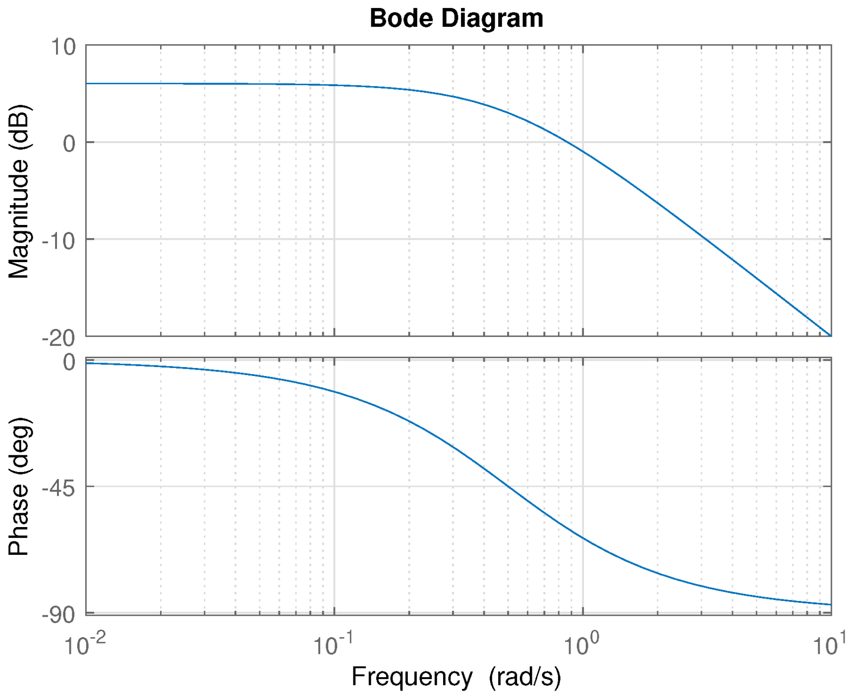
We define the system gain to be the relation between output and input amplitude in a steady-state given by their quotient. For linear systems, ordinary or fractional, the gain is independent of the input amplitude. Therefore, it can be obtained experimentally by introducing sinusoidal signals of unit amplitude with no loss of generality. Depending on input frequency, a different value is obtained. This relation of amplitudes depending on frequency is represented in a magnitude diagram using a log-log scale. See, for instance, Figure 1. In particular, 0 dB means $\left|y\right|/\left|u\right|=1$, i.e., there is neither amplification nor attenuation at the corresponding frequency. The phase diagram represents the phase lag or shift in time resulting between the output and input sinusoidal.

The only significant difference between Bode diagrams corresponding to linear ordinary and linear fractional systems is that for the first ones, asymptotic slopes in the magnitude diagram are integer multiples of 20 dB/dec. In contrast, for fractional systems, we have fractional multiples.

When there are nonlinear phenomena, a new feature appears. The mark of nonlinearity is gain dependence on amplitude. In addition, generally, given a sinusoidal input, the output is no longer a sinusoidal, so Bode diagrams can not be obtained and there is not a superposition principle as the one mentioned above so even if for particular cases an analog of Bode diagrams were obtainable, they would not be of much use. Nevertheless, if such an analog were to exist, it would be useful to know what it would resemble. Fortunately, for a particular class of nonlinear systems, in the convergent systems [29], such an analog exists, at least for the magnitude diagram. Convergent nonlinear (ordinary) systems, when given periodic input, produce a periodic output of the same period again, a property often called input entrainment. This allows for a nonlinear frequency response function that characterizes all steady-state solutions corresponding to harmonic excitations at various amplitudes and frequencies [29], thus extending the conventional frequency response function defined for linear systems. However, as stressed by Pavlov et al. in [29], the gain in the steady-state will not only depend on the frequency, as in the linear case, but also on the excitation amplitude. Consequently, the Bode magnitude diagram is no longer given by a curve but by a surface.

Suppose linear fractional systems were able to generate nonlinear phenomena. In that case, their Bode diagram should show this double dependence on frequency and amplitude and then be given by a surface or, alternatively, a family of curves. The fact that a single curve gives their Bode diagram (for magnitude or phase) visually shows that they are not able to represent nonlinearities. These curves (for the magnitude diagram) can have asymptotic slopes, which are fractional multiples of 20 dB/dec showing fractional systems capture features not represented by ordinary systems. In particular, the non-local phenomena, such as memory effects, are mentioned above.

5. Oustaloup’s Filter Approximation

Due to practical limitations, it is often necessary to approximate a fractional-order operator with a more manageable one of often much higher order, though. Such replacement is the high-order rational approximation of the fractional-order operator, and a standard method to derive it that we will adopt in the paper is due to Oustaloup [30]. Finally, the previous transfer function is approximated by a classical transfer function of integer order [28,31].

Oustaloup’s recursive filter gives a very good approximation of fractional operators in a specified frequency range. It is a well-established method and is often used for practical implementation of fractional-order systems and controllers [32,33]. It is summarized next.

In order to approximate a fractional differentiator of order $\alpha$ or a fractional integrator of order $(-\alpha )$ by a conventional transfer function, one may compute the zeros and poles of the latter using the following equations:

$$s^{\alpha }\approx K\prod _{k=1}^N\frac{s+{\omega }_k^{\prime }}{s+{\omega }_k},$$

(15)

where:

$$\begin{array}{cc}\hfill {\omega }_k^{\prime }& ={\omega }_b·{\omega }_u^{(2k-1-\alpha )/N},\hfill \end{array}$$

(16)

$$\begin{array}{cc}\hfill {\omega }_k& ={\omega }_b·{\omega }_u^{(2k-1+\alpha )/N},\hfill \end{array}$$

(17)

$$\begin{array}{cc}\hfill K& ={\omega }_h^{\alpha },{\omega }_u=\sqrt{{\omega }_h/{\omega }_b},\hfill \end{array}$$

(18)

with ${\omega }_u$ being the unit gain frequency and the central frequency of a band of frequencies geometrically distributed around it. That is, ${\omega }_u=\sqrt{{\omega }_h{\omega }_b}$, ${\omega }_h$, ${\omega }_b$ are the high and low transitional frequencies.

One strong advantage of Oustaloup’s filter is that the amount of necessary computations grows linearly with the order of approximation N. Indeed, only a limited history of the process is considered. The bigger the N, the better the approximation of the differentiator $s^{\alpha }$ in its frequency band.

Besides, we shall remark that it suffices to consider $\alpha \in (0,1)$, since we can always write:

$$s^{\alpha }=s^n{s}^{\gamma },$$

(19)

where $n=\alpha -\gamma$ denotes the integer part of $\alpha$, so that $\gamma \in (0,1)$, since fractional and integer-order derivatives commute for fractional orders $\alpha \ge 1$, and $s^{\gamma }$ is obtained by the Oustaloup approximation by using (15).

Thus, every operator in (13) may be approximated using (19) and replaced by the obtained approximation, yielding as a final result a conventional integer-order transfer function. This suggests that, after all, identifying in the time domain a system with a fractional-order model would lead to substantially the same results as those provided by a classical integer-order model of possibly (very) high order at the price of a significantly larger amount of computations.

6. Fractional-Order Modeling and Control Toolboxes

To perform the calculations and simulations needed to complete our numerical results, we chose to use the MATLAB toolbox FOMCON, developed by Tepljakov [34], which is based on three other popular toolboxes. For further information, we refer the reader to the survey paper by Li et al. [35].

• FOTF (Fractional Order Transfer Function) is a control toolbox for fractional order systems developed by Xue et al. [31,36], which extends many MATLAB built-in functions. The FOTF approximate fractional differential operators by means of a discretization of the Grünwald–Letnikov definition of noninteger derivative, but other approximation methods are possible [36].
• Ninteger (Non-integer) is a toolbox for MATLAB intended to help develop non-integer order controllers for single-input, single-output plants and assess their performance. It was originally developed by Valério and Sá da Costa [37]. It uses integer-order approximations of the fractional-order transfer function, mainly based on Oustaloup’s filter; more generally, the whole toolbox has been inspired by the original CRONE one, from which Ninteger imported several methods.
• CRONE (Commande Robuste d’Ordre Non Entier is a robust command of non-integer order) Toolbox, developed in the nineties by the CRONE team [32]. Many approximation techniques proposed by the CRONE team are considered as foundational in the literature (see e.g., [28,33]). For instance, Oustaloup’s (leader of the CRONE team) method of approximation of transfer functions was one of the cornerstones of the original CRONE toolbox.

FOMCON toolbox for MATLAB is a fractional-order calculus-based toolbox for system modeling and control design. Tepljiakov [33] developed it upon the core of FOTF. Consequently, the main object of analysis in FOMCON is a fractional-order transfer function of the form:

$$G\left(s\right)=\frac{b_m{s}^{{\beta }_m}+b_{m-1}{s}^{{\beta }_{m-1}}+\cdots b_0{s}^{{\beta }_0}}{a_n{s}^{{\alpha }_n}+a_{n-1}{s}^{{\alpha }_{n-1}}+\cdots a_0{s}^{{\alpha }_0}},$$

(20)

and its main aim is to extend conventional control schemes, like PID controllers, with concepts of fractional calculus and provide tools to implement fractional-order systems and controllers.

FOMCON was initially developed in order to facilitate the research of fractional-order systems. This involved writing convenience functions, e.g., the polynomial string parser, and building a GUI. However, a full suite of tools was also desired due to certain limitations in existing toolboxes. Once the core of the basic function of FOMCON was established, it was then extended with advanced features, such as fractional-order system identification and FOPID controller design. This makes the toolbox suitable for both beginners and more demanding, experienced users.

7. Numerical Results

In this section, we present some numerical results on two cases of system identification, the first one coming from experimental data and the second one simulated data. The goal is to investigate whether fractional-orders models, being more flexible than their ordinary integer-order counterparts, are actually more effective in approximating a given nonlinear system and, if that is the case, whether the computational cost to generate them is worth it in real-life scenarios.

Thus, our purpose is to identify a transfer function G as an ordinary, integer-order transfer function and obtain an approximation of the system. Then, we will employ the MATLAB FOMCON toolbox by Tepljakov [33] to identify the systems as fractional-order models, using G as a starting point. In both cases, we simulate the outputs for identification data and validation data, and we parallel them to the experimental data, estimating the error committed as the squared norm of their difference.

Finally, we compare the performance of the fractional-order model against one of the integer-order models, with a particular focus on validation: the concern is that the flexibility of fractional models can cause them to over-fit the identification data, weakening their performance against validation sets.

7.1. Example 1. Experimental Identification of a Furnace

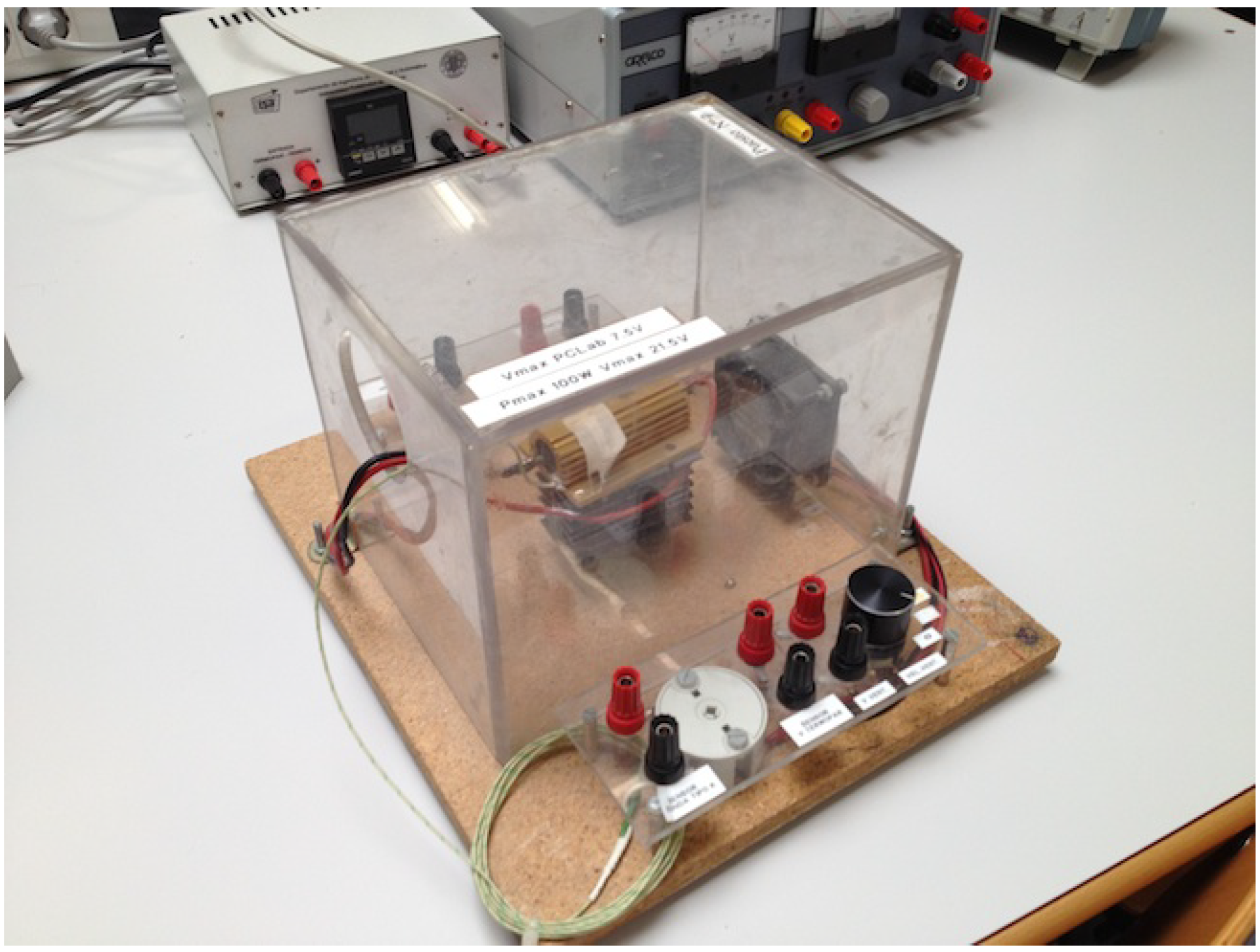
The experimental data are collected from a model furnace used in a lab. It is formed by a power resistor within a plastic box equipped with a fan (see Figure 2). The manipulated variable is the percentage of energy supplied to the resistor, which depends on the applied input voltage. The fan is kept at a constant speed for our experiments. The temperature within the box is measured using a K-type thermocouple calibrated for a temperature range [−50, 250] °C. The system is nonlinear, the gain depends on input amplitude and, besides, it is not the same to raise the temperature or lower it. For control purposes, it is considered to be well approximated by a first-order LTI model. These systems usually have a pure time delay, which is almost negligible in this model.

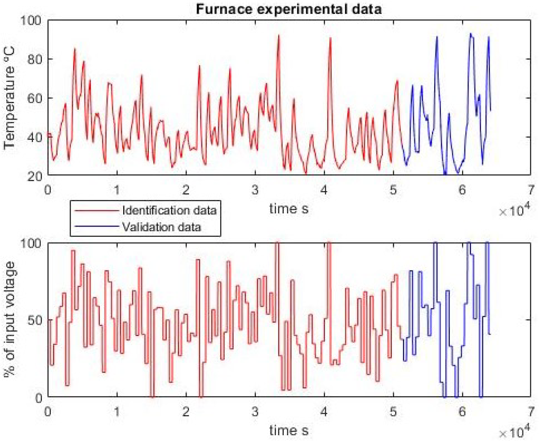
The data set comes in form of a table whose columns are ordered as:

• Time instants in seconds;
• Input u (voltages) in percentage of maximum input voltage;
• Output y (temperatures) in °C.

We chose to divide the data set with an 80:20 split between the identification and validation sets, as can be seen in Figure 3.

7.1.1. Integer-Order Identification

Along this section, the parametric identification develops with fixed orders so that we only estimate the unknown coefficients; in particular, here, in a first instance, G is chosen to be of first-order. In a second step, one pole and one zero are added. The time step is $T_s=12$ s. The resulting first-order transfer function is:

$$G_{I1}\left(s\right)=\frac{0.003192}{s+0.004102}$$

(21)

with a data fit of $65.29\%$. The second-order (with a zero) approximation is:

$$G_{I2}\left(s\right)=\frac{0.003207s-2.166\times {10}^{-8}}{s^2+0.003965s+8.054\times {10}^{-8}}$$

(22)

with a data fit of $70.91\%$. Although it may seem a poor approximation, it is enough for control purposes.

7.1.2. Fractional-Order Identification

The next phase is fractional-order identification with the FOMCON toolbox. The process starts with an initial transfer function: we choose the $G_{Ii}$ we found earlier in (21) and (22) to be the input of the FOMCON function, which optimizes the parameters, including now the exponents. Here, we leave fairly wide freedom of search, setting parameter bounds as low as $-{10}^2$ and as high ${10}^3$, and setting the order of derivation to be in the range [${10}^{-9}$, 10]. Concerning the frequency range, instead, we allow searching in the range of [${10}^{-4}$, ${10}^3$] radians per second.

System identification is an optimization process; we thus need a (nonlinear) optimization algorithm to help us perform it. The FOMCON toolbox gives two options: Levenberg–Marquardt and the Trusted Region Reflective. The second one gives better results. We also assume that the model has static gain. The fractional-order transfer functions obtained are:

$$G_{F1}\left(s\right)=\frac{0.0024}{s^{1.0474}+0.0032}$$

(23)

and:

$$G_{F2}\left(s\right)=\frac{-0.01752s^{1.0577}+0.0684\times {10}^{-4}}{s^{1.8809}+0.1976s^{0.96105}+0.0018}$$

(24)

7.1.3. Validation

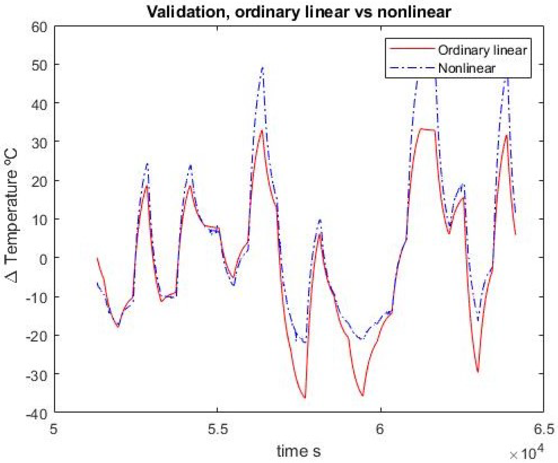
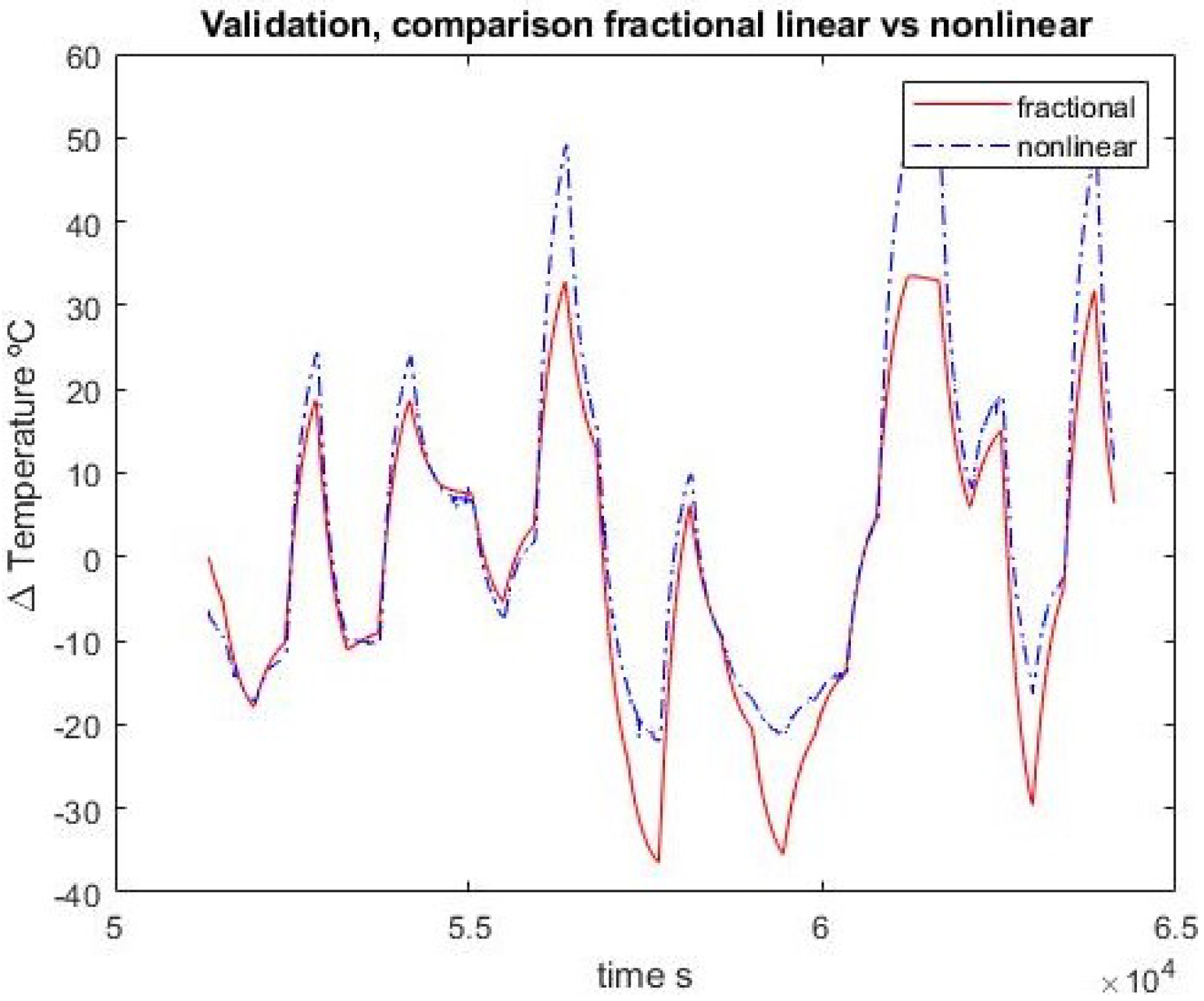
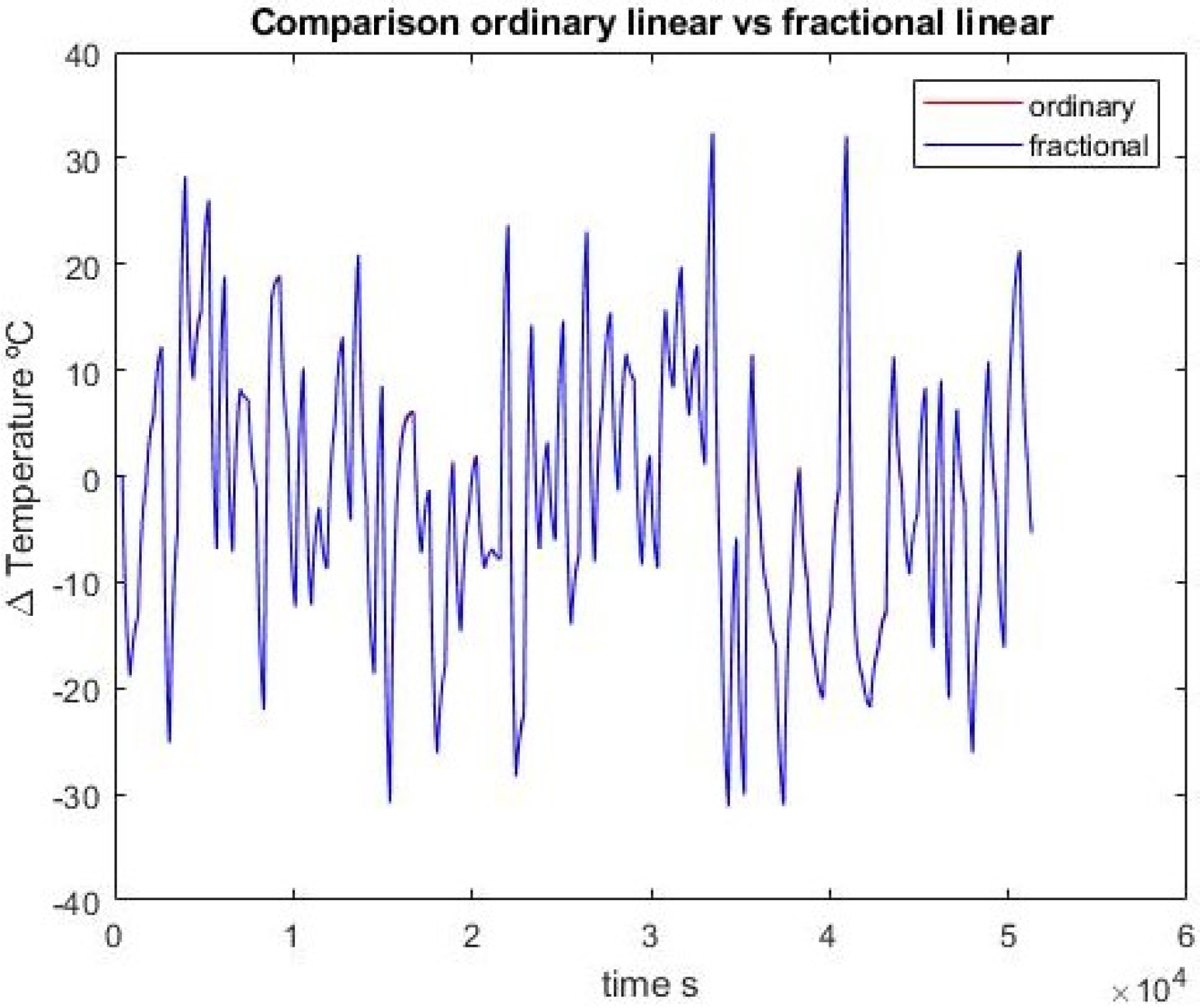
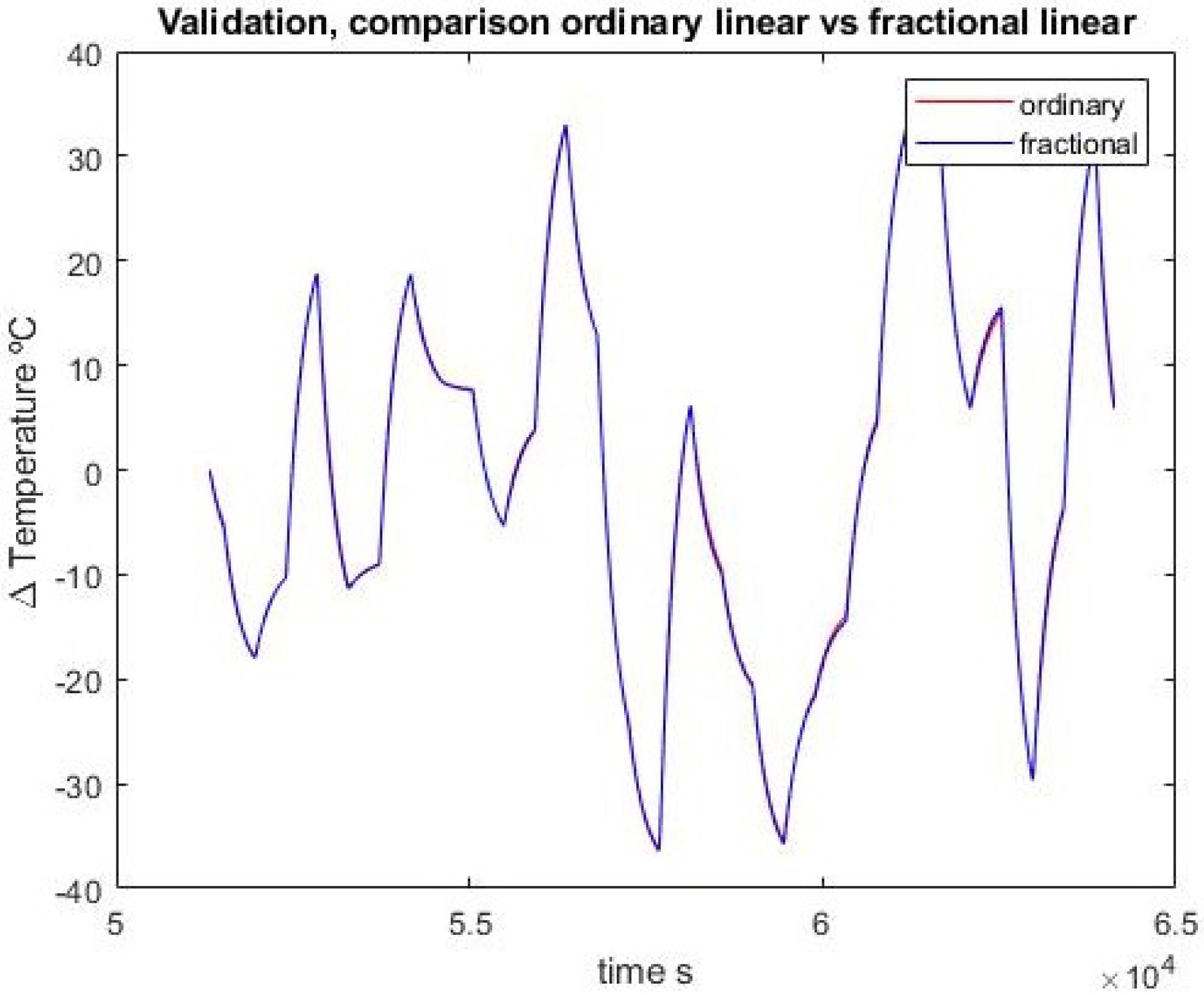
Both the integer and fractional transfer functions are used to simulate data to parallel against the identification and validation sets; the results are discussed next.

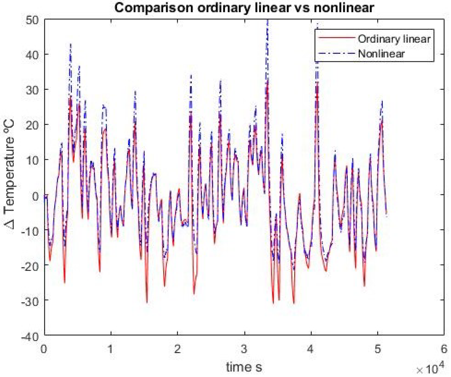
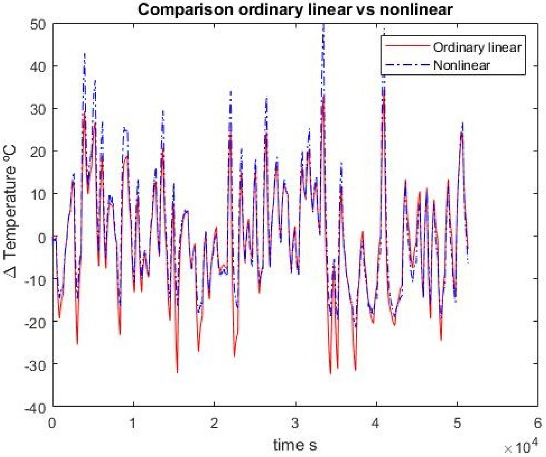
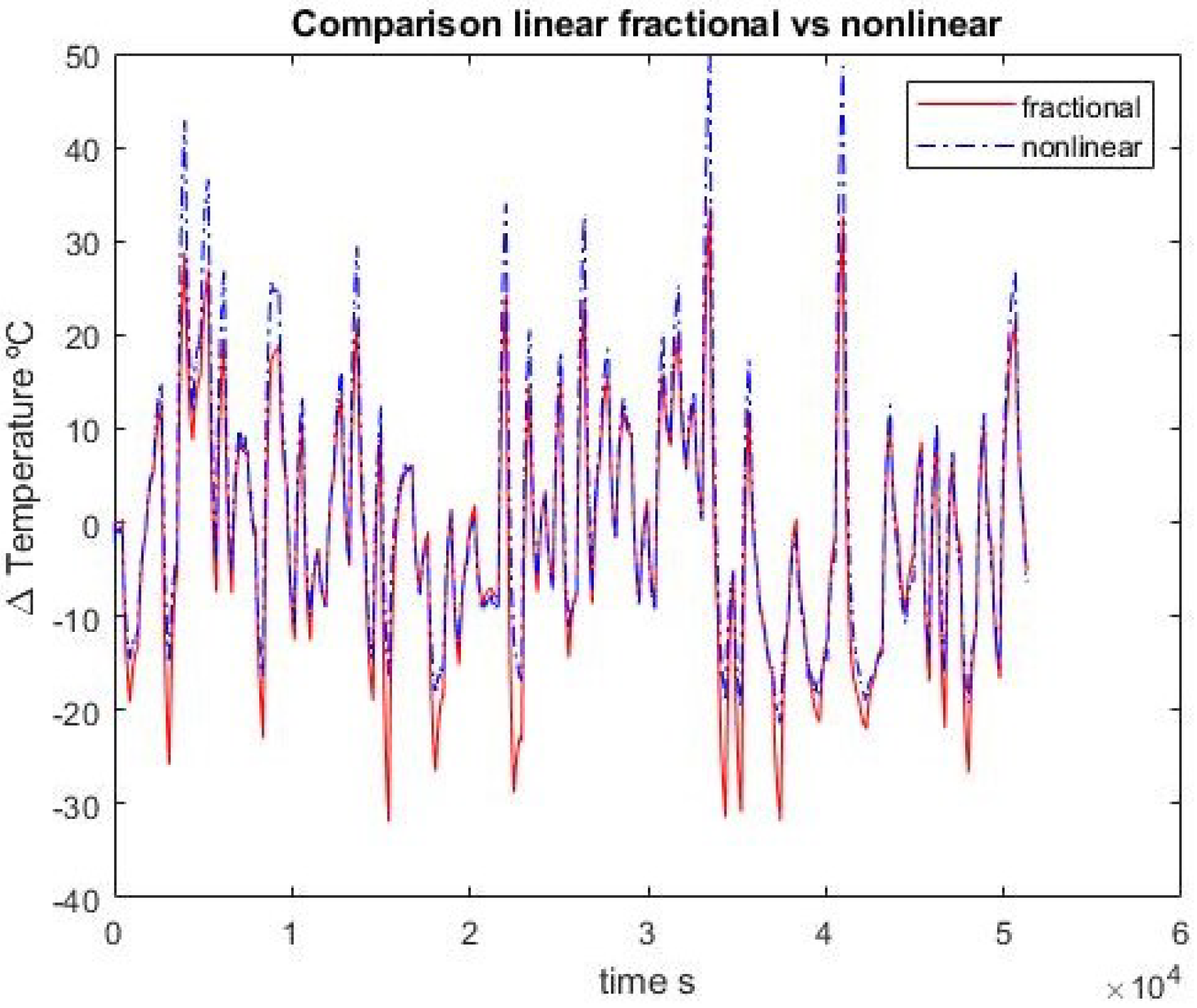
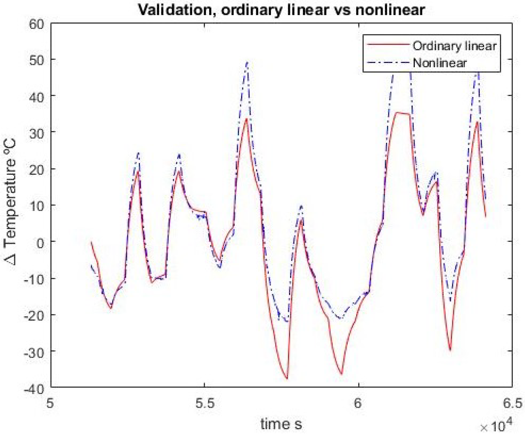
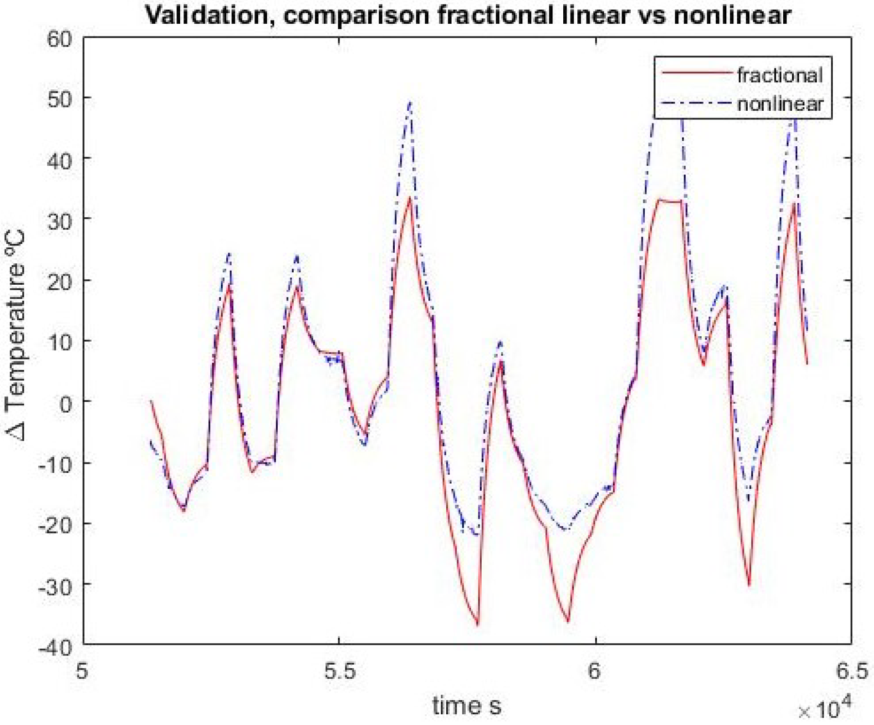
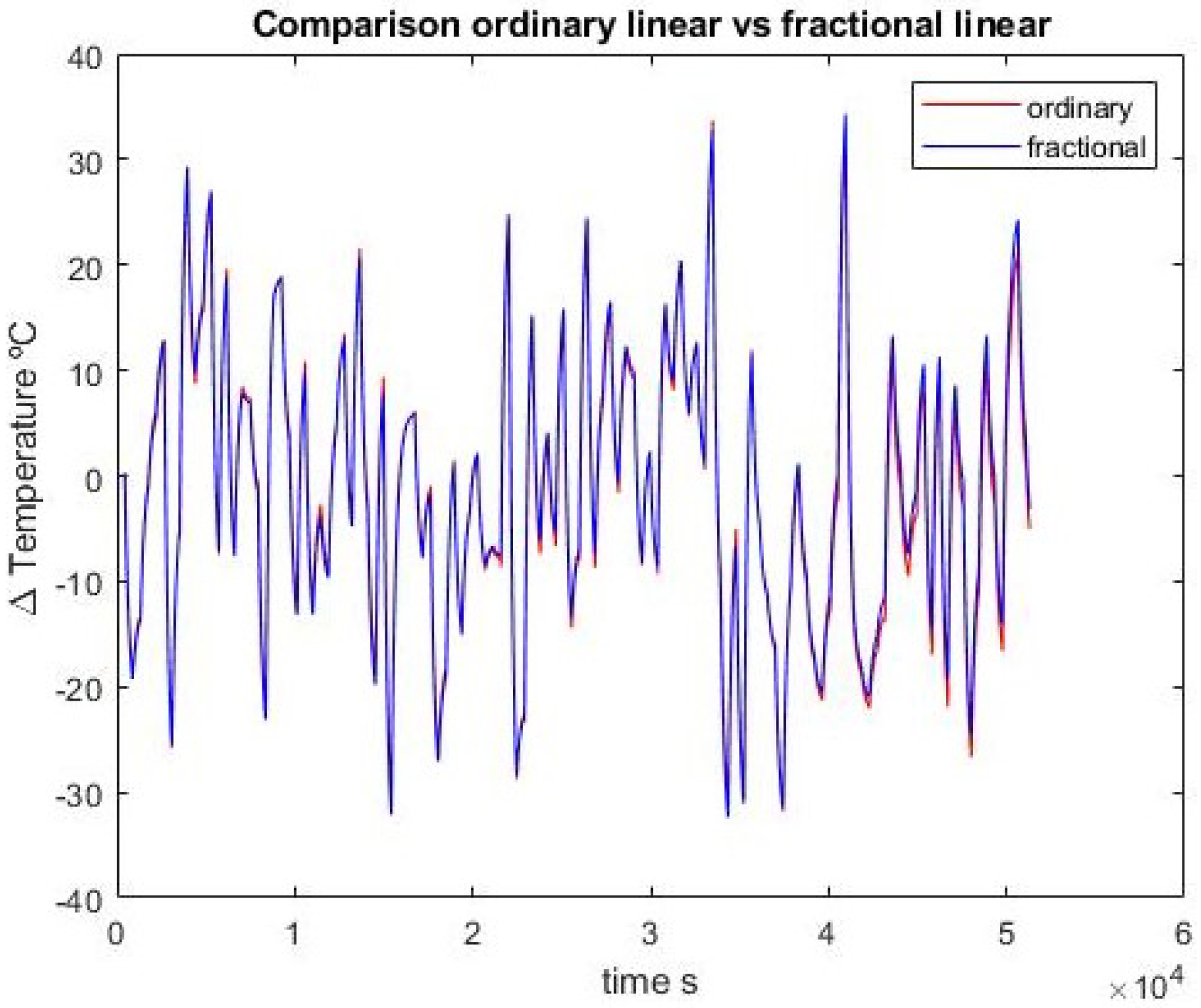
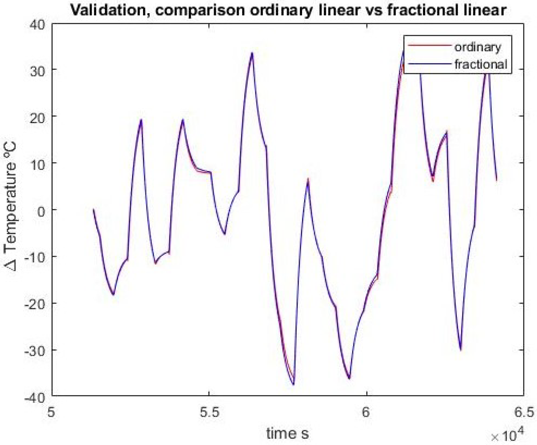
In the first-order case, the fractional order and ordinary approximations are virtually identical. Adding one pole and one zero, the fractional approximation is better with the identification set but the advantage disappears when confronted with validation data. In any case, the results are quite close.

It may also be noted that the first-order integer model has two parameters and the second-order one has four. The corresponding fractional models have three and seven, respectively. So a fairer test would be between the first fractional model with three parameters and the second-order integer model with four. In this case, the fractional model does not outperform the integer one.

Table 2. Furnace approximation errors. Computed as $\parallel y-\tilde{y}\parallel$, where y are the experimental data, $\tilde{y}$ are the approximated data and $\parallel ·\parallel$ is the Euclidean norm. The relative percentage expresses the difference between the errors committed by the two models in a proportion of the highest.

	Identification Error			Validation Error
TF Order	Integer	Fractional	Relative %	Integer	Fractional	Relative %
1st	$302.26$	$302.5$	$0.08$%	$244.26$	$244.28$	$0.006$%
2nd	$302.12$	$298.68$	$1.14$%	$235.46$	$243.51$	$3.3$%

reports the errors committed, expressed as the norm of the difference between approximated and experimental data.

Figure 4, Figure 5, Figure 6, Figure 7, Figure 8 and Figure 9 show the comparison between the ordinary model and the fractional one for the first-order approximation, with respect to experimental data of both identification and validation sets, and between each other. Figure 10, Figure 11, Figure 12, Figure 13, Figure 14 and Figure 15 show the comparison between the ordinary model and the fractional one for the second-order approximation

7.2. Example 2. Identification of a Simulated Fractional Model

This academic example partially replicates example 6.1 from [38]. There, a system description is given by the transfer function.

$$G\left(s\right)=\frac{-1.3333s^{0.63}+2.6667}{1.3333s^{3.501}+2.5333s^{2.42}+1.7333s^{1.798}+1.6667s^{1.31}+1}.$$

(25)

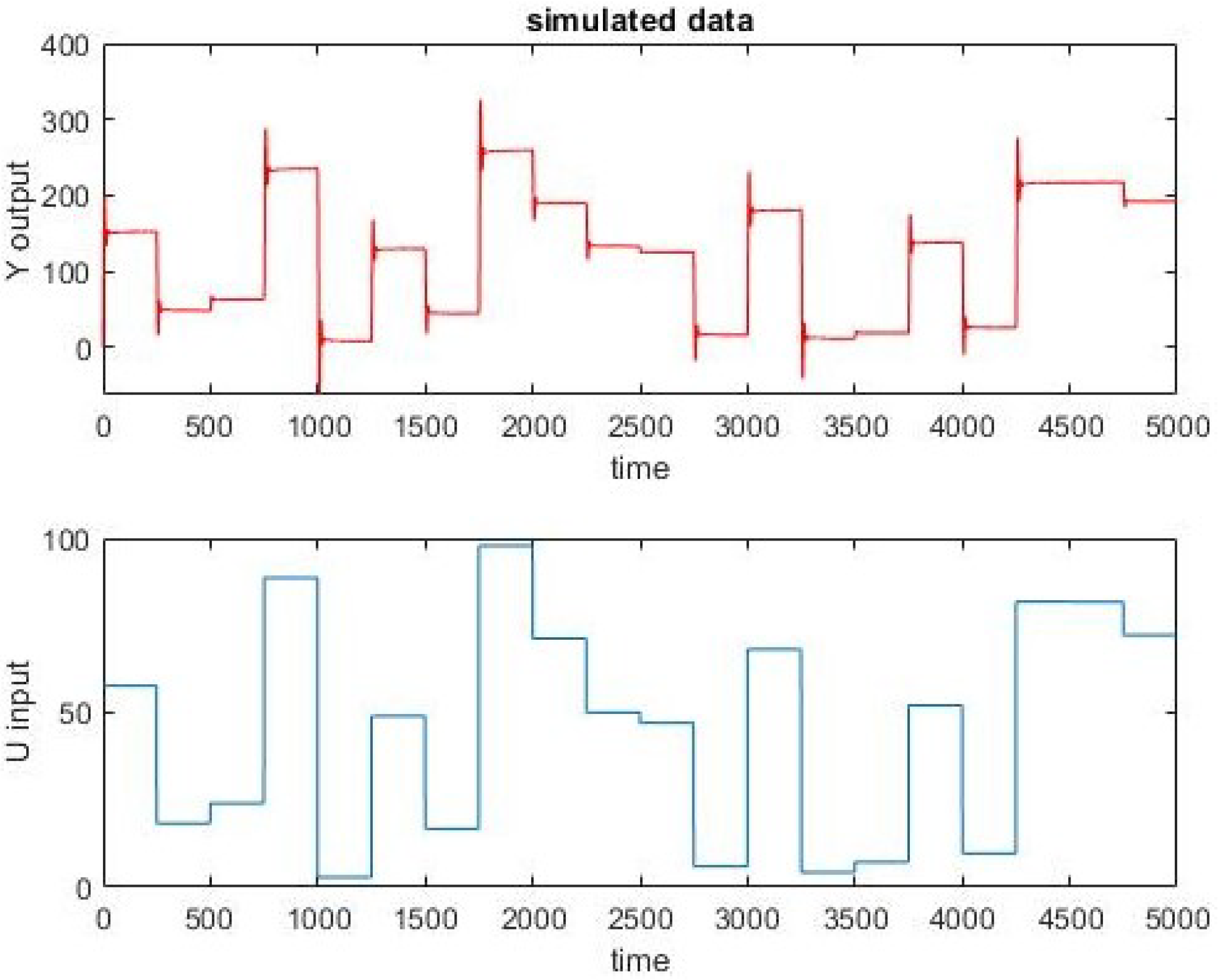
with a strong fractional character, i.e., such that its exponents are not close to integer numbers. Then, in order to illustrate the use of the fid function for fractional identification in the FOMCON toolbox, input-output data are obtained (see Figure 16) and a fractional order transfer function is identified. Starting from:

$$G_0\left(s\right)=\frac{s+1}{s^3+s^{2.5}+s^{1.5}+s+1}.$$

(26)

as an initial guess, the obtained function is:

$$G_F\left(s\right)=\frac{-1.281s^{0.656}+2.657}{1.396s^{3.495}+2.145s^{2.471}+2.736s^{1.817}+1.199s^{1.176}+1}.$$

(27)

with a $99.98\%$ fit. Here, an integer order transfer function with the same number of parameters is identified instead. Afterward, Oustaloup’s and Matsuda’s approximations for (25) are obtained, and the different Bode diagrams are compared.

7.2.1. Integer-Order Identification

The following integer order transfer function with 11 parameters, as in (25), is obtained using the tfestim function from Matlab:

$$G_I\left(s\right)=\frac{15.63s^4+4.076s^3+0.1355s^2+0.0008051s+8.178\times {10}^{-7}}{s^6+24.38s^5+8.618s^4+1.644s^3+0.05196s^2+0.0003044s+3.07\times {10}^{-7}}.$$

(28)

The quality of the approximation is very high, with a fit percentage of $99.84\%$ with respect to the input-output data in Figure 16, close to that of the identified fractional model (27). This fact shows that an integer-order transfer function can approximate, within a given frequency range, data generated by a fractional-order one with very high precision without the need for excessively high order of derivation or computational resources.

7.2.2. Oustaloup’s and Matsuda’s Filters

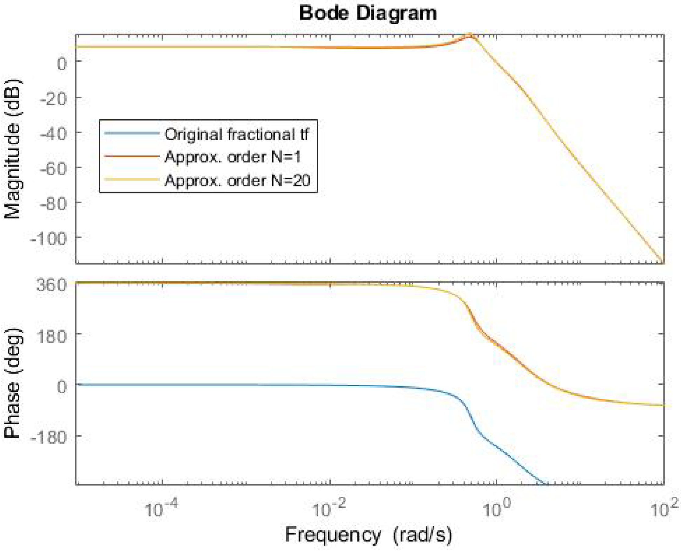
Finally, the Oustaloup’s and Matsuda’s filters are obtained to approximate (25). For the first one, the function oustapp from the FOMCON toolbox is used. We set the coefficients to be bounded in [${10}^{-3}$, 10${}^3$] and the order of approximation to be equal to $N=20$. Oustaloup’s approximation is quite cumbrous, too much to report it here; it suffices to say that it has 262 terms. A significant reduction can be obtained by reducing the order of approximation in the Oustaloup method. Nevertheless, even reduced to the minimum $N=1$, the default is $N=5$, a transfer function with 18 poles and 15 zeroes is obtained. The bode diagrams of both approximations are very close both for magnitude and phase, as seen in Figure 17, where they are also compared with the Bode diagram for the original fractional transfer function (25).

Looking for a still more reduced approximation, Matsuda’s filter was programmed following [31]. In this case, the order of the resulting transfer function can be easily controlled. In a first step, a first-order approximation is obtained:

$$G_m\left(s\right)=\frac{-0.1365s+1.377}{s+0.4063}.$$

(29)

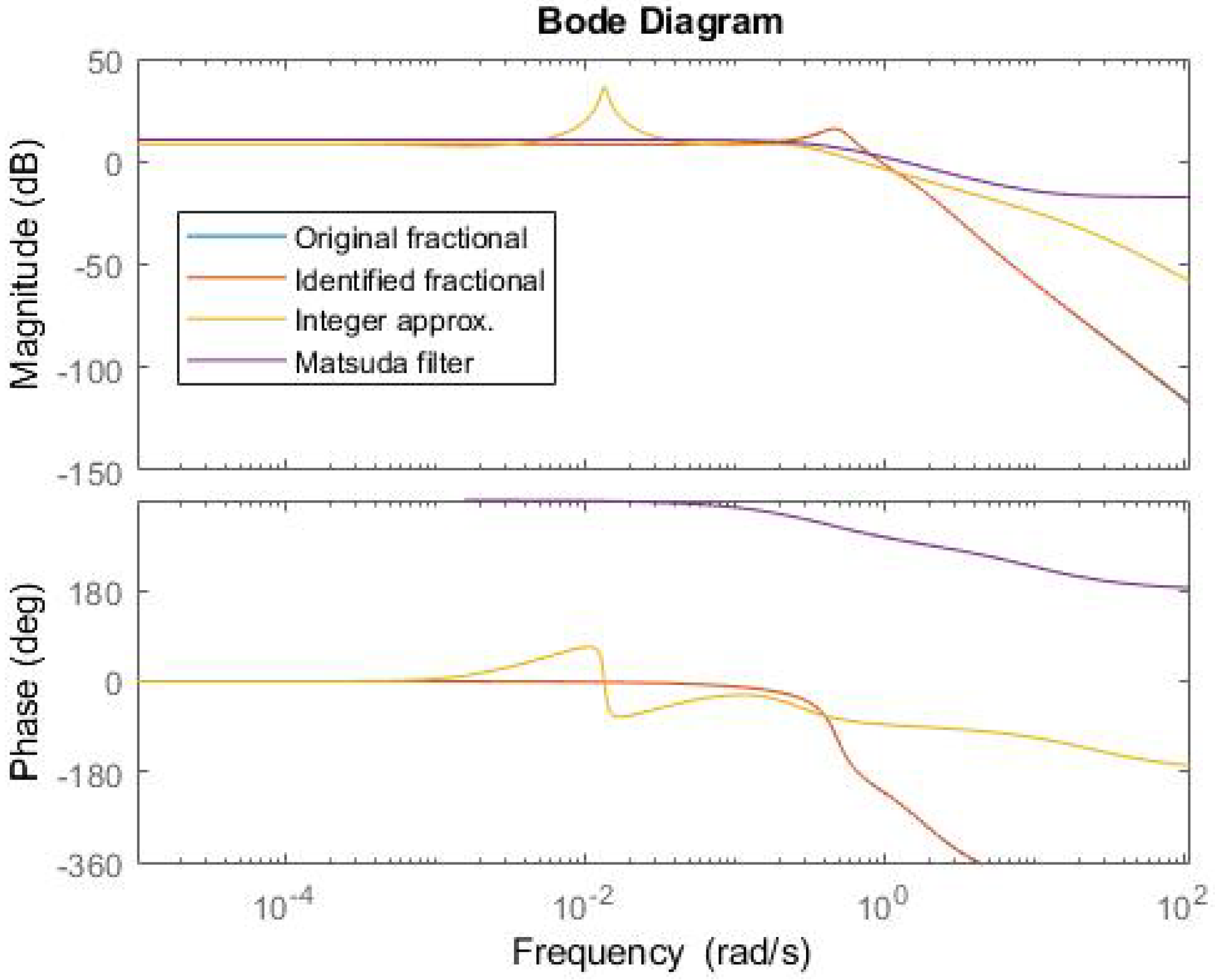
In Figure 18, the corresponding Bode diagram is shown only for the order 1 stable filter obtained. Higher-order Matsuda filters approximate much better the magnitude diagram but turn out to be unstable and consequently not valid.

In Figure 18, the Bode diagrams for the original transfer function (25), the identified one (27), the integer order approximation (28) and the Matsuda filter (29), are compared.

8. Conclusions

Fractional-order operators have been gaining popularity in Control Engineering in recent years. They are highly promising for dealing with non-local phenomena; in addition, fractional techniques have been used in a wide range of applications to all kinds of systems, including nonlinear ones. However, a comparison of the Bode diagrams for linear ordinary, linear fractional, and convergent systems leads to the question of whether any nonlinearity can be captured simply by using fractional operators. Still, in the same way, a linear ordinary one can approximate a nonlinear system, linear fractional systems can also be used as an approximation.

In the experimental case examined in this work, fairly wide freedom was given to parameter search in order to give a chance to fractional operators to show their strength at their best. However, fractional-order identification of transfer function failed to provide significant improvements with respect to the performance of standard integer-order identification.

Randomly generated data also confirmed this trend when they were used to simulate outputs based on a fractional transfer function. A relatively low-order integer transfer function obtained using classic standard methods was very effective in fitting the data for low and medium frequencies, the Oustaloup’s approximation giving a big transfer function even setting the method approximation order to the minimum and Matsuda’s one presenting problems of instability.

In conclusion, these results suggest fractional order methods naturally outperform classical ones when treating phenomena, such as memory effects and non-local behavior in general. However, when applying them to nonlinear systems, this advantage vanishes. For the implementation phase, the use of ordinary linear approximations, such as Oustaloup’s and Matsuda’s, reinforces the situation. In the end, an ordinary system is used; already standard methods could have obtained that.

References

- Podlubny, I. Geometric and physical Interpretation of fractional Integration and fractional differentiation. Fract. Calc. Appl. Anal. 2002, 5, 367–386. [Google Scholar]
- Tarasov, V. Geometric interpretation of fractional-order derivative. Fract. Calc. Appl. Anal. 2016, 19, 1200–1221. [Google Scholar] [CrossRef]
- Valerio, D.; Ortigueira, M.D.; Lopes, A.M. How many fractional derivatives are there? Mathematics 2022, 10, 737. [Google Scholar] [CrossRef]
- Ortigueira, M.D.; Machado, J.T. What is a fractional derivative? J. Comput. Phys. 2015, 293, 4–13. [Google Scholar] [CrossRef]
- Ortigueira, M.; Machado, J.T. Which derivative? Fractal Fract. 2017, 1, 3. [Google Scholar] [CrossRef]
- Tarasov, V.E.; Tarasova, S.S. Fractional derivatives and integrals: What are they needed for? Mathematics 2020, 8, 164. [Google Scholar] [CrossRef] [Green Version]
- Baleanu, D.; Güvenç, Z.B.; Machado, J.A.T. New Trends in Nanotechnology and Fractional Calculus Applications; Springer: Berlin/Heidelberg, Germany, 2010; Volume 10. [Google Scholar]
- Atangana, A. Derivative with a New Parameter: Theory, Methods and Applications; Academic Press: Cambridge, MA, USA, 2015. [Google Scholar]
- Sun, H.G.; Zhang, Y.; Baleanu, D.; Chen, W.; Chen, Y.Q. A new collection of real world applications of fractional calculus in science and engineering. Commun. Nonlinear Sci. Numer. Simulat. 2018, 64, 213–231. [Google Scholar] [CrossRef]
- Fuente, D.; Lizama, C.; Urchueguía, J.F.; Conejero, J.A. Estimation of the light field inside photosynthetic microorganism cultures through Mittag-Leffler functions at depleted light conditions. J. Quant. Spectrosc. Radiat. Transf. 2018, 204, 23–26. [Google Scholar] [CrossRef]
- İlhan, E.; Kıymaz, İ.O. A generalization of truncated M-fractional derivative and applications to fractional differential equations. Appl. Math. Nonlinear Sci. 2020, 5, 171–188. [Google Scholar] [CrossRef] [Green Version]
- Lewandowski, M.; Orzyłowski, M. Fractional-order models: The case study of the supercapacitor capacitance measurement. Bull. Pol. Acad. Sci.-Tech. 2017, 65, 449–457. [Google Scholar] [CrossRef] [Green Version]
- Feliu-Batlle, V.; Rivas-Perez, R.; Castillo-García, F. Simple fractional order controller combined with a Smith predictor for temperature control in a steel slab reheating furnace. Int. J. Control Autom. Syst. 2013, 11, 533–544. [Google Scholar] [CrossRef]
- Xue, D.; Zhao, C.; Chen, Y. Fractional order PID control of a DC-motor with elastic shaft: A case study. In Proceedings of the 2006 American Control Conference, Minneapolis, MN, USA, 14–16 June 2006; p. 6. [Google Scholar] [CrossRef]
- Acay, B.; Inc, M. Electrical circuits RC, LC, and RLC under generalized type non-local singular fractional operator. Fractal Fract. 2021, 5, 9. [Google Scholar] [CrossRef]
- Zhang, L.; Kartci, A.; Elwakil, A.; Bagci, H.; Salama, K. Fractional-order inductor: Design, simulation, and implementation. IEEE Access 2021, 9, 73695–73702. [Google Scholar] [CrossRef]
- Hao, C.; Wang, F. Design method and implementation of the fractional-order inductor and its application in series-resonance circuit. Int. Circuit Theory Appl. 2022, 50, 1400–1419. [Google Scholar] [CrossRef]
- Jamil, A.; Tu, W.; Ali, S.; Terriche, Y.; Guerrero, J. Fractional-order PID controllers for temperature control: A review. Energies 2022, 15, 3800. [Google Scholar] [CrossRef]
- Rong, C.; Zhang, B.; Jiang, Y. Analysis of a fractional-order wireless power transfer system. IEEE Trans. Circuits Syst. II Express Briefs 2020, 67, 1755–1759. [Google Scholar] [CrossRef]
- Tian, J.; Xiong, R.; Shen, W.; Wang, J.; Yang, R. Online simultaneous identification of parameters and order of a fractional order battery model. J. Clean. Prod. 2020, 247, 119147. [Google Scholar] [CrossRef]
- Wang, S.F.; Ye, A. Dynamical Properties of Fractional-Order Memristor. Symmetry 2020, 12, 437. [Google Scholar] [CrossRef] [Green Version]
- Tarasov, V. No nonlocality. No fractional derivative. Commun. Nonlinear Sci. Numer. Simulat. 2018, 62, 157–163. [Google Scholar] [CrossRef] [Green Version]
- Podlubny, I. Fractional Differential Equations; Academic Press: Cambridge, MA, USA, 1999. [Google Scholar]
- Garrappa, R. Numerical solution of fractional differential equations: A survey and a software tutorial. Mathematics 2018, 6, 16. [Google Scholar] [CrossRef] [Green Version]
- Caputo, M.; Mainardi, F. Linear models of dissipation in anelastic solids. La Rivista del Nuovo Cimento 1971, 1, 161–198. [Google Scholar] [CrossRef]
- Caputo, M.; Mainardi, F. A new dissipation model based on memory mechanism. Pure Appl. Geophys. 1971, 91, 134–147. [Google Scholar] [CrossRef]
- Rabotnov, Y.N.; Leckie, F.A.; Prager, W. Creep problems in structural members. J. Appl. Mech. 1970, 37, 249. [Google Scholar] [CrossRef]
- Monje, C.; Chen, Y.; Vinagre, B.; Xue, D.; Feliu, V. Fractional-Order Systems and Controls: Fundamentals and Applications; Advances in Industrial Control; Springer: Berlin/Heidelberg, Germany, 2010. [Google Scholar]
- Pavlov, A.; van de Wouw, N.; Nijmeijer, H. Frequency response functions and Bode plots for nonlinear convergent systems. In Proceedings of the 45th IEEE Conference on Decision and Control, San Diego, CA, USA, 13–15 December 2006; pp. 3765–3770. [Google Scholar] [CrossRef]
- Oustaloup, A.; Levron, F.; Mathieu, B.; Nanot, F. Frequency-band complex noninteger differentiator: Characterization and synthesis. IEEE Trans. Circuits Syst. I Fundam. Theory Appl. 2000, 47, 25–39. [Google Scholar] [CrossRef]
- Xue, D. Fractional-Order Control Systems: Fundamentals and Numerical Implementations; De Gruyter: Berlin, Germany, 2017. [Google Scholar] [CrossRef]
- Oustaloup, A.; Melchior, P.; Lanusse, P.; Cois, O.; Dancla, F. The CRONE toolbox for MATLAB—CACSD. In Proceedings of the IEEE International Symposium on Computer-Aided Control System Design (Cat. No.00TH8537), Anchorage, AK, USA, 25–27 September 2000; pp. 190–195. [Google Scholar] [CrossRef]
- Tepljakov, A.; Petlenkov, E.; Belikov, J. FOMCON: A MATLAB toolbox for fractional-order system identification and control. Int. J. Microelectron. Comput. Sci. 2011, 2, 51–62. [Google Scholar]
- FOMCON. Toolbox Reference Manual. Available online: http://docs.fomcon.net (accessed on 16 June 2022).
- Li, Z.; Liu, L.; Dehghan, S.; Chen, Y.; Xue, D. A review and evaluation of numerical tools for fractional calculus and fractional order control. Int. J. Control. 2015, 90, 1165–1181. [Google Scholar] [CrossRef] [Green Version]
- Chen, Y.Q.; Petras, I.; Xue, D. Fractional order control—A tutorial. In Proceedings of the 2009 American Control Conference, St. Louis, MO, USA, 10–12 June 2009; pp. 1397–1411. [Google Scholar] [CrossRef]
- Valério, D.; Sá Da Costa, J. Ninteger: A non-integer control toolbox for MATLAB. In Proceedings of the First IFAC Workshop on Fractional Differentiation and Its Application, Bordeaux, France, 19–21 July 2004. [Google Scholar]
- Tepljakov, A. Fractional-Order Modeling and Control of Dynamic Systems. Ph.D. Thesis, Tallinn University of Technology, Tallinn, Estonia, 2017. [Google Scholar]
Figure 1.
Example of a Bode diagram corresponding to an ordinary linear system.
Figure 2.
Model furnace.
Figure 3.
Furnace experimental data for identification and validation.
Figure 4.
First-order linear ordinary model. Identification.
Figure 5.
First fractional-order model. Identification.
Figure 6.
First-order linear ordinary model. Validation.
Figure 7.
First fractional-order model. Validation.
Figure 8.
First-order models comparison with identification data.
Figure 9.
First-order models comparison with validation data.
Figure 10.
Second-order linear ordinary model. Identification.
Figure 11.
Second fractional-order model. Identification.
Figure 12.
Second-order linear ordinary model. Validation.
Figure 13.
Second fractional-order model. Validation.
Figure 14.
Second-order models comparison with identification data.
Figure 15.
Second-order models comparison with validation data.
Figure 16.
Simulated data with the original fractional transfer function.
Figure 17.
Comparison of Bode diagrams for the Oustaloup filters.
Figure 18.
Comparison of Bode diagrams for the integer order approximation and Matsuda’s filter.