Improving the Performance of MapReduce for Small-Scale Cloud Processes Using a Dynamic Task Adjustment Mechanism

Abstract

The MapReduce architecture can reliably distribute massive datasets to cloud worker nodes for processing. When each worker node processes the input data, the Map program generates intermediate data that are used by the Reduce program for integration. However, as the worker nodes process the MapReduce tasks, there are differences in the number of intermediate data created, due to variation in the operating-system environments and the input data, which results in the phenomenon of laggard nodes and affects the completion time for each small-scale cloud application task. In this paper, we propose a dynamic task adjustment mechanism for an intermediate-data processing cycle prediction algorithm, with the aim of improving the execution performance of small-scale cloud applications. Our mechanism dynamically adjusts the number of Map and Reduce program tasks based on the intermediate-data processing capabilities of each cloud worker node, in order to mitigate the problem of performance degradation caused by the limitations on the Google Cloud platform (Hadoop cluster) due to the phenomenon of laggards. The proposed dynamic task adjustment mechanism was compared with a simulated Hadoop system in a performance analysis, and an improvement of at least 5% in the processing efficiency was found for a small-scale cloud application.

1. Introduction

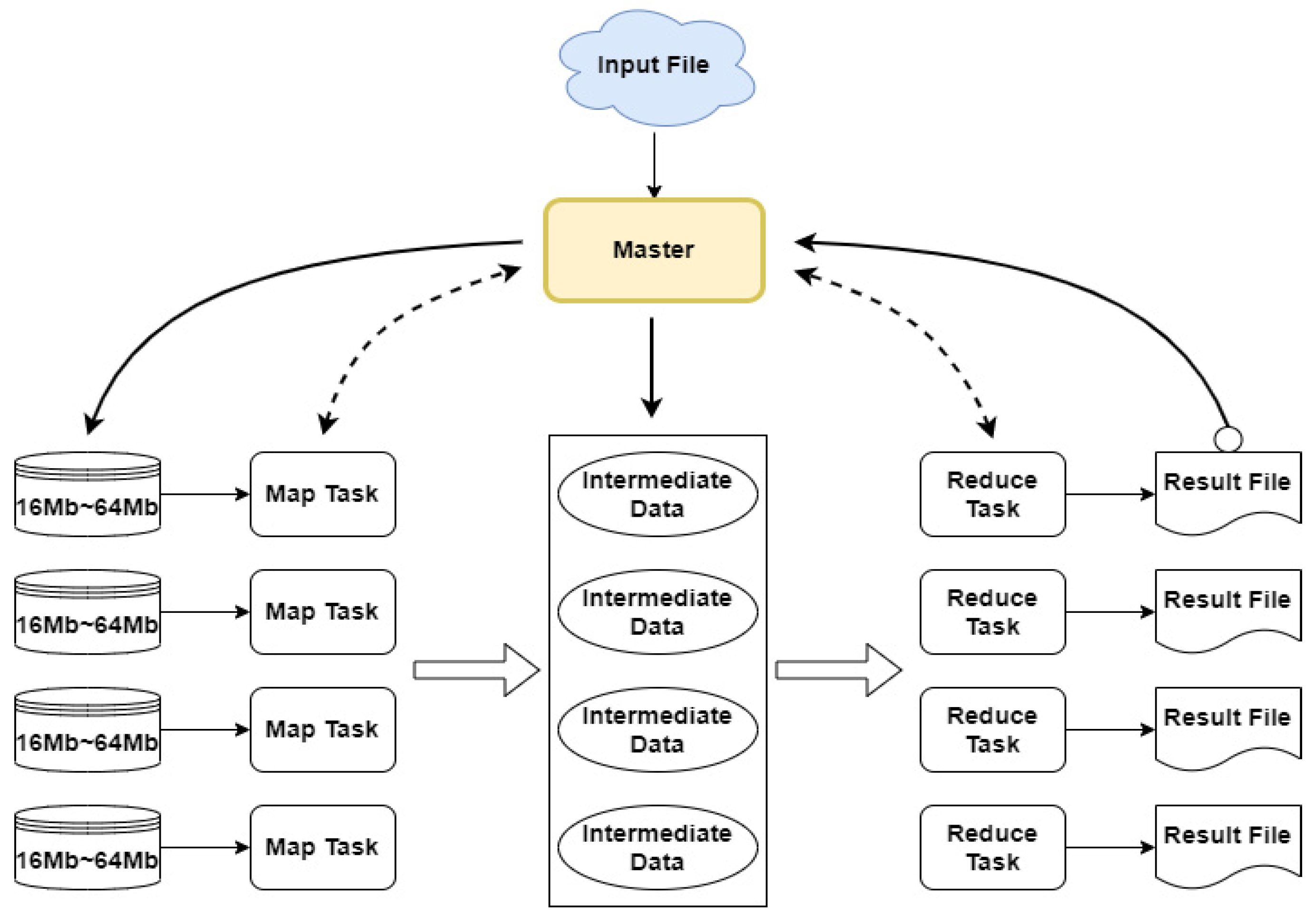
In view of the rapid progress and vigorous development of decentralised parallel processing technology, the Hadoop MapReduce framework proposed by Google has gradually become the basic architecture of cloud computing [1,2,3]. Since it benefits from the advantages of cloud computing technology in terms of dispersing a load for processing by multiple computers, it can be used to realise massive data analysis [4,5,6]. The cloud architecture based on the MapReduce framework is shown in Figure 1. Its operating principle is derived from the distributed parallel computing technology. Multiple computers cooperatively perform a large amount of data calculation for a specific target at the same time in order to realize a high-efficiency calculation amount dispersion function. A cloud architecture running the MapReduce framework uses a master node to control the decentralised operation and to manage multiple slave nodes, in order to process huge numbers of data in a collaborative way. In a MapReduce cloud architecture system, slave nodes are controlled to allow them to execute tasks involving the Map and Reduce functions. The slave nodes execute a fixed number of Map tasks in order to process the input data, generate intermediate data and then execute a fixed number of Reduce tasks to unify the resulting information. When the main node obtains the cloud computing task from the client, it assigns priorities based on the number of idle Map tasks and then allocates some input data to the slave nodes to facilitate the generation of intermediate data. When a slave node executes a Reduce task, it obtains the intermediate data from the corresponding slave node, and, finally, the main node integrates the data from each slave node and processes the intermediate data to give a result in the form of information.

Because each cloud application has a different algorithm, after running the Map task to process the input data, different types and quantities of intermediate data are generated to potentially affect the data transmission time of the runtime system and the computing performance of the slave node. If one of the slave nodes in the small-scale MapReduce cloud architecture receives a large number of intermediate data or the data type is more complex, resulting in a long computing time, this phenomenon is called the intermediate-data skew problem in the MapReduce cloud architecture. Therefore, differences in the type and quantity of intermediate data affect the performance of the slave nodes in terms of performing the Reduce task, resulting in the problem of skew in the intermediate data, which affects the processing efficiency of the MapReduce cloud architecture [7,8,9,10].

The problem of stragglers can also reduce the processing performance of this architecture. When the cloud computing task imposed by the client involves uneven input data, most of the slave nodes complete their portions of the work and then need to wait for the remaining ones, which causes delays. Due to the limited number of slave nodes in the small-scale MapReduce cloud architecture, utilizing the computing resources of idle slave nodes that have completed their work greatly improves the overall MapReduce cloud architecture processing efficiency. Solving the problem of intermediate-data skew is especially important in small-scale MapReduce cloud architectures. In order to solve the problem of intermediate-data skew, studies in the related literature have used load balancing methods [11], and some works have used the slave nodes to process skewed data in order to improve performance [12]. The contributions of this paper are as follows:

• In this paper, we propose an algorithm called Dynamic Task Adjustment Mechanism (DTAM) with Intermediate-Data Processing Cycle Prediction (IDPCP) to improve the processing efficiency;
• Our approach predicts the number of intermediate data that are to be generated by each slave node in the future and dynamically adjusts the number of Map and Reduce tasks assigned to the slave nodes in order to avoid the problem of performance decline due to stragglers;
• Our adjustment mechanism also avoids exceeding the limit on the number of tasks set by the manager in each slave node. The proposed DTAM was compared with the simulated Hadoop (Google Cloud platform) system for a processing efficiency analysis. The experimental results show that at least 5% of the performance efficiency can be improved.

The rest of this paper is organized as follows: The first section of this paper introduces the motivation for this research work. The second section of this paper discusses works in the literature that have focused on solving the problem of intermediate-data skew; the third section describes the operational details of the DTAM with IDPCP; and the fourth section describes the implementation details for small-scale cloud applications. The fifth section carries out an analysis of the effectiveness of the proposed system framework and presents a comparison with a scheme in the literature. Finally, the sixth section summarises the paper.

2. Related Work

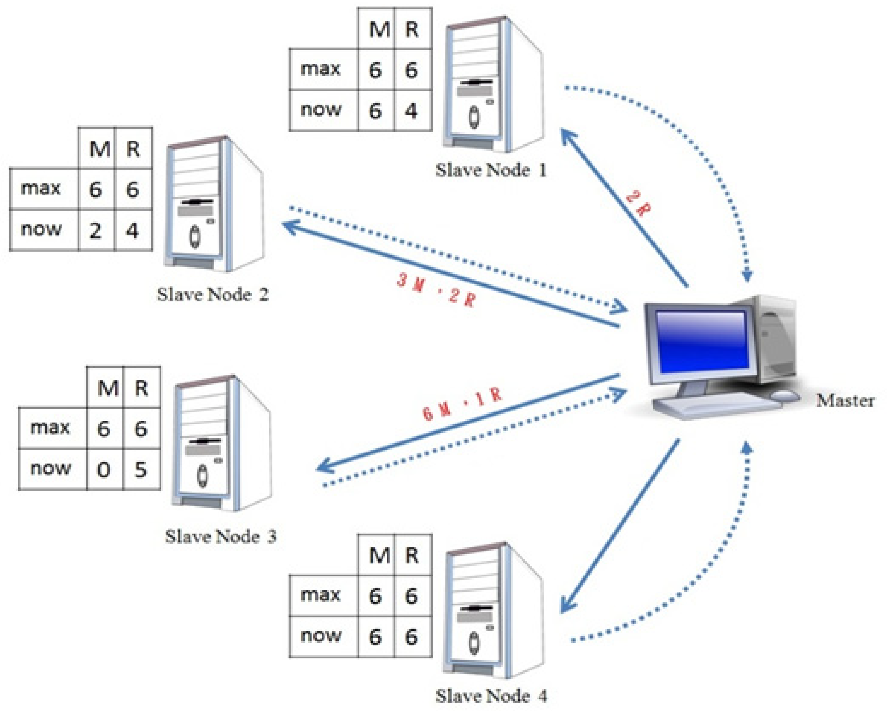
We use a traditional small-scale cloud architecture running the MapReduce software framework as an example. It has one master node and four slave nodes, as shown in Figure 2. In this schedule allocation scheme, each slave node periodically reports the Map and Reduce operations to the master node. At the point shown in the figure, the master node knows that Slave Node 2 has four available Map tasks, while Slave Node 3 has six. The master node, therefore, gives priority to the unprocessed input-data files for Slave Node 3 to process. At the same time, the master node knows that Slave Node 1 has two available Reduce tasks, Slave Node 2 has two and Slave Node 3 has one; therefore, it notifies the slave node with available Reduce tasks to process intermediate-data files. Each slave node running the MapReduce framework traditionally has limits on the maximum numbers of Map and Reduce tasks that can be run, in order to prevent the numbers of tasks exceeding the computer processing load. If the number of intermediate data to be processed in the Reduce task by Slave Node 4 causes it to lag behind the other slave nodes, the problem of intermediate-data skew occurs.

Works in the related literature [13] have proposed the use of support vector machines for performance prediction to solve the problem of intermediate-data skew and to avoid the problem of performance degradation caused by using only the hashing function to allocate intermediate data to the Reduce task. This approach also avoids skew in the input intermediate data of the Map task and uses virtual segmentation technology to divide the area. One proposal in the literature used machine learning to predict abnormal performance in the Reduce task by the slave nodes. It used a heterogeneity-aware partition algorithm to divide a Map task with a large number of input intermediate data and then implemented a load balancing process to solve the problem of intermediate-data skew. However, this scheme only dealt with abnormal performance of the slave nodes. The DTAM algorithm proposed in this paper predicts the workload for all the slave nodes in a small-scale cloud architecture to avoid the problem of delay in response times.

Another prior study [12] discussed the problem of performance degradation caused by delays in the network transmission of intermediate data and used intermediate-data-type perception to determine the network transmission requirements between the slave nodes that processed Map and Reduce tasks. A communication-oriented Reduce assignment method was used to decrease the network transfer time in order to solve the problem of intermediate-data skew. Since the intermediate data generated from a given Map task may not necessarily be used to execute the Reduce task on the same slave node, the network transmission of the intermediate data must be performed between different slave nodes. If this network transmission operation is relatively large, the efficiency drops. One approach in the literature applied type awareness to Map tasks with the aim of allocating the same slave nodes to process the Reduce tasks, in order to reduce the network transmission time. However, this scheme only solved the problem of network transmission delay and was not able to solve the problem of intermediate-data skew.

To address the problem of skew in large numbers of intermediate data generated by the Map task, one study [14] proposed a flexible-slot mechanism to dynamically adjust the execution time of the Map task, in order to digest and process large numbers of intermediate data. Since the intermediate data generated by the execution of the Map task are not necessarily evenly distributed among different slave nodes, this approach analysed the Map task in terms of the skew in the intermediate data according to the execution progress and efficiency of the Map task and used a periodic-updating method to dynamically adjust the execution time required for the Map task. However, this scheme only adjusted the execution time for a large number of intermediate data from the Map task and did not consider the problem of skew in the intermediate data for the Reduce task.

Another study [15] focused on the different execution speeds and efficiency of the slave nodes when processing Reduce tasks and proposed a node performance load balancing algorithm to digest and process a large number of intermediate data. The performance of each slave node was considered in order to digest the Reduce task and allocate the number of executions. However, this approach only adjusted the number of executions to minimise the skew in the intermediate data for the Reduce task and did not consider the skew in the intermediate data for the Map task. The DTAM should change the response time delay caused by the same number of traditional fixed Map and Reduce tasks. Moreover, comprehensive performance prediction should be considered for all slave nodes, not just for slave nodes with abnormal Map and Reduce task performance.

3. Materials and Methods

The concept underlying the DTAM algorithm proposed in this paper is shown in Figure 3. The system periodically analyses the user input-data information, such as the sizes and numbers of files. The IDPCP algorithm uses the change in the intermediate-data volume assigned to each slave node to predict the number of Map and Reduce tasks in the future and dynamically adjust the schedule. The master node analyses the digestibility of the user input data, and as each slave node periodically returns information on the Map and Reduce operations, the algorithm predicts the number of Map and Reduce tasks required by each slave node in the future. In addition, the number of dynamic tasks is adjusted according to the limit on the number of tasks, which is set by the system administrator. The DTAM algorithm is based on the assumption that the sum of the upper limits on the numbers of Map and Reduce tasks remains unchanged.

In the example shown in Figure 3, the DTAM algorithm adjusts the upper limits on the numbers of Map and Reduce tasks for Slave Node 1 to five and seven, respectively, while for Slave Node 2, these values are adjusted to seven and five. The maximum numbers of Map and Reduce tasks for Slave Node 3 are adjusted to seven and five, respectively, and the values for Slave Node 4 are adjusted to three and nine. The DTAM algorithm can dynamically adjust the number of Map and Reduce tasks to allocate the cloud computing resource requirements without affecting the computer processing load and can solve the problem of intermediate-data skew in the operation of the cloud MapReduce framework. In the example in Figure 3, the DTAM adjusts the upper limit on the number of Reduce tasks for Slave Node 4 to nine. The number of Reduce tasks executed by Slave Node 4 is six, which is higher than for the other slave nodes; hence, in order to prevent Slave Node 4 from becoming a laggard in the future, which would prolong the completion time of small-scale cloud application tasks, the DTAM increases the number of Reduce tasks to speed up the completion time and decreases the number of Map tasks to lessen the computer processing load. The DTAM also increases the number of other slave nodes processing Map tasks, to avoid a reduction in the input-data digestibility.

The IDPCP algorithm calculates the wave number, W_n, for the number of digested user input data in the future based on the quantity of user input data and the upper limit on the number of Map tasks for each slave node. The volume of intermediate data generated by the Map tasks in each slave node in the future is shown in Equation (1), where F_n is the total number of files inputted by the user; S_n is the total number of slave nodes; M_dn is the upper limit on the number of Map tasks for each slave node; and n represents a specific cloud application process. The IDPCP algorithm periodically predicts the wave number for input-data processing in order to adjust the numbers of Map and Reduce tasks appropriately. The algorithm uses an exponential smoothing method to predict the number of intermediate data for each slave node, as shown in Equation (2). Based on the actual intermediate-data volume, I_t, generated by each slave node in the current cycle, we set a smoothing coefficient α to predict the intermediate-data volume, I_p+1, for the next cycle and assign a smoothing coefficient (1 − α) for the predicted intermediate-data volume, I_p, for the current cycle. In order to prevent the fixed value of the smoothing coefficient affecting the convergence speed and causing drastic changes, the IDPCP algorithm uses Equation (3) to limit the dynamic adjustment range of α.

$$W_n=\frac{F_n}{M_{dn}\times S_n}$$

(1)

$$I_{p+1}=\alpha \times I_t+\left(1-\alpha \right)\times I_p$$

(2)

$$0<\alpha =\left|\frac{I_p-I_t}{I_t}\right|<1$$

(3)

$$I_{\sigma }=\sqrt{\frac{{\sum }_{i=1}^N{\left(x_i-\mu \right)}^2}{N}}$$

(4)

$$P_i=\frac{x_i-\mu }{I_{\sigma }}\times 10+50$$

(5)

$$R_{vnp}=\frac{\left(M_{dn}+R_{dn}\right)\times P_i}{100}+\left[\frac{F_{ds}\left(R_{dn}-R_{vn}\right)}{F_{app}}\right]$$

(6)

$$M_{vnp}=\left(M_{dn}+R_{dn}\right)-R_{vnp}+\left[\frac{F_{ds}\left(R_{dn}-R_{vn}\right)}{F_{app}}\right]$$

(7)

The DTAM predicts the intermediate-data volumes and uses the formula for the deviation value to calculate the upper limits on the numbers of Map and Reduce tasks required. The algorithm calculates the average intermediate-data volume that each slave node in the small-scale MapReduce cloud architecture system must process and obtains the standard deviation, I_σ, for the number of intermediate data, as shown in Equation (4) (where x_i is the predicted volume of continuous intermediate data for each slave node; μ is the average number of intermediate data that must be processed by all slave nodes; and N is the total number of slave nodes). The DTAM algorithm finds the percentage P_i of the intermediate-data volume deviation that each slave node needs to process in the next cycle based on the standard deviation of the intermediate-data volume, as shown in Equation (5). The method used in the DTAM to calculate the adjustment to the number of Reduce tasks is shown in Equation (6). The maximum number of Map tasks, M_dn, for each slave node and the maximum number of Reduce tasks, R_dn, are added together to give a total limit.

The algorithm, then, calculates the ratio between this sum and the deviation in the number of intermediate data, obtained from Equation (5), to give the adjusted value. Since each slave node handles different input data, we also adjust the buffer parameters. For each slave-node system default F_ds and MapReduce application default F_app input-data size, we integrate the ratio of the difference between the estimated number of Reduce tasks, R_vn, and the system default number of Reduce tasks, R_dn, as a buffer parameter. In this way, we obtain the upper limit, R_vnp, on the number of Reduce tasks for each slave node in the next cycle. The calculation method used in the DTAM for the adjustment to the number of Map tasks is shown in Equation (7); this gives a value for M_vnp, which represents the upper limit on the number of Map tasks for each slave node in the next cycle and which is used to dynamically adjust the number of Map and Reduce program tasks to improve the performance degradation caused by laggard nodes. The DTAM proposed in this paper conducts a comprehensive performance prediction consideration for n slave nodes. Each slave node predicts its number of Map and Reduce tasks, respectively. Therefore, the time complexity of the dynamic task volume adjustment mechanism is O(n).

4. Implementation of the DTAM Algorithm

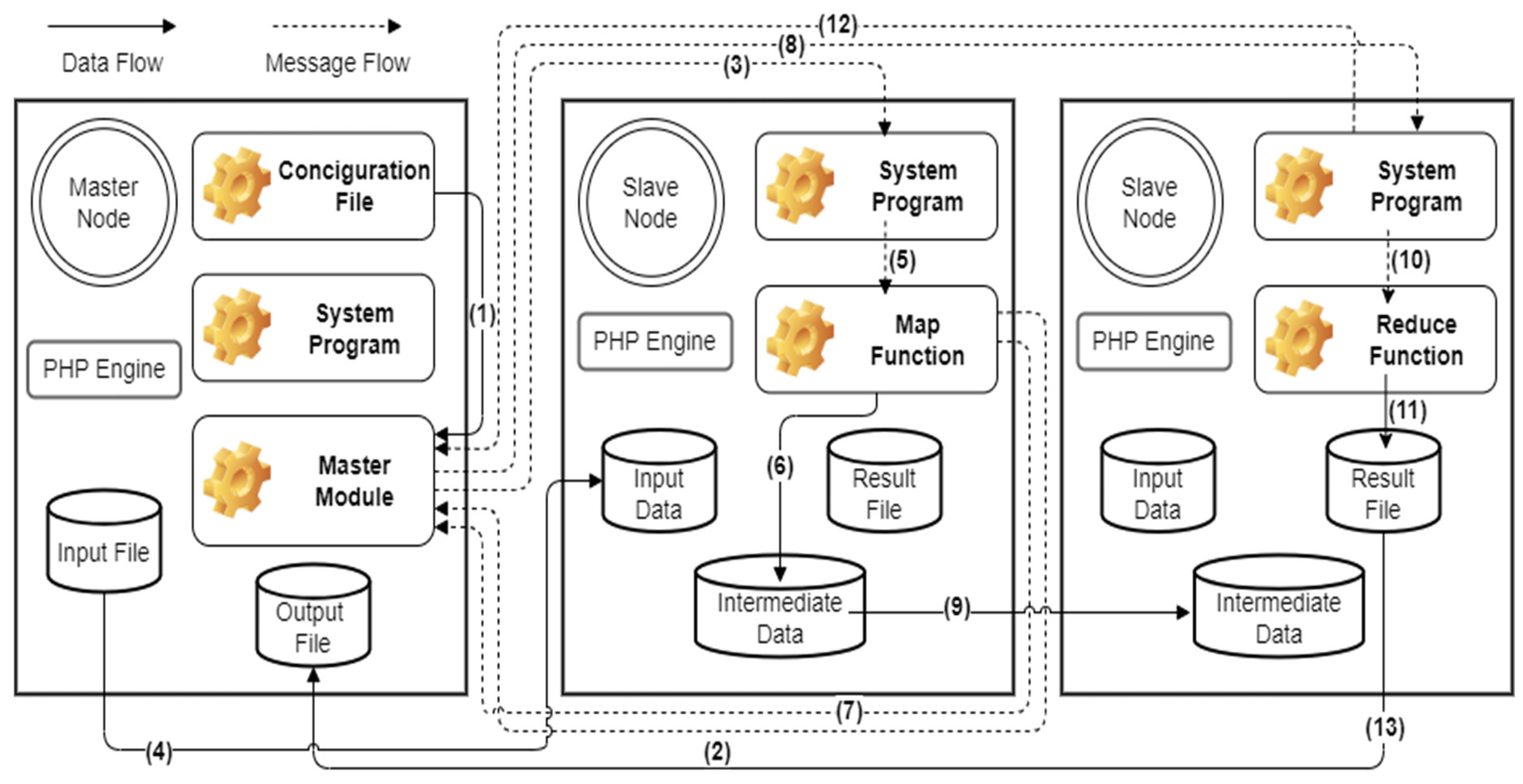
In this work, we systematically implemented a traditional MapReduce software architecture for small-scale cloud applications based on the recommendations in the literature [16,17,18,19]. Refer to Hadoop MapReduce framework for small-scale cloud architecture implementation of the DTAM in the PHP and C programming languages. In the small-scale cloud system used in this paper, a PHP program was used to realise the deployment task module, and a C program was used as the runtime system to transmit data and execute the cloud application tasks. The same system was installed on each slave node of the system, and the same environmental parameters were used. The implementation of the system is illustrated in Figure 4.

Before the system can execute a small-scale cloud application using the MapReduce framework, it must determine the relevant parameter settings and the content of the configuration file, which contains settings such as the location of the input-data source, the number of operating slave nodes, the maximum numbers of Map and Reduce tasks for each slave node, the application to be executed, the number of intermediate data and the key value of the intermediate-data partition to start the Reduce task. The master module on the master node reads the configuration file to determine the initial settings; it then communicates with the runtime system of each slave node to confirm that it can operate the application program normally, and at the same time, clears the input data for each slave node to ensure that there are no remaining unprocessed input data. The master module confirms the name of the input file and receives periodic information from each slave node that indicates the number of available Map tasks. The master module sends commands to its Map function, based on the IP location of each slave node, to perform the Map task. Since each slave node periodically returns the number of available Map tasks to the master module, the runtime system is used as a bridge to share the IP address of each node with the others. The Map tasks of each slave node use the IP address information of the runtime system to distribute the input file of the master module to the Map tasks of each slave node as input data. The Map task of each slave node processes the Map function application after receiving the above input data and generates intermediate data.

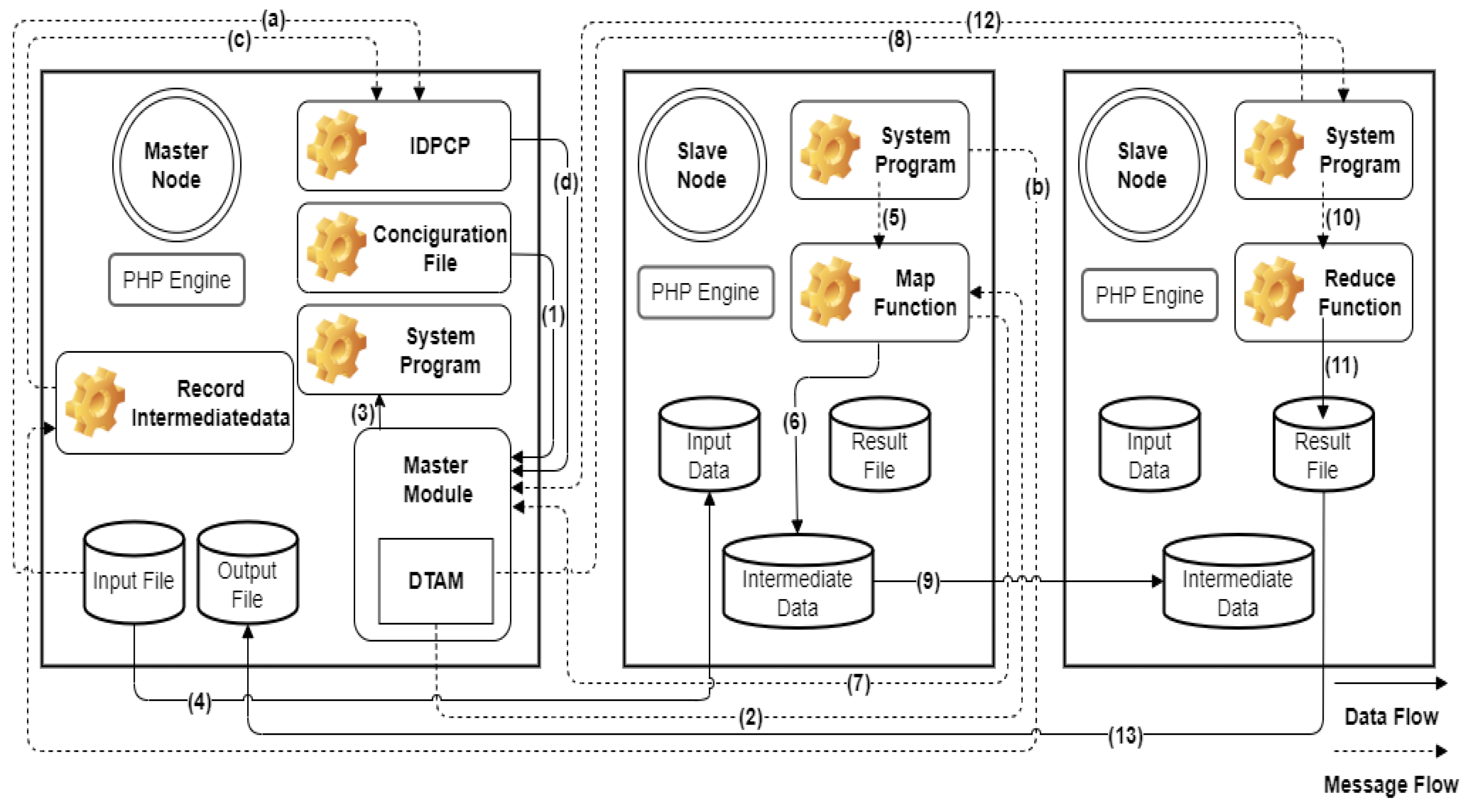
After the Map task is processed by each slave node, the master module is notified that the task is complete. The master module delivers to each specific slave node the available Reduce tasks for subsequent processing based on the K value of the intermediate data. The data are allocated to each slave node as the intermediate data of the Reduce task to process the Reduce function program. When the Reduce task has been processed by each slave node, a result file is generated and sent to the master module for integration. On completion of the Reduce task, the master module of the system notifies each slave node to return the result file, which is used to generate the output file. We implemented our algorithm, called DTAM with IDPCP, based on a traditional MapReduce architecture for small-scale cloud applications, as shown in Figure 5. The system uses the IDPCP algorithm to obtain the information on the input file and to integrate the maximum number of Map tasks for each slave node to calculate the wave number of future digestion input files. The intermediate-data information generated by the runtime system of each slave node for its Map task is recorded by the master module (‘Record Intermediate Data’ in Figure 5). The system implementation uses the size of the memory space as the intermediate-data accumulation record and predicts the volume of intermediate data to be generated by each slave node in the next cycle. The master module of the system uses this information to set upper limits on the numbers of Map and Reduce tasks for each slave node, in order to improve the processing efficiency and avoid the problem of performance degradation due to laggard nodes.

5. Results and Discussion

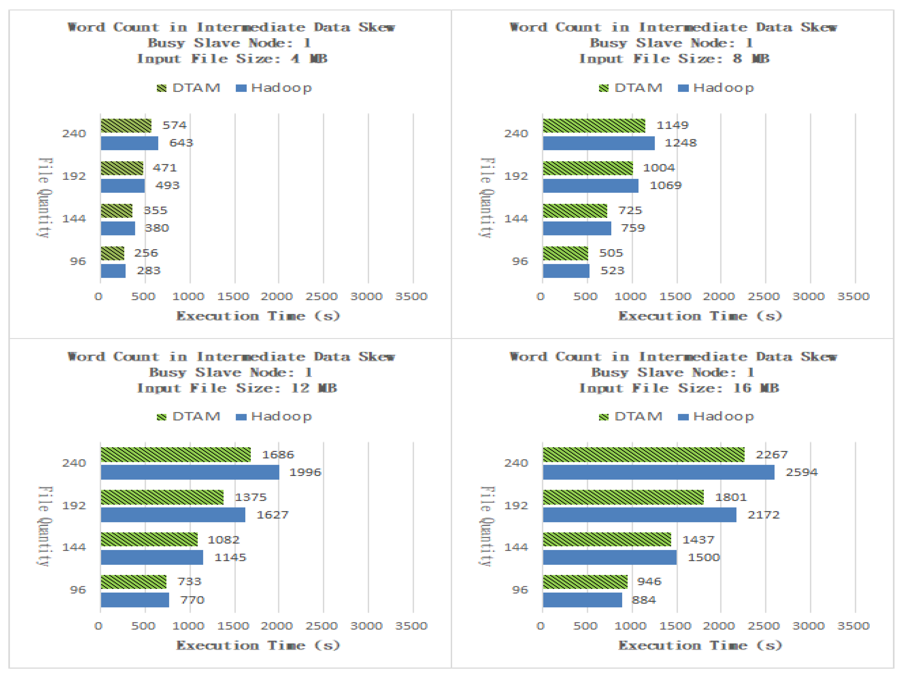
The experimental environment was based on nine identical computers with the following specifications: AMD Athlon II X6 1055T CPU, 4 GB memory, 500 GB hard disk and an Ethernet card. Because the CPU had six cores, we assign six to M_dn and R_dn, respectively, in all experiments. The cloud applications used in the experiment were Word Count, All Unique Combinations, Inverted Index, Radix Sort and Session Mean Value calculations. The input-data types of the Word Count and All Unique Combinations applications were from 001 to 008; the numbers of data files were 96, 144, 192 and 240; files of sizes 4, 8, 12 and 16 MB were used. We analysed the performance of our system and compared it with a simulation of a traditional Hadoop (Google Cloud platform) MapReduce framework. The Word Count application counts the number of all words in the input-data file. The Map task program generates intermediate data (such as Key = a, Value = 1) and records the information, and the Reduce task program processes all the intermediate-data files from each slave node. The summation calculation generates partial output files, and, finally, the master node unifies all of the partial output files from the slave nodes to obtain the final result file.

As shown in Figure 6, for files of size 4 MB, the performance of the DTAM on 96, 144, 192 and 240 files was better than that of Hadoop by 9.54%, 6.58%, 4.46% and 10.73%, respectively, and the overall average was better than that of the traditional method by 7.83%. As shown in Figure 6, for files of size 8 MB, the performance of the DTAM on 96, 144, 192 and 240 files was better than that of Hadoop by 3.34%, 4.48%, 6.08% and 7.93%, respectively, and the overall average was better than that of the traditional method by 5.48%. As shown in Figure 6, for files of size 12 MB, the performance of the DTAM on 96, 144, 192 and 240 files was better than that of Hadoop by 4.81%, 5.50%, 3.50% and 15.53%, respectively, and the overall average was better than that of the traditional method by 10.33%. As shown in Figure 6, for files of size 16 MB, the performance of the DTAM on 96, 144, 192 and 240 files was better than that of Hadoop by −7.01%, 4.20%, 17.08% and 12.61%, respectively, and the overall average was better than that of the traditional method by 6.72%. It can be seen from the experimental results that the proposed DTAM algorithm can reduce the problem of end time delay by dynamically adjusting the number of Map and Reduce tasks to disperse the workload of a busy slave node.

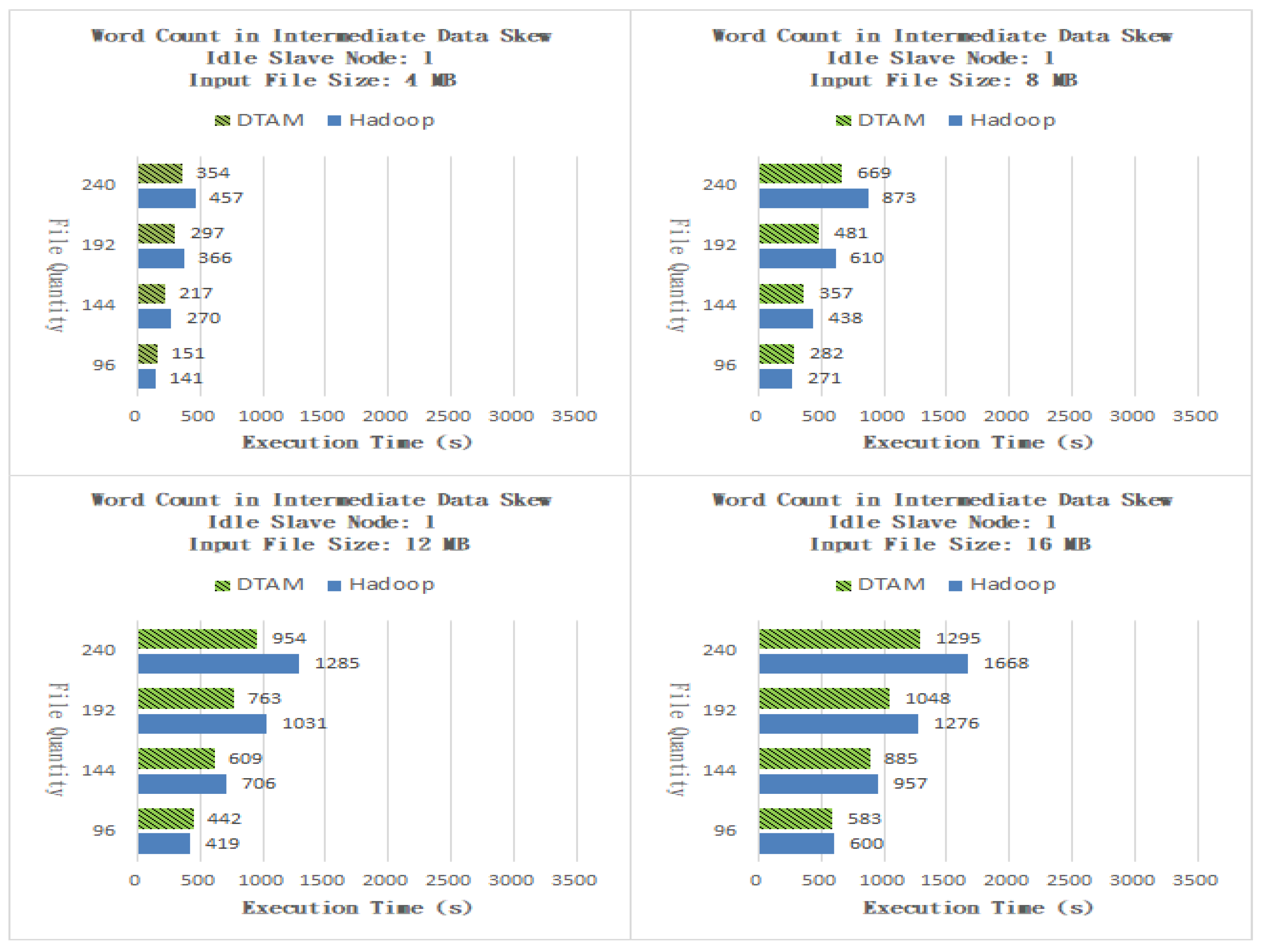
As shown in Figure 7, for files of size 4 MB, the performance of the DTAM on 96, 144, 192 and 240 files was better than that of Hadoop by −7.09%, 19.63%, 18.85% and 22.51%, respectively, and the overall average was better than that of the traditional method by 13.48%. As shown in Figure 7, for files of size 8 MB, the performance of the DTAM on 96, 144, 192 and 240 files was better than that of Hadoop by −4.06%, 18.49%, 21.15% and 23.37%, respectively, and the overall average was better than that of the traditional method by 14.74%. As shown in Figure 7, for files of size 12 MB, the performance of the DTAM on 96, 144, 192 and 240 files was better than that of Hadoop by −5.49%, 13.74%, 25.99% and 25.76%, respectively, and the overall average was better than that of the traditional method by 15.00%. As shown in Figure 7, for files of size of 16 MB, the performance of the DTAM on 96, 144, 192 and 240 files was better than that of Hadoop by 2.83%, 7.52%, 17.87% and 22.36%, respectively, and the overall average was better than that of the traditional method by 12.65%. From our results, it can be observed that the DTAM can increase the workload of idle slave nodes by dynamically adjusting the number of Map and Reduce program tasks to reduce the problem of end time delay.

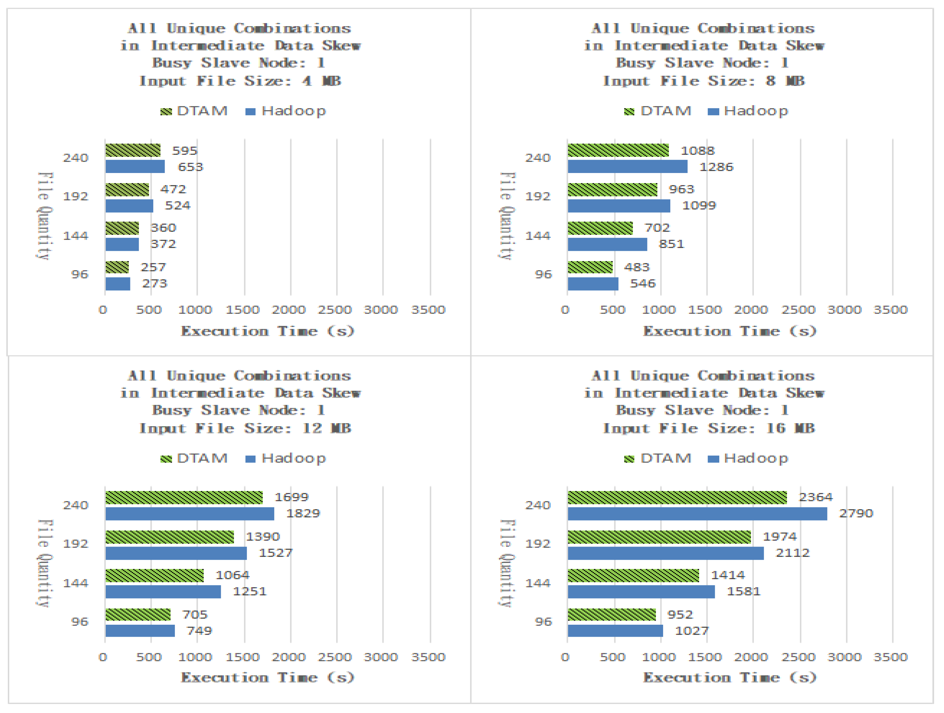
The All Unique Combinations application obtains a non-repetitive combination of all input-data numbers. The Map program generates intermediate data (such as Key = 1, Value = 1) and records this information. In the Reduce program, all non-repetitive values in all the intermediate-data files from the slave nodes are combined to generate all permutations and combinations and to create some output files. Finally, the master node unifies all the partial output files from the slave nodes and deletes identical entries to obtain the final result file.

As shown in Figure 8, for files of size 4 MB, the performance of the DTAM on 96, 144, 192 and 240 files was better than that of Hadoop by 5.86%, 3.23%, 9.92% and 8.88%, respectively, and the overall average was better than that of the traditional method by 6.97%. As shown in Figure 8, for files of size 8 MB, the performance of the DTAM on 96, 144, 192 and 240 files was better than that of Hadoop by 11.54%, 17.51%, 12.37% and 15.40%, respectively, and the overall average was better than that of the traditional method by 14.20%. As shown in Figure 8, for files of size 12 MB, the performance of the DTAM on 96, 144, 192 and 240 files was better than that of Hadoop by 5.87%, 14.95%, 8.97% and 7.11%, respectively, and the overall average was better than that of the traditional method by 9.23%. As shown in Figure 8, for files of size 16 MB, the performance of the DTAM on 96, 144, 192 and 240 files was better than that of Hadoop by 7.30%, 10.56%, 6.53% and 15.27%, respectively, and the overall average was better than that of the traditional method by 9.92%.

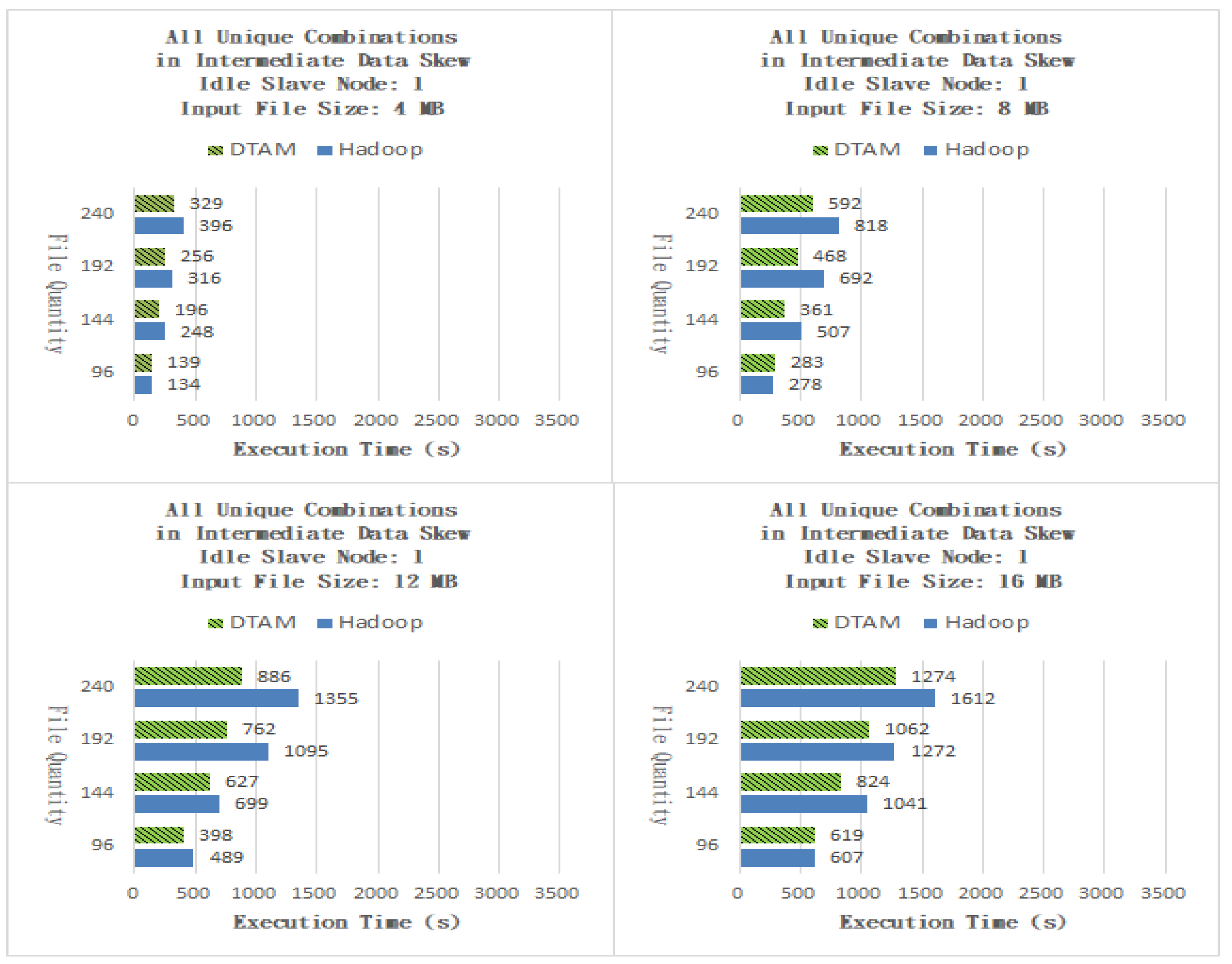
As shown in Figure 9, for files of size 4 MB, the performance of the DTAM on 96, 144, 192 and 240 files was better than that of Hadoop by −3.73%, 20.97%, 18.99% and 16.92%, respectively and the overall average was better than c the traditional method by 13.29%. As shown in Figure 9, for files of size 8 MB, the performance of the DTAM on 96, 144, 192 and 240 files was better than that of Hadoop by −1.80%, 28.80%, 32.37% and 27.63%, respectively and the overall average was better than that of the traditional method by 21.75%. As shown in Figure 9, for files of size 12 MB, the performance of the DTAM on 96, 144, 192 and 240 files was better than that of Hadoop by 18.61%, 10.30%, 30.41% and 34.61%, respectively and the overall average was better than that of the traditional method by 23.48%. As shown in Figure 9, for files of size 16 MB, the performance of the DTAM on 96, 144, 192 and 240 files was better than that of Hadoop by −1.98%, 20.85%, 16.51% and 20.97%, respectively and the overall average was better than that of the traditional method by 14.09%. It can be seen from the experimental results that the proposed DTAM algorithm can reduce the overall end time delay by dynamically adjusting the number of Map and Reduce program tasks to evenly distribute the workloads of the slave nodes.

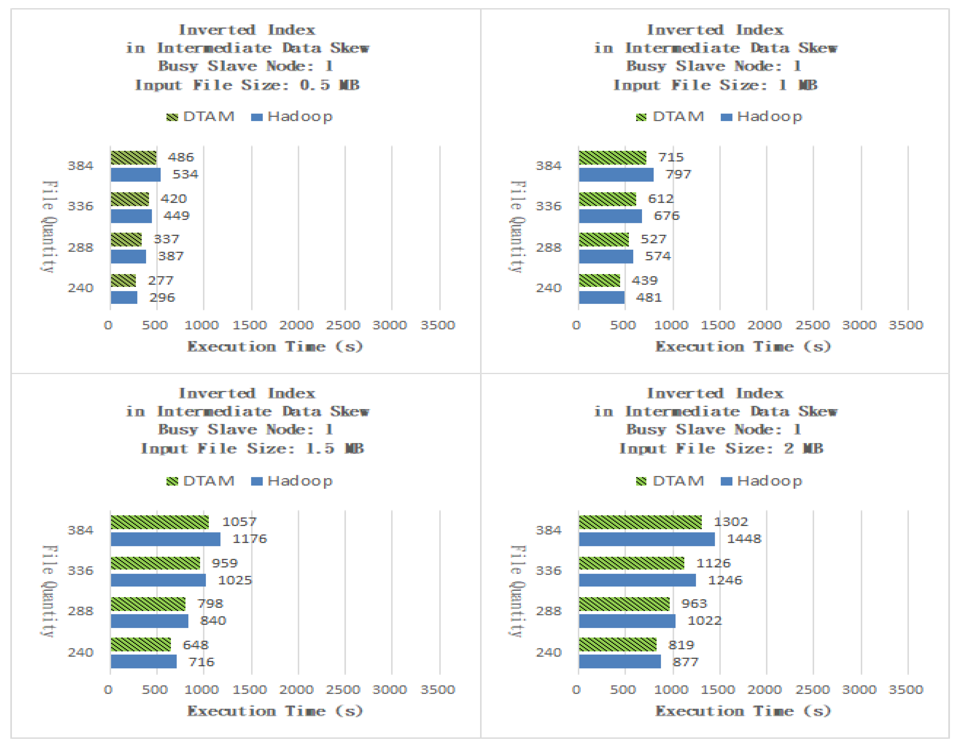
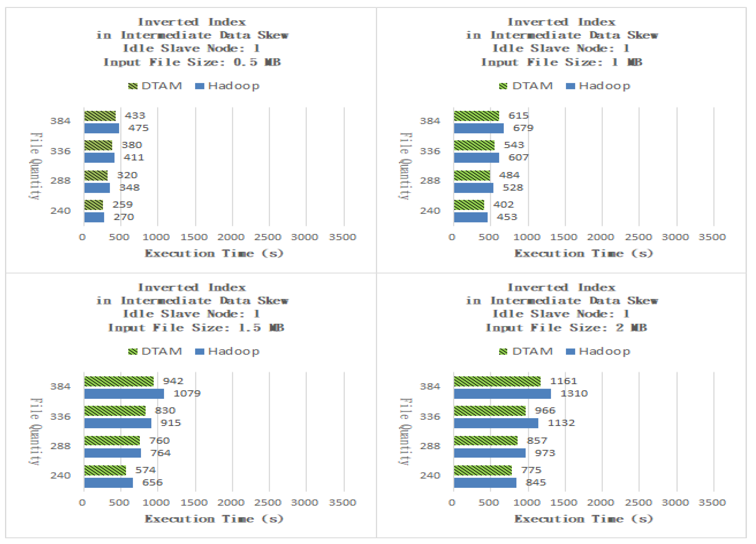
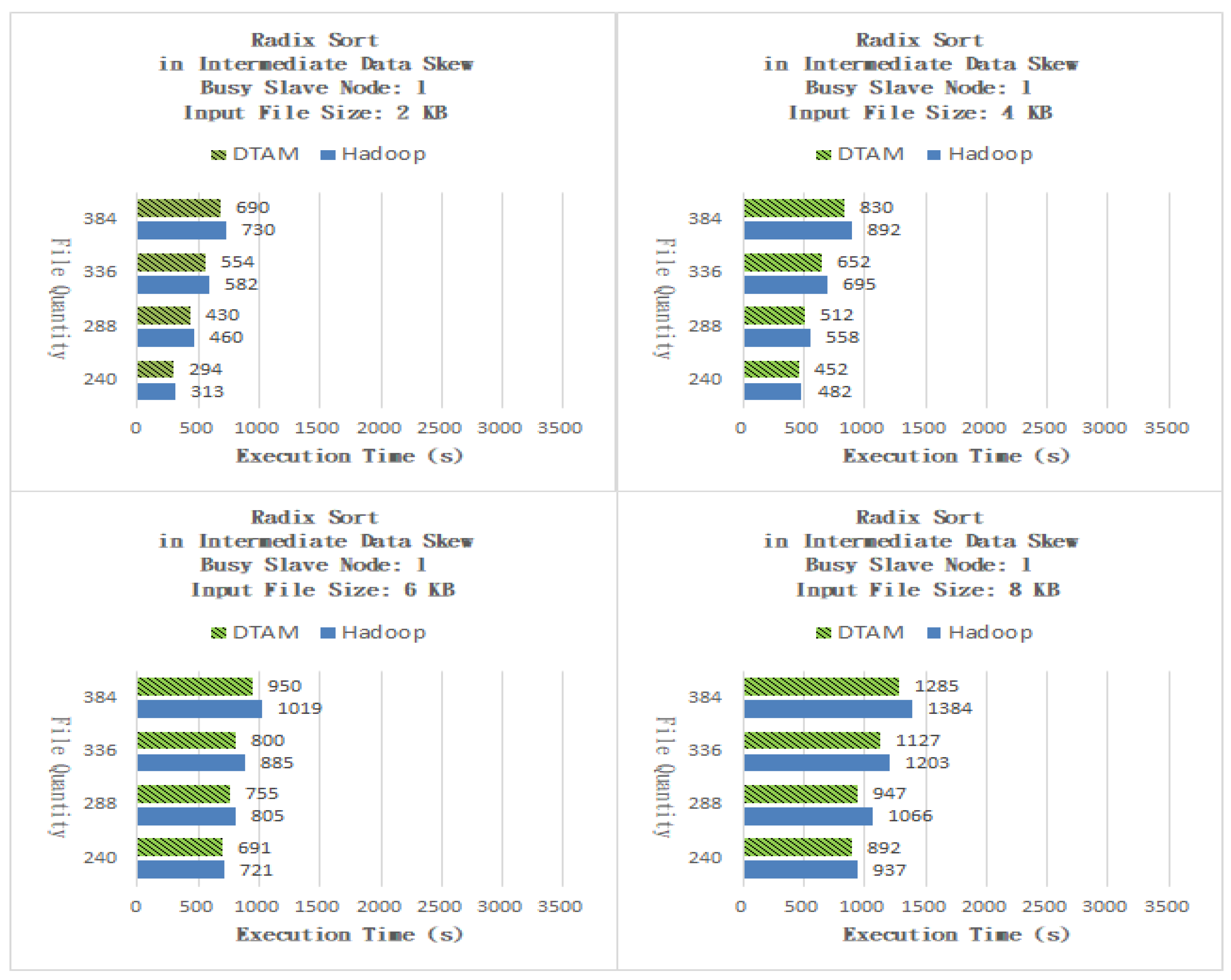
The Inverted Index application finds the locations of specific strings in the input file. In the Map task, the position information between the input-data words and the words is processed, and an intermediate-data file is generated. In the Reduce task program, the string position is recorded in a partial output file. Finally, the master node unifies all partial output files from the slave nodes to obtain the final search result file. As shown in Figure 10, the DTAM performed better than Hadoop by 8.70%, 9.17, 7.76% and 8.03% for files of sizes 0.5, 1, 1.5 and 2 MB, respectively. As shown in Figure 11, the DTAM performed better than Hadoop by 7.13%, 9.89, 8.75% and 11.56% for files of sizes 0.5, 1, 1.5 and 2 MB, respectively. From the experimental results, it can be seen that the proposed DTAM algorithm can mitigate the performance degradation for small-scale cloud applications caused by the phenomenon of laggards, by dynamically adjusting the number of Map and Reduce program tasks. The Radix Sort application sorts input-data content, which process the input-data content value segmentation in the Map program and generates intermediate-data files. When the Reduce program has completed the sorting job for each content value, the master node unifies all partial output files from the slave nodes to give the final result file.

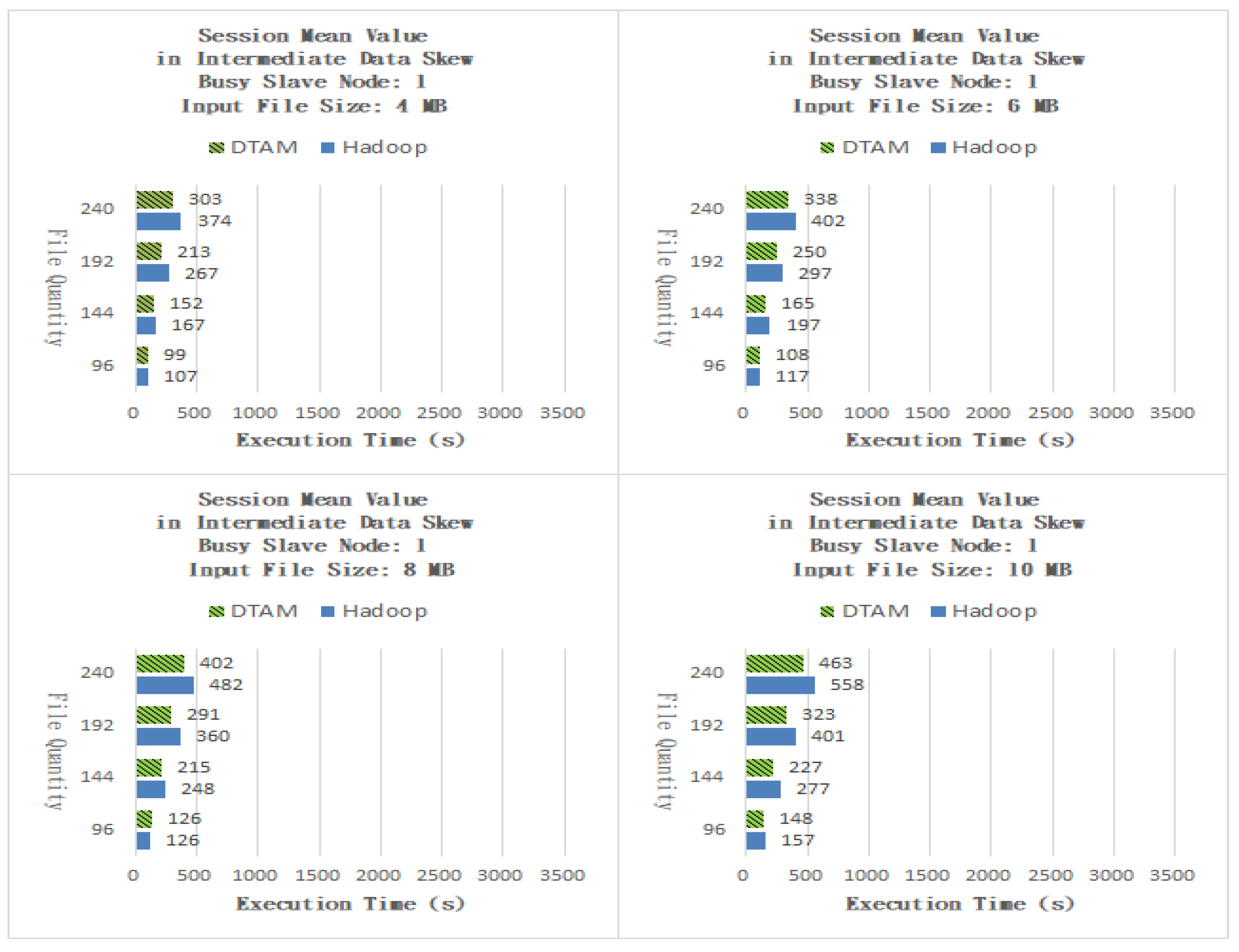
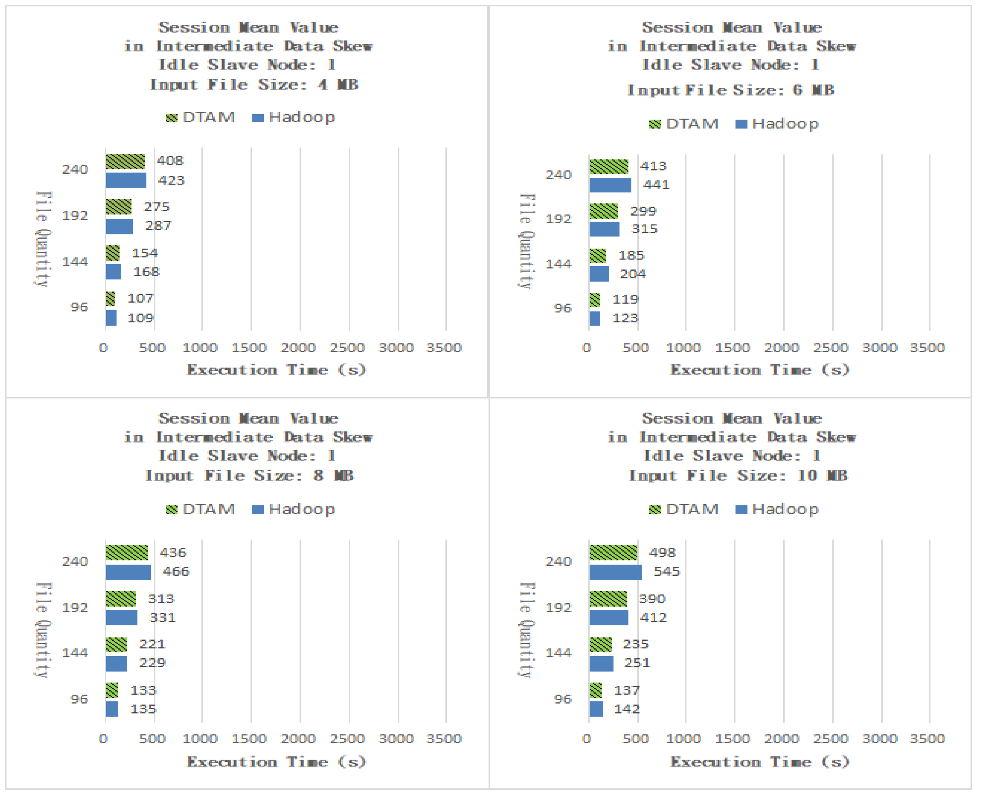
As shown in Figure 12, the DTAM performed better than Hadoop by 5.72%, 6.90%, 6.69% and 7.36% for files of sizes 0.5, 1, 1.5 and 2 MB, respectively. As shown in Figure 13, the DTAM performed better than Hadoop by 14.82%, 14.75%, 13.04% and 14.58% for files of sizes 0.5, 1, 1.5 and 2 MB, respectively. The experimental results indicate that our DTAM with IDPCP algorithm successfully adjusts the numbers of Map and Reduce tasks to mitigate the performance degradation of small-scale cloud applications caused by the phenomenon of laggards. The Session Mean Value application averages the input data. The Map task involves processing the sum of the same values and counting them, while in the Reduce task, the results of all the intermediate-data files from the slave nodes are directly summed up. Finally, the files are unified and averaged by the master node to give the final result. As shown in Figure 14, the DTAM performed better than Hadoop by 13.92%, 13.92%, 12.27% and 15.06% for files of sizes 0.5, 1, 1.5 and 2 MB, respectively. As shown in Figure 15, the DTAM performed better than Hadoop by 4.47%, 6.00%, 4.21% and 5.96% for files of sizes 0.5, 1, 1.5 and 2 MB, respectively. Our experimental results show that the DTAM with IDPCP algorithm can give an improvement and can avoid exceeding the maximum number of tasks set for each slave node. It is limited by the phenomenon of laggard nodes, which degrades the performance of small-scale cloud applications.

6. Conclusions

In view of the problem of intermediate-data skew affecting the processing efficiency of the MapReduce cloud architecture, we propose an algorithm called DTAM with IDPCP, which predicts the number of intermediate data that is expected to be produced by each slave node in the future by dividing the input data into a number of processing wavenumber periods. The algorithm dynamically adjusts the number of Map and Reduce tasks allocated to the slave nodes and avoids exceeding the maximum number of tasks set by the manager of each slave node. The workload is evenly distributed over the slave nodes to reduce the problem of end time delay. The DTAM algorithm proposed in this paper was compared with a simulated Hadoop (Google Cloud platform) system in a performance analysis and was shown to achieve an increase in processing efficiency of at least 5%. The algorithm proposed in this paper dynamically adjusts the number of Map and Reduce tasks according to the size of the intermediate-data and input-data files generated by each slave node. In the future, data type analysis should be performed on the input data and intermediate data to completely solve the problem of intermediate-data skew in the MapReduce cloud architecture.

References

- Kalia, K.; Gupta, N. Analysis of Hadoop MapReduce Scheduling in Heterogeneous Environment. Elsevier Ain Shams Eng. J. 2021, 12, 1101–1110. [Google Scholar] [CrossRef]
- Dong, J.; Goebel, R.; Hu, J.; Lin, G.; Su, B. Minimizing Total Job Completion Time in MapReduce Scheduling. Elsevier Comput. Ind. Eng. J. 2021, 158, 107387–107396. [Google Scholar] [CrossRef]
- Singh, G.; Sharma, A.; Jeyaraj, R.; Paul, A. Handling Non-Local Executions to Improve MapReduce Performance Using Ant Colony Optimization. IEEE Access J. 2021, 9, 96176–96188. [Google Scholar] [CrossRef]
- Kadkhodaei, H.; Moghadam, A.; Dehghan, M. Big Data Classification using Heterogeneous Ensemble Classifiers in Apache Spark based on MapReduce Paradigm. Elsevier Expert Syst. Appl. J. 2021, 183, 115369–115386. [Google Scholar] [CrossRef]
- Shieh, C.; Huang, S.; Sun, L.; Tsai, M.; Chilamkurti, N. A Topology-based Scaling Mechanism for Apache Storm. Wiley Int. J. Netw. Manag. 2016, 27, e1933. [Google Scholar] [CrossRef]
- Huang, T.; Shieh, C.; Chilamkurti, N.; Tsai, M.; Rho, S. Architecture for Speeding up Program Execution with Cloud Technology. Springer J. Supercomput. 2016, 72, 3601–3618. [Google Scholar] [CrossRef]
- Tang, Z.; Lv, W.; Li, K.; Li, K. An Intermediate Data Partition Algorithm for Skew Mitigation in Spark Computing Environment. IEEE Trans. Cloud Comput. J. 2021, 9, 461–474. [Google Scholar] [CrossRef]
- Liu, G.; Zhu, X.; Wang, J.; Guo, D.; Bao, W.; Guo, H. SP-Partitioner: A Novel Partition Method to Handle Intermediate Data Skew in Spark Streaming. Elsevier Future Gener. Comput. Syst. J. 2018, 89, 1054–1063. [Google Scholar] [CrossRef]
- Li, C.; Zhang, Y.; Luo, Y. Intermediate Data Placement and Cache Replacement Strategy under Spark Platform. Elsevier J. Parallel Distrib. Comput. 2022, 163, 114–135. [Google Scholar] [CrossRef]
- Irandoost, M.; Rahmani, A.; Setayeshi, S. A Novel Algorithm for Handling Reducer Side Data Skew in MapReduce based on a Learning Automata Game. Elsevier Inf. Sci. J. 2019, 501, 662–679. [Google Scholar] [CrossRef]
- Chen, Q.; Yao, J.; Xiao, Z. LIBRA: Lightweight Data Skew Mitigation inMapReduce. IEEE Trans. Parallel Distrib. Syst. J. 2015, 26, 2520–2533. [Google Scholar] [CrossRef]
- Tang, Z.; Ma, W.; Li, K.; Li, K. A Data Skew Oriented Reduce Placement Algorithm Based on Sampling. IEEE Trans. Cloud Comput. J. 2016, 8, 1149–1161. [Google Scholar] [CrossRef] [Green Version]
- Fan, Y.; Wu, W.; Xu, Y.; Chen, H. Improving MapReduce Performance by Balancing Skewed Loads. J. China Commun. 2014, 11, 85–108. [Google Scholar] [CrossRef]
- Guo, Y.; Rao, J.; Jiang, C.; Zhou, X. Moving Hadoop into the Cloud with Flexible Slot Management and Speculative Execution. IEEE Trans. Parallel Distrib. Syst. J. 2017, 28, 798–812. [Google Scholar] [CrossRef]
- Vinutha, D.; Raju, G. Node Performance Load Balancing Algorithm for Hadoop Cluster. In Proceedings of the IEEE International Conference on Intelligent Sustainable Systems, Palladam, India, 21–22 February 2019; pp. 468–473. [Google Scholar]
- Dean, J.; Ghemawat, S. MapReduce: Simplified Data Processing on Large Clusters. Commun. ACM J. 2008, 51, 107–113. [Google Scholar] [CrossRef]
- Krishnan, S.; Baru, C.; Crosby, C. Evaluation of MapReduce for Gridding LIDAR Data. In Proceedings of the IEEE International Conference on Cloud Computing Technology and Science, Indianapolis, IN, USA, 30 November–3 December 2010; pp. 33–40. [Google Scholar]
- Huang, T.; Chu, K.; Lee, W.; Ho, Y. Adaptive Combiner for MapReduce on cloud computing. Clust. Comput. J. 2014, 17, 1231–1252. [Google Scholar] [CrossRef]
- Shih, J.; Liao, C.; Chang, R. Simplifying MapReduce Data Processing. In Proceedings of the IEEE International Conference on Utility and Cloud Computing, Melbourne, Australia, 5–8 December 2011; pp. 366–370. [Google Scholar]
Figure 1.
MapReduce parallel computing framework.
Figure 2.
A traditional small-scale cloud system.
Figure 3.
Overview of the dynamic task allocation mechanism.
Figure 4.
Flowchart showing the implementation of a traditional small-scale cloud system.
Figure 5.
Flowchart for the implementation of a small-scale cloud system with DTAM.
Figure 6.
Word Count with one busy slave node.
Figure 7.
Word Count with one idle slave node.
Figure 8.
All Unique Combinations with one busy slave node.
Figure 9.
All Unique Combinations with one idle slave node.
Figure 10.
Inverted Index with one busy slave node.
Figure 11.
Inverted Index with one idle slave node.
Figure 12.
Radix Sort with one busy slave node.
Figure 13.
Radix Sort with one idle slave node.
Figure 14.
Session Mean Value with one busy slave node.
Figure 15.
Session Mean Value with one idle slave node.
Publisher’s Note: MDPI stays neutral with regard to jurisdictional claims in published maps and institutional affiliations. |
© 2022 by the authors. Licensee MDPI, Basel, Switzerland. This article is an open access article distributed under the terms and conditions of the Creative Commons Attribution (CC BY) license (https://creativecommons.org/licenses/by/4.0/).
Share and Cite
MDPI and ACS Style
Huang, T.-C.; Huang, G.-H.; Tsai, M.-F. Improving the Performance of MapReduce for Small-Scale Cloud Processes Using a Dynamic Task Adjustment Mechanism. Mathematics 2022, 10, 1736. https://doi.org/10.3390/math10101736
AMA Style
Huang T-C, Huang G-H, Tsai M-F. Improving the Performance of MapReduce for Small-Scale Cloud Processes Using a Dynamic Task Adjustment Mechanism. Mathematics. 2022; 10(10):1736. https://doi.org/10.3390/math10101736
Chicago/Turabian StyleHuang, Tzu-Chi, Guo-Hao Huang, and Ming-Fong Tsai. 2022. "Improving the Performance of MapReduce for Small-Scale Cloud Processes Using a Dynamic Task Adjustment Mechanism" Mathematics 10, no. 10: 1736. https://doi.org/10.3390/math10101736
Note that from the first issue of 2016, this journal uses article numbers instead of page numbers. See further details here.