Article

A Non-Integer High-Order Sliding Mode Control of Induction Motor with Machine Learning-Based Speed Observer

1
School of Electrical and Electronics Engineering, Chung-Ang University, Dongjak-gu, Seoul 06974, Republic of Korea
2
Department of Electrical Engineering, University of Engineering and Technology Peshawar, Bannu Campus, Bannu 28100, Pakistan
3
Electrical Engineering, CECOS University of IT & Emerging Sciences, Peshawar 25000, Pakistan
4
Department of Electrical Engineering, Sukkur IBA University, Sukkur 65200, Pakistan
5
Department of Astronautical, Electrical and Energy Engineering, University of Rome “La Sapienza”, 00184 Rome, Italy
6
Department of Intelligent Energy and Industry, Chung-Ang University, Dongjak-gu, Seoul 06974, Republic of Korea
*
Author to whom correspondence should be addressed.
These authors contributed equally to this work.
Machines 2023, 11(6), 584; https://doi.org/10.3390/machines11060584
Submission received: 14 April 2023 / Revised: 9 May 2023 / Accepted: 16 May 2023 / Published: 24 May 2023

Abstract

:
The induction motor (IM) drives are prone to various uncertainties, disturbances, and non-linear dynamics. A high-performance control system is essential in the outer loop to guarantee the accurate convergence of speed and torque to the required value. Super-twisting sliding mode control (ST-SMC) and fractional-order calculus have been widely used to enhance the sliding mode control (SMC) performance for IM drives. This paper combines the ST-SMC and fractional-order calculus attributes to propose a novel super-twisting fractional-order sliding mode control (ST-FOSMC) for the outer loop speed control of the model predictive torque control (MPTC)-based IM drive system. The MPTC of the IM drive requires some additional sensors for speed control. This paper also presents a novel machine learning-based Gaussian Process Regression (GPR) framework to estimate the speed of IM. The GPR model is trained using the voltage and current dataset obtained from the simulation of a three-phase MPTC based IM drive system. The performance of the GPR-based ST-FOSMC MPTC drive system is evaluated using various test cases, namely (a) electric fault incorporation, (b) parameter perturbation, and (c) load torque variations in Matlab/Simulink environment. The stability of ST-FOSMC is validated using a fractional-order Lyapunov function. The proposed control and estimation strategy provides effective and improved performance with minimal error compared to the conventional proportional integral (PI) and SMC strategies.

1. Introduction

Nowadays, fractional calculus is widely used in engineering and scientific applications. Most of the scientists and researchers use fractional calculus to model their plants/systems to incorporate system dynamics, complex processes, and phenomena. For the last few decades, it has been widely used to improve the performance of controllers. The proportional integral derivative (PID) controller is modified as a Fractional PID controller, denoted as PI λ D [1,2,3], where the improved performance has drawn researchers to incorporate the advantage of fractional calculus in control paradigms. Other applications of fractional calculus can be found in adaptive fractional-order control schemes [4,5] and fractional-order sliding mode control (FOSMC) paradigms [6,7,8]. FOSMC schemes have shown their advantages against integer order sliding mode control (IOSMC) schemes and are evident in the literature. The author of [9] proposes a fractional-order fuzzy sliding mode control to remove uncertainty in active power filters with smaller total harmonic distortion (THD). The author of [10] introduces FOSMC for a space-tethered system to eliminate chattering and faster deployment time without overshoot. This paper aims to investigate the performance of FOSMC schemes in the IM drive system. Robust control approaches are widely used due to their robustness against the external turbulence and uncertainties in the non-linear systems. One of the control techniques is the direct torque control (DTC) method used in high-performance motors, which has the benefits of a wide range of speed control, high dynamic performance, and full load torque at zero speed. The DTC method uses two loops to control the speed and torque of IM, known as the inner loop and outer loop. The inner loop uses a controller to generate reference torque from the speed error. The outer loop generally uses hysteresis control or Space Vector Modulation to generate switching signals. These techniques are subjected to problems such as high harmonics in the torque and speed, unwanted noises, and extra losses due to un-optimized switching signals. Model predictive torque control (MPTC), a widely used technique used to overcome the shortcomings of the hysteresis-based DTC technique in the inner loop, is used in this paper. The MPTC drive system performance is further enhanced by the applications of a robust non-linear control system design. SMC is one of the widely used techniques in IM drives. I. Sami et al. proposed sliding mode control (SMC) in [11] for the MPTC-based IM drive. The SMC provides improved performance in terms of faults perturbations, speed tracking, less overshoot, and load torque variations. Numerous enhancement techniques have been proposed to improve the performance of the SMC in terms of chattering effect and disturbance rejection capabilities such as sliding surface designs, high-order SMC, modifications in reaching law, and combining the intelligent techniques with conventional SMC. These enhancement methods are summarized in Figure 1.
Fractional-order SMC (FOSMC) applications are increasing for electric drives applications. Unlike integer-order controllers, FOSMC uses integration and derivations of fractional order. Fractional-order surface involves generalization of integer-order surfaces, where the integer-order surfaces are modified using fractional-order integration and derivation. The author in [12] proposes a neuro fuzzy-based fractional-order control scheme for perturbed systems. Similarly, the authors of [13] use FOSMC with terminal SMC for doubly fed induction generator based wind energy system. A smooth and chattering free response has been reported in the proposed FOSMC technique. In this paper, conventional SMC is enhanced by combining fractional-order calculus-based sliding surface design and super-twisting (ST) SMC, hereafter called super-twisting fractional-order sliding mode control (ST-FOSMC). Rotor speed, stator currents, and electromagnetic currents are required for ST-FOSMC-based MPTC measurements using different sensors. When no sensors are used to measure the speed in IM drives, such systems are known as “sensorless systems” [14]. The terminal variables, namely current and voltage, are measured using sensors that are processed to estimate the speed, torque, and flux. The signals obtained through the sensors possess noise. Thus, sensors will insert a DC offset value to the measured values that can cause a saturation effect in the speed estimators. Sensorless control techniques are commonly used in the control applications of IM due to the high cost of the speed sensors and their difficulty in installation for industrial applications. The sensorless control methods minimize the noise level and the maintenance cost of the system [14]. The various techniques that are prominent in the literature are full-order observers, open-loop estimators, reduced-order observers, the Kalman filter, an adaptive reference model, and neural networks [15]. Various speed estimation techniques were developed in the literature. The recently used sliding mode observer (SMO)-based drive systems hold some smart topographies, for example: (a) its robustness to the variations in parameters and uncertainties in a model that are not sensitive to the variations in external load, (b) fast-active response, and steady control system; (c) its ability to withhold various non-linear systems, and, (d) its simple software/hardware operation. This strategy was employed to estimate and control the state of the system, as presented in [16]. The SMC scheme used a state-dependent control law switched at high frequency. The authors of [17] present a rotor speed and resistance observer design. The author of [18] uses a higher-order SMO, aiming to eliminate some inconveniences of the first-order SM, while still maintaining its main features. An SMO was also developed by [19] to estimate the speed of IM, but SMO is subjected to integration errors and severe chattering. The error in the rotor speed existed due to the chattering effect, which is still a big problem. An adaptive speed and resistance observer based on backstepping rules has been presented by Rasmussen et al. [20] using a superimposed square wave on the magnetizing current. The author of [21] proposed the use of a Kalman filter leading to unavoidable linearization error, thus compromising the estimation accuracy. Much-Simplified IM models had been used for speed estimation to overcome such limitations. An extended Kalman filter (EKF) was used by [22] to estimate the speed of IM. Furthermore, the accuracy was further improved by using an adaptive EKF in [23]. The EKF operation is based on the linearization of the non-linear IM system. The accuracy of speed observation is compromised by using linearization of a non-linear dynamic system. The authors of [24] proposed the unscented Kalman filter (UKF) to estimate the speed of IM. The UKF estimated the speed of IM without linearizing the system. The UKF estimates the speed using a set of sample points called sigma points. The UKF eliminates the linearization error at the cost of high computational complexity. Other Kalman filter-based online speed estimation techniques included switching EKF [25], braided EKF [26], and bi-input EKF [27]. The speed of the IM estimates was accomplished using rotor slot harmonics [28]. However, the rotor slot harmonics extraction confronts some vital difficulties in the very high or low-speed operating regions. The author of [29] estimated the speed of IM as a function of current and voltage using feed-forward neural network (NN) for efficient prediction based on previous observations [30,31,32]. A speed estimation methodology based on a radial basis function (RBF) artificial neural network was presented in [33]. Keeping in view the above considerations, a machine learning-based Gaussian process regression (GPR) framework with which to estimate the motor speed is proposed in this paper. The effectiveness of GPR-based estimated speed and the ST-FOSMC MPTC scheme shown in Figure 2 is validated using Matlab/Simulink. Its performance is also compared with conventional PI and SMC. The ST-FOSMC provided good speed convergence and robustness with minimum chattering. With the inclusion of the ST algorithm, the number of gains to be tuned increases, which makes the process complex. Hence, the gains are tuned using the optimization toolbox in Matlab/Simulink to achieve the required performances. Moreover, unlike the work presented in [12,34] using neuro-fuzzy sliding mode and fractional-order systems, this paper emphasizes chattering elimination using fractional calculus and uses the statistical method to estimate speed. More specifically, the contributions of our work are:
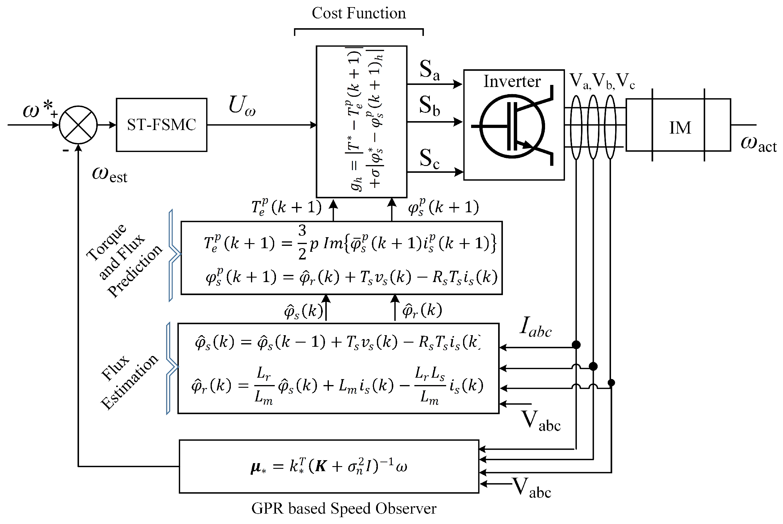
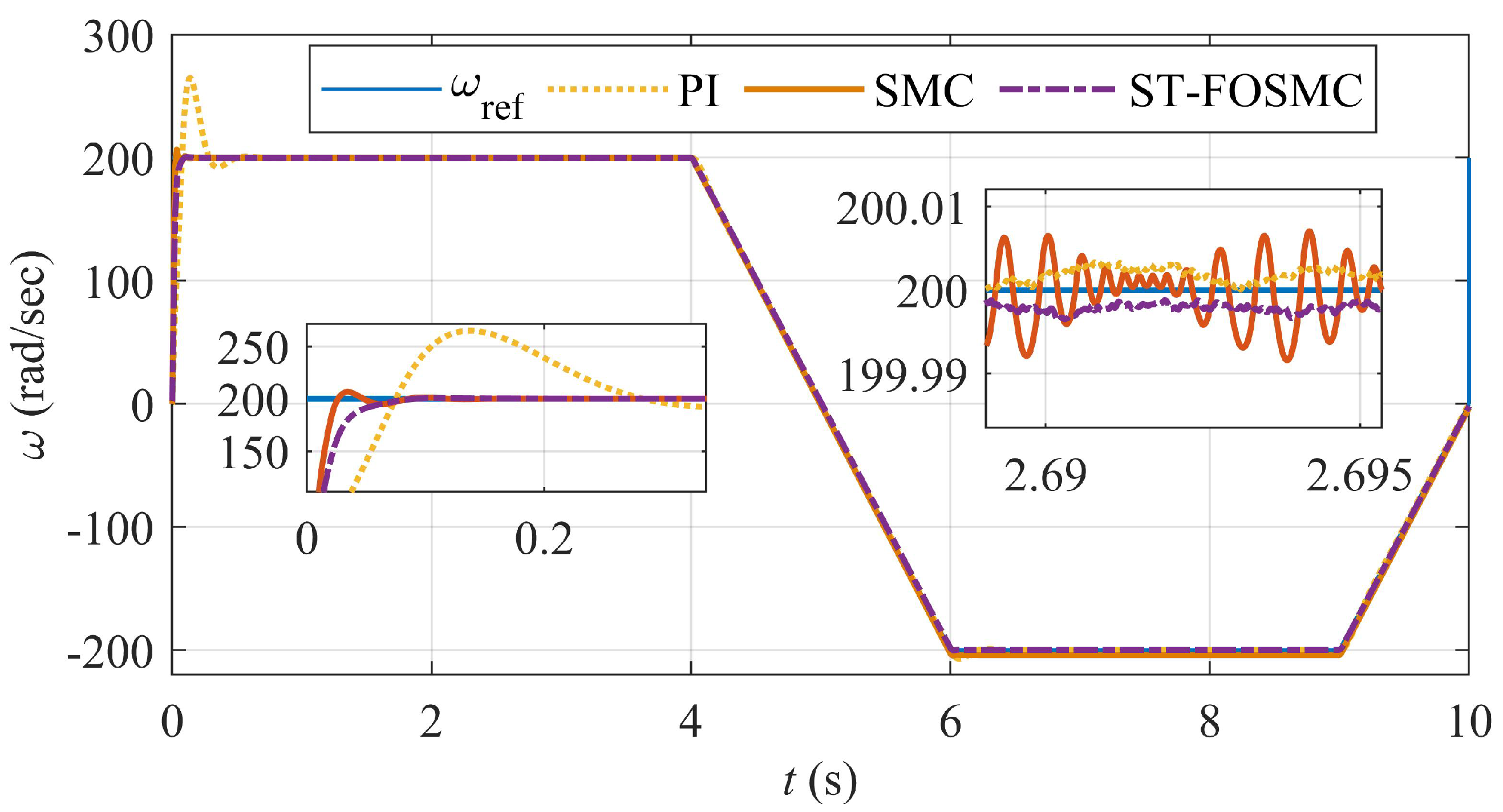
  • We propose a new control scheme called ST-FOSMC that combines Fractional-Order Sliding Mode Control (FOSMC) and Super-Twisting (ST) algorithms. We use FOSMC to shape the error dynamics of the system for robustness against disturbances and uncertainties, while ST is used for fast convergence and high-performance tracking. We evaluate the stability of the proposed control system by analyzing the ST and FOSMC error dynamics, which represent the difference between desired and actual states of the system and the deviation from the sliding surface defined by FOSMC, respectively. By studying the behavior of both error dynamics, we ensure the stability of the closed-loop system. Our proposed ST-FOSMC scheme achieves a robust and high-performance control with guaranteed stability.
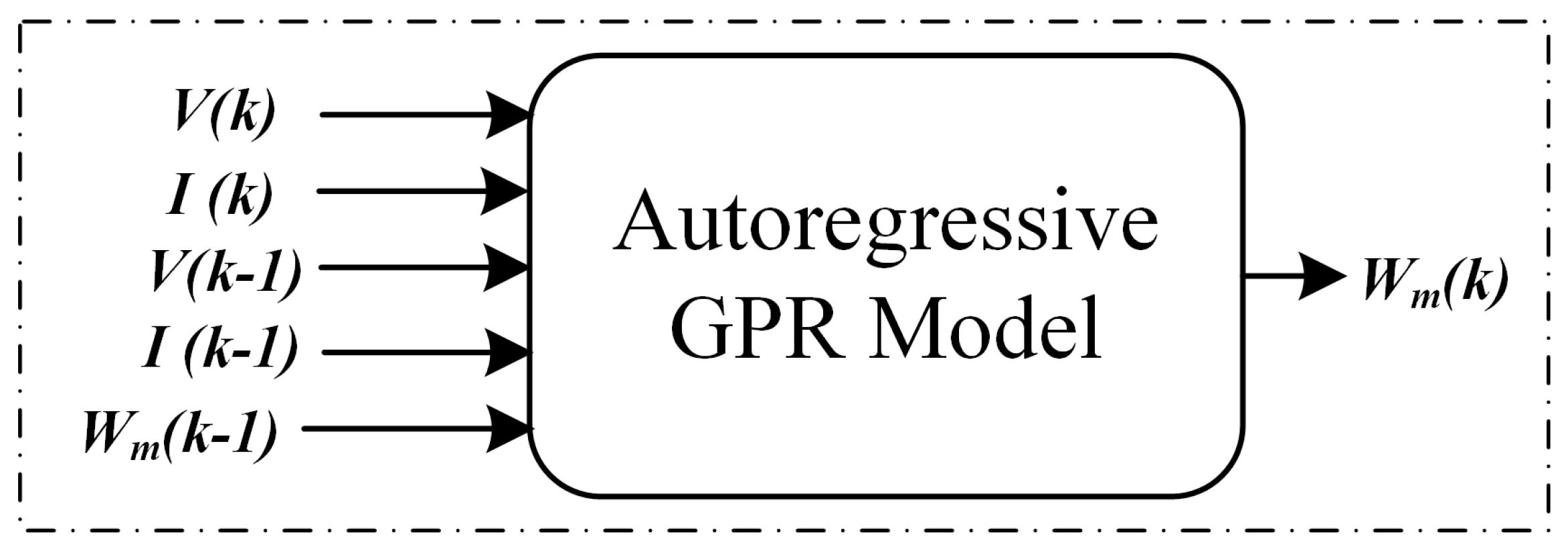
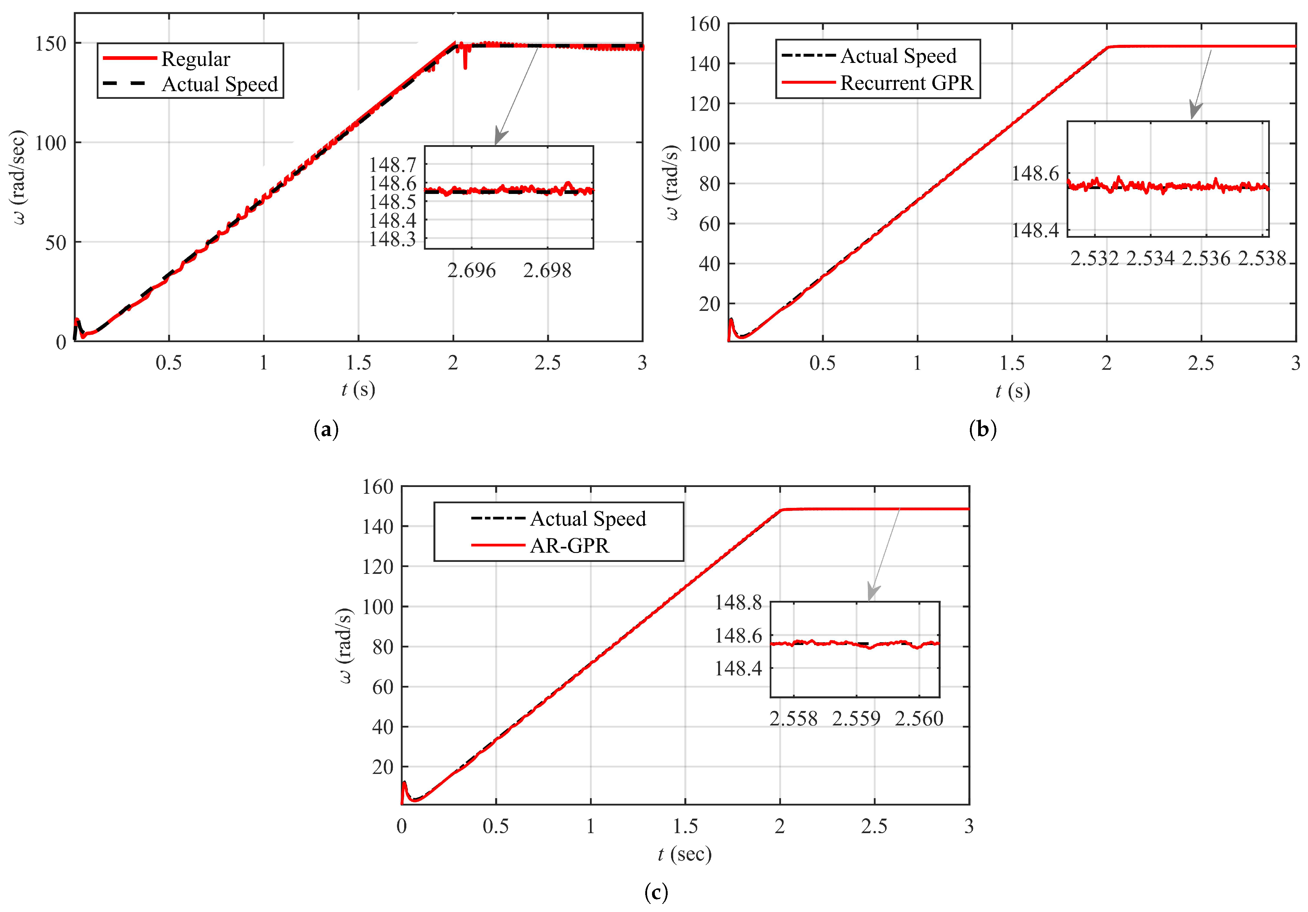
  • Our work proposes a machine learning-based method, specifically GPR, to estimate the speed of an Induction Motor (IM). The proposed GPR utilize an autoregressive (AR) GPR method that incorporates the estimated speed, voltage, and current from the previous discrete time to improve the accuracy of speed estimation. GPR is a non-parametric probabilistic model that is capable of accurately estimating the speed of an IM. By using an autoregressive approach, we are able to leverage the previously estimated speed, voltage, and current values to further enhance the accuracy of the estimation. Our proposed GPR-based method offers a reliable and accurate means of speed estimation for IM, which is crucial for effective motor control. This method has the potential to improve the efficiency and performance of IM control systems, especially in applications where precise speed control is critical.
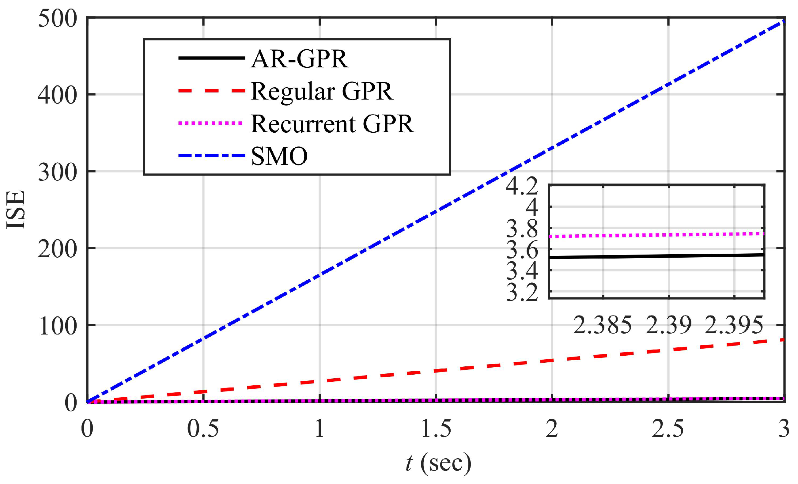
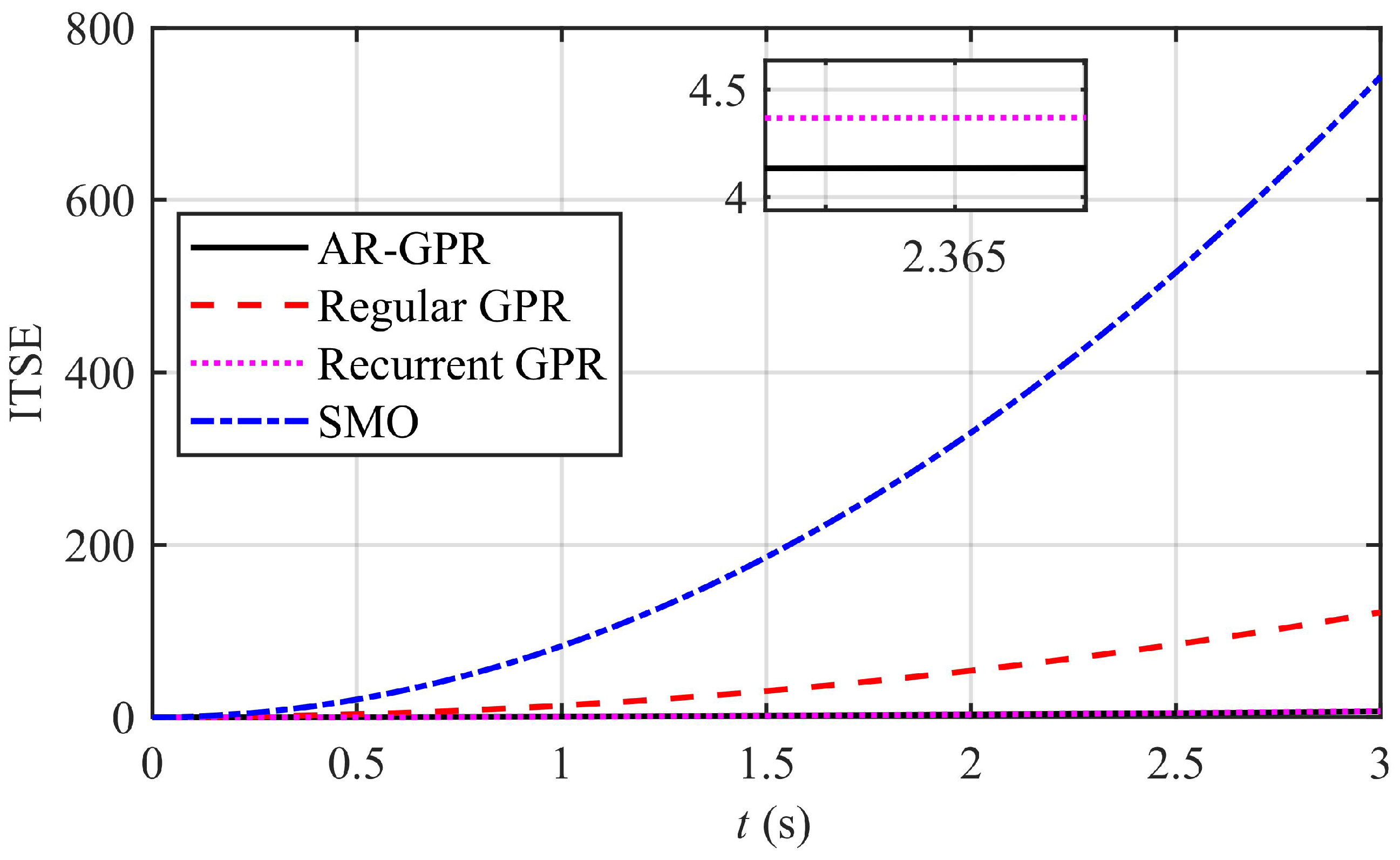
  • Comparative analysis of the GPR framework with a state-of-the-art SMO is also performed. Both the observers are evaluated through different performance indices, including integral square error, integral time square error, and root mean square error. The superiority of the proposed GPR framework-based ST-FOSMC scheme are also verified using various performance indices, stability, and robustness test, and comparisons with existing control methods.
The paper is structured as follows: Section 2 provides an overview of the basics of fractional calculus. The mathematical model of IM in a synchronously revolving reference frame is explained in Section 3, while Section 4 covers the modeling of MPTC. The proposed ST-FOSMC control paradigm is mathematically formulated in Section 5. The GPR framework is used to statistically model the IM, and this is detailed in Section 6. The Lyapunov stability of the proposed GPR speed observer in presented in Section 6.1. Section 7 presents the results of the simulation conducted in Matlab/Simulink to evaluate the performance of the proposed approach. Finally, Section 8 provides a conclusion to the paper.

2. Basic Definitions for Fractional Calculus

A fractional-order operator is a generalization of the traditional integer-order operators, such as differentiation and integration. It extends the concept of differentiation and integration to non-integer orders, allowing for more flexible and accurate modeling of complex systems. Fractional-order operators are defined using fractional calculus, which deals with derivatives and integrals of non-integer orders. Fractional calculus is a field of mathematics that has gained significant attention in recent years due to its wide-ranging applications in various fields, including physics, engineering, and finance. The fractional order operator is a powerful tool for modeling complex systems with memory and long-range dependencies. It can capture the inherent non-linearities and time-varying dynamics of real-world systems, which are often difficult to model accurately using traditional integer-order operators. Furthermore, fractional-order operators offer advantages in terms of robustness and stability compared to integer-order operators, making them well suited for use in control systems. The primary fractional calculus operator is defined as in (1):
a D t α d α d t α R ( α ) > 0 1 R ( α ) = 0 α t ( d τ ) α , R ( α ) < 0
A primary fractional operator has three definitions, namely α th order Riemann–Liouville fractional, as defined in (2) α th order Caputo fractional derivative, as defined in (3), and α th order Grunwald–Letnikov, as defined in (4):
a D t α f ( t ) = d α d t α f ( t ) = 1 d m Γ ( m α ) d t m α t f ( τ ) ( t τ ) 1 α d τ a D t α f ( t ) = I α f ( t ) = 1 Γ ( α ) α t f ( τ ) ( t τ ) 1 α d τ
a D t α D α = 1 d m Γ ( n α ) α t f n ( τ ) ( t τ ) α n + 1 d τ ( n 1 α < n ) d m d t n f ( t ) ( α = n )
a G L D t α f ( t ) = lim h 0 1 h α j = 0 [ ( t α ) / h ] ( 1 ) j α j f ( t j h ) α j = Γ ( α + 1 ) Γ ( j + 1 ) Γ ( α j + 1 )
where m is the smallest integer number and its value is greater than α .

3. Induction Motor Modeling

The three-phase squirrel cage IM mathematical modeling in the α β asynchronously revolving reference frame is specified by the following equations [12]:
d d t i α = L m 2 α r + L r R s ε L m i α + p ω r φ β + L r L m v s α + α r φ α d d t i β = L m 2 α r + L r R s ε L m i β p ω r φ α + L r L m v s β + α r φ β
d d t φ α = L m α r i α p ω r φ β α r φ α d d t φ β = L m α r i β + p ω r φ α α r φ β
T e m = 3 2 p Im φ α i β φ β i α ω ˙ r = b T e m a ω r f

4. Model Predictive Torque Control Modeling

Model predictive torque control (MPTC) is a state-of-the-art model-based control strategy that has gained significant popularity in recent years for the control of induction machines. The MPTC algorithm uses a model of the induction machine to predict its future behavior over a future time horizon and optimizes the control actions to minimize a cost function that captures the desired control objectives. The optimization problem is subject to constraints on the control inputs and the predicted behavior of the machine. MPTC provides several advantages over traditional control strategies, including better transient response, handling of constraints, and optimization of multiple control objectives simultaneously. MPTC requires accurate measurements of the machine’s state variables, such as speed, rotor flux, and stator currents. MPTC is a powerful tool for the control of induction machines and has wide-range applications. Euler’s approximation is used to predict the stator current in the α β reference frame using (5) and is expressed as follows in the next sample of time using the stator current predicted values i α ( k + 1 ) and i B ( k + 1 ) :
i α ( k + 1 ) = i α ( k ) T s ϵ L m 2 α r + L r R s L m i α ( k ) + p ω r ( k ) φ β + α r φ α + L r L m V α ( k ) i β ( k + 1 ) = i β ( k ) T s ϵ L m 2 α r + L r R s L m i β ( k ) + p ω r ( k ) φ α + α r φ β + L r L m V β ( k )
Here, i α , i β are the stator alpha-beta currents, L m is the magnetization inductance, R s is the stator resistance, L r is the rotor inductance, T e m is the electromagnetic torque, and ω r is the rotor speed.
The stator voltage equation used to estimate stator flux is given as:
v s = R s i s + d φ s d t
Equation (9) is also discretized using Euler approximation to estimate the stator flux, which is expressed as follows:
φ ^ s ( k ) = φ ^ s ( k 1 ) + T s v s ( k ) R s T s i s ( k )
The rotor flux is given by:
φ r = L m i s + i r L r
Using the Euler discretization theorem on (11), the resulting rotor flux estimated values φ ^ r ( k ) are given as follows:
φ ^ r ( k ) = L r L m φ ^ s ( k ) + L m i s ( k ) L r L s L m i s ( k )
The predicted values of stator and rotor flux must be computed; therefore, the estimated values in (10) are used to predict the stator flux as follows:
φ s p ( k + 1 ) = φ ^ r ( k ) + T s v s ( k ) R s T s i s ( k )
The stator current and the torque are related as follows:
T e = 3 2 p Im φ ¯ s i s
Thus, the predicted value of torque obtained from the predicted values of (8) and (13) is given as follows:
T e p ( k + 1 ) = 3 2 p Im φ ¯ s p ( k + 1 ) i s p ( k + 1 )
The cost function, with h ranging from 0–6, has the following structure:
g h = T * T e p ( k + 1 ) + λ φ s * φ s p ( k + 1 ) h

5. Super-Twisting Fractional-Order Sliding Mode Control Design

This section describes the mathematical formulation of the proposed ST-FOTSMC strategy. Initially, a fractional calculus-based surface is selected, and then the equivalent part of the controller is designed. This equivalent part is used with a super-twisting algorithm to obtain the required control law. Equation (7) is used in this section to formulate outer loop control for IM, which is given as follows:
d d t ω r = T e m J + d 3 , d 3 = 1 J T r + f r ω r
where T e m is the control input and d 3 is the lumped uncertainty. The speed tracking error is chosen as e ω = ω r ω r r e f . Taking the derivative of ω r and substituting ω ˙ r from (17) in the derivative of speed tracking error, we get:
e ˙ ω = ω ˙ r ω ˙ r r e f ; e ˙ ω = T e m J + d 3 ω ˙ r r e f
The new surface selected on the basis of fractional calculus is given as follows:
S ω = c 5 D α e ω + c 6 D α e ω γ sgn e ω
The derivative of the surface is given as follows:
S ˙ ω = c 5 D 1 α e ω + c 6 D α D 1 e ω γ sgn e ω e ω γ 1 S ˙ ω = c 5 D 1 α e ω + c 6 γ D α e ω γ 1
Substituting e ˙ ω in (20) after applying D α to the left- and right-hand side, one gets:
D α ¯ S ω = c 5 D 2 2 α e ω + c 6 γ e ω γ 1 T em J + e ω γ 1 d 3 e ω γ 1 ω ˙ r r e f where D α ¯ = D 1 α
Using (21) and the super-twisting algorithm-based discontinuous control T e m s w , the final control law is obtained as follows:
U ω = T e r e f = T e m e q + T e m s w T e m e q = J e ω 1 γ e ω γ 1 Ω r r e f c 6 γ c 5 c 6 γ D 1 2 α e ω T e m s w = J e ω 1 γ λ ω c 6 γ S ω 1 2 sign S ω + u 1
In (22), the term u 1 = β ω c 6 γ sign S ω and λ ω > 0 and β ω > 0 represent control gains. The Lyapunov function V 1 = 0.5 S ω 2 is used in this section to verify the controller stability. The V 1 seen after applying D α ¯ can be expressed as follows [13]
D α ¯ V 1 S ω D α ¯ S ω + j = 1 T ( 1 + α ¯ ) T ( 1 + α ¯ j ) ( 1 + j ) D j S ω D α ¯ j S ω
The inequality from [13] is used for stability proof, which is given as follows:
j = 1 T ( 1 + α ¯ ) T ( 1 + α ¯ j ) ( 1 + j ) D j S ω D α ¯ j S ω ρ S ω
Using the above inequality, one gets:
D α ¯ V 1 S ω ( c 5 D 1 2 α e ω c 6 γ ( | e ω | γ 1 J ( J | e ω | 1 γ [ | e ω | γ 1 Ω ˙ r r e f c 6 γ c 5 c 6 γ D 1 2 α e ω λ ω c 6 γ | S ω | 1 2 sign ( S ω ) β ω c 6 γ sign ( S ω ) ] ) + | e ω | γ 1 d 3 | e ω | γ 1 ω ˙ r r e f ) + ρ | S ω |
Equation (25) can be simplified to obtain the following expression:
D α ¯ V 1 λ ω S ω 1 2 S ω β ω | | S ω | + ρ | S ω
By choosing λ ω and β ω such that λ ω S ω 1 2 S ω   + β ω S ω > ρ S ω , then the expression D α ¯ V 1 given in (26) is always negative.

6. Gaussian Process Regression-Based IM Modeling

The GPR process maps a set of input X n to the output y n to obtain a latent function f ( . ) and is expressed as follows:
y n = f ( I , V ) n + ϵ n , f ( x ) G P 0 , K i j
where K is the Kernel matrix whose entries K i i = k s x i , x i = k s I i , V i , I i , V i are evaluated using a squared exponential function from [35], which is given as follows:
k s x i , x j = ϑ 0 2 exp 1 2 d = 1 D x i d x j d l d 2
where x i d and x j d are the d t h element of vectors I i , V i and I i , V i , respectively, and Θ = ϑ 0 , l 1 , . l D T represents the hyper-parameters. The hyper-parameters control the complexity of the model. l d represents the length scale, which evaluates the importance of each input for output estimation. Adding noise to the Kernel function, one obtains:
k I i , V i , I j , V j = k s I i , V i , I j , V j + σ n 2 δ i j
where δ i i shows the Kronecker delta, which is defined as:
δ i j = 1 for i = j δ i i = 0 otherwise
In the presence of the input values and latent function f, the output y as a distribution is given as:
ω f , I n , V n = N f , σ n 2 I
where I is the N × N identity matrix. Using (29) and (31), the marginal distribution of y is given as follows:
p ω I n , V n = p ω f , I n , V n p f I n , V n d f = N 0 , K + σ n 2 I
The joint distributionof the required output ω * and training output ω is given as follows:
p ω * I n , V n , ω , I n , V n * , θ = N ω * , ϵ *
p ω , ω * I n , V n , I n , V n * , θ = N 0 0 , K + σ n 2 I k * k * T k * * + σ n 2
where
k * = [ k ( ( I n , V n ) , ( I n , V n ) * ) , , k ( ( I n , V n ) N , ( I n , V n ) * ) ] T and k * * = k s I n , V n * , I n , V n * . The evaluation of test output ω * conditioned on the test input I n , V n * and training dataset D is the primary goal of the GPR. Marginalizing the distribution in (22), the required output can be found according to the predictive distribution mean, as follows:
μ * = k * T K + σ n 2 I 1 ω
The respective covariance is given as follows:
ϵ * = σ n 2 + k n * k * T K + σ n 2 I 1 k *
To further improve the GPR performance, a recurrent GPR is formulated in which the pre-estimated value of speed at the time ( k 1 ) is fed back as an input to estimate the speed along with the voltage and current at time k. The output variable in autoregressive GPR (AR-GPR) depends on the previous values of input voltage, current, and speed with one tap delay. An Ar-GPR based model is formulated as follows:
y n = f I n , V n , Δ I n , V n , Δ ω + ϵ n , f I n , V n , Δ I n , V n , Δ ω G P 0 , K i j
where Δ ω = ω k 1 . ω k 2 , ω k N is the k × 1 column of previous inputs. An AR-GPR technique-based model further smoothens the estimated speed using the past and present values of current and voltage and the previous value of the estimated speed, as shown in Figure 3. This method improves the speed estimation accuracy through the elimination of sudden changes in the speed estimates.

6.1. Lyapunov Stability of GPR

Let us assume that we have a GP regression model with a mean function μ ( x ) as given in (35) and a covariance function k s ( x , x ) as given in (28). The input data are denoted by X = x 1 , x 2 , , x n , and the output data are denoted by Y = y 1 , y 2 , , y n . We want to prove that the GP regression model is globally asymptotically stable using the Lyapunov theorem.
Step 1: Define the Lyapunov function
We define the Lyapunov function V ( X ) as follows:
V ( X ) = 0.5 Y T K 1 Y + 0.5 log ( | K | )
where K is the covariance matrix with elements K { i j } = k x i , x j , and | K | denotes the determinant of K.
Step 2: Compute the time derivative of the Lyapunov function The time derivative of the Lyapunov function with respect to the input data X is given by:
d V d t = Y T K 1 d K d t K 1 Y 0.5 tr K 1 d K d t
where tr ( ) denotes the trace of a matrix and dK dt is the time derivative of the covariance matrix.
Step 3: Apply LaSalle’s invariance principle We now apply LaSalle’s invariance principle, which states that the GP regression model is globally asymptotically stable if the time derivative of the Lyapunov function is negative semi-definite and if the limit set of the system is contained in the set of points where the time derivative of the Lyapunov function is zero. To show that the time derivative of the Lyapunov function is negative semi-definite, we need to prove that d V d t 0 for all input data X and time t. This can be shown by substituting dK dt = 2 σ 2 I , where | σ | 2 is the noise variance and I is the identity matrix, into the equation for dV dt . After some algebraic manipulation, we obtain:
d V d t = σ 2 Y T Y + 0.5 n
where n is the dimension of the input data. Since the first term is negative semi-definite and the second term is positive definite, the time derivative of the Lyapunov function is negative semi-definite. To show that the limit set of the GP regression model is contained in the set of points where d V d t = 0 , we need to show that the GP regression model converges to a unique limit as the number of data points increases or as the model parameters change. This can be shown using Mercer’s theorem, which states that any positive definite kernel function can be represented as a sum of eigenfunctions. This implies that the covariance matrix K is positive definite and invertible, which in turn implies that the GP regression model is a single point. Therefore, by applying LaSalle’s invariance principle, it is shown that the GP regression model is globally asymptotically stable, and by further showing that the limit set of the model is a single point, we have shown that the model is uniformly ultimately bounded.

7. Performance Evaluation

In this section, we evaluate the performance of the proposed ST-FOTSMC scheme using numerical simulations in the Matlab/Simulink environment with a sampling time of 5 μ s. To select the best parameters for the control paradigm, we use an optimization procedure with the optimization toolbox in Matlab/Simulink. We use the Integral Absolute Error (IAE) to minimize our objective function, which is based on response optimization. These parameters provided a fast settling time, low steady-state error, and robustness to disturbances. Our comprehensive analysis and evaluation demonstrate that the controllers provide the desired speed response characteristics and robustness to disturbances. Initially, the performance of the SMO and proposed observer is compared. The observers are compared using various performance indices. The machine parameters are given in Table 1. In the next subsection, the controller is compared under normal and disturbed conditions. The performance of the various controllers is compared under parametric variations, single phase fault, over voltage, and under voltage etc.

7.1. Performance Evaluation Parameters

Integral Square Error (ISE), Integral Time Square Error (ITSE), and Mean Absolute Error (MAE) are selected to compare the proposed observers’ performance and are defined as follows:
ISE = e 2 d t
ITSE = t e 2 d t
MAE = 1 N t i = 1 N t e
ISE, MAE, and ITSE are not reliable performance parameters, as the data residuals continuously compensate each other. However, ISE and ITSE offer an insight into the model’s ability to underestimate or overestimate the observations. The root mean square error expressed in (44) is also used to compare the performance of the GPR and its variants.
RMSE = 1 N t i = 1 N t ( e ) 2

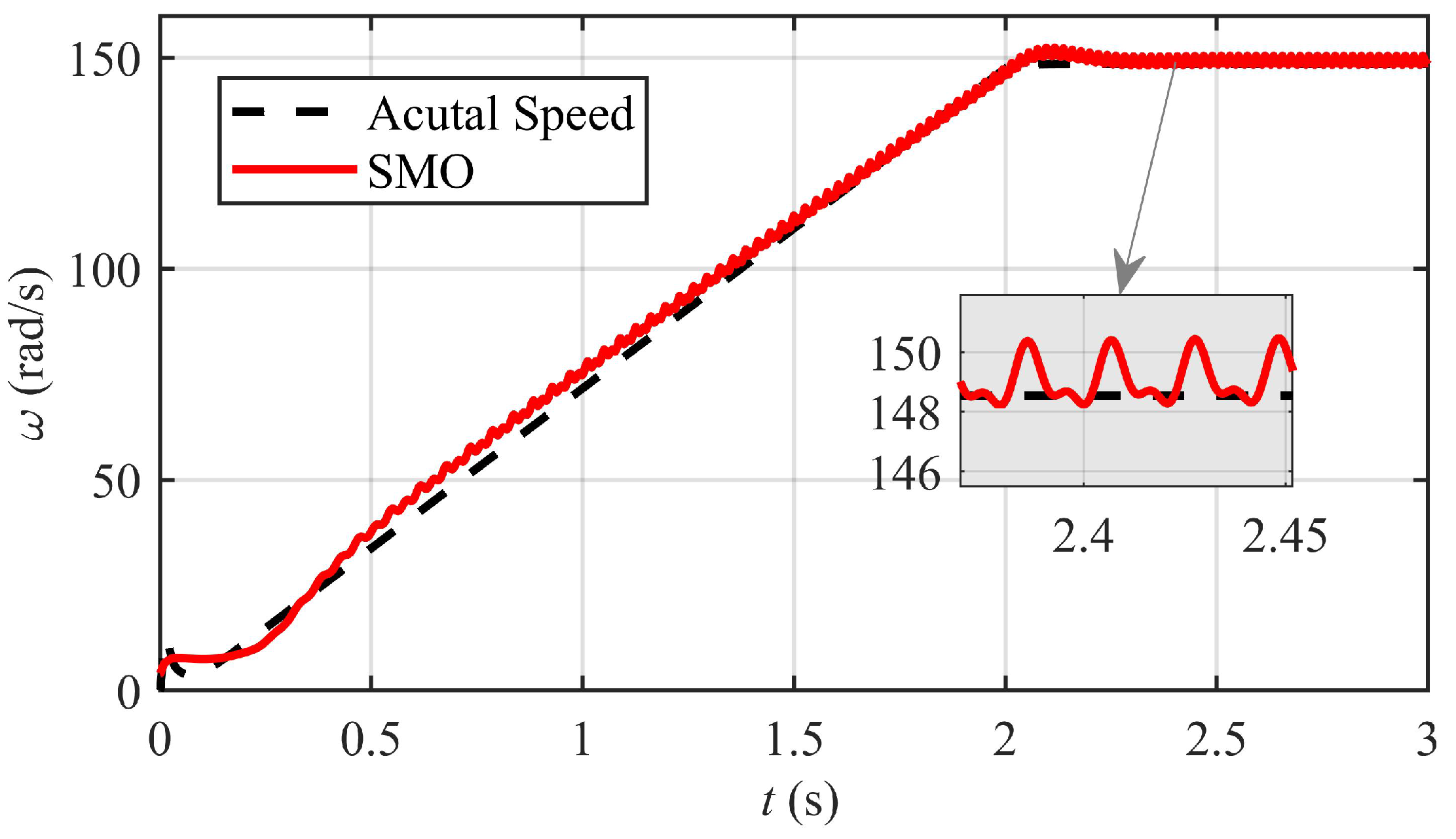
7.2. Sliding Mode Observer

Simulation-based results are given to prove and validate the performance of SMO design using the magnetizing currents of IM designed by Vieira et al. in [19]. The proposed system architecture consists of a 4 pole, 2.4 kW IM with a nominal voltage rating of 460 V (L-L, RMS). The motor parameters are L r = 0.52   H ,   L s = 0.55   H ,   L m = 0.41   H ,   R s = 2.3 Ω and R r = 2.77 Ω . In the speed estimation test, the rotor speed reference ( ω r * ) varies from 0 to 100 rad/s. The training inputs to the GPR network are given in Figure 4. The response of the SMO based rotor speed is depicted in Figure 5, verifies the estimated rotor speed convergence to the actual rotor speed and tracking of reference rotor speed. The chattering noise deters the efficient convergence of the speed observer designed in [19]. It is inhibited very well with the observer designed in this paper. The SMO-based estimated speed is given in Figure 5.
On the basis of the variable structure of the SM theory, the sliding surface is selected as:
S i ( t ) = I ^ s I s
where I ^ s = i ^ α , i ^ β are the estimated stator current values and I s = i α , i β are the actual stator current values. Based on the IM stator current determined in (5), the SMO is presented as:
i ^ α = L m 2 α r + L r R s ε L m i ^ α + L r L m v s α + α r φ α + Z α i ^ β = L m 2 α r + L r R s ε L m i ^ β + L r L m v s β + α r φ β + Z β
where Z α = K sgn i ^ α i α and Z β = K sgn i ^ β i β . Using (46), the Lyapunov stability theorem, the method followed in [19], and solving for estimated speed, we determine the required speed, which is given by:
ω ^ r = Z ¯ α e q Z β e q p L m α r i β Z ¯ α e q Z ¯ β e q Z α e q + p L m α r i β Z ¯ β e q ω ^ r = Z ¯ α e q Z β e q p L m α r i β Z ¯ α e q Z ¯ β e q Z α e q + p L m α r i β Z ¯ β e q d t
where
Z ¯ α e q = Z ^ α e q Z α e q Z ¯ β e q = Z ^ β e q Z β e q ω ¯ r = ω ^ r ω ˙ r

7.3. GPR Model-Based Speed Estimation

In this case, we analyze and display the performance of the speed estimation method using regular GPR. The estimated speed is achieved through Regular GPR, and the actual speed is shown in Figure 6a. Relatively good accuracy is achieved with RMSE = ‘0.3808’%. The RMSE, ITSE, and ISE of the different proposed methods show the advantage of GPR-based methods over non-probabilistic and non-linear speed estimation methods such as SMO. The RMSE performance of the different observers proposed in this paper using the input dataset is given in Table 2. Performance evaluation of recurrent GPR is presented in this case. The estimated speed using the recurrent GPR method and actual speed is shown in Figure 6b.
The result of the AR-GPR method of the speed estimation method is shown in Figure 6c, along with the actual speed. The performance indices graphs are shown in Figure 7 and Figure 8 illustrates that this method provides improved speed estimates compared to the regular GPR with the RMSE of ‘0.296’%. The recurrent GPR integrates the effect of present and past speed into the model. The ISE, ITSE, and RMSE illustrate that the autoregressive GPR technique improves the accuracy of speed estimation and leads to a much smoother motor speed. Mainly, the RMSE is ‘0.14’%, which is almost a perfect fit with the actual speed.
Some of the vital performance evaluation parameters are ISE and ITSE. The ISE and ITSE for the proposed observers are shown in Figure 7 and Figure 8, respectively. The ISE and ITSE for the proposed autoregressive GPR is minimum and nearly reaches zero. These performance indices validate the accurate speed estimation capability of the proposed technique.

7.4. Performance Evaluation of ST-FOSMC under Various Test Cases

The performance comparison of the proposed control scheme using the GPR-based speed observer is validated by different tests, including (a) electrical faults incorporation with load disturbance, (b) parameter perturbation with load disturbance, and (c) under-voltage with load disturbance. In the simulation evaluation, a reference speed ranging from 200 rad/s to −200 rpm was given. The response of the PI, SMC, and ST-FOSMC is given in Figure 9. It can be seen from Figure 9 that the proposed ST-FOSMC can track the reference speed faster and more precisely compared to PI and SMC control paradigms. The chattering elimination capability of the proposed control scheme is also evident, as SMC offers much chattering. In contrast, PI is converging much slower with a huge overshoot of 55 rad/s. The SMC control has an overshoot of 2 rad/s, whereas the proposed ST-FOSMC has smooth convergence with zero overshoot.
The sliding surfaces for PI, SMC, and proposed technique are shown in Figure 10. The SMC shows a lot of ripples, whereas the ST-FOSMC almost eliminates the oscillations, ensuring the smooth performance of the proposed ST-FOSMC. To verify the disturbance rejection capabilities of the proposed control paradigms, a full load was applied, and then for the rest of the time, it was halved at t = 1 s.
The robustness of the PI, SMC, and ST-FOSMC control paradigms to parameter variations were validated by varying the rotor resistance from rated resistance to 120%, 150%, and 200%. The PI controller has slow convergence and high transient oscillations, as shown in Figure 11a. The speed waveform for SMC under such conditions is shown in Figure 11b. The SMC is robust compared to the PI controller and shows fast convergence, less steady-state error, and transient oscillations. The speed response of proposed ST-FOSMC is shown in Figure 11c. The ST-FOSMC results validate that the proposed scheme is robust and insensitive to the load disturbance and parameter variation with fast settling time and minor steady-state error. The results show that the PI controller had slow convergence and high transient oscillations. On the other hand, the SMC controller demonstrated better robustness compared to the PI controller, with faster convergence, reduced steady-state error, and less transient oscillations. Moreover, the proposed ST-FOSMC controller was found to be highly robust and insensitive to load disturbances and parameter variations. The ST-FOSMC controller exhibited fast settling time and minor steady-state error, which makes it suitable for practical applications.
The dynamic performance and stability of a controller must be evaluated using electrical faults, as IM is mostly exposed to electrical faults perturbations. The various control schemes were subjected to different electrical faults, including single-phase, under-voltage, and over-voltage. The phase “a” was opened for 200 ms at t = 1 s, and the response of the control paradigm is shown in Figure 12a. The overshoot provided by the PI controller was 17 rad/s after fault incorporation, while the undershoot for PI was 13 rad/s. The SMC and ST-FOSMC provided almost the same response to the electrical fault. In this case, the average overshoot was 10 rad/s, whereas the undershoot was 10.2 rad/s. Furthermore, the PI settled after 1.8 s, whereas the SMC and ST-FOSMC settled at 1.4 s with negligible oscillations.
The motor was subjected to under-voltage and overvoltage to investigate the robustness of control strategies against electrical faults. Initially, the three-phase voltage was increased to 150% of the nominal value, and then the voltage was decreased to 50% of the nominal voltage.
The speed response for overvoltage and under-voltage is shown in Figure 12b,c, respectively. At t = 1 s, the PI scheme shows an overshoot of 9.8 rad/s, undershoot of 10 rad/s, and settling time of t = 1.65 s for the overvoltage scenario. In contrast, it showed undershoot and overshoot of 10 rad/s and 35 rad/s, respectively, and settling time of t = 1.8 s for the under-voltage scenario followed by bulky transients. The ST-FOSMC control paradigm response is almost similar to SMC in this case. The SMC provided an overshoot of 7.5 rad/s and undershoot of 7 rad/s for the overvoltage case, whereas the ST-FOSMC provided an overshoot of 7 rad/s and undershoot of 5.5 rad/s, as shown in Figure 12b. Similarly, for the under-voltage case, the SMC provided an overshoot of 20 rad/s that is almost like the proposed ST-FOTSMC, whereas the SMC provided an undershoot of 13 rad/s and that of ST-FOTMSC is 11 rad/s, as shown in Figure 12c. Hence, it can be concluded that the proposed ST-FOSMC can eliminate the chattering problem in conventional SMC and robustness problems in conventional PI, improving the inherent robustness of SMC.

8. Conclusions

A super-twisting algorithm based fractional-order sliding mode control (ST-FOSMC) is presented in this paper. The fractional calculus-based surface has been incorporated into the super-twisting algorithm-based sliding mode control (SMC). The proposed control scheme showed superior performance to the conventional PI and SMC in terms of speed convergence and robustness against load and fault perturbations. Specifically, the ST-FOSMC demonstrated a faster settling time than PI by 22.20% and SMC by 15.40% and exhibited 50% and 60% lower steady-state error than PI and SMC, respectively. Furthermore, the ST-FOSMC showed robustness to electrical faults, such as under-voltage, over-voltage, and single-phase faults, providing significantly lower overshoot and undershoot than PI and SMC, along with negligible oscillations. Speed observers based on regular GPR, recurrent GPR, and autoregressive GPR are also designed to control induction motor using simulated datasets, including the current and voltage values of the stator. AR-GPR guaranteed smooth speed estimates compared to sliding mode observers, regular GPR, and recurrent GPR. The performance of the proposed AR-GPR method was compared with regular GPR and showed improved speed estimates with a RMSE of 0.296%. Furthermore, the ISE and ITSE performance indices validated the accurate speed estimation capability of the proposed technique. The proposed speed control and estimation schemes proved to be an efficient choice for a three-phase drive system. In future works, the proposed control and estimations scheme will be implemented using an experimental workbench to testify it for practical implementation. Moreover, the proposed control scheme can be further enhanced by including a tuning mechanism based on artificial intelligence techniques. The adaptive mechanism can also be incorporated to calculate the fractional-order values used in the sliding surface of the proposed control schemes.

Author Contributions

Conceptualization, I.S.; Methodology, I.S.; Software, I.S., S.U. (Shafaat Ullah) and S.U. (Shafqat Ullah); Validation, I.S., S.U. (Shafaat Ullah) and S.S.H.B.; Formal Analysis, J.-S.R.; Investigation, N.A. and M.S. All authors have read and agreed to the published version of the manuscript.

Funding

This work was supported by the National Research Foundation of Korea (NRF) grant funded by the Korea government(MSIT) (No. NRF-2022R1A2C2004874). This work was supported by the Korea Institute of Energy Technology Evaluation and Planning (KETEP) and the Ministry of Trade, Industry & Energy(MOTIE) of the Republic of Korea (No. 20214000000280).

Data Availability Statement

Not applicable.

Conflicts of Interest

The authors have no conflict of interest.

References

  1. Lanusse, P.; Oustaloup, A.; Sabatier, J. Robust factional order PID controllers: The first generation CRONE CSD approach. In Proceedings of the ICFDA’14 International Conference on Fractional Differentiation and Its Applications 2014, Catania, Italy, 23–25 June 2014; pp. 1–6. [Google Scholar]
  2. Zhang, B.; Pi, Y. Robust fractional order proportion-plus-differential controller based on fuzzy inference for permanent magnet synchronous motor. IET Control Theory Appl. 2012, 6, 829–837. [Google Scholar] [CrossRef]
  3. Viola, J.; Angel, L.; Sebastian, J. Design and robust performance evaluation of a fractional order PID controller applied to a DC motor. IEEE/CAA J. Autom. Sin. 2017, 4, 304–314. [Google Scholar] [CrossRef]
  4. Efe, M.Ö. Fractional fuzzy adaptive sliding-mode control of a 2-DOF direct-drive robot arm. IEEE Trans. Syst. Man Cybern. Part B 2008, 38, 1561–1570. [Google Scholar] [CrossRef]
  5. Ladaci, S.; Charef, A. On fractional adaptive control. Nonlinear Dyn. 2006, 43, 365–378. [Google Scholar] [CrossRef]
  6. Calderon, A.J.; Vinagre, B.M.; Feliu, V. Fractional order control strategies for power electronic buck converters. Signal Process. 2006, 86, 2803–2819. [Google Scholar] [CrossRef]
  7. Delavari, H.; Ghaderi, R.; Ranjbar, A.; Momani, S. Fuzzy fractional order sliding mode controller for nonlinear systems. Commun. Nonlinear Sci. Numer. Simul. 2010, 15, 963–978. [Google Scholar] [CrossRef]
  8. Abdelhamid, D.; Bouden, T.; Boulkroune, A. Design of fractional-order sliding mode controller (FSMC) for a class of fractional-order non-linear commensurate systems using a particle swarm optimization (PSO) algorithm. J. Control Eng. Appl. Inform. 2014, 16, 46–55. [Google Scholar]
  9. Cao, D.; Fei, J. Adaptive fractional fuzzy sliding mode control for three-phase active power filter. IEEE Access 2016, 4, 6645–6651. [Google Scholar] [CrossRef]
  10. Zhong, X.; Shao, X.; Li, X.; Ma, Z.; Sun, G. Fractional order adaptive sliding mode control for the deployment of space tethered system with input limitation. IEEE Access 2018, 6, 48958–48969. [Google Scholar] [CrossRef]
  11. Sami, I.; Khan, B.; Asghar, R.; Mehmood, C.A.; Ali, S.M.; Ullah, Z.; Basit, A. Sliding Mode-Based Model Predictive Torque Control of Induction Machine. In Proceedings of the 2019 International Conference on Engineering and Emerging Technologies (ICEET), Lahore, Pakistan, 21–22 February 2019; pp. 1–5. [Google Scholar]
  12. Song, S.; Zhang, B.; Song, X.; Zhang, Y.; Zhang, Z.; Li, W. Fractional-order adaptive neuro-fuzzy sliding mode H control for fuzzy singularly perturbed systems. J. Frankl. Inst. 2019, 356, 5027–5048. [Google Scholar] [CrossRef]
  13. Xu, D.; Wang, B.; Zhang, G.; Wang, G.; Yu, Y. A review of sensorless control methods for AC motor drives. CES Trans. Electr. Mach. Syst. 2018, 2, 104–115. [Google Scholar] [CrossRef]
  14. Ullah, N.; Ali, M.A.; Ibeas, A.; Herrera, J. Adaptive fractional order terminal sliding mode control of a doubly fed induction generator-based wind energy system. IEEE Access 2017, 5, 21368–21381. [Google Scholar] [CrossRef]
  15. Singh, S.; Tiwari, A. Various techniques of sensorless speed control of PMSM: A review. In Proceedings of the 2017 Second International Conference on Electrical, Computer and Communication Technologies (ICECCT), Coimbatore, India, 22–24 February 2017; pp. 1–6. [Google Scholar]
  16. Yan, Z.; Jin, C.; Utkin, V. Sensorless sliding-mode control of induction motors. IEEE Trans. Ind. Electron. 2000, 47, 1286–1297. [Google Scholar]
  17. Cherifi, D.; Miloud, Y. Technology, Online Stator and Rotor Resistance Estimation Scheme Using Sliding Mode Observer for Indirect Vector Controlled Speed Sensorless Induction Motor. Am. J. Comput. Sci. 2019, 2, 1–8. [Google Scholar] [CrossRef]
  18. Guezmil, A.; Berriri, H.; Pusca, R.; Sakly, A.; Romary, R.; Mimouni, M.F. High order sliding mode observer-based backstepping fault-tolerant control for induction motor. Asian J. Control 2019, 21, 33–42. [Google Scholar] [CrossRef]
  19. Sami, I.; Ullah, S.; Basit, A.; Ullah, N.; Ro, J.S. Integral super twisting sliding mode based sensorless predictive torque control of induction motor. IEEE Access 2020, 8, 186740–186755. [Google Scholar] [CrossRef]
  20. Rasmussen, H.; Vadstrup, P.; Borsting, H. Full adaptive backstepping design of a speed sensorless field oriented controller for an induction motor. In Proceedings of the Conference Record of the 2001 IEEE Industry Applications Conference. 36th IAS Annual Meeting (Cat. No. 01CH37248), Chicago, IL, USA, 30 September–4 October 2001; Volume 4, pp. 2601–2606. [Google Scholar]
  21. Alonge, F.; D’Ippolito, F.; Sferlazza, A. Sensorless control of induction-motor drive based on robust Kalman filter and adaptive speed estimation. IEEE Trans. Ind. Electron. 2013, 61, 1444–1453. [Google Scholar] [CrossRef]
  22. Yin, Z.; Li, G.; Zhang, Y.; Liu, J.; Sun, X.; Zhong, Y. A speed and flux observer of induction motor based on extended Kalman filter and Markov chain. IEEE Trans. Power Electron. 2016, 32, 7096–7117. [Google Scholar] [CrossRef]
  23. Yu, H.X.; Hu, J.T. Speed and load torque estimation of induction motors based on an adaptive extended Kalman filter. In Advanced Materials Research; Trans Tech Publ.: Stafa-Zurich, Switzerland, 2012; Volume 433, pp. 7004–7010. [Google Scholar]
  24. Yildiz, R.; Barut, M.; Zerdali, E.; Inan, R.; Demir, R. Load torque and stator resistance estimations with unscented Kalman filter for speed-sensorless control of induction motors. In Proceedings of the 2017 International Conference on Optimization of Electrical and Electronic Equipment (OPTIM) & 2017 Intl Aegean Conference on Electrical Machines and Power Electronics (ACEMP), Brasov, Romania, 25–27 May 2017; pp. 456–461. [Google Scholar]
  25. Jannati, M.; Idris, N.; Aziz, M. Speed sensorless fault-tolerant drive system of 3-phase induction motor using switching extended kalman filter. TELKOMNIKA Indones. J. Electr. Eng. 2014, 12, 7640–7649. [Google Scholar] [CrossRef]
  26. Bogosyan, S.; Barut, M.; Gokasan, M. Braided extended Kalman filters for sensorless estimation in induction motors at high-low/zero speed. IET Control Theory Appl. 2007, 1, 987–998. [Google Scholar] [CrossRef]
  27. Zerdali, E.; Barut, M. Novel version of bi input-extended Kalman filter for speed-sensorless control of induction motors with estimations of rotor and stator resistances, load torque, and inertia. Turk. J. Electr. Eng. Comput. Sci. 2016, 24, 4525–4544. [Google Scholar] [CrossRef]
  28. Silva, W.L.; Lima, A.M.N.; Oliveira, A. Speed estimation of an induction motor operating in the nonstationary mode by using rotor slot harmonics. IEEE Trans. Instrum. 2014, 64, 984–994. [Google Scholar] [CrossRef]
  29. Karanayil, B.; Rahman, M.F.; Grantham, C. Online stator and rotor resistance estimation scheme using artificial neural networks for vector controlled speed sensorless induction motor drive. IEEE Trans. Ind. Electron. 2007, 54, 167–176. [Google Scholar] [CrossRef]
  30. Jahangir, M.; Afzal, H.; Ahmed, M.; Khurshid, K.; Nawaz, R. An expert system for diabetes prediction using auto tuned multi-layer perceptron. In Proceedings of the 2017 Intelligent Systems Conference (IntelliSys), London, UK, 7–8 September 2017; pp. 722–728. [Google Scholar]
  31. Jahangir, M.; Afzal, H.; Ahmed, M.; Khurshid, K.; Amjad, M.F.; Nawaz, R.; Abbas, H. Auto-MeDiSine: An auto-tunable medical decision support engine using an automated class outlier detection method and AutoMLP. Neural Comput. Appl. 2019, 32, 2621–2633. [Google Scholar] [CrossRef]
  32. Ayyaz, S.; Qamar, U.; Nawaz, R. HCF-CRS: A Hybrid Content based Fuzzy Conformal Recommender System for providing recommendations with confidence. PLoS ONE 2018, 13, e0204849. [Google Scholar] [CrossRef]
  33. Brandstetter, P.; Kuchar, M. Sensorless control of variable speed induction motor drive using RBF neural network. J. Appl. Log. 2017, 24, 97–108. [Google Scholar] [CrossRef]
  34. Song, S.; Zhang, B.; Xia, J.; Zhang, Z. Adaptive backstepping hybrid fuzzy sliding mode control for uncertain fractional-order nonlinear systems based on finite-time scheme. IEEE Trans. Syst. Man Cybern. Syst. 2018, 50, 1559–1569. [Google Scholar] [CrossRef]
  35. Zhu, S.; Luo, X.; Xu, Z.; Ye, L. Seasonal streamflow forecasts using mixture-kernel GPR and advanced methods of input variable selection. Hydrol. Res. 2019, 50, 200–214. [Google Scholar] [CrossRef]
Figure 1. Prominent SMC variants in literature.
Machines 11 00584 g001
Figure 2. The Proposed Closed-loop Motor Drive Control Structure.
Machines 11 00584 g002
Figure 3. Ar-GPR model for speed estimation.
Machines 11 00584 g003
Figure 4. Training Inputs.
Machines 11 00584 g004
Figure 5. SMO based estimated speed.
Machines 11 00584 g005
Figure 6. GPR based observer performance. (a) Regular GPR. (b) Recurrent GPR. (c) Auto-Regressive GPR.
Machines 11 00584 g006
Figure 7. Integral Square Error (ISE).
Machines 11 00584 g007
Figure 8. Integral time Square Error (ITSE).
Machines 11 00584 g008
Figure 9. Speed response of PI, SMC, and the proposed ST-FOSMC.
Machines 11 00584 g009
Figure 10. Sliding Surfaces comparison of PI, SMC, and ST-FOSMC.
Machines 11 00584 g010
Figure 11. Controllers performance under parametric variations. (a) PI response Under parameter Variation. (b) SMC response Under Parameter Variation. (c) Proposed ST-FOSMC response Under Parameter Variation.
Machines 11 00584 g011
Figure 12. Controllers performance under faults. (a) Single-phase Fault. (b) Over Voltage. (c) Under Voltage.
Machines 11 00584 g012
Table 1. Induction motor tuning parameters.
IM ParametersValues
Rated Power 3 HP / 2.4 kW
Phases3
Line Voltage 460 V ( L L , rms )
System Frequency 60 Hz
Full Load Slip 1.72 %
Number of Poles4
Switching Frequency 20 kHz
Stator Resistance 1.7 Ω
Stator Leakage Resistance 5.25 Ω
Rotor Resistance 1.34 Ω
Rotor Leakage Resistance 4.57 Ω
Moment of Inertia 70 kg · m 2
Mutual Inductance 139 Ω
Full Load Current 4 A
Full Load Speed 1750 rpm
Table 2. Control and Observer Parameters.
ParametersValuesRMSE (%)
α 0.9
β 1.1
c50.1
c64
l d for Regular GPR2.5 for V(k), 160 for I(k)0.3808
4.5 for V(k), 260 for I(k),
l d for AR-GPR2.1 for V(k-1), 200 for I(k-1),0.14
300 for ω ( k 1 )
K101.2
Disclaimer/Publisher’s Note: The statements, opinions and data contained in all publications are solely those of the individual author(s) and contributor(s) and not of MDPI and/or the editor(s). MDPI and/or the editor(s) disclaim responsibility for any injury to people or property resulting from any ideas, methods, instructions or products referred to in the content.

