
Feature-Based MPPI Control with Applications to Maritime Systems †

1
Institute of System Dynamics, HTWG Konstanz—University of Applied Sciences, 78462 Konstanz, Germany
2
Department of Microsystems Engineering (IMTEK), University of Freiburg, 79110 Freiburg, Germany
3
Department of Mathematics, University of Freiburg, 79110 Freiburg, Germany
*
Author to whom correspondence should be addressed.
†
This paper is an extended version of our paper published in Proceedings of the 6th IEEE Conference on Control Technology and Applications (CCTA), Trieste, Italy, 22–25 August 2022, with the title “Feature-Based Proposal Density Optimization for Nonlinear Model Predictive Path Integral Control”.
Machines 2022, 10(10), 900; https://doi.org/10.3390/machines10100900
Submission received: 13 September 2022
/
Revised: 27 September 2022
/
Accepted: 29 September 2022
/
Published: 6 October 2022
(This article belongs to the Special Issue Nonlinear Control Applications and New Perspectives)
Abstract
:In this paper, a novel feature-based sampling strategy for nonlinear Model Predictive Path Integral (MPPI) control is presented. Using the MPPI approach, the optimal feedback control is calculated by solving a stochastic optimal control (OCP) problem online by evaluating the weighted inference of sampled stochastic trajectories. While the MPPI algorithm can be excellently parallelized, the closed-loop performance strongly depends on the information quality of the sampled trajectories. To draw samples, a proposal density is used. The solver’s and thus, the controller’s performance is of high quality if the sampled trajectories drawn from this proposal density are located in low-cost regions of state-space. In classical MPPI control, the explored state-space is strongly constrained by assumptions that refer to the control value’s covariance matrix, which are necessary for transforming the stochastic Hamilton–Jacobi–Bellman (HJB) equation into a linear second-order partial differential equation. To achieve excellent performance even with discontinuous cost functions, in this novel approach, knowledge-based features are introduced to constitute the proposal density and thus the low-cost region of state-space for exploration. This paper addresses the question of how the performance of the MPPI algorithm can be improved using a feature-based mixture of base densities. Furthermore, the developed algorithm is applied to an autonomous vessel that follows a track and concurrently avoids collisions using an emergency braking feature. Therefore, the presented feature-based MPPI algorithm is applied and analyzed in both simulation and full-scale experiments.
1. Introduction
Recently, empowered by the progresses in efficiency of optimization algorithms and the available computing power, sample-based nonlinear model predictive control (NMPC) approaches can be used to solve nonlinear stochastic OCP in real time [1]. Using the path integral control framework [2], the stochastic HJB equation that corresponds to a restricted class of stochastic OCPs can be transformed into a linear partial second-order differential equation [3]. This class is characterized by arbitrary but input affine dynamics, containing additive white Gaussian noise (AWGN) at the inputs, and the cost function is only restricted to be quadratic in the controls [4]. According to [3], a Feynman–Kac path integral can be used to express the solution for both, the optimal controls and the optimal value function. Thus, the solution of the transformed stochastic HJB is formulated as a conditional expectation value with respect to the system dynamics. As a result, the optimal control can be estimated using Monte Carlo methods drawing samples of stochastic trajectories [5]. While in general the resulting optimal feedback control function has an unknown structure, there are different approaches for its representation. Besides reinforcement learning (RL) approaches based on offline learning a parametrized policy [6,7], NMPC has become the de-facto technological standard [8,9]. Based on path integrals, a new type of sample-based NMPC algorithm was presented in [8]. Using a free energy definition described in [10] and [11], the input affine requirement is completely removed by [4]. Because MPPI is based on Monte Carlo simulation, the information content of the drawn samples is highly dependent on the proposal density [12,13]. Due to this fact, the system’s performance can be significantly improved by provisioning a good proposal density. While recently in [14] a robust MPPI version, in [15] a covariance steering approach and in [16] a learning-based algorithm are introduced, in this paper, a novel feature-based MPPI extension is presented. In Section 2, the basics of the MPPI approach are described. This is followed by the derivation of a feature-based extension of the MPPI algorithm in Section 3. In Section 4, an application scenario is defined containing the equations of motions of a vessel and cost functions, which are combined as an OCP. Furthermore, an emergency braking feature is defined. In Section 5, the controller design is presented including the architecture, the controller parameters and the cost function parameters. A comparison of usual MPPI control and its feature-based extension in a simulation environment is given in Section 6. In Section 7, full-scale experiments with the research vessel Solgenia are used to compare the MPPI algorithm and its feature-based extension. This is followed by the conclusions of this paper including ideas for future work in Section 8.
2. Model Predictive Path Integral Control
Recently, a sample-based NMPC algorithm was derived by [4] using the path integral framework. This so-called MPPI approach calculates the optimal control inputs by numerically solving the time-discrete nonlinear stochastic OCP
in real time, where denotes the time-discrete nonlinear system dynamics of the stochastic system state , and the actual system input denoted by that is given by the commanded system’s input with time discrete AWGN with covariance matrix . The so-called temperature of the stochastic system is denoted by . The objective function is given by the expected value of the terminal costs denoted by , the instantaneous stage costs denoted by and a quadratic input term with weighting matrix . The objective function to be minimized in (1a) evaluates the expected costs subject to the commanded system inputs under the measurement distribution corresponding to the probability density function (PDF)
where denotes the sequence of actual input values. The distribution of the controlled system denoted by corresponds to an open-loop sequence of manipulated variables for . According to [17], the expectation value under a measurement is defined as , where denotes a scalar function. In this section, the basics of this novel algorithm are described before it will be extended in the next section. According to [4], the density function of the uncontrolled system denoted by with zero input leads to the PDF
An initial state and a realized sequence of input values can be uniquely assigned to a trajectory without stochastic influence by recursively applying (1b). Introducing the cumulated state-dependent path costs according to [4], the value function of the OCP (1a) is given by
with respect to the uncontrolled dynamics [4]. To express the value function with respect to , the likelihood ratio must be introduced, which yields
Applying Jensen’s inequality according to [4] yields
where the bound is tight with
where denotes a normalization constant. In [4], it is shown that the associated optimal control values are given by
where denotes the Kullback–Leibler divergence, and denotes the abstract optimal distribution. According to [4], the optimal input is given by
minimizing (1a), where denotes the image of the sample space, and the importance weighting
can be calculated using the PDFs (2), (3) and (7). Using Monte Carlo simulation, (9a) can be estimated via the iterative update law
where N samples are drawn from the system dynamics (1b) with the commanded control input sequence The iterative procedure described in Algorithm 1 is used to estimate the optimal commanded control input, and to improve the required importance sample distribution simultaneously.
| Algorithm 1 Optimize Control Sequence (OCS) acc. to [4] |
| Input:: Transition model; |
| K: Number of samples; |
| T: Number of timesteps; |
| : Initial control sequence; |
| : Recent state estimate; |
| : Control hyper-parameters; |
| Output:: Optimized control sequence |
| : Average costs; |
| 1: for do |
| 2: ; |
| 3: Sample ; |
| 4: ; |
| 5: for do |
| 6: ; |
| 7: ; |
| 8: end for |
| 9: ; |
| 10: end for |
| 11: ; |
| 12: ; |
| 13: for do |
| 14: ; |
| 15: end for |
| 16: for do |
| 17: ; |
| 18: end for |
| 19: ; |
| 20: return and |
3. Extension to Feature-Based Proposal Density
In this section, the exploration problem of standard MPPI control is described, the idea of feature-based extension is presented and the resulting feature-based MPPI algorithm is presented.
3.1. Exploration Problem of Classical MPPI Control
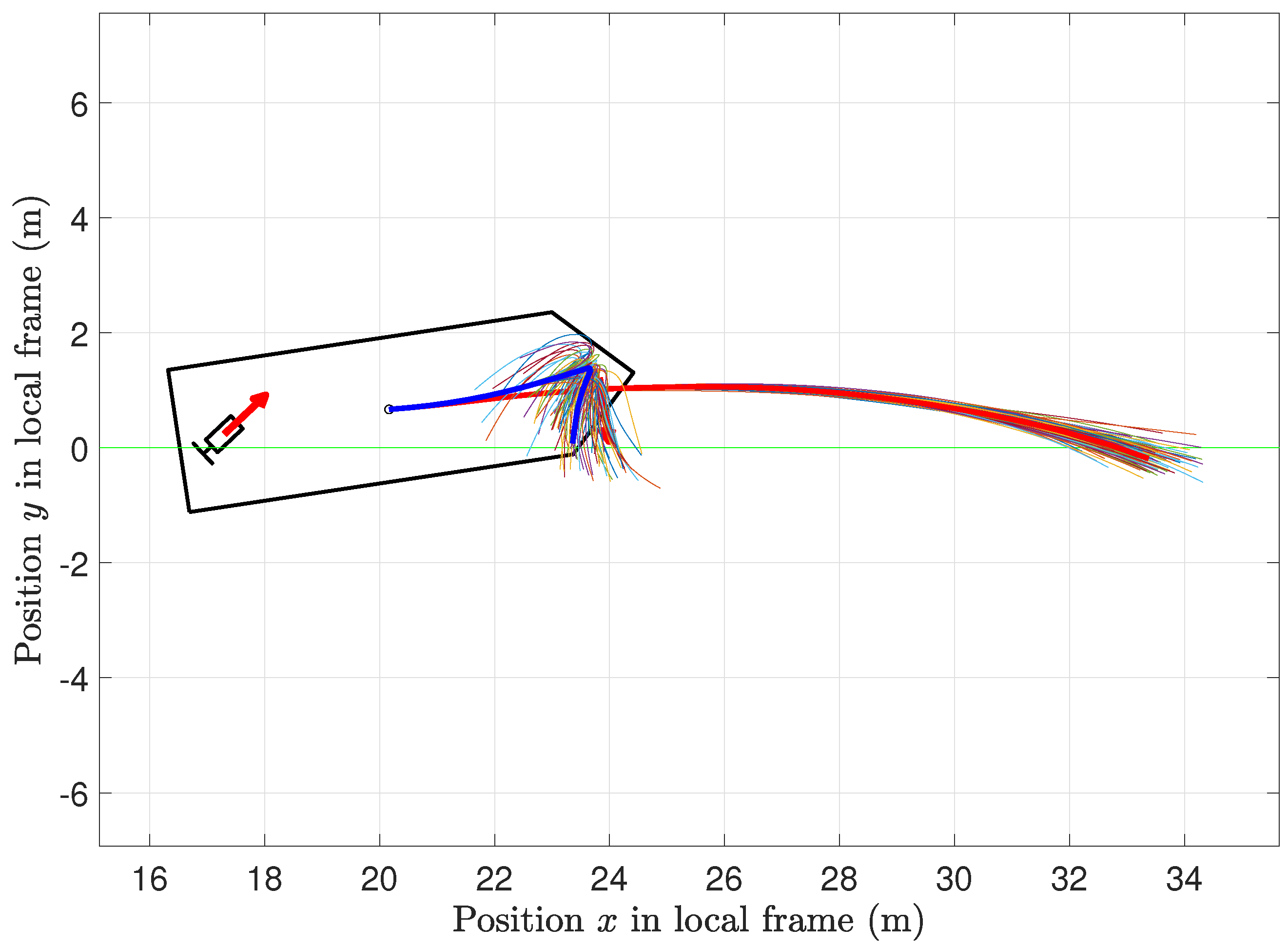
To improve the sampling efficiency, both the value function (5) and the optimal control sequence (9b) can be calculated by sampling trajectories under the probability measure with the proposal PDF (2). Due to the restrictive assumption , the proposal PDF is only parametrized by a sequence of inputs . The sampling efficiency is dependent on the quality of the proposal density [13]. In [4], the recent estimate of the optimal control sequence is used to determine the proposal PDF for the next sampling iteration. The objective function (1a) is not necessarily convex. Using an infinite number of samples, the MPPI algorithm is a global minimizer. However, due to a finite number of drawable samples, the explored state-space is concentrated around the last approximation. In order not to remain in a local minimum, the explored state-space must be enlarged. An exemplary possibility to enlarge the explored state–space is shown in Figure 1.
3.2. Feature-Based Extension of the Search Space
An enlargement of the explored state-space is possible by introducing an additional feature-based proposal density to draw a part of the samples from. Therefore, a feature is implicitly defined by solving the artificially designed OCP
where denotes the terminal costs of a feature and denotes the instantaneous costs of a feature. Thus, the feature-based proposal density is given by
parametrized by a sequence of inputs . Analogous to the previous section, the stochastic OCP (12a) can be solved by using the MPPI algorithm.
3.3. Resulting Feature-Based MPPI Algorithm
The resulting feature-based MPPI algorithm is presented in Algorithm 2. First, the control sequence is optimized using Algorithm 1, and the predicted costs are evaluated. Then, all feature control sequences are improved, and their performances regarding the main cost function are evaluated. The best control sequence is chosen to be the main control sequence. Then, the first element of the control sequence is applied. Subsequently, the sequence is shifted, and the last element is initialized. Note: In the implementation, lines 4 and 5 can be combined to reduce the computational effort.
| Algorithm 2 Feature-Based MPPI Control |
| Input:: Transition model; |
| K: Number of samples; |
| T: Number of timesteps; |
| : Initial control sequence; |
| : Recent state estimate; |
| : Control hyper-parameters; |
| I: Number of features with feature index ; |
| : Initial control sequence of feature; |
| : State dependent costs of feature; |
| : Number of features samples; |
| 1: while Controller is active do |
| 2: |
| 3: for do |
| 4: |
| 5: |
| 6: end for |
| 7: |
| 8: |
| 9: SendToActuator; |
| 10: for do |
| 11: |
| 12: end for |
| 13: |
| 14: end while |
4. Maritime Application Scenario
Autonomous mobility of maritime systems is a central problem of our time. Due to advances in science and technology, the requirements for the performance are constantly increasing. For example, recent publications such as [18,19,20] show how NMPC algorithms are used in the maritime environment to solve complex control engineering problems. Moreover, algorithms in the context of RL such as Deep Q-learning [21], Deep Deterministic Policy Gradients [22] or Actor–Critic [23] are increasingly used, which achieve good results for various applications, but the majority of them are only validated in simulation. While MPPI control was used to dock a fully actuated vessel in full-scale autonomously [24], a gap in this research area is the feature-based MPPI control of an autonomous vessel for collision avoidance. In order to also being able to perform autonomous maneuvers, such as heading for a defined target outside the port, it must be ensured that the hazards during these maneuvers are minimized. As regulated by the International Regulations for Preventing Collisions at Sea (COLREG) [25], in the event of a predicted collision, it is mandatory to take evasive action. In poor visibility conditions such as fog, heavy rain or due to obstacles appearing through the water surface, there are scenarios where the vessel’s sensors will not detect potential collision partners until a short distance away. In such a scenario, using the standard MPPI approach, all sampled trajectories would result in a collision. This overloads the controller and makes it impossible to avoid a collision. Thus, the question arises how feature-based MPPI control can be applied to avoid a collision even in such a scenario. To answer the question, the feature-based MPPI control algorithm is applied in an emergency braking scenario for an autonomous vessel. In the scenario being discussed, the vessel is traveling at full speed along a predefined path, where an obstacle appears at a certain point. Therefore, the vessel has to autonomously perform a so-called last-minute maneuver to avoid a collision. To provide an overview, first the state and dynamics of the fully actuated research vessel Solgenia are presented. Then, a standard MPPI controller is parameterized, which causes the vessel to follow a predefined path. This is then extended to a feature-based MPPI controller by introducing an emergency brake feature.
4.1. Dynamics of the Vessel
In [26], a detailed description of the dynamics of the research vessel Solgenia including identification of the model parameters and the calculation of the actuator thrusts is outlined. Nevertheless, a short description of the modeling is given in the following since the model is an elementary component of the MPPI approach used in the scenario. A photography of the research vessel Solgenia is shown in Figure 2a. According to [27], the vessel’s state vector is given by a combination of the 2D pose and the velocity vector in body-fixed coordinates, shown in Figure 2b. This model was extended in [24] to also consider the dynamics of the actuators. Thus, the transfer properties of the controlled actuators can be modeled in each case by a first-order low-pass filter with an equivalent time constant , limited slope , and dead time represented by
where denotes the i-th actuator’s desired state and denotes the i-th actuator’s actual state. Thus, the actual actuator states , where the speed of the azimuth thruster (AT) is denoted by , the orientation of the AT is denoted by and denotes the speed of the bow thruster (BT), and the desired actuator states denoting the desired variables of get a part in the system state
The whole dynamic model of the vessel is given by
where in (16a) the desired variable vector includes the integral action . In (16b), the actuators’ dynamics are considered by whose components are given in (14). According to [27], the time derivative of the body-fixed velocity is implicitly described in (16c) as a function of the body-fixed velocity , the mass matrix
the Coriolis matrix
and the damping matrix
including the system parameters listed in Table 1, the input vector and disturbance vector . The kinematics Equation (16d) describes the transformation of the body-fixed velocity into local coordinates as a function of the rotation matrix . The influence of unmodeled effects and environmental disturbances are represented by the disturbance vector . The controlled force vector
depends on the geometric parameters , and and the thrusts and , shown in Figure 2b. The thrust is generated by the AT, and denotes the thrust generated by the BT. These thrust forces can be modeled according to [28] dependent on various physical constants, the body fixed velocity vector and the actual states of the actuators . Thus, the force generated by the BT is given by
where denotes a unitless constant with
denotes the density of the water, the diameter of the propeller is denoted by . Furthermore, the quadratic damping of the thrust dependent on the surge velocity component is scaled by a coefficient denoted by . Using this modeling structure, the influence of the relative speed in the axial direction of the BT is assumed to be small and hence neglected. This assumption cannot be used when modeling the force , since the relative axial velocity component of the AT is large in the given application scenario and given by
where denotes the distance between the AT and the vessel’s center of gravity (CG). According to [26], the force generated by the AT is modeled by
where denotes the AT’s diameter, and the coefficients and are given by
where denote the coefficients of the AT. The parameters identified by [26] are listed in Table 2. Note that, according to [26], the parameters and are eliminated during the evaluation phase of the identification process. For more detailed information about the dynamics, the reader is referred to [24,26,27].
4.2. Inequality Constraints
Due to the maximum speed of the actuators, two inequality constraints
are defined. By considering the actuator dynamics (14) in the model, no further inequality constraints are required.
4.3. Equality Constraints
In the treated scenario, the most important aim is to avoid collisions. In order to achieve this, first the indicator function
is defined, where is the subset of the state-space where the vessel causes a collision and is a disjoint subset. Consequently, the equality constraint to be fulfilled is given by
where only the indicator function (27) is used. In the next part, the derivation of the cost function is presented for the given scenario.
4.4. Cost Function
The instantaneous state-dependent cost function significantly governs the behavior of the controlled system, since it is used to evaluate the sampled stochastic trajectories. However, for a complex task, the stage cost function can be learned from expert behavior; using inverse reinforcement learning [29,30,31] for the given scenario, we can define the linguistic criteria for the cost function and then express them as simple equations and subsequently add them up. The vessel should move on a predefined trajectory shown in Figure 3 and should avoid collisions. This task is complicated by significant current, wind and further disturbance effects that occur when moving in the Rhine River. For a good system behavior, the vessel should meet the following criteria, which are sorted in descending order of importance:
- A collision should be prevented.
- The actuators must not be overloaded.
- The position should follow a predefined the trajectory.
- The orientation should be in line with the trajectory.
- While the surge velocity component should match a reference, the absolute value of the sway component and yaw-rate component should be minimized.
While criteria 1 and 2 are already treated introducing the inequality and equality constraints, to meet criteria 3–5, the quality of sampled trajectories is evaluated based on two parts
where denotes the position and orientation dependent costs used to meet the criteria 3 and 4, denotes the part of the cost function that is dependent on the body-fixed velocity and thus is introduced w.r.t. meeting criterion 5. In the following, the parts of the cost function (29) are presented.
4.4.1. Costs Dependent on the Position
For a clear presentation of the costs dependent on the position, these are defined in transformed local coordinates, which are generated by the linear transformation
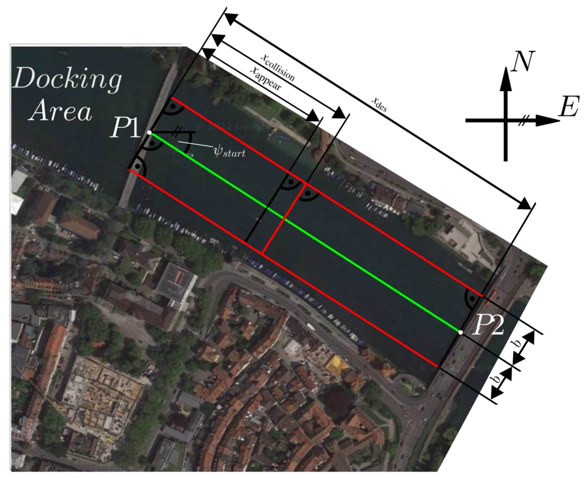
where the start orientation of the trajectory is denoted by and denotes the 2D pose located at P1 given in Table 3. Subsequently, the costs dependent on the transformed position are given by
where denote weighting coefficients, and denotes the distance between and shown in Figure 3.
4.4.2. Costs Dependent on the Velocity
The difference between the body-fixed velocity components and the desired reference velocity is penalized using
where denote the weighting coefficients. Note that this velocity dependent part of the cost function is minimized by the optimal velocity . Thus, a drifting behavior of the vessel is penalized. In the next section, the resulting problem formulation is given.
4.5. Resulting Problem Formulation
To minimize the cumulated costs (29) subject to the given dynamics (16a)–(16d), for the inequality constraints (26) and the equality constraints (28) using MPPI control, the OCP has to be formulated in the assumed structure (1a)–(1b). Consequently, the equality and inequality constraints must be considered in the cost function with
being defined, where denotes coefficients of the penalty terms. In addition, the terminal cost function must be determined. Because this function is not needed in the given scenario, it is defined as
In MPPI control according to [4], a discrete-time system dynamics with additive input noise is assumed in (1b). Therefore, the time continuous system dynamics given in (16a)–(16d) is discretized using the explicit fourth order Runge–Kutta method with a step size h. Therefore, the input signal is chosen to be piecewise constant within this step size. Consequently, the discrete-time vessel dynamics that maps a system state is given by
Finally, the assumption that the input of the system is disturbed with time discrete AWGN yields
where denotes the actual and the desired system input at time instance t. The covariance matrix of the AWGN is denoted by . Using these assumptions, the resulting stochastic OCP is given by
where the sequence of desired inputs is denoted by . In the next part, the usual MPPI approach is extended to the feature-based MPPI to improve the system’s behavior.
4.6. Feature Definition
To use the presented feature-based MPPI algorithm, at least one feature has to be chosen. As already discussed in Section 4.4, the selection of the features can be done by inverse reinforcement learning [30,31] or by the definition of a linguistic quality criterion, which is subsequently formulated mathematically. It is important to note that only well-chosen features lead to an improvement of the system’s behavior. In this context, well-chosen means that, in some cases, low-cost regions of the original cost function (33) of state-space are explored by sampling trajectories with controls, which minimizes the feature costs. Note, for the given scenario, the following linguistic quality criterion is defined: a reduction in speed can mitigate or even prevent a collision with an obstacle. For this purpose, an emergency break feature is defined by choosing
where denote the coefficients of the velocity dependent costs. Consequently, a control sequence that minimizes this feature leads to the exploration of the region of the state-space decreasing the vessel’s velocity. In the following section, the presented scenario is used to compare the performance of classical MPPI and feature-based MPPI control.
5. Controller Design
In this section, the design for both the standard MPPI controller presented in Section 2 and the feature-based MPPI controller presented in Section 3 is shown with application to maritime scenario presented in Section 4. For this purpose, the modularized and distributed control structure used is described. Note that an Unscented Kalman Filter (UKF) according to [33] is used to estimate the system state based on the sensor signals and the actuators’ states. These are controlled in subordinate control loops. This is followed by a description of how the control parameters are determined. Finally, the selection of the cost function’s coefficients is presented.
5.1. Architecture
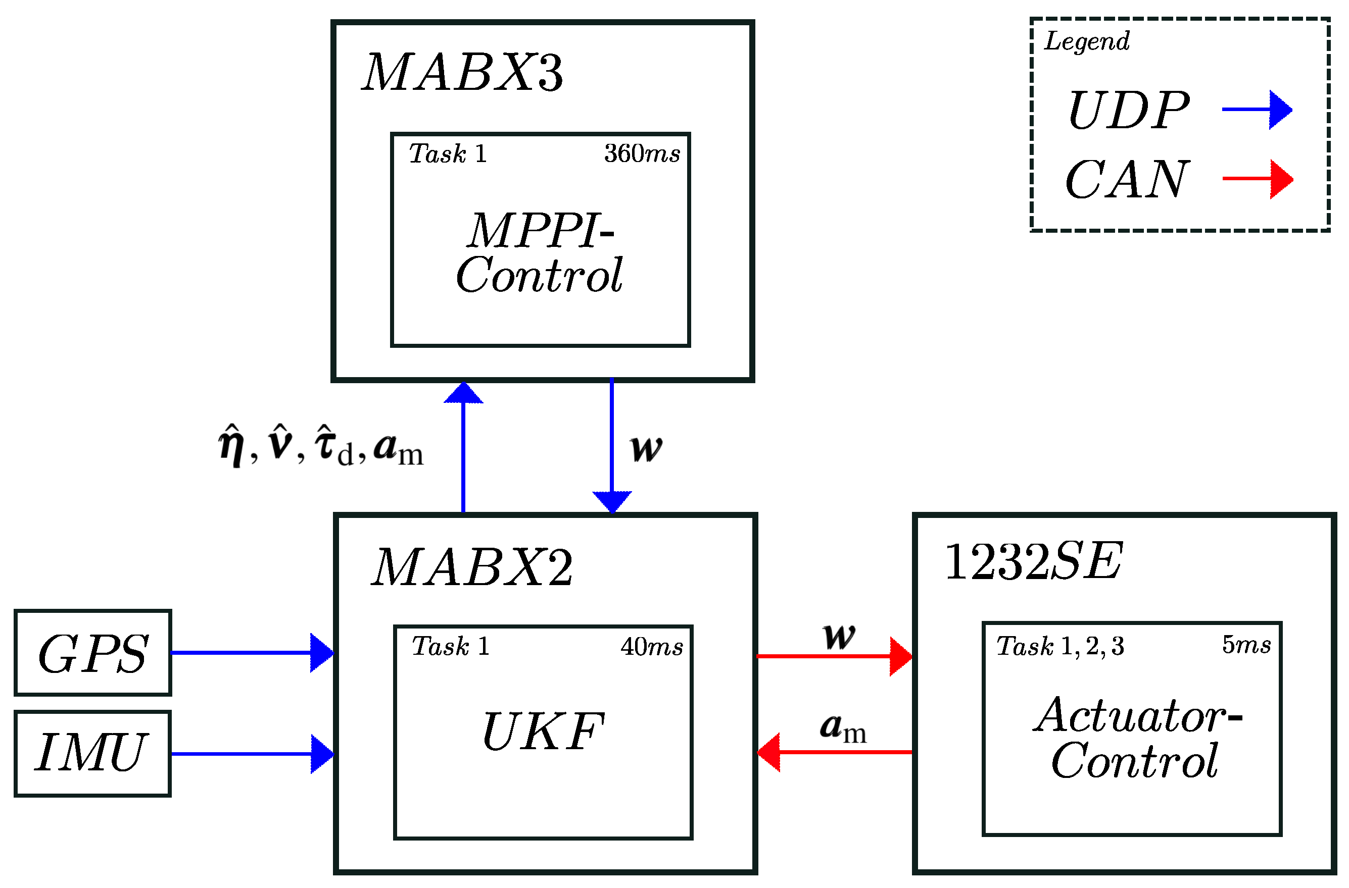
An overview of all parts of the used control architecture is given in Figure 4. The state estimation and the communication are performed by the rapid prototyping system MicroAutoBox2 (MABX2). While the supervisory MPPI algorithm is running on the MABX3, three subordinate 1232SE control units by Curtis are used to control the drives. An RTK-GPS and an IMU sensor send their measurement data to the MABX2 using a UDP protocol. Using a UKF, this information is fused with the measured actuator state to estimate the system’s 2D pose denoted by , the body-fixed velocity vector and the disturbance forces , which are sent to the MABX3 via UDP protocol. The MPPI algorithm uses the provided state estimation to calculate the desired system input . Because the system input is defined as the zero-order-hold time derivative of the desired values of the actuator control loops, an explicit Euler integrator can be used to calculate implemented on the MABX3. Subsequently, is sent via UDP protocol to the MABX2, which then provides to the subordinated actuator controllers via CAN protocol. The encoders’ measurements of are denoted by and collected with high quality; therefore, no additional signal processing is needed. The measured actuator states are sent from the encoders to the 1232SE drive controllers, which then send them via UDP to the MABX2 for state estimation.
5.2. Controller Parameters
The choice of controller parameters determines the properties of the sampled trajectories, which are realizations over . They have a significant influence on the quality of the estimation of the optimal control sequence.
5.2.1. Numerical Solution of the Initial Value Problem
As already discussed, the corresponding initial value problem can be solved numerically using the explicit fourth order Runge–Kutta method with a step size of ms to sample the trajectories. It should be noted that, in principle, there is no information about the future course of the disturbance variables. Due to the river current, the disturbance vector is assumed to be constant within the predicted horizon.
5.2.2. Choice of Controller Step Size
The controller step size denoted by should be selected as large as possible to reduce the dimension of the control sequence in the optimization problem, but also small enough to be able to induce a desired system behavior. Furthermore, it has to be considered that is a multiple of ms. Simulations have shown that good performance can be achieved with ms.
5.2.3. Prediction Horizon
The dimension of the control sequence, as well as the influence of the inaccuracies of the model, increases with rising prediction horizon denoted by T. However, a sufficiently large prediction horizon is essential for evaluating the result of the choice of control sequence. Based on the vessel’s dynamics, the prediction horizon is determined based on the time until the maximum surge velocity is achieved. To reach m/s with a maximal acceleration of 0.2 m/s, a duration of 15 s is needed and thus a prediction horizon of T = time steps is chosen.
5.2.4. Covariance Matrix of Additive Noise
In path integral control framework [12], the choice of the covariance matrix of the AWGN, the quadratic costs of the input is determined by . The quadratic penalty term relates to the accelerations of the propellers and the rotational velocity of the AT. We assume uncorrelated noise processes to excite the system’s behavior and thus the covariance matrix
is chosen. The elements of are chosen proportionately to the corresponding actuator dynamics listed in Table 1. While the maximum dynamics of the AT is given directly, the maximum acceleration of the BT is calculated using a first order Taylor approximation of the delay time, this yields an equivalent time constant of ms. Thus, the variances of the AWGN are given by
where parameter c is introduced to scale the variances. Regarding the explore-exploit dilemma [12], the optimal value is approximated by numerically solving the minimization problem
where denotes the number of simulation steps, denotes the approximated optimal system input using MPPI control and denotes the resulting state at the time instance k with . Using the initial state and simulation steps is found, which parameterizes the MPPI algorithm leading to minimal cost of the scenario. Note that, using the MPPI update law (11), the noise of the AWGN and thus its scaling factor c has a huge influence of the approximated optimal controls .
5.2.5. Temperature
According to [12], the temperature with
scales the quadratic input costs matrix . The relation between and has a significant impact on the resulting system behavior. However, has already been scaled freely. Thus, has been chosen.
5.2.6. Number of Predicted Trajectories
Using the MPPI update law (11), the expected value is approximated by the mean over the sampled trajectories. Thus, the quality of the approximation increases with the number of drawn samples used. However, the required computing time also increases with the number of realizations. A buffer ms is targeted to make the real-time capability of the controller robust. Empirically determined, one core of the TI AM5K2E04 processor with four ARM Cortex-A15 cores 1.4 GHz on the rapid prototyping system MABX3 requires 343 ms to simulate and evaluate 9000 trajectories. Thus, the real-time capability of the controller with a buffer ms > 15 ms is ensured. The choice of all controller parameters determined in this subsection. To provide a structured overview, the parameters are listed in Table 4. Note that, for an objective comparison of the standard MPPI and the feature-based MPPI approaches, the parameters are chosen to be equal.
5.2.7. Cost Function Parameters
The structure of the cost function (33) and the structure of the feature costs (38) are already derived in previous sections. Since their coefficients have a huge influence on the behavior of the system, they must be determined with a similar diligence as the control parameters. The units of the coefficients are chosen in such a way that the corresponding product is unitless. With respect to the parameters , and , which are associated with the positions, reaching the desired position m and keeping the desired orientation is weighted more than leaving the path orthogonally. Thus, 500 1/s > 200 1/s and 2500 1/rad are chosen. With reference to 5000 s/m, 10 s/m and 7500 s/rad, which are assigned to the velocity components, errors of the surge speed w.r.t. the desired surge speed 2 m/s and yaw rate is weighted more heavily than the occurrence of a sway speed component. The feature cost coefficients with 300 s/m, 30 s/m and 10 s/rad are chosen to weight the surge speed component by far the most, since it can be assumed that this component dominates in the application scenario. Subsequently, it is assumed that there is an obstacle which in the case of m would cause a collision. Furthermore, it is assumed that the vessel detects the obstacle if its position is m. An overview of the coefficients is given in Table 5.
6. Simulation Results
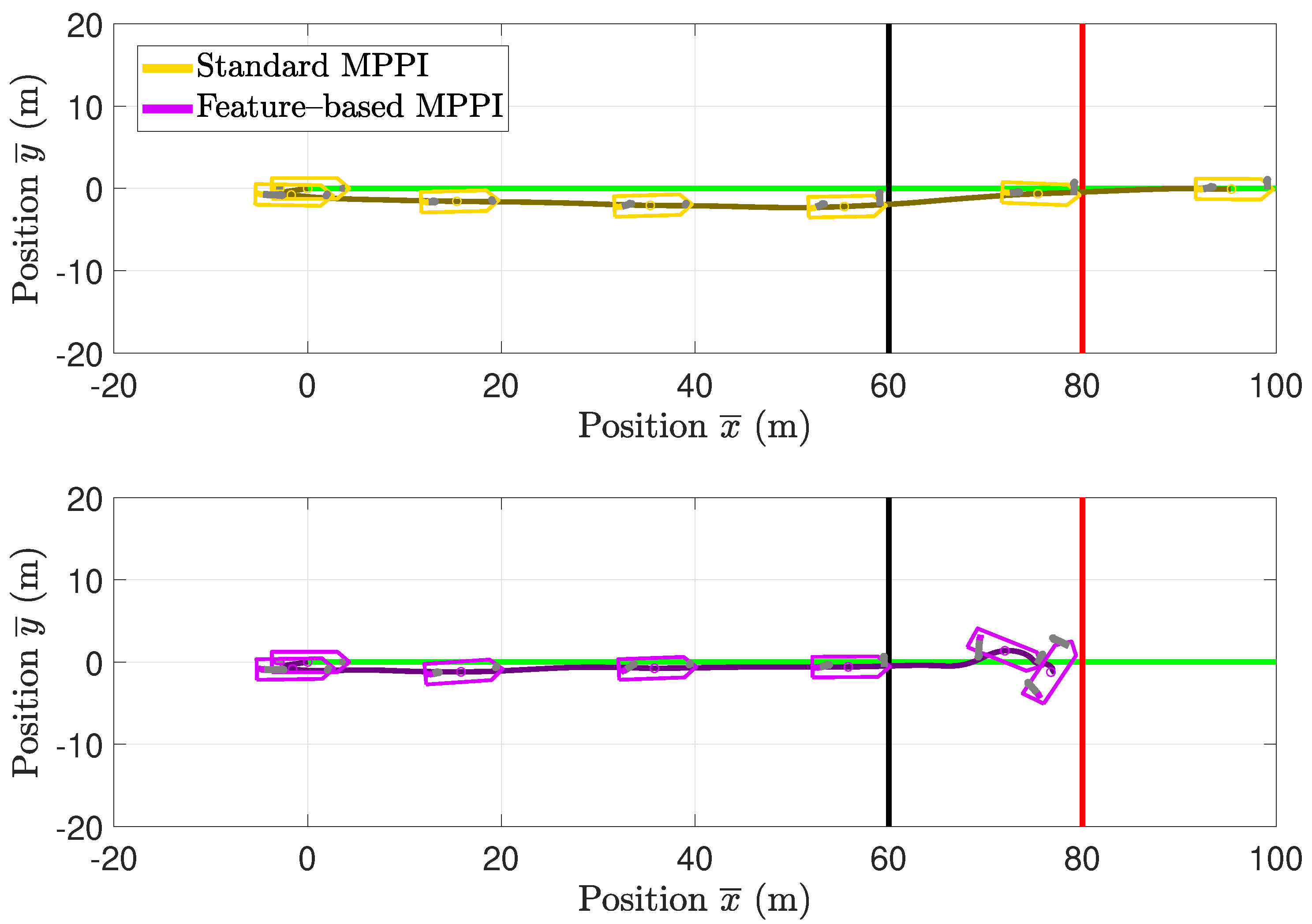
The MPPI controller presented in Section 2 and its feature-based extension introduced in Section 3 are embedded in a simulation environment to compare their performances when controlling the vessel model in the maritime application scenario described in Section 4. Therefore, the parameters derived in Section 5 are used. The vessel model including the actuator dynamics, the UKF according to [33], the MPPI controller and the feature-based MPPI controller are implemented in a simulation environment. According to [33], a constant river current is assumed with a velocity of 0.45 m/s and an orientation of 200 to the -axis. The simulation time is determined to 60 s. To compare the vessel’s behavior, both the standard MPPI approach and subsequently the feature-based MPPI approach are used to control the vessel. The resulting trajectories are compared in Figure 5. Furthermore, to visualize the orientation of the vessel along the trajectory, the vessel’s contour is plotted at the time instances with and s.
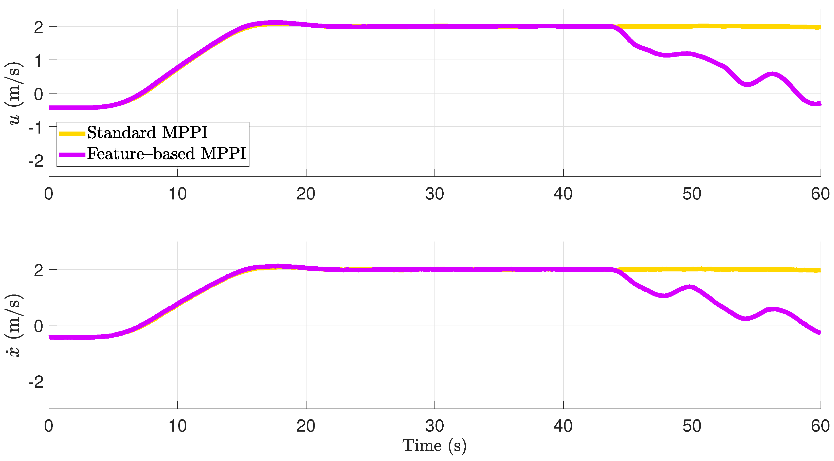
In the absence of an obstacle, both trajectories are quite similar in orientation and position. Note the position difference in occurs since it is only penalized slightly in (1a). After the obstacle appears, the different control approaches cause different behavior. While the system controlled by the standard MPPI controller causes a collision with the obstacle, the feature-based MPPI control approach can prevent this collision by performing a braking maneuver. The time courses of the body-fixed surge velocity and the vessel’s velocity in the direction of the -axis are shown in Figure 6. In the absence of the obstacle for 44 s, the plotted velocity components show the same behavior. After a learning phase of about 5 s immediately after activating the controllers, the vessel accelerates till it reaches the desired surge velocity. After the acceleration phase, the surge velocity is kept exact at 2 m/s. For 44 s using the feature-based approach, the vessel decelerates and reaches m/s at s. A comparison of the desired and the actual actuator values is given in Figure 7. Furthermore, in Figure 8, the caused costs using the different approaches are plotted over time. In contrast, using the standard MPPI controller, the vessel’s velocity does not change after the vessel appears. This effect results from the fact that, due to the small explored state-space using conventional MPPI control, all predicted trajectories cause a collision for 44 s.
Consequently, the vessel controlled by the standard MPPI approach collides with the obstacle at full speed at s. Regarding the input trajectories shown in Figure 7, the desired and actual actuator values are well fitting. Furthermore, in absence of an obstacle for 44 s, the input trajectories show nearly the same behavior. To keep the surge velocity at 2 m/s, the AT is driven with about 950 rpm after it reaches its maximal value during the acceleration phase. While the AT is used to reach and keep the desired velocity, the BT is used to compensate the disturbances due to the river current. Using the feature-based MPPI approach for s, the actuators’ trajectories lead to the braking behavior of the system.
To reach the maximal deceleration of the vessel, the AT’s orientation is inverted while its speed is maximized. Regarding the time series of the stage costs shown in Figure 8 in the absence of an obstacle for 44 s, both approaches cause the same costs. Both controllers find inputs leading to decreasing costs. After the obstacle is detected, the feature-based control approach applies the learned inputs corresponding to the defined feature. These inputs lead to increasing cost due to the decelerating surge velocity; however, in contrast to the standard MPPI approach, a collision is prevented and thus being in the high cost region of state-space is avoided. In this section, it was shown that, using the feature-based MPPI control approach, a significant improvement of the vessel behavior in a maritime application scenario is reached.
7. Full-Scale Results
To validate the simulation results, full-scale scale experiments are used. For this purpose, the algorithms used in the simulation will be transferred to the rapid prototyping systems of the research vessel Solgenia. A distributed structure of the components is used as already described in Section 5. In addition, the same controller parameters and cost functions are used as in the previous sections. The data are recorded directly during the experiments on the vessel. Regarding the disturbances immediately before the experiments, a river current of 0.46 m/s was determined in the vicinity of the trajectory. This current has an orientation of about and is thus almost opposite to the movement of the vessel on the trajectory. However, it should be noted that, although the current values were measured by allowing the research vessel to drift uncontrolled in the vicinity of the trajectory, they vary along the river and can therefore only be regarded as rough estimates, which, in reality, are overlaid by a stochastic component. In the experimental phase, the task described in Section 4 was executed once with a standard MPPI controller and once with a feature-based MPPI controller. For this purpose, the vessel’s position is stabilized at the beginning of the trajectory using feedback linearization according to [33] until the MPPI controller is activated. Then, the MPPI controller is activated for 60 s because both a collision or a collision avoidance maneuver could occur within this time span. In Figure 9, a comparison of the vessel’s behavior is shown for both experiments. In this figure, the vessel’s trajectories are plotted in local coordinates. Furthermore, the vessel’s contour and thus its orientation are shown at the time instances , with and s. While using the standard MPPI control visualized in the upper plot of Figure 9, the vessel collides with the obstacle; using feature-based MPPI control, a collision can be prevented. Compared to the simulation results presented in the previous section, in the full-scale experiments, the vessel tracks the reference trajectory with higher errors. This behavior is to be expected due to model inaccuracies and the disturbance vector assumed to be constant within the prediction horizon.
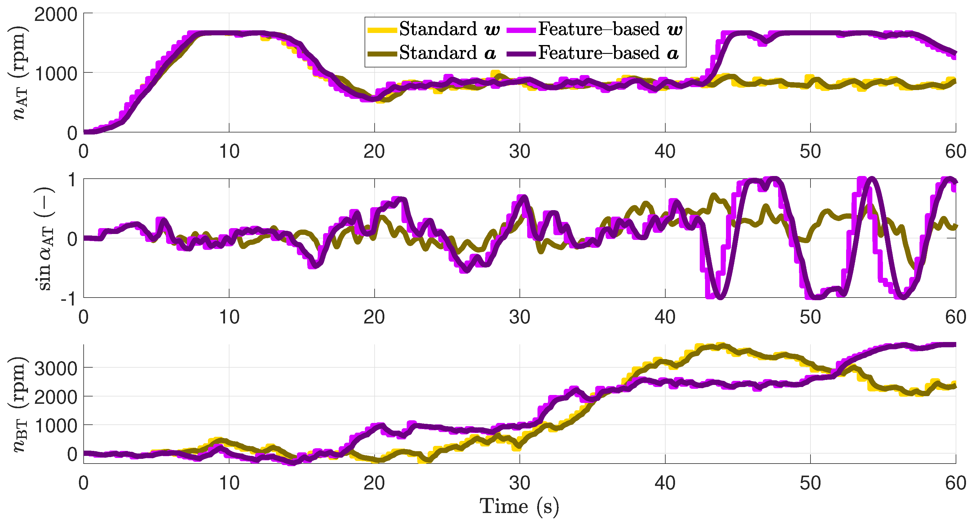
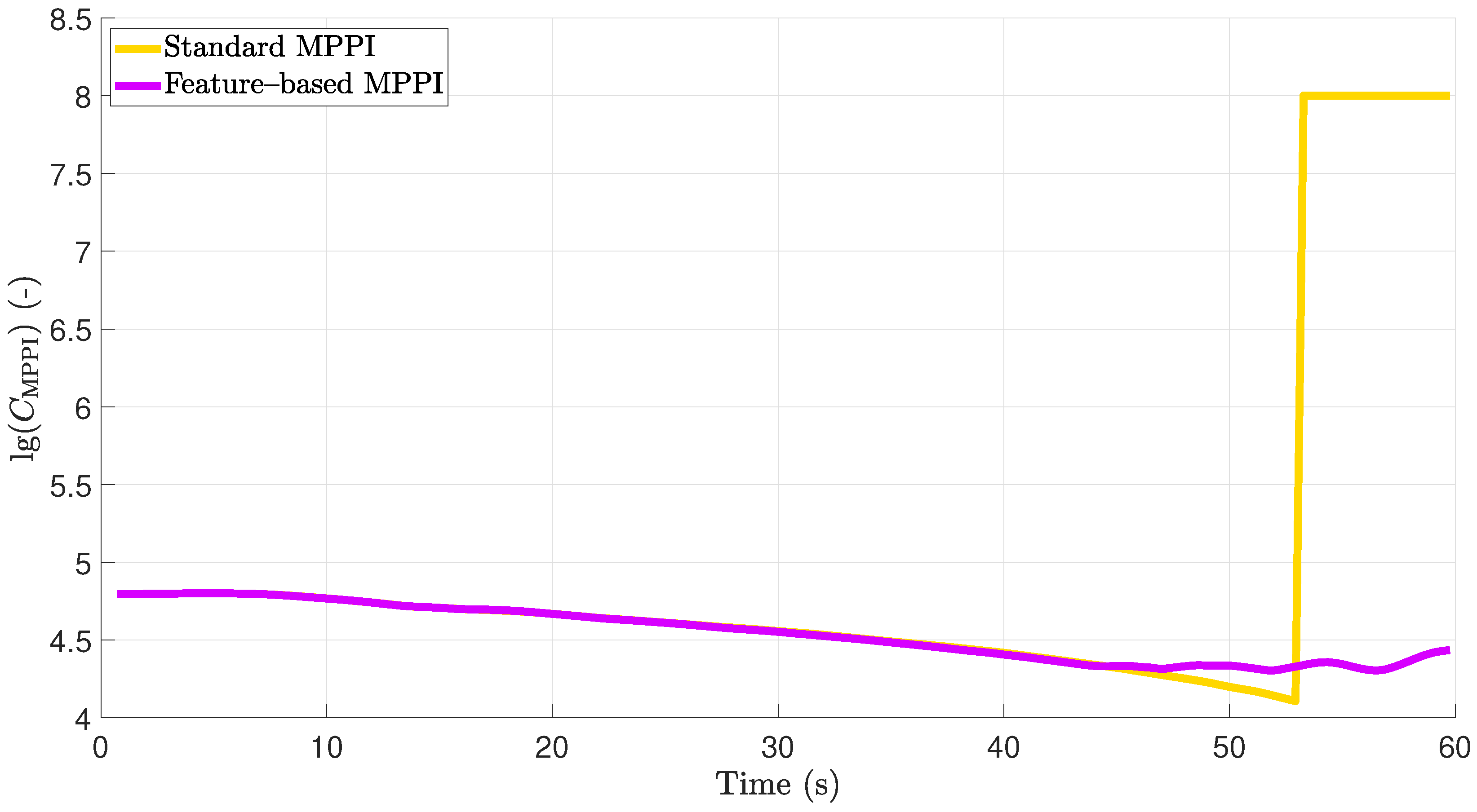
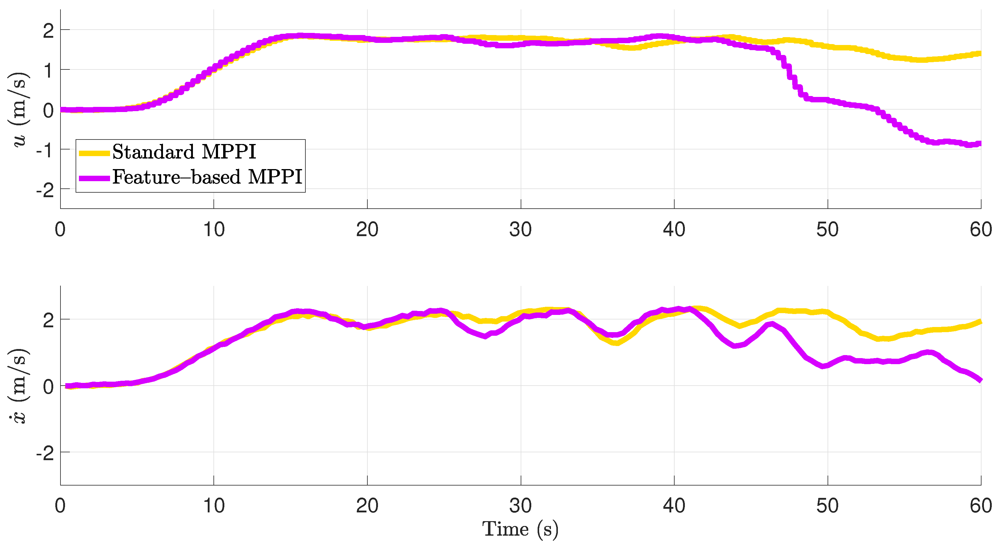
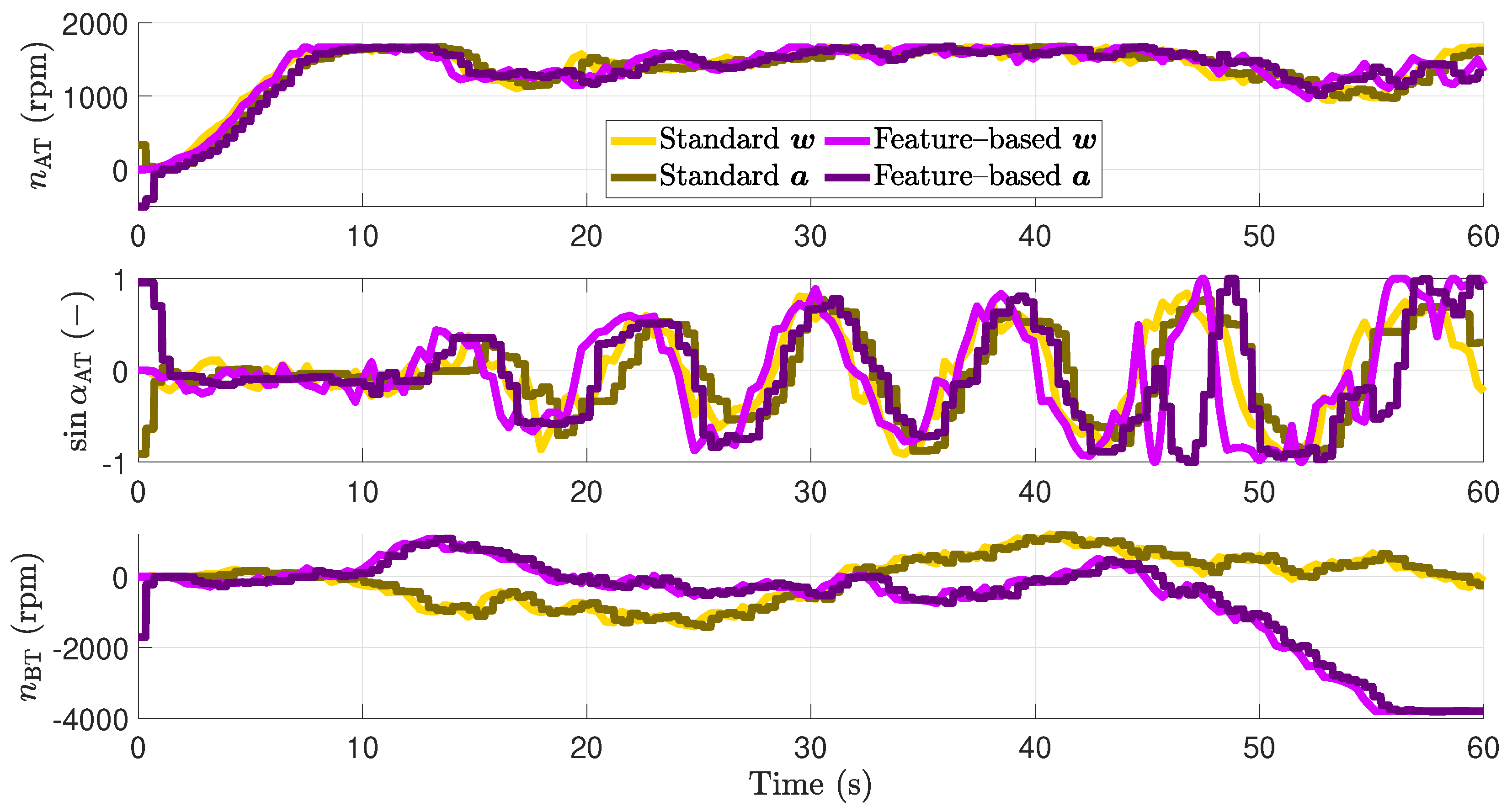
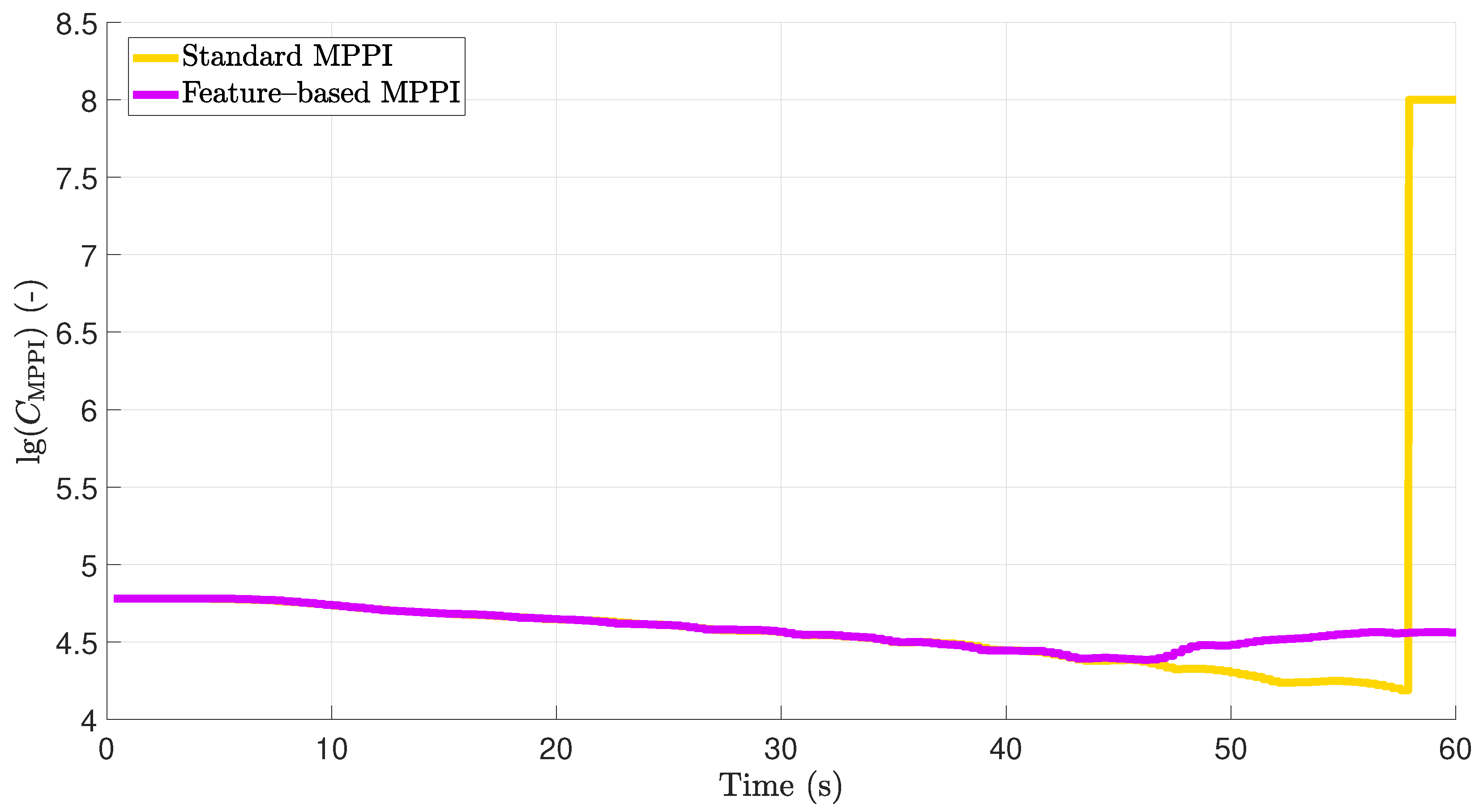
In the application example described, special focus is placed on the surge velocity component, since it is the most weighted in the selection of the coefficients of the cost function and thus the most important property in the case of the absence of an obstacle. However, if an obstacle is detected in this scenario, it is interesting to see how the speed develops in the direction of this obstacle. Thus, the surge velocity in body-fixed frame denoted by u and the velocity in direction of the obstacle denoted by are shown in Figure 10. The corresponding actuators’ signals are shown in Figure 11. The minimal path costs are plotted over time in Figure 12 in logarithmic scale. Using the described subordinated actuator control loops, the actual values of the actuators follow the desired values pretty good. Both the conventional MPPI controlled system and the feature-based MPPI controlled system show almost the same behavior for 44.6 s in the absence of an obstacle.
Standalone paragraphs require initial indentation, i change to indentation, please confirm At 5.1 s, the surge velocity increases until a maximum is reached with m/s at 15.5 s. After that, the surge velocity is kept at about 1.9 m/s by both controllers. It should be noted that both controllers achieve a good response to the disturbances. The difference between the desired and actual surge velocity is assumed to be due to the limitation of the propeller speed of the AT and model inaccuracies in this state region of high speed. At 44.6 s, the vessel collides with the obstacle within the prediction horizon. The standard MPPI controller does not decelerate after the detection of the obstacle. This effect results from the fact that, due to the small explored state-space using conventional MPPI control, all predicted trajectories cause a collision for 51.2 s. Consequently, predicted trajectories with surge velocity close to cause lower costs. In contrast, the feature-based MPPI controlled system explores more important areas of the state-space shown in Figure 1.
This allows the feature-based MPPI controller to apply the learned braking trajectory, which is optimal regarding the emergency braking feature (38), as soon as the obstacle is detected. Thus, it can also react excellently for 44.6 s and brake in time to avoid a collision. As can be seen in Figure 9, braking is achieved by counterclockwise rotation of the vessel, which allows the hydrodynamic effects of the vessel to be utilized in addition to the thruster forces of the propellers. As a consequence, while using the standard MPPI controller, the vessel’s velocity in the direction of the obstacle is 1.85 m/s at the moment hitting the obstacle; using the feature-based MPPI approach, the feature-based MPPI controller decelerates the velocity in the direction of the obstacle down to 0.05 m/s and thus avoids a collision. The minimum path costs, which are shown in Figure 12, are equal due to the equivalent system behavior of the two control approaches up to the detection of the obstacle. Using the standard MPPI approach after the detection, a low-cost region of state-space next to is explored. However, this leads to the fact that, already for 51 s, all predicted trajectories cause a collision. In contrast, using feature-based MPPI control, directly after the obstacle detection, the explored state-space is located at a region around the braking trajectory. This yields to higher costs, but even prevent the real high state-dependent costs caused by a collision. Using an MPC approach, the consideration of costs directly provides a quantitative quality criterion. Thus, if the cost curves in Figure 8 and Figure 12 are compared, it can be seen that the quality with regard to the cost function to be minimized is almost identical. In this section, it was shown that feature-based MPPI control in full-scale conditions can greatly expand and improve the behavior of a vessel and prevent collision without increasing the computational cost.
8. Conclusions
In this paper, an extension of the MPPI algorithm [4] is presented improving the sample efficiency by a knowledge-based feature definition. This is the first possibility to incorporate information subject to a scenario additive to the usual cost function into the control algorithm. The conventional MPPI and the presented feature-based MPPI control approaches are compared in a collision avoidance scenario. Therefore, a stochastic nonlinear OCP for enabling a vessel to follow a track and avoid collisions is presented and subsequently solved with both approaches. The performances of the algorithms are evaluated using data out of a simulation environment and full-scale experiments. In both simulation and full-scale experiments, while the standard MPPI would collide with an obstacle, the feature-based MPPI can prevent the collision although the same number of trajectories were drawn in both cases. In the absence of an obstacle, the feature-based MPPI controller learns an optimal braking trajectory that minimizes the feature costs subject to the modeled system dynamics. When the obstacle is detected, this is then successfully applied to avoid a collision. Thus, by inserting an emergency braking feature, the performance and usability of the algorithm could be increased significantly. Concerning other NMPC approaches, the MPPI control algorithm is characterized by a very good parallelization capability, since the samples can be drawn in different kernels. This property is not affected by the presented feature-based extension. Thus, the number of features that could be explored and learned can be increased by adding further parallel computing power. In future work, an evaluation of how the presented feature-based approach can be used in other sample-based NMPC algorithms could be scientifically valuable.
Author Contributions
Conceptualization, H.H., S.W. and J.R.; methodology, H.H.; software, H.H. and S.W.; validation, H.H. and S.W.; formal analysis, H.H.; investigation, H.H.; resources, J.R. and S.W.; data curation, H.H. and S.W.; writing—original draft preparation, H.H.; writing—review and editing, H.H., S.W., M.D. and J.R.; visualization, H.H.; supervision, S.W., M.D. and J.R.; project administration, J.R. All authors have read and agreed to the published version of the manuscript.
Funding
The article processing charge was funded by the Baden-Württemberg Ministry of Science, Research and Culture and the HTWG Konstanz—University of Applied Sciences in the funding programme Open Access Publishing.
Institutional Review Board Statement
Not applicable.
Data Availability Statement
The recorded data from simulations and real experiments, which are presented in this paper, can be downloaded using the link https://www.htwg-konstanz.de/fileadmin/pub/ou/isd/Regelungstechnik/Regelungstechnik_Data/MDPI_Machines22_Feature_Based_MPPI_Data_Simulation_and_Experiment.zip. Accessed on 23 May 2022.
Conflicts of Interest
The authors declare no conflict of interest.
Abbreviations
The following abbreviations are used in this manuscript:
| AWGN | Additive white Gaussian noise |
| CG | Center of gravity |
| HJB | Hamilton–Jacobi–Bellman |
| MABX | MicroAutoBox |
| MPPI | Model predictive path integral |
| NMPC | Nonlinear model predictive control |
| OCP | Optimal control problem |
| RL | Reinforcement learning |
| UKF | Unscented Kalman filter |
References
- Homburger, H.; Wirtensohn, S.; Reuter, J. Feature-Based Proposal Density Optimization for Nonlinear Model Predictive Path Integral Control. In Proceedings of the 6th IEEE Conference on Control Technology and Applications (CCTA), Trieste, Italy, 22–25 August 2022. [Google Scholar]
- Kleinert, H. Path Integrals in Quantum Mechanics, Statistics, Polymer Physics, and Financial Markets, 5th ed.; World Scientific Publishing Ltd.: Singapore, 2009. [Google Scholar]
- Kappen, H.J. Path Integrals and Symmetry Breaking for Optimal Control Theory. J. Stat. Mech. Theory Exp. 2005, 2005, P11011. [Google Scholar] [CrossRef] [Green Version]
- Williams, G.; Wagener, N.; Goldfain, B.; Drews, P.; Rehg, J.; Boots, B.; Theodorou, E. Information Theoretic MPC for Model-Based Reinforcement Learning. In Proceedings of the IEEE International Conference on Robotics and Automation (ICRA), Singapore, 29 May 2017–3 June 2017. [Google Scholar]
- Schaal, S.; Atkeson, C. Learning Control in Robotics. IEEE Robot. Autom. Mag. 2010, 10, 20–29. [Google Scholar] [CrossRef]
- Theodorou, E.A.; Buchli, J.; Schaal, S. A Generalized Path Integral Control Approach to Reinforcement Learning. J. Mach. Learn. Res. 2010, 11, 3137–3181. [Google Scholar]
- Kappen, H.J.; Ruiz, H. Adaptive Importance Sampling for Control and Inference. J. Stat. Phys. 2016, 162, 1244–1266. [Google Scholar] [CrossRef] [Green Version]
- Gómez, V.; Thijssen, S.; Symington, A.; Hailes, S.; Kappen, H.J. Real-Time Stochastic Optimal Control for Multi-agent Quadrotor Systems. In Proceedings of the 26th International Conference on Automated Planning and Scheduling (ICAPS 16), London, UK, 12–17 June 2016; 2015. [Google Scholar]
- Homburger, H.; Wirtensohn, S.; Reuter, J. Swinging Up and Stabilization Control of the Furuta Pendulum using Model Predictive Path Integral Control. In Proceedings of the 30th Mediterranean Conference on Control and Automation (MED), Athens, Greece, 28 June–1 July 2022. [Google Scholar]
- Theodorou, E.A.; Todorov, E. Relative entropy and free energy dualities: Connections to path integral and KL control. In Proceedings of the IEEE 51st Annual Conference on Decision and Control (CDC), Grand Wailea Maui, HI, USA, 10–13 December 2012; pp. 1466–1473. [Google Scholar]
- Theodorou, E.A. Nonlinear Stochastic Control and Information Theoretic Dualities: Connections, Interdependencies and Thermodynamic Interpretations. Entropy 2015, 17, 3352–3375. [Google Scholar] [CrossRef]
- Kappen, H.J. An Introduction to Stochastic Control Theory, Path Integrals and Reinforcement Learning. Coop. Behav. Neural Syst. Ninth Granada Lect. 2007, 887, 149–181. [Google Scholar]
- Thijssen, S.; Kappen, H.J. Path Integral Control and State Dependent Feedback. Phys. Rev. E 2015, 91, 032104. [Google Scholar] [CrossRef] [PubMed] [Green Version]
- Gandhi, M.S.; Vlahov, B.; Gibson, J.; Williams, G.; Theodorou, E. Robust Model Predictive Path Integral Control: Analysis and Performance Guarantees. IEEE Robot. Autom. Lett. 2021, 6, 1423–1430. [Google Scholar] [CrossRef]
- Yin, J.; Zhang, Z.; Theodorou, E.; Tsiotras, P. Improving Model Predictive Path Integral using Covariance Steering. arXiv 2021, arXiv:2109.12147. [Google Scholar]
- Kusumoto, R.; Palmieri, L.; Spies, M.; Csiszar, A.; Arras, K.O. Informed Information Theoretic Model Predictive Control. In Proceedings of the International Conference on Robotics and Automation (ICRA), Montreal, Canada, 20–24 May 2019; pp. 2047–2053. [Google Scholar]
- Williams, G.; Drews, P.; Goldfain, B.; Rehg, J.M.; Theodorou, E. Information-Theoretic Model Predictive Control: Theory and Applications to Autonomous Driving. IEEE Trans. Robot. 2018, 34, 1603–1622. [Google Scholar] [CrossRef] [Green Version]
- Abdelaal, M.; Hahn, A. NMPC-based trajectory tracking and collision avoidance of unmanned surface vessels with rule-based colregs confinement. In Proceedings of the IEEE Conference on Systems, Process and Control (ICSPC), Hammamet, Tunisia, 16–18 December 2016; pp. 23–28. [Google Scholar]
- Lutz, M.; Meurer, T. Optimal trajectory planning and model predictive control of underactuated marine surface vessels using a flatness-based approach. arXiv 2021, arXiv:2101.12730. [Google Scholar]
- Bärlund, A.; Linder, J.; Feyzmahdavian, H.R.; Lundh, M.; Tervo, K. Nonlinear MPC for combined motion control and thrust allocation of ships. In Proceedings of the 21st IFAC Wolrd Congress, Berlin, Germany, 11–17 July 2020. [Google Scholar]
- Zare, N.; Brandoli, B.; Sarvmaili, M.; Soares, A.; Matwin, S. Continuous Control with Deep Reinforcement Learning for Autonomous Vessels. arXiv 2021, arXiv:2106.14130. [Google Scholar]
- Martinsen, A.; Lekkas, A. Curved Path Following with Deep Reinforcement Learning: Results from Three Vessel Models. In Proceedings of the IEEE Oceans MTS, Charleston, SC, USA, 22–25 October 2018; pp. 1–8. [Google Scholar]
- Yin, Z.; He, W.; Yang, C.; Sun, C. Control Design of a Marine Vessel System Using Reinforcement Learning. Neurocomputing 2018, 311, 353–362. [Google Scholar] [CrossRef] [Green Version]
- Homburger, H.; Wirtensohn, S.; Reuter, J. Docking Control of a Fully-Actuated Autonomous Vessel using Model Predicitve Path Integral Control. In Proceedings of the 20th European Control Conference (ECC), London, UK, 12–15 July 2022. [Google Scholar]
- Lloyd. Articles of the Convention on the International Regulations for Preventing Collisions at Sea, 1972; Lloyd’s Register of International Maritime Organization: London, UK, 2005. [Google Scholar]
- Kinjo, L.M.; Wirtensohn, S.; Reuter, J.; Menard, T.; Gehan, O. Trajectory tracking of a fully-actuated surface vessel using nonlinear model predictive control. In Proceedings of the 13th IFAC Conference on Control Applications in Marine Systems, Robotics, and Vehicles (CAMS), Oldenburg, Germany, 22–24 September 2021; pp. 51–56. [Google Scholar]
- Fossen, T.I. Marine Control Systems: Guidance, Navigation and Control of Ships, Rigs and Underwater Vehicles, 1st ed.; Marine Cybernetics: Trondheim, Norway, 2002. [Google Scholar]
- Blanke, M. Ship Propulsion Losses Related to Automatic Steering and Prime Mover Control, 1st ed.; Technical University of Denmark: Lyngby, Denmark, 1981. [Google Scholar]
- Ramachandran, D.; Amir, E. Bayesian Inverse Reinforcement Learning. In Proceedings of the 20th International Joint Conference on Artificial Intelligence, Hyderabad, India, 6–12 January 2007. [Google Scholar]
- Ng, A.Y.; Russell, S. Algorithms for Inverse Reinforcement Learning. In Proceedings of the 17th International Conference on Machine Learning (ICML), San Francisco, CA, USA, 29 June–2 July 2000. [Google Scholar]
- Arora, S.; Doshi, P. A Survey of Inverse Reinforcement Learning: Challenges, Methods and Progress. Artif. Intell. 2021, 297, 103500. [Google Scholar] [CrossRef]
- Google Maps. Rhine River. Available online: https://www.google.com/maps/@47.6679863,9.1762762,16.96z (accessed on 5 May 2022).
- Wirtensohn, S.; Hamburger, O.; Homburger, H.; Kinjo, L.M.; Reuter, J. Comparison of Advanced Control Strategies for Automated Docking. In Proceedings of the 13th IFAC Conference on Control Applications in Marine Systems, Robotics, and Vehicles (CAMS), Oldenburg, Germany, 22–24 September 2021; pp. 295–300. [Google Scholar]
Figure 1.
Explored state–space in a full–scale experiment visualized by sampled trajectories using proposal densities with mean (red) and mean (blue) representing the emergency braking feature. The actuators’ force vectors are drawn in red. The desired trajectory is visualized in green.
Figure 1.
Explored state–space in a full–scale experiment visualized by sampled trajectories using proposal densities with mean (red) and mean (blue) representing the emergency braking feature. The actuators’ force vectors are drawn in red. The desired trajectory is visualized in green.

Figure 2.
Photography and technical drawing of the research vessel Solgenia. (a) photography of the research vessel Solgenia on Lake Constance in front of the Constance harbor; (b) technical drawing of the research vessel Solgenia with local and body-fixed coordinate systems, geometrical parameters and thruster forces.

Figure 3.
Bird’s eye view on the Rhine river between the docking area and the open lake [32]. The locations of and are specified in Table 3. The desired path is drawn in green. The borders to the inadmissible area next to the river bank are visualized in red. Due to the application scenario, the width and orientation of the river are approximated by = 120 m and = −31.96 .

Figure 4.
Distributed and modularized control architecture for full-scale experiments on research vessel Solgenia. The connections are realized via UDP and CAN protocol.
Figure 4.
Distributed and modularized control architecture for full-scale experiments on research vessel Solgenia. The connections are realized via UDP and CAN protocol.

Figure 5.
Comparison of the resulting trajectories of the vessel in the simulation environment. While the upper plot shows the performance of standard MPPI control, the lower plot shows the performance of the feature–based MPPI control approach. Both plots use transformed coordinates calculated by (30). The green lines visualize the reference trajectories in both plots. After passing the black line, the vessel detects the obstacle visualized as a red line.

Figure 6.
Comparison of the body–fixed surge velocity u and the velocity in simulation.

Figure 7.
Comparison of the resulting input trajectories of the vessel in the simulation environment.
Figure 7.
Comparison of the resulting input trajectories of the vessel in the simulation environment.

Figure 8.
Comparison of costs in the simulation scenarios plotted over time. Note the logarithmic representation of the plotted costs.
Figure 8.
Comparison of costs in the simulation scenarios plotted over time. Note the logarithmic representation of the plotted costs.

Figure 9.
Comparison of the resulting trajectories of the vessel in full–scale experiments at Rhine river in Constance. Both plots use transformed coordinates calculated by (30). The green lines visualize the reference trajectories in both plots. After passing the black line, the vessel detects the obstacle visualized as a red line.

Figure 10.
Comparison of the body–fixed surge velocity u and the velocity in direction in local frame.
Figure 10.
Comparison of the body–fixed surge velocity u and the velocity in direction in local frame.

Figure 11.
Comparison of the resulting input trajectories of the vessel in the full–scale experiments.
Figure 11.
Comparison of the resulting input trajectories of the vessel in the full–scale experiments.

Figure 12.
Comparison of costs plotted over time in full-scale experiments. Note the logarithmic representation of the cost.
Figure 12.
Comparison of costs plotted over time in full-scale experiments. Note the logarithmic representation of the cost.


Table 1.
Identified vessel parameters of the dynamic model [26] and the parameters of the actuators’ models [24].
| Vessel’s Dynamics Parameter | Value | Actuators’ Dynamics Parameter | Value |
|---|---|---|---|
| m | 3100 kg | 2300 rpm | |
| 0 m | 105 ms | ||
| 21,179 kgm | 240 ms | ||
| kg | 71.66 1/s | ||
| kg | - | ||
| kgm | 95 ms | ||
| kgm | 160 ms | ||
| Ns/m | 1.496 rad/s | ||
| Ns/m | 3800 rpm | ||
| Ns/m | 270 ms | ||
| Ns/m | 80 ms | ||
| Ns/m | 10,000 1/s |
Table 2.
Identified parameters of the actuators’ thrust models according to [26].
Table 2.
Identified parameters of the actuators’ thrust models according to [26].
| Parameter | Value | Parameter | Value |
|---|---|---|---|
| 0.9047 | 0.21 | ||
| 0.6545 | 0.24 | ||
| 0.36 m | 1000 kg/m | ||
| 0.23 m | 2.9 m |
Table 3.
Significant points specifying the application scenario.
| Point | Latitude | Longitude | Description |
|---|---|---|---|
| P1 | 47.668279218023123 | 9.174018424704204 | Start position |
| P2 | 47.666282640256334 | 9.178596676673507 | End position |
Table 4.
Controller parameters of the standard MPPI and the feature-based MPPI approaches.
| Parameter | MPPI | Feature-Based MPPI |
|---|---|---|
| K | 9000 | 8500 |
| T | 41 | 41 |
| 1 | 1 | |
| Equation (33) | Equation (33) | |
| 0 | 0 | |
| - | 500 | |
| - | Equation (38) | |
| - | Equation (38) |
Table 5.
Coefficients of the costs (33) and the feature costs (38).
| Parameter | Value | Parameter | Value |
|---|---|---|---|
| 500 1/m | 409.9 m | ||
| 200 1/m | 2 m/s | ||
| 2500 1/rad | 300 s/m | ||
| 5000 s/m | 30 s/m | ||
| 10 s/m | 10 s/rad | ||
| 7500 s/rad | 60 m | ||
| 80 m |
Publisher’s Note: MDPI stays neutral with regard to jurisdictional claims in published maps and institutional affiliations. |
© 2022 by the authors. Licensee MDPI, Basel, Switzerland. This article is an open access article distributed under the terms and conditions of the Creative Commons Attribution (CC BY) license (https://creativecommons.org/licenses/by/4.0/).
Share and Cite
MDPI and ACS Style
Homburger, H.; Wirtensohn, S.; Diehl, M.; Reuter, J. Feature-Based MPPI Control with Applications to Maritime Systems. Machines 2022, 10, 900. https://doi.org/10.3390/machines10100900
AMA Style
Homburger H, Wirtensohn S, Diehl M, Reuter J. Feature-Based MPPI Control with Applications to Maritime Systems. Machines. 2022; 10(10):900. https://doi.org/10.3390/machines10100900
Chicago/Turabian StyleHomburger, Hannes, Stefan Wirtensohn, Moritz Diehl, and Johannes Reuter. 2022. "Feature-Based MPPI Control with Applications to Maritime Systems" Machines 10, no. 10: 900. https://doi.org/10.3390/machines10100900
Note that from the first issue of 2016, this journal uses article numbers instead of page numbers. See further details here.