A New Trajectory Tracking Control Method for Fully Electrically Driven Quadruped Robot

Abstract

To improve the accuracy of tracking the trunk center-of-mass (CoM) trajectory and foot-end trajectory in a fully electrically driven quadruped robot, an efficient and practical new trajectory tracking control method is designed. The proposed trajectory tracking method is mainly divided into trunk balance controller (TBC) and swing leg controller (SLC). In TBC, a quadruped robot dynamics model is developed to find the optimal foot-end force that follows the trunk CoM trajectory based on the model predictive control (MPC) principle. In SLC, the Bessel curve is planned as the desired trajectory at the foot-end, while the desired trajectory is tracked by a virtual spring-damping element driving the foot-end, meanwhile, the radial basis function neural network (RBFNN) is applied for supervisory control to improve the control performance for the system. The experimental results show that the control method can modify the robot’s foot-end trajectory tracking effect, so that the stability error can be eliminated and the robustness of the controller can be improved, meanwhile, the linear and circular trajectory for CoM can be tracked accurately and quickly.

1. Introduction

The quadruped robot has good terrain adaptability. It has broad application prospects in complex situations, such as disaster relief and rescue, planet exploration, military investigation and so on [1,2]. It can perform tasks that traditional wheeled robots and tracked robots cannot perform [3,4,5]. Quadruped robot control technology is mainly divided into task decision-making, environment perception, trajectory planning and trajectory tracking control [6]. Among them, efficient and stable trajectory tracking control technology is the prerequisite for quadruped robots to realize intelligence and practicality. However, the research on trajectory tracking technology is often concentrated in the field of unmanned vehicles, and there is relatively little research on trajectory tracking technology of quadruped robots.

Chen et al. [7] measured the position and direction of the robot’s body in real time based on the state information feedback by the motor and the kinematics model to calculate the robot’s trajectory and carried out the research on the trajectory tracking control of the quadruped robot based on the closed-loop control strategy. The strategy is too simple, and its reliability and effectiveness are difficult to apply to quadruped robots under high-speed motion. Oliveira et al. [8] proposed a control strategy for electric drive quadruped robots and developed a trajectory tracking motion control algorithm based on PID control. However, due to the control delay of PID, it could not provide good tracking performance. Chen et al. [9] applied an adaptive fuzzy algorithm based on the PID algorithm to adjust the PID parameters to be applied in the leg joint control of the hydraulic quadruped robot to improve the tracking effect of the foot trajectory. This algorithm has a greater improvement than conventional PID in reducing the adjustment time and suppressing interference, but it has greater problems with the stability of the complex environment and the robot at high speed. In addition, the selection of the initial value of the fuzzy algorithm will greatly affect the tracking performance of the system.

Pratt et al. [10] first proposed virtual model control and applied it to biped robots. The VMC method uses imaginary virtual spring elements to connect the robot’s internal action points, or to connect the action points to the external environment, in order to generate the corresponding virtual forces to drive the robot to achieve the desired motion [11,12]. The HyQ robot developed by the Italian Institute of technology uses the virtual model of the leg to achieve better interaction with the ground [13,14]. Zhang et al. [15,16] proposed a trajectory tracking control method for quadruped robot diagonal trot gait based on a virtual model. This method sets up the support phase virtual model control and swing phase virtual model control, but only the static analysis of the system is carried out without considering the dynamics of the robot, which greatly simplifies the complexity of the model and leads to large errors in tracking control. In addition, the essence of the virtual model control method used is to construct a PD controller, a direct method based on intuitive control, which is fast and does not require complex calculations but does not promise accurate control [17].

As a common control method for biped robots, the Zero Moment Point (ZMP) based algorithm is also introduced into the gait control of quadruped robot trot. Kurazemu et al. [18] proposed a three-dimensional swing curve of the torso based on the ZMP method and controlled the Titan-VIII robot to achieve stable diagonal trot track tracking. SI et al. [19] used the ZMP stability criterion to plan the foot trajectory and realized the trajectory tracking of the trotting gait of the robot in the true-proof environment and the physical environment, respectively. However, the ZMP method is more suitable for the static gait control of the quadruped robot, and it is difficult to apply the ZMP stability criterion when a dynamic gait, such as the trot is adopted.

As a popular feedback control algorithm, MPC is widely used in industrial production control processes [20]. The MPC algorithm is a control method that considers the inputs, outputs and future states of the system and compares them with future reference signals when calculating the optimal control inputs of the system. In view of the control signal delay phenomenon existing in the PID algorithm, the MPC algorithm can take this delay into account in the model, so as to avoid this problem [21]. Carlo et al. [22] and Bledt et al. [23] proposed a quadruped robot motion control method based on MPC theory to determine the ground reaction during quadruped robot walking, but they focused on trunk control and ignored the coupling effect of leg control on the whole quadruped robot control system, resulting in a large steady-state error of leg trajectory. Thus, the stability and trajectory tracking accuracy of the quadruped robot is affected.

In the past few decades, intelligent control technology represented by neural networks has been developed rapidly [24]. A large number of studies show that neural networks are good at dealing with function approximation and uncertainty problems and have made great progress in dealing with uncertain nonlinear systems in continuous time [25]. Hwangbo et al. [26] adopted a deep reinforcement learning method and made the AnYmal robot faster than before in simulation. Chen et al. [27] proposed a reinforcement learning method based on the Actor-Critic to realize the disruption recovery of quadruped robots. Ma [28] used the Hopf oscillator to construct two central pattern generators (CPG) control networks, which were analyzed and modeled for their structures and controlled each joint of the quadruped robot according to the control signal output from the CPG network to achieve fast gait planning. However, this algorithm is too complex and slow in convergence, so it is difficult to be applied in practical engineering.

Through the above analysis, it can be found that most researchers have the following deficiencies in the path tracking of quadruped robots:

(1)

The trajectory tracking controller of a quadruped robot is often analyzed on the basis of a kinematic model, and the dynamic characteristics are not studied. Therefore, the accuracy of trajectory tracking is difficult to be further improved.

(2)

Trajectory tracking often adopts a simple closed-loop control strategy, which is difficult to be further popularized for quadruped robots with underactuated, multi-variable, strong coupling and nonlinear characteristics.

(3)

A large number of scholars have carried out research on the trajectory tracking control of quadruped robots, often focusing on the trajectory tracking of the robot trunk centroid, ignoring the impact of the accuracy of the quadruped robot leg trajectory tracking control on the overall control of the robot.

(4)

The MPC algorithm is an effective method to solve the trajectory tracking problem of unmanned vehicles, but whether it can meet the real-time performance requirements of quadruped robot trajectory tracking control needs to be further verified.

Aiming at the control problems mentioned in the trajectory tracking process of quadruped robots, a new control method for improving the trajectory tracking accuracy of quadruped robots is proposed. The trajectory tracking control algorithm is mainly divided into two parts: trunk balance controller [29,30] and swing leg trajectory tracking controller, the contributions of this work are organized as follows:

(1)

In the TBC, the trunk dynamic model of the quadruped robot is established and based on this model, a trajectory tracking method based on model predictive control theory is designed. Firstly, the dynamic model is discretized to obtain the state space equation. Secondly, the optimization objective function and constraints are established, and the solution of the future control quantity is transformed into the optimal solution of quadratic programming. Finally, the optimal solution is applied to the system.

(2)

In the SLC, a virtual model control method based on radial basis function neural networks (RBFNN) is designed. This control method uses the imaginary components to connect internal and external points, in order to generate virtual force to drive the foot-end to track the desired trajectory of the robot; at the same time, a supervise controller was designed based on RBFNN and online learning, optimizing the supervision of learning parameters of the controller, by weighting function to coordinate the two foot-end power output of the controller. The function of the two controllers is to ensure that the quadruped robot has good response characteristics while reducing the deviation during trajectory tracking by tracking the desired trajectory.

The balance controller and swing leg controller are switched by a finite state machine (FSM). The effectiveness of the proposed algorithm is verified by trajectory tracking test on a quadruped robot.

The remaining sections are outlined as follows. Section 2 introduces the leg kinematics and trunk dynamics model for quadruped robots. In Section 3, the trajectory tracking controller for the quadruped robot is designed, which mainly includes a leg controller and trunk balance controller. In Section 4, experiments are carried out to verify the effectiveness of the designed controller. Finally, the conclusion of this paper is given in Section 5.

2. Mathematical Model

2.1. Leg Kinematic Model

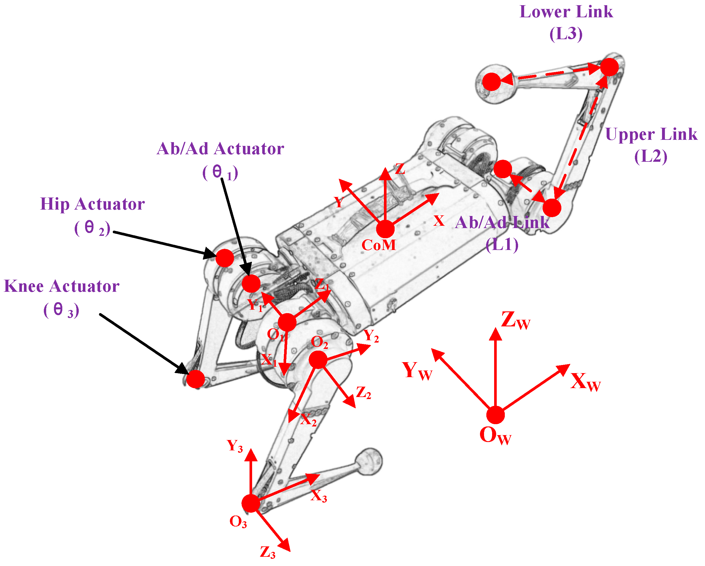
The motion of the quadruped robot is the relative motion of the trunk to the ground, which is achieved by the relative motion between the foot-end and the ground. The trunk and legs are considered as the base and open chain mechanisms, respectively, and the leg kinematics are modeled based on the D-H method [31,32]. The kinematic model for the legs of the quadruped robot is shown in Figure 1. The kinematic equation for the leg is (1).

$$\left[\begin{array}{c}{p}_x\\ p_y\\ p_z\end{array}\right]=\left[\begin{array}{c}{L}_3{s}_{2.3}+L_2{s}_2\\ L_1\ast \mathrm{Sign}\ast c_1+L_3\ast (s_1\ast c_{23})+L_2\ast c_2\ast s_1\\ L_1\ast \mathrm{Sign}\ast s_1-L_3\ast (c_1\ast c_{23})+L_2\ast c_1\ast c_2\end{array}\right]$$

(1)

where $\{\begin{array}{l}{s}_i=\sin {\theta }_i\\ c_i=\cos {\theta }_i\\ s_{ij}=\sin (i+j)\\ c_{ij}=\cos (i+j)\end{array}$ $i,j=1,2,3$. $\mathrm{Sign}=-1$ represents the right leg, $+1$ represents the left leg.

The position for the foot-end of the quadruped robot relative to the $O_1$ coordinate system can be expressed as $p=[p_x,p_y,p_z]$. The angle of the three joints at the leg is $\theta =\left[\begin{array}{ccc}{\theta }_1& {\theta }_2& {\theta }_3\end{array}\right]$. The leg Jacobian matrix is the partial differentiation from the position at the foot-end to the joint angle [33], that is $\frac{\delta \left(p_x,p_y,p_z\right)}{\delta ({\theta }_1,{\theta }_2,{\theta }_3)}$.

$$J=\left[\begin{array}{ccc}\frac{\partial p_x}{\partial {\theta }_1}& \frac{\partial p_y}{\partial {\theta }_1}& \frac{\partial p_z}{\partial {\theta }_1}\\ \frac{\partial p_x}{\partial {\theta }_2}& \frac{\partial p_y}{\partial {\theta }_2}& \frac{\partial p_z}{\partial {\theta }_2}\\ \frac{\partial p_x}{\partial {\theta }_3}& \frac{\partial p_y}{\partial {\theta }_3}& \frac{\partial p_z}{\partial {\theta }_3}\end{array}\right]=\left[\begin{array}{ccc}0& L_3\ast c_{23}+L_2\ast c_2& L_3\ast c_{23}\\ L_3\ast c_1\ast c_{23}+L_2\ast c_1\ast c_2-L_1\ast \mathrm{Sign}\ast s_1& -L_3\ast s_1\ast s_{23}-L_2\ast s_1\ast s_2& -L_3\ast s_1\ast s_{23}\\ L_3\ast s_1\ast c_{23}+L_2\ast c_2\ast s_1-L_1\ast \mathrm{Sign}\ast c_1& L_3\ast c_1\ast s_{23}+L_2\ast c_1\ast s_2& L_3\ast c_1\ast s_{23}\end{array}\right]$$

(2)

2.2. Dynamic Model

For the quadruped robot, the mass is concentrated in the geometric center of the trunk, while the leg is less than 10% of the overall mass. Therefore, it is reasonable to simplify the dynamic model without considering the legs [34,35]. Taking the attitude angle, centroid position, body angular velocity and centroid acceleration of the robot as state variables, in sum, the simplified dynamic model can be written in this form:

$$\mathsf{\Omega }=\left[\begin{array}{c}\mathsf{\Theta }\\ p\\ \omega \\ \ddot{p}\end{array}\right]$$

(3)

where $\mathsf{\Theta }=\left[\begin{array}{ccc}\phi & \theta & \psi \end{array}\right]$ are the roll, pitch and yaw angles of the robot system, which are the rotation angles of the CoM coordinate system around the $X_W$, $Y_W$ and $Z_W$ axis of the world coordinate system, respectively; $p$ is the position of the CoM; $\omega$ is the angular velocity in the world coordinates; $\ddot{p}$ is the centroid acceleration.

According to the Newton’s Second Law, the acceleration of the rigid body as:

$$\ddot{p}=\frac{{\displaystyle \sum _{i=1}^n{f}_i}}{m}-g$$

(4)

where $f_i\in R^3$ is the force acting on the contact patches, $r_i\in R^3$ is the vector from the CoM to the point of force, $g\in R^3$ is the acceleration of gravity, and $m$ is the mass of the robot. The rigid body dynamics in world coordinates are given by the following formula:

$$\frac{d}{dt}(I\omega )={\displaystyle \sum _{i=1}^n{r}_i\times f_i}$$

(5)

$$\dot{M}={\left[\omega \right]}_{\times }M$$

(6)

$$M=M_{Z_W}(\psi )M_{Y_W}(\theta )M_{X_W}(\phi )$$

(7)

where $I\in R^3$ is the inertia tensor in the world coordinate system, ${\left[\omega \right]}_{\times }\in R^{3\times 3}$ is defined as the skew-symmetric matrix, $M$ is the rotation matrix which transforms from body to world coordinates, $M_n(\alpha )$ represents a positive rotation of $\alpha$ about the n-axis.

In the dynamics model of a quadruped robot, the pitch angle and roll angle of the robot is approximated to 0, and the angular velocity dynamics of world coordinates can be approximated from the following formula:

$$\left[\begin{array}{c}\dot{\phi }\\ \dot{\theta }\\ \dot{\psi }\end{array}\right]\approx \left[\begin{array}{ccc}\cos (\psi )& \sin (\psi )& 0\\ -\sin (\psi )& \cos (\psi )& 0\\ 0& 0& 1\end{array}\right]\omega \approx M_{Z_W}{}^T(\psi )\omega$$

(8)

Through the above dynamic analysis, the dynamic state space equation for the quadruped robot system can be obtained. Rewriting the gravitational term into the state quantity for the system, then the robot dynamic state equation can be written as:

$$\frac{d}{dt}\left[\begin{array}{c}\widehat{\mathsf{\Theta }}\\ \widehat{p}\\ \widehat{\omega }\\ \begin{array}{l}\widehat{\dot{p}}\\ G\end{array}\end{array}\right]=\left[\begin{array}{ccccc}{O}_3& O_3& M_{Z_W}(\psi )& O_3& 0\\ O_3& O_3& O_3& 1_3& 0\\ O_3& O_3& O_3& O_3& 0\\ O_3& O_3& O_3& O_3& 1\\ 0& 0& 0& 0& 0\end{array}\right]\left[\begin{array}{c}\widehat{\mathsf{\Theta }}\\ \widehat{p}\\ \widehat{\omega }\\ \begin{array}{l}\widehat{\dot{p}}\\ G\end{array}\end{array}\right]+\left[\begin{array}{cccc}{O}_3& O_3& O_3& O_3\\ O_3& O_3& O_3& O_3\\ {\widehat{I}}^{-1}{[r_1]}_{\times }& {\widehat{I}}^{-1}{[r_2]}_{\times }& {\widehat{I}}^{-1}{[r_3]}_{\times }& {\widehat{I}}^{-1}{[r_4]}_{\times }\\ 1_3/m& 1_3/m& 1_3/m& 1_3/m\\ 0& 0& 0& 0\end{array}\right]\left[\begin{array}{c}{f}_1\\ f_2\\ f_3\\ f_4\end{array}\right]$$

(9)

3. Control Design

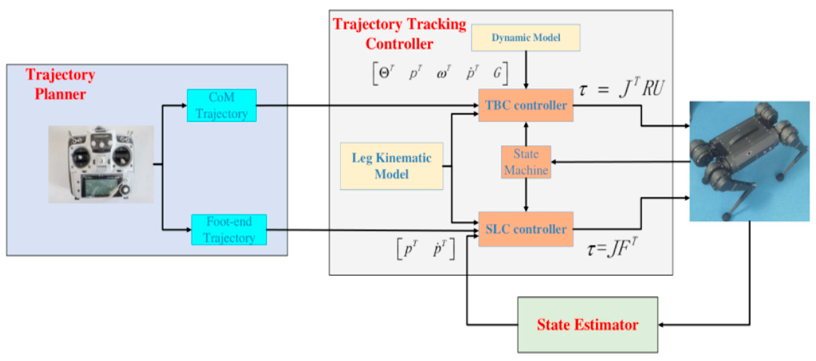
As shown in Figure 2, the whole motion controller for the quadruped robot consists of three parts, which are the trajectory planner, the trajectory tracking controller and the state estimator. The trajectory planner generates both the desired CoM trajectory and foot-end trajectory for the robot. In practical application, the desired trajectory of the CoM contains only the velocity and position of the $X_W$ and $Y_W$ axis in the world coordinate system, as well as the position, yaw and yaw rate of the $Z_W$ axis, and the other states are always set to 0. The Bezier curve is used for the expected trajectory for the foot-end. The trajectory tracker control consists of TBC, SLC and a finite state machine. TBC and SLC are the focus of this paper which are explained in detail in the following. The finite state machine uses an event-based gait switching. The state estimator is used to estimate the state information for the robot in real time by a fusion algorithm based on the two-level sensors. It first uses an inertial measurement unit to estimate orientation, while the second fuses accelerometers with leg kinematics to estimate position and velocity [36].

3.1. Foot-End Trajectory Planning

In order to minimize the impact when the robot’s foot-end touches the ground, the expected foot-end trajectory is generally planned as a cycloid. Bezier curves are widely used as foot-end trajectories for quadruped robots with advantages, such as simple control, high descriptive power and eased generation for complex smooth curves [37,38]. The Bezier curve can be expressed as follows:

$$q({\tau }_i)={{\displaystyle \sum _{k=0}^b(\begin{array}{c}b\\ k\end{array})P_k(1-{\tau }_i)}}^{b-k}{\tau }_i{}^k,{\tau }_i\in [0,1]$$

(10)

where $b$ is the order of the Bezier curve, $q({\tau }_i)$ is the interpolation point at ${\tau }_i$, and $P_k$ is the Kth control point. By taking the value of parameter ${\tau }_i$ in $[0,1]$, any interpolation point between $P_0$ and $P_k$ can be generated. In this paper, the third-order Bezier curve is used and its expression is:

$$q({\tau }_i)=(1-{\tau }_i{)}^3{P}_0+3{\tau }_i(1-{\tau }_i{)}^2{P}_1+3{\tau }_i{}^3(1-{\tau }_i)P_2+{\tau }_i{}^3{P}_3$$

(11)

3.2. Design of TBC

The TBC is used to control the stable movement of the quadruped robot trunk. According to the desired state quantities, such as trunk pose, height and velocity, the ground support force required by the robot is solved based on MPC [39], the output force at the foot-end is obtained from applied force and reaction force, and then the output torque of each joint on the legs is solved by the leg Jacobian matrix. Based on the state space dynamics model, the prediction equation and optimization solution for MPC are derived sequentially. The TBC architecture is shown in Figure 3.

3.2.1. Prediction Equation

The dynamic state space model for quadruped robots is:

$$\dot{x}(t)=A_c(\psi )x(t)+B_c(r_1,r_2,r_3,r_4,\psi )u(t)$$

(12)

where $A_c\in R^{13\times 13}$, $B_c\in R^{13\times 12}$.

In order to be able to apply this model to the design of the model predictive controller. The forward Euler discretization process is performed on the above equation of state [40]:

$$x(k+1)=A_{k}x(k)+B_{k}u(k)$$

(13)

where $x=\left[\begin{array}{ccccc}{\mathsf{\Theta }}^T& p^T& {\omega }^T& {\dot{p}}^T& G\end{array}\right]$,$u=\left[\begin{array}{cccc}{f}_1& f_2& f_3& f_4\end{array}\right]$,

$A_k=(I+TA)=\left[\begin{array}{ccccc}{1}_3& O_3& T\ast M_{Z_W}(\psi )& O_3& 0\\ O_3& 1_3& O_3& T\ast 1_3& 0\\ O_3& O_3& 1_3& O_3& 0\\ O_3& O_3& O_3& 1_3& T\\ 0& 0& 0& 0& 0\end{array}\right],$$B_k=TB=\left[\begin{array}{cccc}{O}_3& O_3& O_3& O_3\\ O_3& O_3& O_3& O_3\\ {\widehat{I}}^{-1}{[r_1]}_{\times }T& {\widehat{I}}^{-1}{[r_2]}_{\times }T& {\widehat{I}}^{-1}{[r_3]}_{\times }T& {\widehat{I}}^{-1}{[r_4]}_{\times }T\\ 1_3\ast T/m& 1_3\ast T/m& 1_3\ast T/m& 1_3\ast T/m\\ 0& 0& 0& 0\end{array}\right]$,

$T$ is the sampling time, then the state equation of the system in the next $h$ step:

$$\begin{array}{l}{x}_{k+1}=A{x}_k+B{U}_k\\ x_{k+2}=A{x}_{k+1}+B{U}_{k+1}=A(A{x}_k+B{U}_k)+B{U}_{k+1}\\ =A^2{x}_k+AB{U}_k+B{U}_{k+1}\\ x_{k+3}=A^3{x}_k+A^{2}B{U}_k+AB{U}_{k+1}+B{U}_{k+2}\\ ⋮\\ x_{k+h}=A^h{x}_k+A^{h-1}B{U}_k+\cdots +AB{U}_{k+1}+B{U}_{k+h-1}\end{array}$$

(14)

Then, the trajectory state equation for the system at $h$ steps in the future is

$$\overline{X}=A{x}_k+BU$$

(15)

where $\overline{X}={[x_{k+1}{x}_{k+2}\cdots x_{k+h}]}^T$, $U={[U_k{U}_{k+1}\cdots U_{k+h-1}]}^T$, $A={[A{A}^2\cdots A^h]}^T$, $B=\left[\begin{array}{ccccc}B& 0& 0& \cdots & 0\\ AB& B& 0& \cdots & 0\\ A^{2}B& AB& B& \cdots & 0\\ ⋮& ⋮& ⋮& ⋮& ⋮\\ A^{h-1}B& A^{h-2}B& A^{h-3}B& \cdots & B\end{array}\right]$

3.2.2. Optimization Solution

$U$ in the state equation is unknown, and the control quantity in the control time domain can be obtained only by setting a suitable optimization objective function [41]. The optimization objective function is shown in (16) below. By finding the current optimal input, the robot can accurately track the desired value while keeping the control input value as small as possible because the motor torque is limited in the actual robot motion.

$$L(x,f)=\underset{x,f}{\min }{\displaystyle \sum _{i=1}^{N_p}{\Vert x(i+1)-x_{ref}(i+1)\Vert }_Q^2+{\displaystyle \sum _{i=1}^{N_c-1}{\Vert u(i)\Vert }_V^2}}$$

(16)

The first term reflects the ability of the system to track the reference trajectory, and the second term is the requirement for the control quantity to change smoothly. $Q$ and $V$ are the weight matrices. $N_p$ is the control step size, $N_c$ is the prediction step size. The whole objective function is to enable the robot to track the desired trajectory quickly and smoothly.

This paper mainly considers the limit constraint of control quantity in the control process. The expression of control quantity is:

$$u_{\min }(t+k)\le u(t+k)\le u_{\max }(t+k)$$

(17)

where $k=0,1,2,\dots ,N_c-1$.

The optimization solution problem for the model predictive controller at each step is equated to the following quadratic programming problem [42]:

$$\underset{f}{{\displaystyle \min }}(\frac{1}{2}{U}^{T}HU+V^{T}U)$$

(18)

where $c_{\min }\le CU\le c_{\max }$, $H=2(B^{T}QB+V)$, $V=2B^{T}Q(x-x_{ref})$.

After solving the above formula in each control cycle, a series of control inputs in the control time domain can be obtained:

$$U=[U_k,U_{k+1},U_{k+2},\cdots ,U_{k+h-1}]$$

(19)

According to the MPC principle, the first control input in the control time domain is applied to the system, and then the output torque of each joint can be solved by transposing the leg Jacobi matrix. During the TBC operation, the joint torques are calculated as follows.

$${\tau }_i=J_i{}^T{M}_i{U}_i$$

(20)

In the new control cycle, the system re-predicts the state quantities in the next time domain based on the current state information and then goes through an optimization process to obtain a new sequence of control quantities. The cycle continues until the robot completes the control process.

3.3. Design of SLC

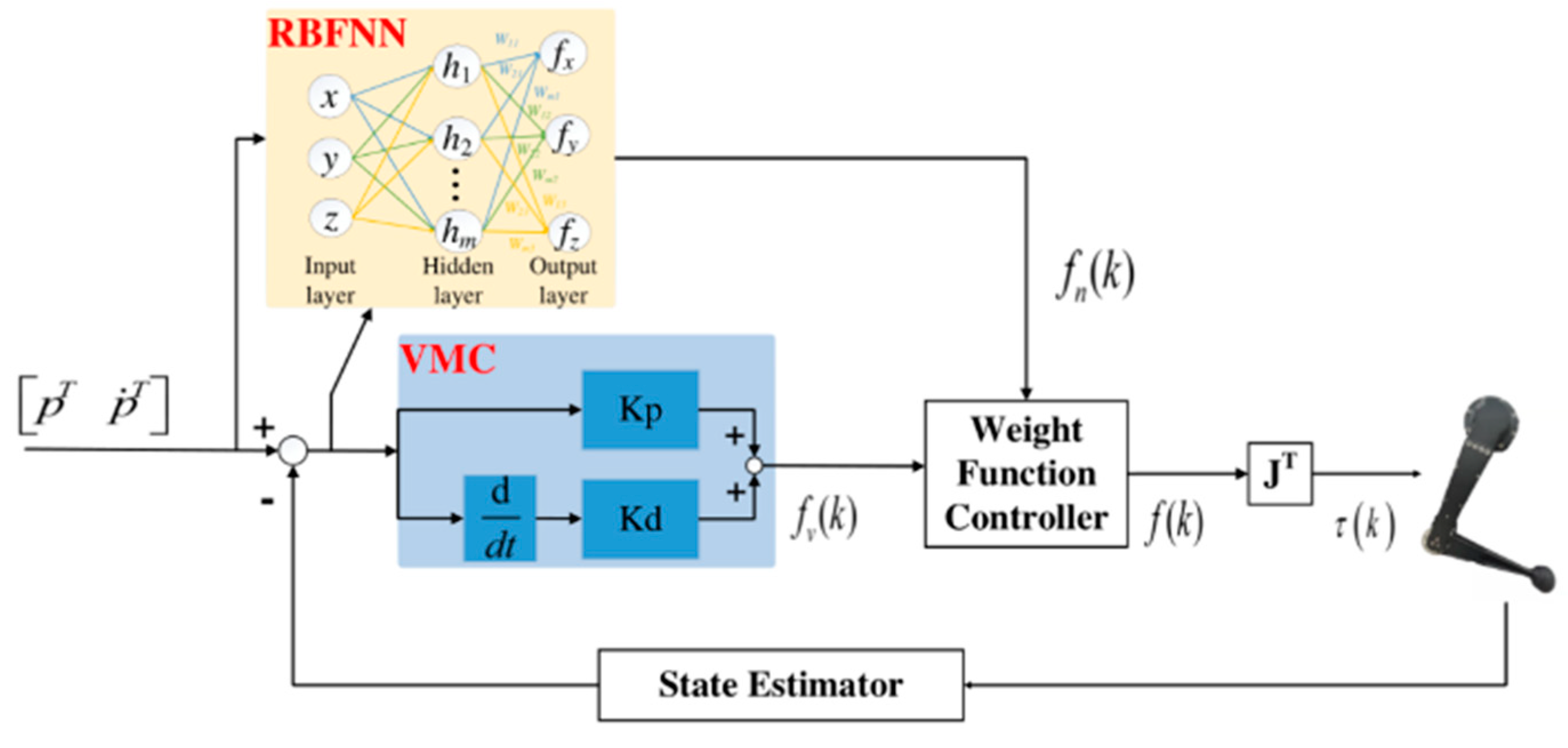
A swing leg controller is used to control the swinging motion at the foot-end for the robot. First, given the initial point where the foot-end leaves the ground, the highest point and the swing period, and then the integration of the motion velocity to solve for the position of the landing point, the desired Bezier trajectory of the foot-end is planned. Secondly, a virtual spring-damping system is used to obtain the output force at the foot-end. At the same time, a supervisory controller based on RBFNN is designed as the feedforward team for the SLC, and online learning is performed to optimize the parameters. Finally, the outputs of the two controllers are coordinated by a weight function to achieve fast and accurate tracking for the desired trajectory. The SLC architecture is shown in Figure 4.

3.3.1. Virtual Model Control

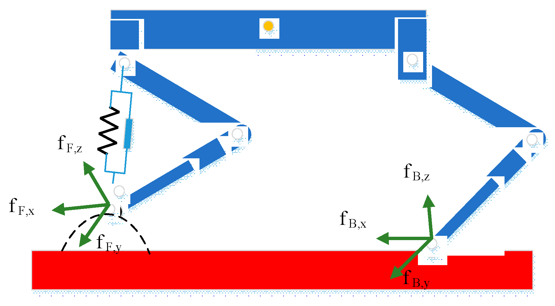
The foot-end swing control for the quadruped robot based on VMC is realized by adding a virtual spring-damping model between the swing foot and the desired foot-end position. When the desired foot-end position changes over time, the model will pull the swing leg to follow the foot trajectory. The virtual spring-damping model for the swing leg is shown in Figure 5, and the mathematical expression is (21).

$$\{\begin{array}{c}{f}_x=K{p}_x\left(x-x_d\right)+K{d}_x\left(\dot{x}-{\dot{x}}_d\right)\\ f_y=K{p}_y\left(y-y_d\right)+K{d}_y\left(y-{\dot{y}}_d\right)\\ f_z=K{p}_z\left(z-z_d\right)+K{d}_z\left(\dot{z}-{\dot{z}}_d\right)\end{array}$$

(21)

where $Kp$ and $Kd$ are the spring and damping coefficients, respectively. By adjusting them, the spring effects with different characteristics can be simulated.

The torque of each joint for the swinging leg is obtained by the Jacobi matrix. According to the principle of virtual work, the relationship between the space force and the motor torque can be obtained as follows:

$$\left[\begin{array}{c}{\tau }_1\\ {\tau }_2\\ {\tau }_3\end{array}\right]=J{F}^T=\left[\begin{array}{ccc}\frac{\partial x}{\partial {\theta }_1}& \frac{\partial y}{\partial {\theta }_1}& \frac{\partial z}{\partial {\theta }_1}\\ \frac{\partial x}{\partial {\theta }_2}& \frac{\partial y}{\partial {\theta }_2}& \frac{\partial z}{\partial {\theta }_2}\\ \frac{\partial x}{\partial {\theta }_3}& \frac{\partial y}{\partial {\theta }_3}& \frac{\partial z}{\partial {\theta }_3}\end{array}\right]\left[\begin{array}{c}{f}_x\\ f_y\\ f_z\end{array}\right]$$

(22)

3.3.2. RBFNN Supervision Control

RBFNN is a three-layer feedforward network with a single hidden layer, which has been proven to be able to approximate any continuous function with arbitrary precision. The structure of a multiple input multiple output neural network is shown in Figure 6. The first layer is the input layer, and the number of nodes is equal to the dimension of the input. The second layer is a hidden layer, and the number of nodes depends on the complexity of the problem, and the radial basis function is used as the basis function. The third layer is the output layer, and the number of nodes equals the dimension of the output data [42,43].

The radial basis vector is $h=[h_1,\dots ,h_m{]}^T$, $h_{\mathrm{j}}$ is the output of the neuron in the hidden layer.

$$h_{\mathrm{j}}=\exp (-\frac{{\Vert x-c_j\Vert }^2}{2b_j{}^2})$$

(23)

where $c=\left[c_{ij}\right]=\left[\begin{array}{ccc}{c}_{11}& \cdots & c_{1m}\\ ⋮& \ddots & ⋮\\ c_{n1}& \cdots & c_{nm}\end{array}\right]$ is the coordinate vector of the Gaussian basis function centroid for the j-th neuron in the hidden layer; $b=[b_1,\dots ,b_m{]}^T$, $b_j$ is the width of the Gaussian basis function for the j-th neuron in the hidden layer.

The weight of RBFNN is:

$$\omega =\left[{\omega }_{ij}\right]=\left[\begin{array}{ccc}{\omega }_{11}& \cdots & {\omega }_{1m}\\ ⋮& \ddots & ⋮\\ {\omega }_{n1}& \cdots & {\omega }_{nm}\end{array}\right]$$

(24)

The output of RBFNN is:

$$f_{\mathrm{i}}={\displaystyle \sum _{j=1}^m{\omega }_{i{\mathrm{j}}_{}^{}}{h}_j},i=1,2,\cdots ,n$$

(25)

Setting the expected tracking instruction as $y$; the RBFNN performance index function is:

$$E(k)=\frac{1}{2}e{(k)}^2=\frac{1}{2}(y(k)-f(k){)}^2$$

(26)

According to the gradient descent method, the iterative control algorithm of output weight, node base width and center vector parameters are as follows [44,45]:

$$\Delta {\omega }_{\mathrm{j}}(k)=-\eta \frac{\partial E(k)}{\partial b_j}=\eta e(k)\frac{\partial y(k)}{\partial u(k)}{h}_j$$

(27)

$${\omega }_{\mathrm{j}}(k)={\omega }_{\mathrm{j}}(k-1)+\Delta {\omega }_{\mathrm{j}}(k)+\alpha \Delta {\omega }_{\mathrm{j}}(k)$$

(28)

$$\Delta {\mathrm{b}}_{\mathrm{j}}(k)=-\eta \frac{\partial E(k)}{\partial b_j}=\eta e(k)\frac{\partial y(k)}{\partial u(k)}\frac{\partial u(k)}{\partial b_j}=\eta e(k)\frac{\partial y(k)}{\partial u(k)}{\omega }_j{h}_j\frac{{\Vert x-c_{ij}\Vert }^2}{b_j{}^3}$$

(29)

$$b_{\mathrm{j}}(k)=b_{\mathrm{j}}(k-1)+\eta \Delta b_{\mathrm{j}}(k)+\alpha (b_{\mathrm{j}}(k-1)-b_{\mathrm{j}}(k-2))$$

(30)

$$\Delta c_{\mathrm{ij}}(k)=-\eta \frac{\partial E(k)}{\partial c_{\mathrm{ij}}}=\eta e(k)\frac{\partial y(k)}{\partial u(k)}\frac{\partial u(k)}{\partial c_{\mathrm{ij}}}=\eta e(k)\frac{\partial y(k)}{\partial u(k)}{\omega }_j{h}_j\frac{x-c_{ij}}{b_j{}^2}$$

(31)

$$c_{ij}(k)=c_{ij}(k-1)+\eta \Delta c_{ij}(k)+\alpha (c_{ij}(k-1)-c_{ij}(k-2))$$

(32)

where $\frac{\partial y(k)}{\partial u(k)}$ the Jacobian matrix, represents the sensitivity of the system output to the control input.

3.3.3. Weight Function Controller

Since both the VMC Controller and the RBF Controller have the ability to track foot-end trajectory, the weighting factor $T_i$ is introduced to design the Weight Function Controller (WFC) in order to obtain a better control effect [46,47]. When the tracking error is large, the VMC controller and the RBF controller are used at the same time. When the tracking error is small, only the VMC controller is used.

We define the instantaneous error performance index $CE$ and the average error performance index $DE$ for foot-end trajectory tracking as shown below:

$$CE=\sqrt{{(x-x_d)}^2+{(y-y_d)}^2+{(z-z_d)}^2}$$

(33)

$$DE=\frac{{\displaystyle \sum _{i=1}^{N}C{E}_i}}{N}$$

(34)

Define the weighting factor $T_i$:

$$T_1=\{\begin{array}{c}1\\ 1-\left(\left|CE\right|-E_1\right)/\left(E_2-E_1\right)\\ 0\end{array}\begin{array}{c}\left|CE\right|>E_2\\ E_2>\left|CE\right|>E_1\\ \left|CE\right|<E_1\end{array}$$

(35)

$$T_2=1$$

(36)

where $E_1$ and $E_2$ are the two thresholds for the instantaneous error performance index; when $\left|CE\right|<E_1$, only the VMC controller is used; when $E_2>\left|CE\right|>E_1$, the influence of the RBF controller is gradually weakened; when $\left|CE\right|>E_2$, both the VMC controller and the RBF controller are used. Then the final control outputs for SLC are:

$$\tau =J{\left(T_1{f}_n+T_2{f}_v\right)}^{\mathrm{T}}$$

(37)

where $f_n$ and $f_v$ are the control outputs of the RBF controller and the VMC controller, respectively. After debugging, it is found that when $E_1=0.005$ and $E_2=0.04$, the control effect for the system is the best.

4. Experimental Results

4.1. Quadruped Robot Experimental Platform

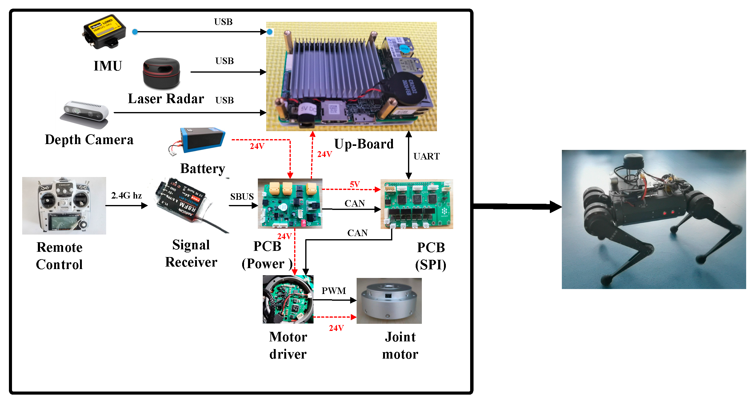
A medium-sized quadruped robot was built in the laboratory, whose internal hardware structure, communication method and shape are shown in Figure 7. Each leg is composed of three joint motors, responsible for one Degree of Freedom (DoF) in traverse roll and two DoF in pitch. The internal hardware structure is based on the Up-Board as the control core, the inertial measurement unit, laser radar and depth camera as the robot state monitoring device, the motor drive version as the drive unit; the brushless DC motor as the execution unit, and the SPI circuit board as the signal conversion board from the Up-Board to the motor driver. Lithium-ion batteries and power boards provide the power needed for each module. The hardware structure relationship is that it receives the expected command information of the remote controller, and then calculates the torque control amount for the robot in real time according to the state information, such as the angle, position, velocity and centroid attitude of each joint and foot-end. The motor driving board controls the rotation angle, speed and torque through different currents to realize the movement of the quadruped robot. The physical parameters of the quadruped robot are shown in

Table 1. Physical parameters of quadruped robot.

Parameters	Symbol	Values	Units
Body mass	m	3.3	kg
Gravitational acceleration	g	9.8	m/s2
Body Inertia	Ixx	0.35	kg × m2
Body Inertia	Iyy	2.1	kg × m2
Body Inertia	Izz	2.1	kg × m2
Body length	Lbody	0.37	m
Body width	Wbody	0.11	m
Body height	Hbody	0.1	m
Ab/Ad link length	L1	0.072	m
Upper link length	L2	0.211	m
Lower link length	L3	0.2	m
Sampling period	T	15	ms

.

4.2. Initial Value Training of RBFNN Controller

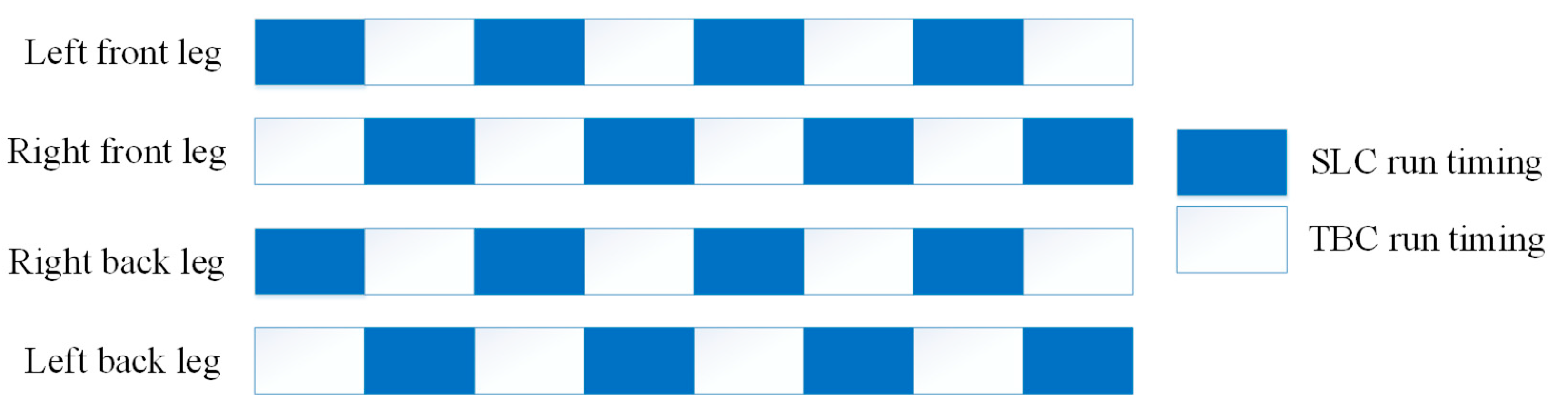
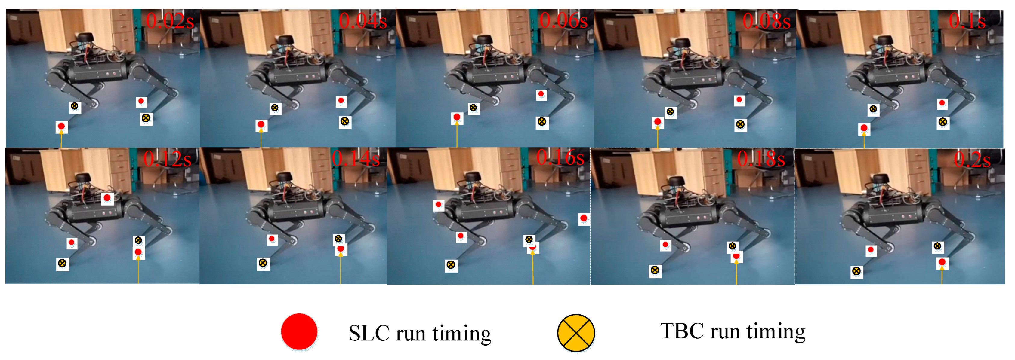
The diagonal trotting gait is one of the most efficient motions for quadruped robots, which takes into account both stability and velocity [48]. Therefore, the controller designed in this paper is tested in this gait. A four-legged timing diagram for diagonal trotting motion is shown in Figure 8 and Figure 9. Two legs on the diagonal of the robot’s trunk are in the same phase in this gait, while two legs on the other diagonal are in the opposite phase. The TBC and SLC are continuously switched on each leg, enabling the robot to maintain dynamic stability during periods of rapid motion.

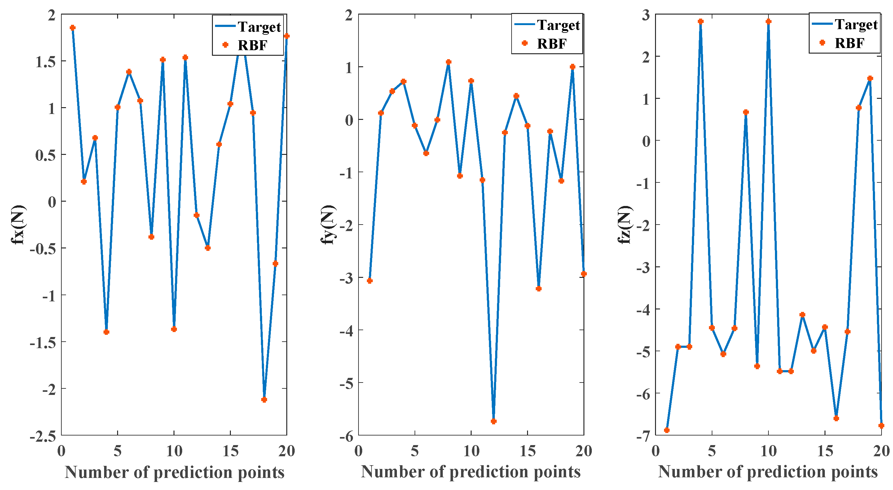
To ensure the effectiveness of the RBFNN controller, the initial values of $\omega$, $\mathrm{b}$ and $c$ need to be trained before testing. The training data set is composed of 800 pairs of the expected position of the foot-end trajectory using only the VMC and the corresponding foot-end virtual force output. After the controller training is completed, 20 sets of data are randomly selected for prediction, the test data is shown in Figure 10, the RBFNN controller was able to output the correct target virtual force and achieved the design requirements for the controller.

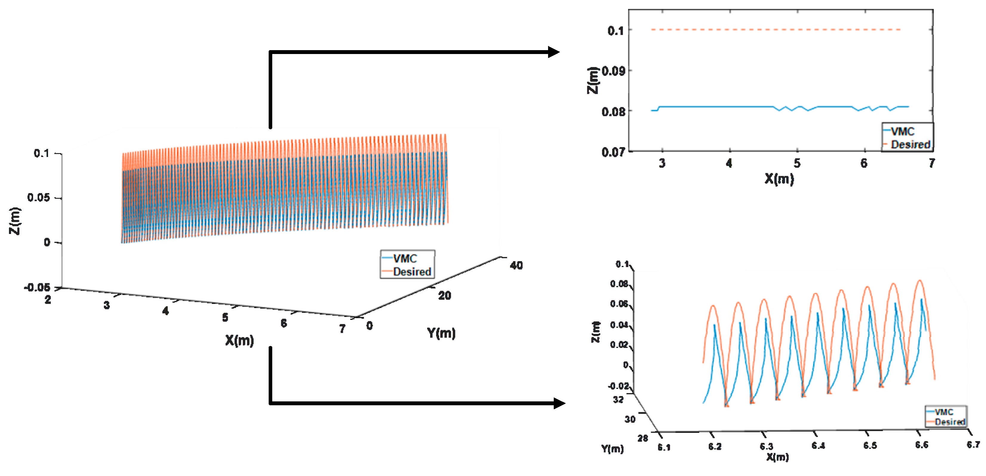
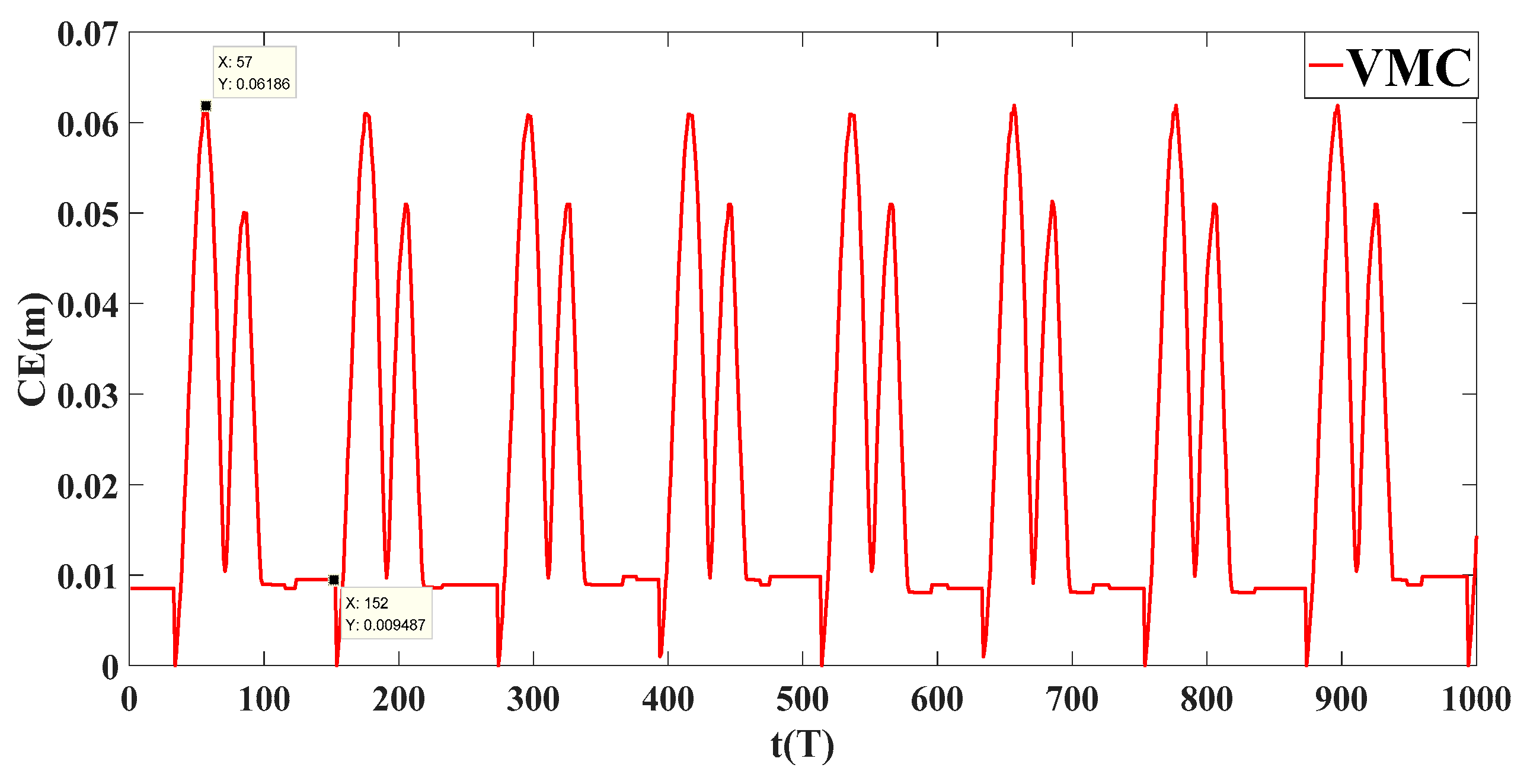
As shown in Figure 11, when only the VMC controller is used for foot-end trajectory tracking, there is always a tracking error close to 0.02 m in the Z-axis direction. The instantaneous error CE index is shown in Figure 12. The maximum and minimum CE performance index for the robot is 0.062 and 0.01, respectively, and the DE index is 0.022.

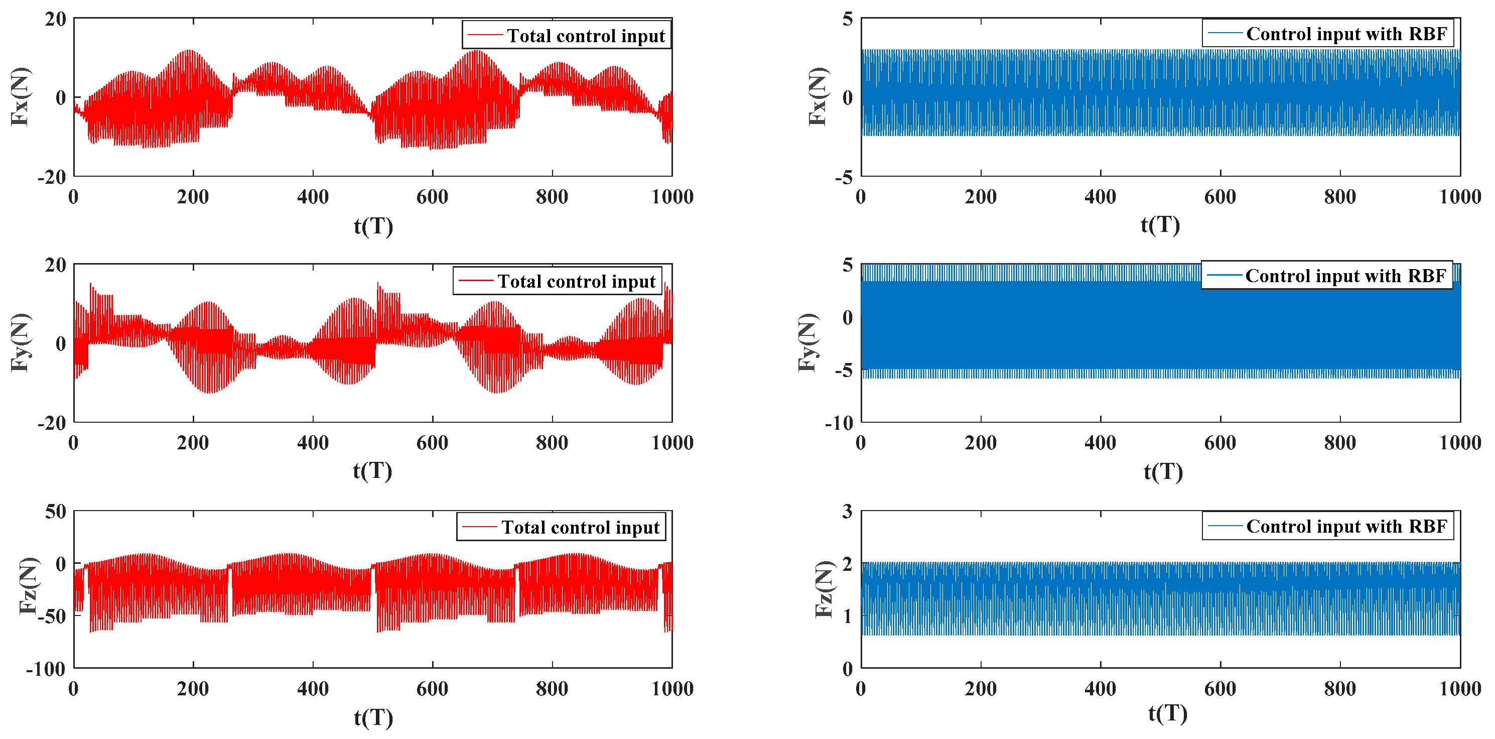
The RBF + VMC controller is used for foot-end trajectory tracking experiments, and the RBF controller supervises and compensates for the VMC controller. The total amount of virtual force output and the amount of virtual force compensation at the foot-end are shown in Figure 13, it can be found that the virtual force input of the quadruped robot is the same in each swing phase when trotting on a smooth road, and the minimum virtual force in the vertical axis fluctuates around 0. This is because the foot-end trajectory uses a Bessel curve, and the acceleration is 0 at the highest point, while the acceleration is maximum when touching the ground.

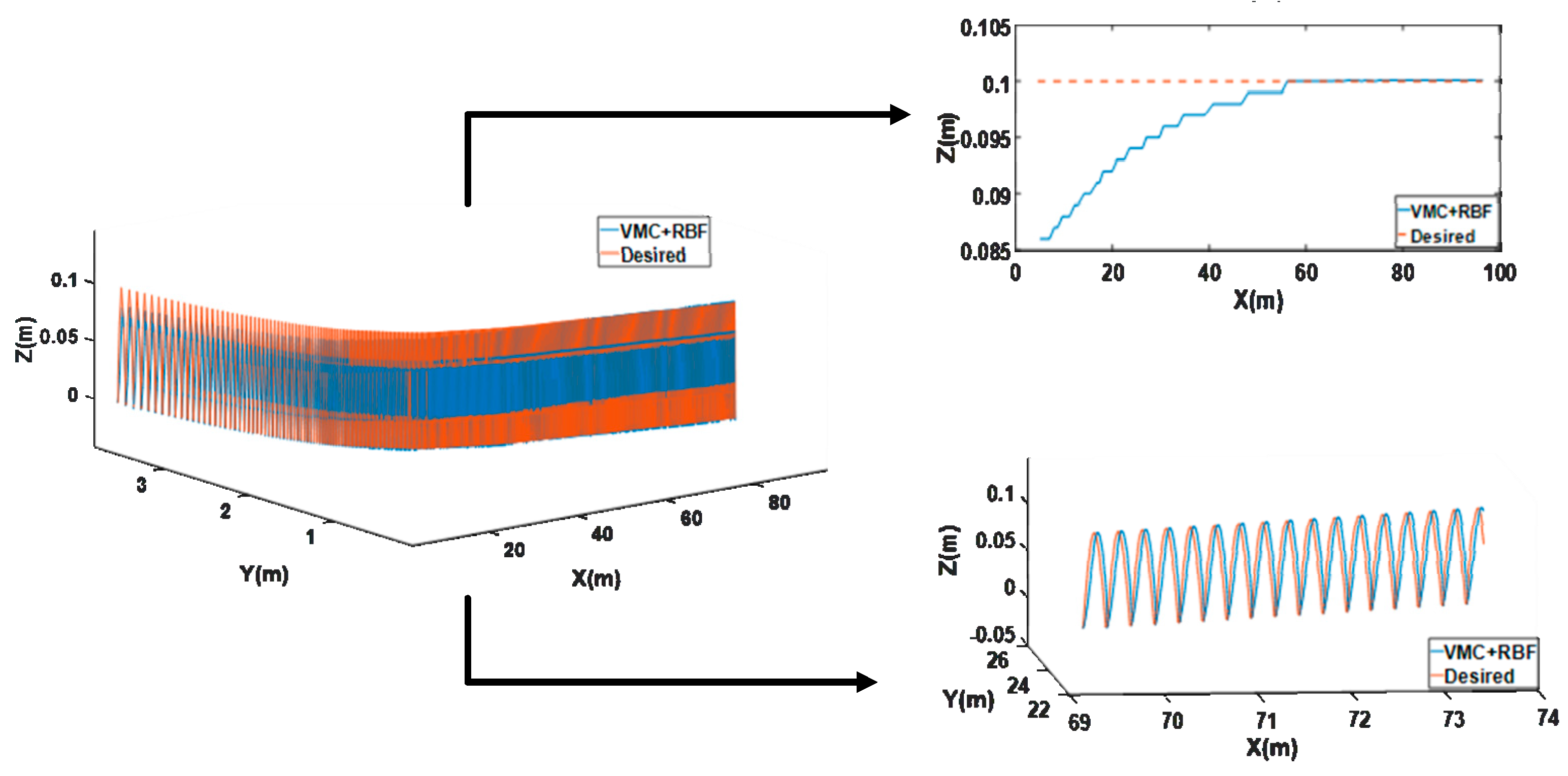
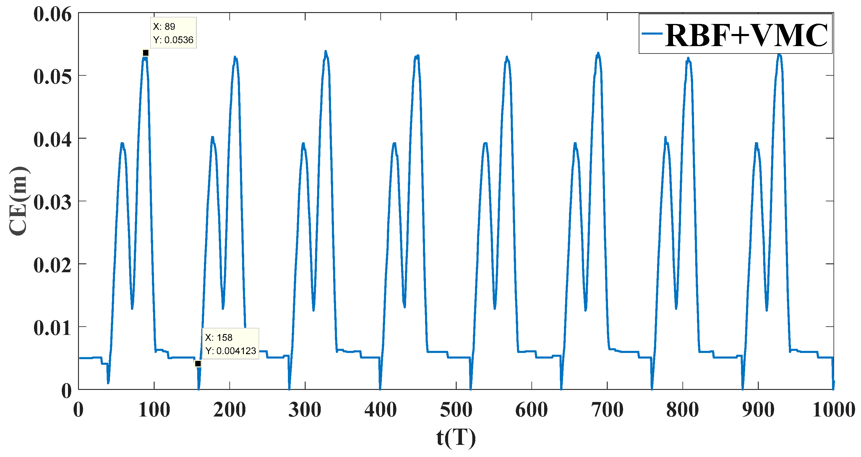
The experimental results are shown in Figure 14. The foot-end gradually tracks the desired trajectory and the steady-state error is gradually eliminated. The instantaneous error CE index is shown in Figure 15. The error index for the VMC+RBF controller is lower than that of the VMC controller, which is 0.0536 and 0.004, respectively. In addition, the DE error index for the VMC+RBF controller is 0.0177, which is 19.55% lower than that of the VMC controller.

4.3. COM Trajectory Tracking Experiment

4.3.1. Linear Trajectory Tracking Experiment

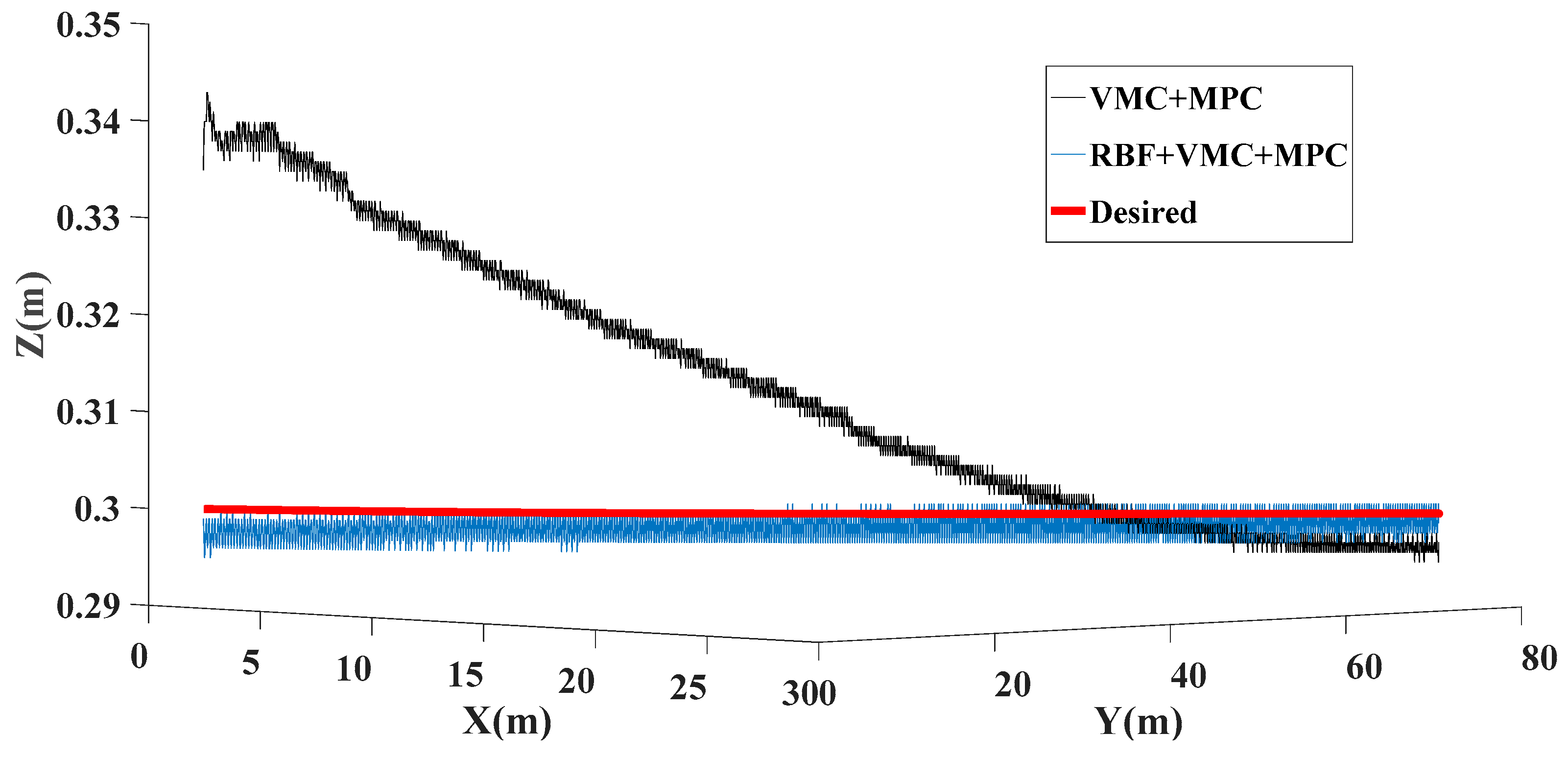
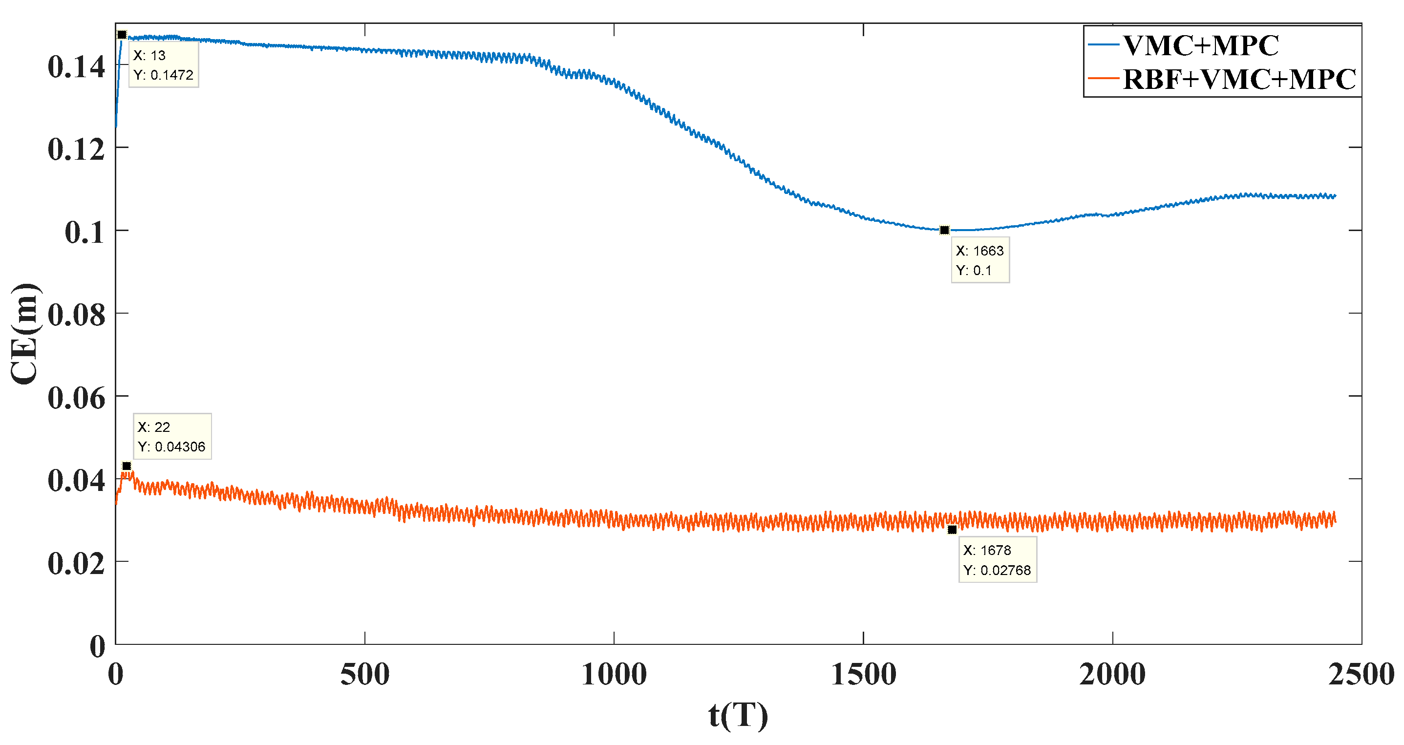
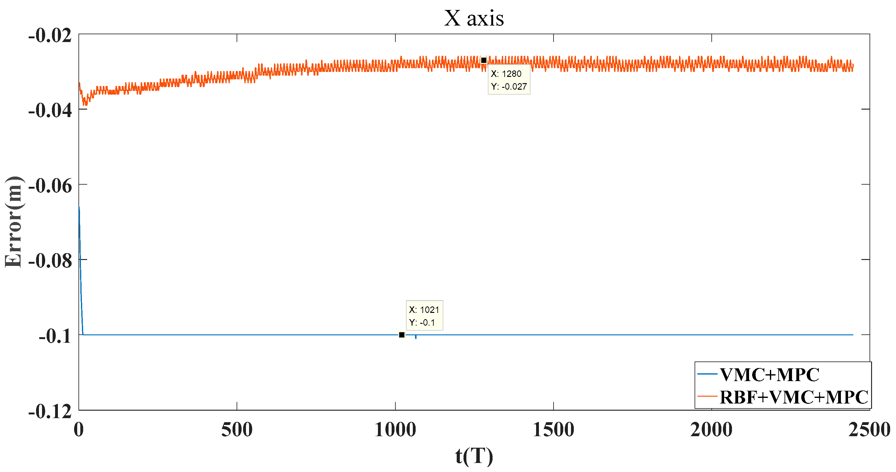
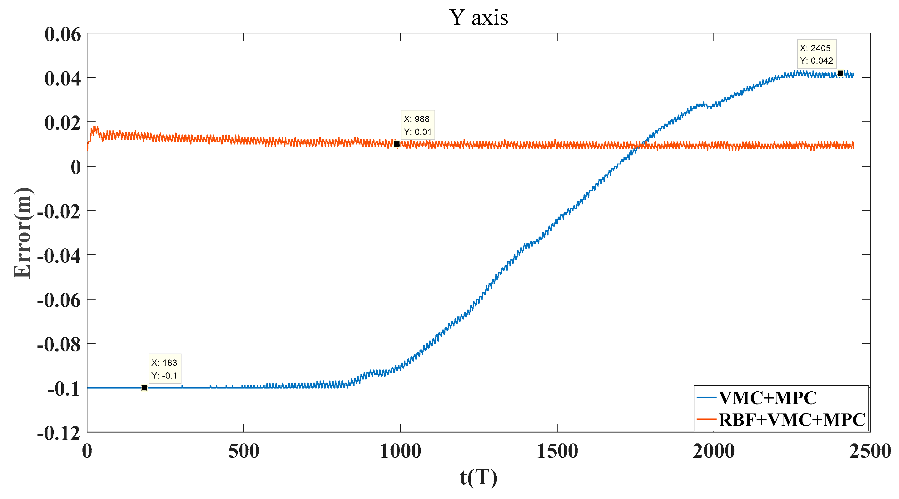
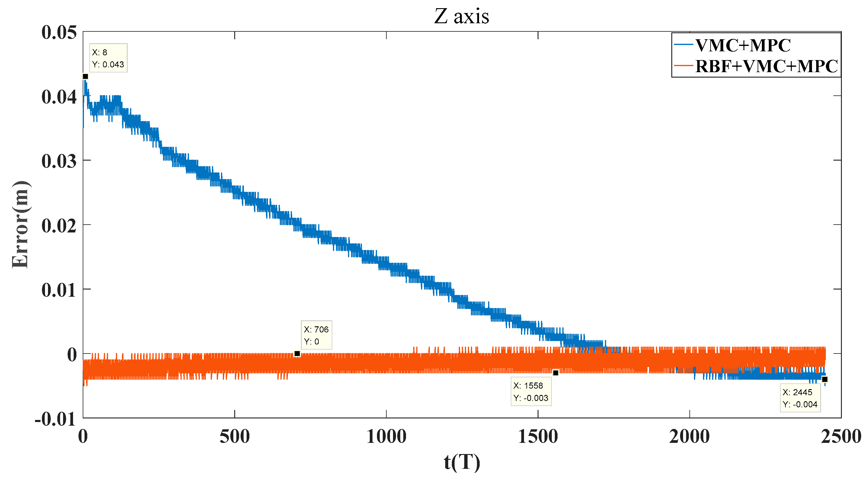
The quadruped robot performs linear trajectory tracking at a speed of 2.5 m/s. As shown in Figure 16, the VMC+MPC controller has a large tracking error and slow convergence. After using the RBF+VMC+MPC controller, the tracking trajectory can be significantly improved, which can achieve fast and accurate tracking, at the same time, the whole trajectory tracking process is stable. The specific index of the whole tracking process was analyzed, as shown in Figure 17, Figure 18, Figure 19 and Figure 20. When the VMC+MPC controller was used, the index of CE fluctuated between 0.1 m and 0.1472 m, and the index of DE was 0.1228 m. After RBF controller compensation, the index parameter of CE was stable at 0.0277 m, and the DE index is 0.0314 m, which is 74.43% lower than that of the VMC+MPC controller. The X-axis tracking error is −0.1 m when the VMC+MPC controller is used and decreases to −0.027 m after the RBF controller is used to compensate. The tracking error of the Y-axis fluctuates from −0.1 m to 0.042 m when the VMC+RBF controller is used, but after compensating by the RBF controller, the tracking error is stable at 0.01 m. The Z-axis tracking error fluctuates from 0.043 m to −0.004 m when the VMC+MPC controller is used. After compensating by the RBF controller, the tracking error is stabilized within 0 to −0.003 m. Therefore, for linear trajectory tracking for quadruped robots, the tracking control method designed in this paper has the advantages of high accuracy performance, small fluctuation range and high steady-state performance.

4.3.2. Circular Trajectory Tracking Experiment

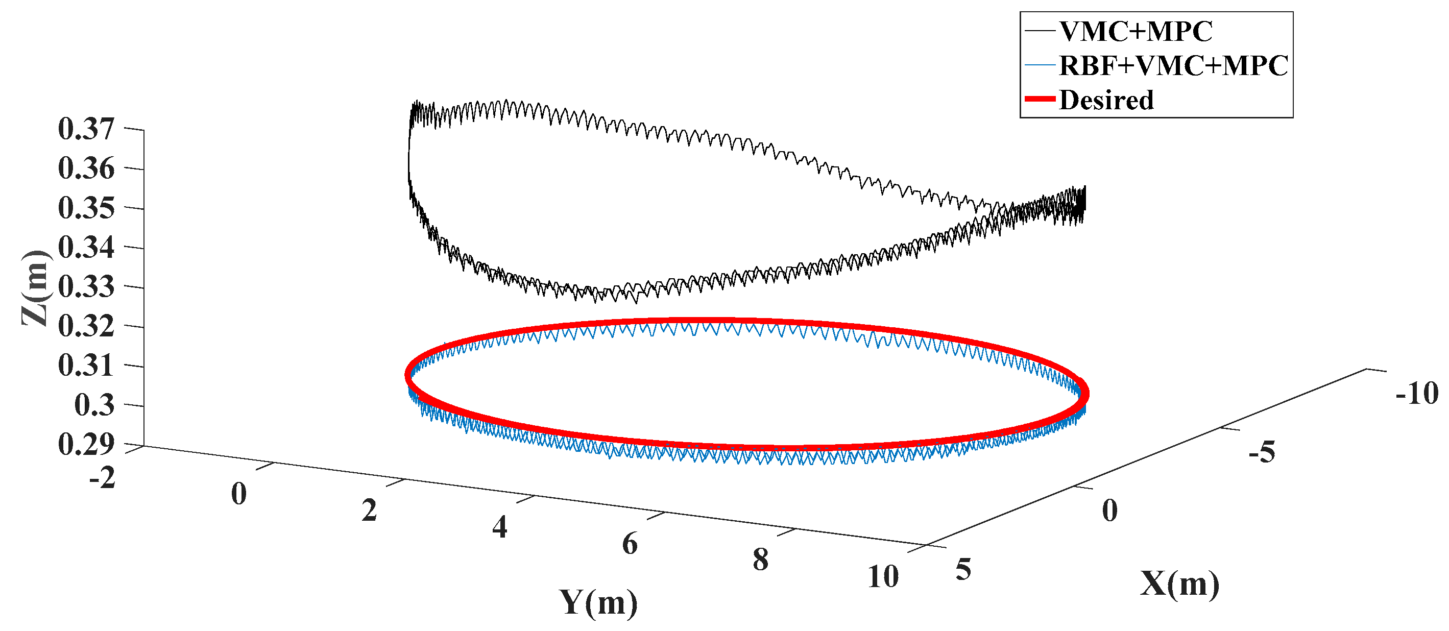
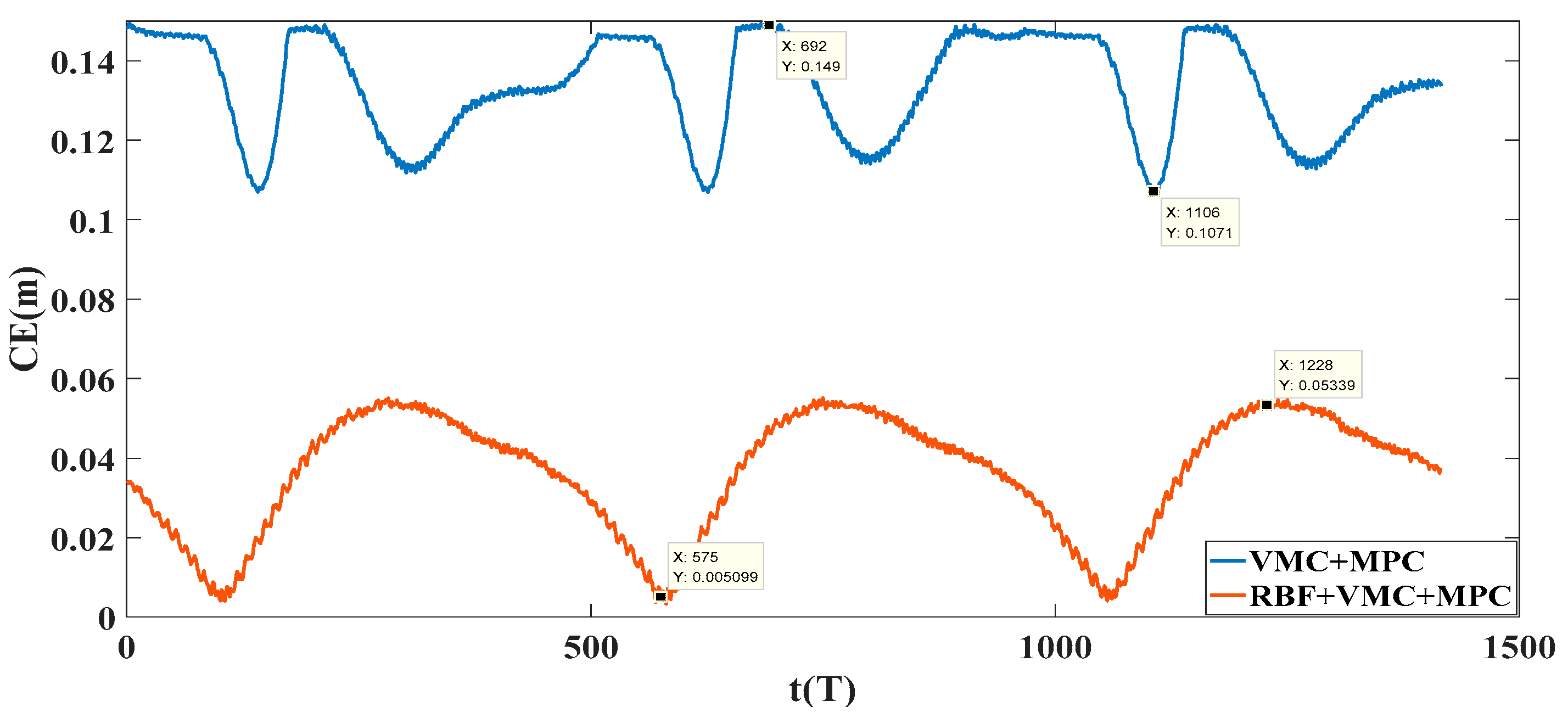
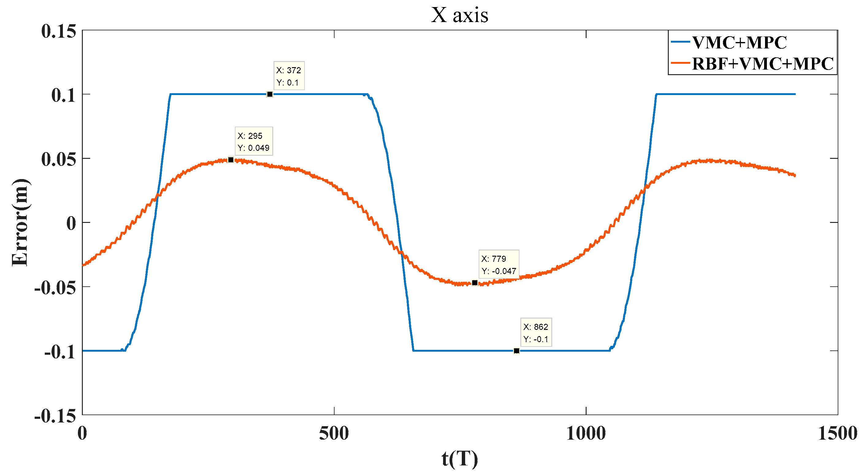
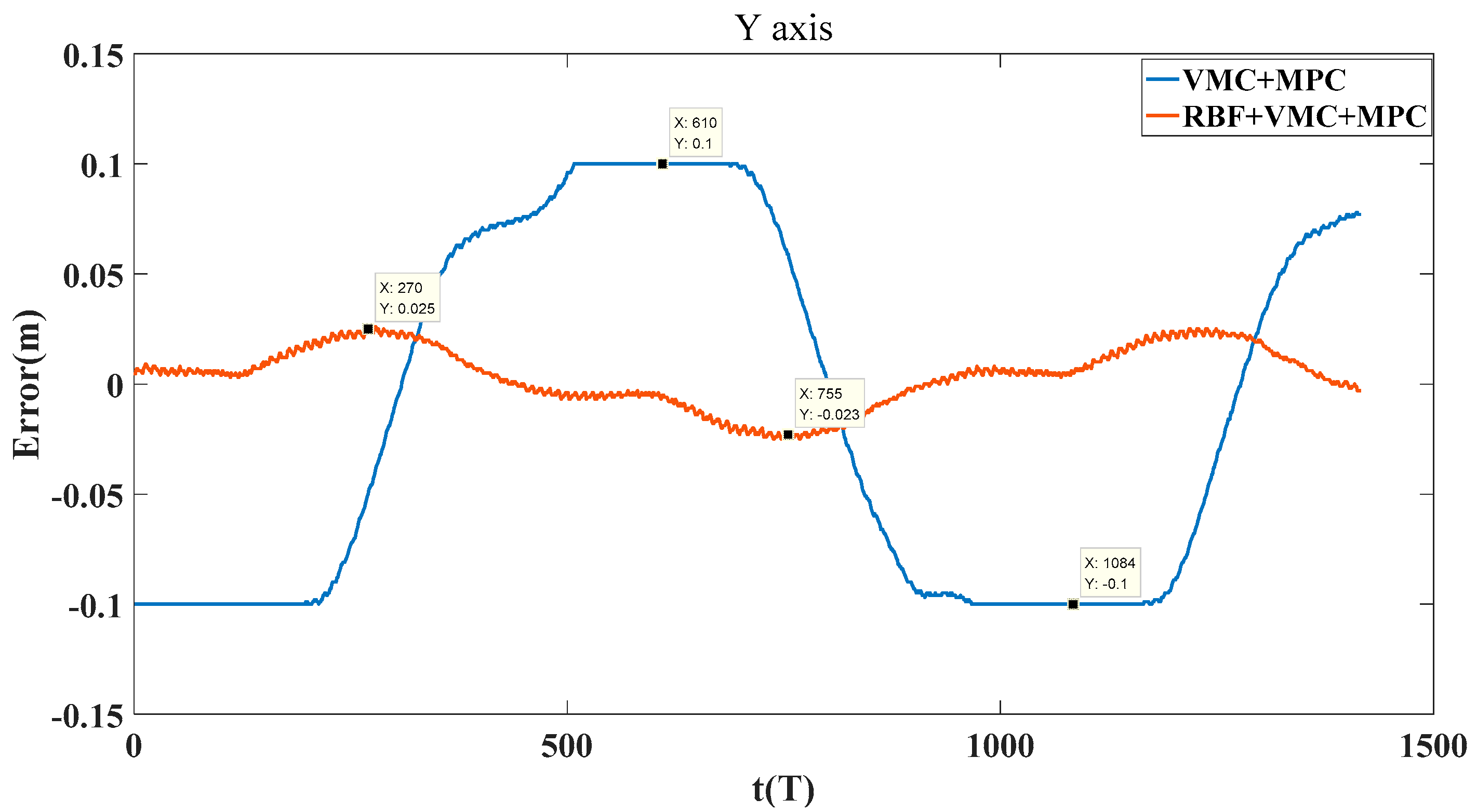
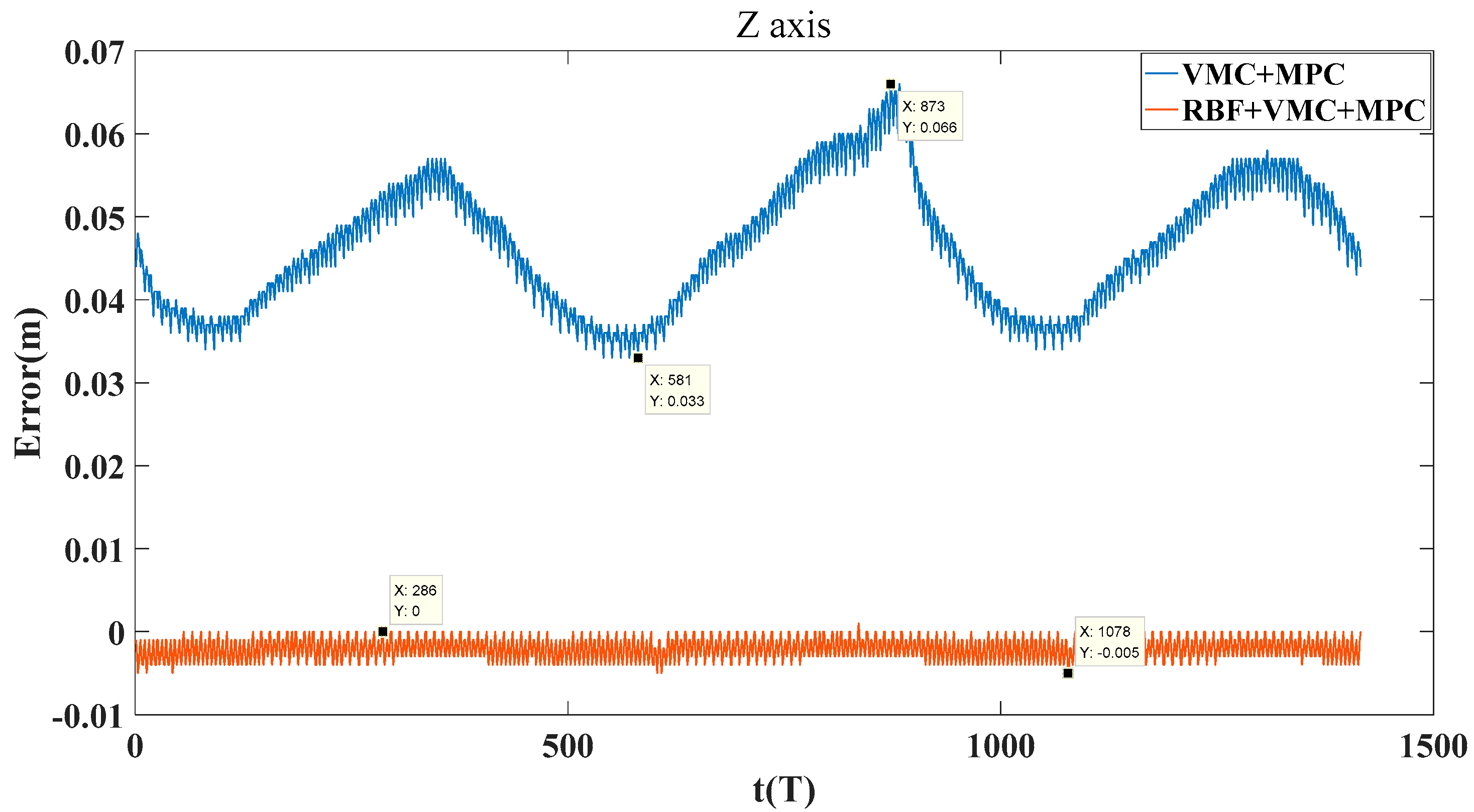
The quadruped robot performs circular trajectory tracking at a speed of 2.5 m/s, as shown in Figure 21. When using the VMC + MPC controller, there is a large tracking error, the tracking trajectory has large fluctuations. After using the RBF + VMC + MPC controller, the tracking effect can be significantly improved, which can achieve fast and accurate tracking, as well as stable operation of the whole trajectory tracking process. We analyzed specific indicators during the whole tracking process, as shown in Figure 22, Figure 23, Figure 24 and Figure 25. When the VMC + MPC controller is used, the CE index fluctuates between 0.1071 m and 0.149 m, and the index of DE is 0.1336. After RBF controller compensation, the CE index was stable between 0.0051 m and 0.0534 m, DE index value was 0.0363, compared with the VMC + MPC controller DE index decreased by 72.83%. When using the VMC + MPC controller, the X-axis tracking error fluctuates between −0.1 m and 0.1 m and decreases to −0.047 m and 0.049 m after compensating by the RBF controller. When the VMC + MPC controller is used, the tracking error of the Y-axis fluctuates between −0.1 m and 0.1 m, and after compensation by the RBF controller, the tracking error is reduced to fluctuation between −0.023 m and 0.025 m. When the VMC+MPC controller is used, the tracking error of the Z-axis fluctuates between 0.033 m and 0.066 m. After compensation by the RBF controller, the tracking error is reduced to fluctuation between −0.005 m and 0. Therefore, for the circular trajectory tracking of quadruped robots, the tracking control method designed in this paper can improve the accuracy of trajectory tracking and has the advantages of a small fluctuation range and high steady-state performance.

5. Conclusions

In this paper, a new trajectory tracking control method for quadruped robots is designed. The method establishes TBC based on MPC theory and SWL based on RBFNN and virtual models, respectively. The TBC completes two aspects of the predictive model and the optimal solution for the trajectory tracking of the quadruped robot according to the MPC theory. The SLC combines the advantages of the virtual model and RBFNN, and the VMC controller and RBFNN controller are designed, respectively, and the outputs of the two controllers are coordinated with a weight function. The control method of this paper has been experimentally verified: the foot-end trajectory tracking experiments show that the control method solves the problems of steady-state error and unsatisfactory tracking effect of conventional VMC methods; the linear and circular trajectory tracking experiments with COM shows the control method can achieve fast and accurate tracking for desired trajectories, which can meet the control requirements of quadruped robot and is easy apply in engineering.

References

- Choi, J. Multi-Phase Joint-Angle Trajectory Generation Inspired by Dog Motion for Control of Quadruped Robot. Sensors 2021, 21, 6366. [Google Scholar] [CrossRef] [PubMed]
- Rodino, S.; Matteo Curcio, E.; di Bella, A.; Persampieri, M.; Funaro, M.; Carbone, G. Design, Simulation, and Preliminary Validation of a Four-Legged Robot. Machines 2020, 8, 82. [Google Scholar] [CrossRef]
- Liu, J.; Tan, M.H.; Zhao, X. Legged robots—An overview. Trans. Inst. Meas. Control 2007, 29, 185–202. [Google Scholar] [CrossRef]
- Wang, J.H.; Wen, J.T.; Chen, W.H.; Yue, H.S.; Liu, D. A gait generating algorithm with smooth speed transition for the locomotion of legged robots. Trans. Inst. Meas. Control 2014, 36, 260–275. [Google Scholar] [CrossRef]
- Li, J.; Cong, D.; Yang, Y.; Yang, Z. A new bionic hydraulic actuator system for legged robots with impact buffering, impact energy absorption, impact energy storage, and force burst. Robotica 2021, 56, 1–18. [Google Scholar] [CrossRef]
- Kang, R.; Meng, F.; Wang, L.; Chen, X.; Yu, Z.; Fan, X.; Sato, R.; Ming, A.; Huang, Q. Bio-Inspired Take-Off Maneuver and Control in Vertical Jumping for Quadruped Robot with Manipulator. Micromachines 2021, 12, 1189. [Google Scholar] [CrossRef]
- Chen, X.D.; Watanabe, K.; Kiguchi, K.; Izumi, K. Path tracking based on closed-loop control for a quadruped robot in a cluttered environment. J. Dyn. Syst. Meas. Control 2002, 124, 272–280. [Google Scholar] [CrossRef]
- Oliveira, I.; Barbosa, R.; Silva, M. Modelling, Trajectory Planning and Control of a Quadruped Robot Using Matlab®/Simulink™. In Proceedings of the ROBOT 2017: Third Iberian Robotics Conference, Advances in Intelligent Systems and Computing, Sevilla, Spain, 22–24 November 2017; Volume 694, pp. 757–767. [Google Scholar] [CrossRef]
- Chen, B.; Pei, Z.C.; Tang, Z.Y. Adaptive fuzzy PID control for hydraulic quadruped robot. J. Harbin Inst. Technol. 2016, 48, 140–144. [Google Scholar] [CrossRef]
- Pratt, J.; Dilworth, P.; Pratt, G. Virtual model control of a bipedal walking robot. In Proceedings of the International Conference on Robotics and Automation, Albuquerque, NM, USA, 25 April 1997; Volume 1, pp. 193–198. [Google Scholar] [CrossRef]
- Liu, B.; Rong, X.; Chai, H. A buffering strategy for quadrupedal robots based on virtual model control. Robot 2016, 38, 659–669. [Google Scholar] [CrossRef]
- Chen, G.; Guo, S.; Hou, B. Virtual model control for quadruped robots. IEEE Access 2020, 8, 140736–140751. [Google Scholar] [CrossRef]
- Boaventura, T.; Buchli, J.; Semini, C.; Caldwell, D.G. Model-based hydraulic impedance control for dynamic robots. IEEE Trans. Robot. 2015, 31, 1324–1336. [Google Scholar] [CrossRef] [Green Version]
- Winkler, A.W.; Mastalli, C.; Havoutis, I.; Focchi, M.; Caldwell, D.G.; Semini, C. Planning and execution of dynamic whole-body locomotion for a hydraulic quadruped on challenging terrain. In Proceedings of the 2015 IEEE International Conference on Robotics and Automation, ICRA, Seattle, WA, USA, 26–30 May 2015; pp. 5148–5154. [Google Scholar] [CrossRef] [Green Version]
- Zhang, G.T.; Rong, X.W.; Hui, C.; Li, Y.; Li, B. Torso motion control and toe trajectory generation of a trotting quadruped robot based on virtual model control. Adv. Robot. 2016, 30, 284–297. [Google Scholar] [CrossRef]
- Zhang, G.T.; Rong, X.W.; Li, Y.B.; Cai, H.; Li, B. Gait control method of quadruped robot diagonal trot based on virtual model. Robot 2016, 38, 64–74. [Google Scholar] [CrossRef]
- Luo, B. Balance control based on six-dimensional spatial mechanics and velocity adjustment through region intervention and foot landing for quadruped robot. Robotica 2022, 89, 1–23. [Google Scholar] [CrossRef]
- Kurazume, R.; Byong-Won, A.; Ohta, K.; Hsutomu, H. Experimental study on energy efficiency for quadruped walking vehicles. In Proceedings of the IEEE/RSJ International Conference on Intelligent Robots & Systems, Las Vegas, NV, USA, 27–31 October 2003; pp. 613–618. [Google Scholar] [CrossRef]
- Si, Z.; Gao, J.; Duan, X.; Li, H. Trot pattern generation for quadruped robot based on the ZMP stability margin. Int. Conf. Complex Med. Eng. 2013, 32, 603–608. [Google Scholar] [CrossRef]
- Hoang, G.; Kim, H.K.; Kim, S.B. Path tracking controller of quadruped robot for obstacle avoidance using potential functions method. Int. J. Sci. Eng. 2013, 4, 1–5. [Google Scholar] [CrossRef]
- Dini, N.; Majd, V.D. An MPC-based two-dimensional push recovery of a quadruped robot in trotting gait using its reduced virtual model. Mech. Mach. Theory 2019, 146, 1–25. [Google Scholar] [CrossRef]
- Carlo, J.D.; Wensing, P.M.; Katz, B.; Bledt, G.; Kim, S. Dynamic Locomotion in the MIT Cheetah 3 Through Convex Model-Predictive Control. In Proceedings of the 2018 IEEE/RSJ International Conference on Intelligent Robots and Systems (IROS), Madrid, Spain, 1–5 October 2018; pp. 7440–7447. [Google Scholar] [CrossRef]
- Bledt, G.; Powell, M.J.; Katz, B.; Carlo, J.D.; Wensing, P.M.; Kim, S. MIT Cheetah 3: Design and Control of a Robust, Dynamic Quadruped Robot. In Proceedings of the 2018 IEEE/RSJ International Conference on Intelligent Robots and Systems (IROS), Madrid, Spain, 1–5 October 2018; pp. 2245–2252. [Google Scholar] [CrossRef]
- Luan, F.; Na, J.; Huang, Y.; Gao, G. Adaptive neural network control for robotic manipulators with guaranteed finite-time convergence. Neurocomputing 2019, 337, 153–164. [Google Scholar] [CrossRef]
- Zhang, C.; Yang, Z.; Liao, L.; You, Y.; Sui, Y.; Zhu, T. RPEOD: A Real-Time Pose Estimation and Object Detection System for Aerial Robot Target Tracking. Machines 2022, 10, 181. [Google Scholar] [CrossRef]
- Hwangbo, J.; Lee, J.; Dosovitskiy, A.; Bellicoso, D.; Tsounis, V.; Koltun, V.; Hutter, M. Learning agile and dynamic motor skills for legged robots. Sci. Robot. 2019, 4, 831–849. [Google Scholar] [CrossRef] [Green Version]
- Chen, Y.Z.; Hou, W.Q.; Wang, J.; Wang, J.W.; Ma, H.X. A strategy for push recovery in quadruped robot based on reinforcement learning. In Proceedings of the 2015 34th Chinese Control Conference, CCC, Hangzhou, China, 28–30 July 2015; pp. 3145–3151. [Google Scholar] [CrossRef]
- Ma, Z.; Liang, Y.; Tian, H. Research on Gait Planning Algorithm of Quadruped Robot Based on Central Pattern Generator. In Proceedings of the 2020 39th Chinese Control Conference (CCC), Shenyang, China, 27–29 July 2020; pp. 3948–3953. [Google Scholar] [CrossRef]
- Ren, D.; Shao, J.; Sun, G. The complex dynamic locomotive control and experimental research of a quadruped-robot based on the robot trunk. Appl. Sci. 2019, 9, 3911. [Google Scholar] [CrossRef] [Green Version]
- Zhang, C.; Dai, J. Trot gait with twisting trunk of a metamorphic quadruped robot. J. Biomim. Eng. Engl. Ed. 2018, 15, 971–981. [Google Scholar] [CrossRef]
- Atique, M.; Sarker, M.; Ahad, M. Development of an 8dof quadruped robot and implementation of inverse kinematics using denavit-hartenberg convention. Heliyon 2018, 4, 1–9. [Google Scholar] [CrossRef] [PubMed] [Green Version]
- Chang, X.; An, H.; Ma, H. Modeling and base parameters identification of legged robots. Robotica 2022, 40, 747–761. [Google Scholar] [CrossRef]
- Zhou, F.L.; You, Y.L.; Li, G. Study on singular trajectory method of inverse kinematics of space 3R manipulator. Mech. Sci. Technol. 2019, 38, 365–372. [Google Scholar] [CrossRef]
- Bledt, G.; Wensing, P.M.; Ingersoll, S.; Ingersoll, S.; Kim, S. Contact Model Fusion for Event-Based Locomotion in Unstructured Terrains. In Proceedings of the 2018 IEEE International Conference on Robotics & Automation, Brisbane, Australia, 21–25 May 2018; pp. 4399–4406. [Google Scholar] [CrossRef] [Green Version]
- Hu, N.; Li, S.; Huang, D.; Gao, F. Trotting gait planning for a quadruped robot with high payload walking on irregular terrain. IFAC Proc. Vol. 2014, 47, 2153–2158. [Google Scholar] [CrossRef] [Green Version]
- Han, B.; Luo, X.; Zhao, R.; Luo, Q.; Liang, G. The optimization algorithm for gait planning and foot trajectory on the quadruped robot. In Proceedings of the International Conference on Geometry and Graphics, Milan, Italy, 3–7 August 2018; pp. 1274–1279. [Google Scholar] [CrossRef]
- Ding, Y.; Pandala, A.; Li, C.; Shin, Y.H.; Park, H.W. Representation-free model predictive control for dynamic motions in quadrupeds. IEEE Trans. Robot. 2020, 37, 1154–1171. [Google Scholar] [CrossRef]
- May, G.; Iacono, F.; Jameson, A. A hybrid multilevel method for high-order discretization of the euler equations on unstructured meshes. J. Comput. Phys. 2010, 229, 3938–3956. [Google Scholar] [CrossRef]
- Trierweiler, J.O.; Farina, L.A. Rpn tuning strategy for model predictive control. J. Process Control 2003, 13, 591–598. [Google Scholar] [CrossRef]
- Shi, Y.; He, X.; Zou, W.; Yu, B.; Yuan, L.; Li, M.; Pan, G.; Ba, K. Multi-Objective Optimal Torque Control with Simultaneous Motion and Force Tracking for Hydraulic Quadruped Robots. Machines 2022, 10, 170. [Google Scholar] [CrossRef]
- Huang, Y.; Wei, Q.; Ma, H.; An, H. Motion planning for a bounding quadruped robot using ilqg based mpc. J. Phys. Conf. Ser. 2021, 1905, 1–12. [Google Scholar] [CrossRef]
- Li, J.; Wang, J.; Wang, S. Neural Approximation-based Model Predictive Tracking Control of Non-holonomic Wheel-legged Robots. Int. J. Control Autom. Syst. 2021, 19, 372–381. [Google Scholar] [CrossRef]
- Wei, H.; Bo, H.; Dong, Y. Adaptive neural network control for robotic manipulators with unknown deadzone. IEEE Trans. Cybern. 2017, 48, 2670–2682. [Google Scholar] [CrossRef]
- Liu, Q.; Li, D.; Ge, S.S.; Ji, R.; Tee, K.P. Adaptive bias rbf neural network control for a robotic manipulator. Neurocomputing 2021, 447, 213–223. [Google Scholar] [CrossRef]
- Hu, C.; Wang, Z.; Taghavifar, H. Mme-ekf-based path-tracking control of autonomous vehicles considering input saturation. IEEE Trans. Veh. Technol. 2019, 68, 5246–5259. [Google Scholar] [CrossRef] [Green Version]
- Xu, X.; Tang, Z.; Wang, F. Trajectory tracking of distributed driven unmanned vehicle based on variable weight coefficient. Chin. J. Highw. 2019, 32, 36–45. [Google Scholar] [CrossRef]
- Han, Y.Q.; Zhang, K.; Bin, Y. Obstacle avoidance principle based on convex approximation and prediction algorithm of unmanned vehicle path planning model. J. Autom. 2020, 46, 159–173. [Google Scholar] [CrossRef]
- Huang, W.; Xiao, J.; Zeng, F.; Lu, P.; Lin, G.; Hu, W.; Lin, X.; Wu, Y. A Quadruped Robot with Three-Dimensional Flexible Legs. Sensors 2021, 21, 4907. [Google Scholar] [CrossRef]
Figure 1.
Definition of kinematics model and related parameters of quadruped robot.
Figure 2.
The whole motion controller for quadruped robot.
Figure 3.
TBC based on MPC algorithm.
Figure 4.
VMC method based on RBFNN supervisory control.
Figure 5.
Schematic diagram of adding virtual model of legs for quadruped robot.
Figure 6.
RBFNN structure.
Figure 7.
Internal hardware structure, communication mode and outline for quadruped robot.
Figure 8.
Four-legged timing diagram of the diagonal trotting motion for the quadruped robot.
Figure 9.
Diagonal trot motion for quadruped robot.
Figure 10.
Test of RBFNN controller foot-end trajectory tracking experiment.
Figure 11.
Foot trajectory tracking control based on virtual model.
Figure 12.
CE curve for instantaneous error performance index.
Figure 13.
Total output for foot virtual force and output of RBF supervised control quantity.
Figure 14.
Foot trajectory tracking control for virtual model under the supervision of RBFNN.
Figure 15.
Figure 16.
Centroid trajectory tracking curve for quadruped robot.
Figure 17.
Figure 18.
X-axis error diagram of centroid trajectory tracking control.
Figure 19.
Y-axis error diagram of centroid trajectory tracking control.
Figure 20.
Z-axis error diagram of centroid trajectory tracking control.
Figure 21.
Figure 22.
Figure 23.
Figure 24.
Figure 25.