Identifying the Necessities of Regional-Based Analysis to Study Germany’s Biogas Production Development under Energy Transition

Abstract

The German Renewable Energy Sources Act (EEG) has been deemed successful in promoting German biogas production. However, the German state-level biogas production development (BPD) under the EEG has not been systematically studied and compared. This research aimed to study the German state-level BPD using the multivariate linear regression model with a dummy variable, and to spatially quantify the environmental and agricultural consequences using the geographic information system (GIS) technique to identify the necessities of regional-based analysis on Germany’s BPD. The empirical results indicated that Saxony-Anhalt was advanced in BPD, while farmers’ response from Bavaria to EEG was the weakest. The reason behind could be the differences in farmers’ personality traits and risk cognitions toward the biogas production investment. The spatial analysis indicated that Saxony-Anhalt had more severe environmental problems caused by the biogas production expansion than Bavaria. Therefore, to promote BPD in states such as Bavaria, an increase in the nationwide unified subsidy might lead to an overreaction of the EEG strong response states, e.g., Saxony-Anhalt, leading to more serious environmental problems. In the end, there is a need for more regional-based research on studying the BPD in Germany in the future to avoid the ambiguity of large-scale studies.

1. Introduction

In order to promote the German energy transition (Energiewende), the Germany Renewable Energy Sources Act (EEG) went into effect as one pillar of the climate protection policies in 2000 [1]. This policy has the primary purpose of encouraging the generation of different renewable energy types [2]. One segment of the EEG policy focuses on the promotion of bioenergy production. Bioenergy has been widely considered as a significant contributor to global renewable energy production [3]. It has a competitive advantage as its production does not strongly depend on fluctuating resources such as wind and solar [4]. The core measure of EEG to promote biogas production is a nationwide unified remuneration scheme that provides the plant operators a guaranteed price for the generated electricity for 20 years [2,5,6]. This financial support has efficiently motivated the farmers to adopt the biogas plants Germany-wide in the last two decades. Between 2000 and 2017, the number of biogas combined heat and power plants increased from 850 to 9331 in Germany, with the cumulative installed power capacity rising from 50 to 4800 MW [7]. According to the statistics of 2017, around 95% of all the operating biogas plants in Germany were running on manure and energy crops. The proportions of animal excrement and energy crops were around 50% and 49% of the total substrate input, respectively [8]. The cultivation area of silage maize for biogas production increased substantially from less than 200,000 to around 900,000 ha during the period from 2007 to 2018 [9].

Researchers have agreed that EEG is an effective renewable energy policy, especially in promoting German bioenergy production [10,11,12]. The nationwide high biogas production adoption rate (BPAR) made Germany the leading country in biogas production development (BPD) with a biogas production of 329 PJ and a share of 50% of total biogas production in the European Union (EU) in 2015 [13,14,15]. However, the opinions on the German state-level BPD were different. For instance, DBFZ [16] reported that Bavaria, Lower Saxony, and Baden-Württemberg were the leading states in biogas production. 3N-Kompetenzzentrum [17] argued that Lower Saxony occupied the top position in bioenergy production. Diekmann et al. [18] conducted various assessments to evaluate the BPD in each German state and reported mixed results. Agentur Für Erneuerbare Energy [19] praised Thuringia as the most successful state for producing green electricity using bioenergy. Daniel-Gromke et al. [20] also showed that Bavaria, Lower Saxony, and Baden-Württemberg together provided more than half of the number of biogas plants in Germany. In contrast, Vergara and Lakes [4] argued that EEG strongly promoted biogas production in Brandenburg, where the number of biogas plants has increased substantially.

The studies mentioned above mainly deployed the number of biogas plants and the total plant output as gauges for the state-level BPD [17]. However, these measures might not be appropriate in such cross-state comparisons. For instance, more biogas plants can be built in the states with a greater administrative area, e.g., Lower Saxony and Bavaria. Moreover, other exogenous effects that also have influences on the BPD were not controlled for. For example, a higher total plant installed capacity can be expected in the state where the resources for biogas production are rich. Taking land potentials as an example, the comparison among the federal states showed that by far the most considerable land potentials for renewable feedstock cultivation are located in Lower Saxony and Bavaria, where both the total number of plants and the total output are the highest [21]. Therefore, to understand the German state-level BPD under the energy transition, an unbiased indicator of development and the control of exogenous effects are needed in the comparison.

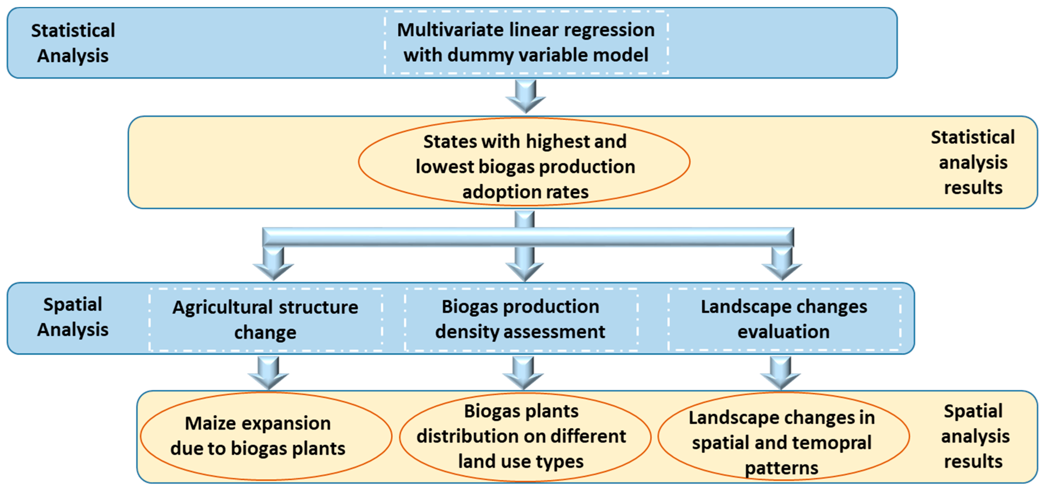
The main goal of this study was to identify the necessities of regional-based studies for German BPD analysis by answering the following research questions: (1) Is there state-level imbalanced BPD under the energy transition in Germany? (2) Are the environmental impacts of BPD distinguished between different levels of BPD? To study these two research questions, we adopted both empirical and spatial analyses. As the proxy of the state BPD, we used the BPAR in our study. By employing the multivariate linear regression with a dummy variable model (MLRDV), we accounted for the exogenous effects in the comparison among states. These effects were feedstock richness, production cost, and financial availability. On the basis of the empirical results, we identified the highest- and the lowest-BPAR states for further spatial analysis. The spatial analysis procedure was designed following the difference in difference (DiD) analysis approach [22]. By comparing the agricultural structural changes, biogas production densities, and the landscape changes of the selected states, we could clearly understand BPD’s impact on the environment, while accounting for other effects. If there are state-level imbalanced BPD and if a subsequent difference in the severity of environmental problems caused by BPD is detected, there would be a necessity to have more regional-based studies to study the BPD and the corresponding environmental problems in Germany. Figure 1 provides an overview of the research framework for this study.

2. Data and Methods

2.1. Data

We first collected the data for the empirical research on quantifying the German state-level BPAR. Three German city-states, i.e., Berlin, Bremen, and Hamburg, and the smallest federal state, Saarland, were excluded due to the data availability and quality. To control for the exogenous effects that might influence the BPAR of the studied states, the state-level data on various social–economic and agricultural factors of the studied states were gathered. In total, we collected the panel data for each of the studied 12 German federal states from 2000 to 2015.

Table 1. Description of collected data used in statistical analysis.

Variable	Abbreviation	Unit	Source
Installed capacity of each year newly established biogas plant	IC	kW/h	[23,24]
Yearly headcount of cattle	Cattle	head	[25]
Yearly headcount of pig	Pig	head	[25]
Yearly area of cultivated maize	Maize	ha	[25]
Yearly area of grassland	Grass	ha	[25]
Yearly per capita disposable income	DIC	Euro	[25]
Yearly average agricultural land transaction-based price	LP	Euro/ha	[25]
Yearly farming personnel	FP	-	[25]
Yearly utilized agricultural land	UTA	ha	[25]
Annual cattle manure electricity generation rate per head	$EG{R}_C$	kWh/head	[26]
Annual pig manure electricity generation rate per head	$EG{R}_P$	kWh/head	[26]
Annual maize electricity generation rate per hectare	$EG{R}_M$	kWh/ha	[26]
Annual grassland electricity generation rate per hectare	$EG{R}_G$	kWh/ha	[26]

presents the descriptive statistics of the collected data.

The spatial analysis aimed to quantify and compare the agricultural structure and landscape changes resulting from different BPD degrees during the studied period. Therefore, the data were collected at two time points, namely, before 2000 and after 2015, according to the data availability. In terms of agricultural structure change evaluation, we obtained the county-level data on silage maize cultivation area for the years 1999 and 2016 from the Federal Statistical Office of Germany. Moreover, we collected the Germany administrative unit spatial data at the NUT3 (Nomenclature of Territorial Units for Statistics) level. Regarding the biogas production density and landscape change evaluations, we made use of the Corine Land Cover (CLC) maps for the years 2000 and 2018. Furthermore, the geographical information on the biogas plants distribution and their corresponding installed capacity in Germany were extracted from EE-Monitor for the years 2000 and 2015. The EE-Monitor monitors the nature protection implications of the expansion of renewable energy in the power sector.

Table 2. Summary of the collected data for spatial analysis. NUTS, Nomenclature of Territorial Units for Statistics.

Data	Data Type	Time Range	Unit	Source
Biogas plant geographic information	Spatial	2000 to 2015	-	[23,24]
Silage maize cultivation area	Statistical	1999 and 2016	ha	[25]
Germany administrative area (NUTS3)	Spatial	2016	-	[27]
Corine Land Cover (CLC) map	Spatial	2000 and 2018	-	[28]

summarizes the collected data for spatial analysis.

2.2. Methods

2.2.1. Statistical Analysis

To empirically analyze the German state-level BPD, we made use of the MLRDV model to control for the exogenous effects. The MLRDV model could be dated back to 1950 [29]. From 1950 to 1980, this research method did not attract enough attention [30,31,32]. At the beginning of the 1980s, using the MLRDV model, Gibbons [33] proposed the basic methodology of event study, which focused on analyzing the impacts of policies and events. Since then, scholars have presented several examples of this approach and made this technique a well-known econometric technique [34,35,36,37,38]. As an extension of the univariate linear regression model, the MLRDV model allows studying the effect of the non-numeric independent variable by including it as a dummy variable in the regression model. The estimated coefficient on the dummy variable is interpreted as the independent effect of the underlying categorical variable on the dependent variable, after accounting for the effects of the other control variables in the model [39].

As the independent variable, we adopted the BPAR (ICPC) to proxy the state-level BPD. This variable was calculated by dividing the cumulative biogas plants installed capacity (IC) by the number of farming personnel (FP), which could also be regarded as state-level farmer per capita biogas plant installed capacity. Compared to the traditional indicators for bioenergy development, e.g., number of plants and total installed capacity, this variable further controlled for the state’s size effect to enable more appropriate comparisons among the states. The state detected to have higher BPAR was also more advanced in BPD. This variable was constructed as follows:

$$ICP{C}_t^i={{\displaystyle \sum }}_{j=0}^{t-2000}I{C}_{2000+j}^i/F{P}_t^i,$$

(1)

where t = 2000, 2001, …, 2015, and i = 12 studied German federal states.

Three variables were included as independent variables in the regression model to account for the effects that might influence the BPAR. The first one was the state-level biogas technical potential per hectare of utilized agricultural land, which was denoted as $BT{P}_t^i$. This variable indicated the richness of available biogas production feedstock, e.g., energy crops and manure, in the studied states. The biogas technical potential measured technical electricity productivity according to the availability of different feedstock types for biogas production [6,40,41,42]. As discussed in the previous research of Thiering [43], the transportation of substrates was inefficient from both economic and environmental perspectives. Therefore, the biomass for farm-scale biogas plants was generally obtained from a biogas plant’s immediate vicinity. This finding was confirmed by Csikos et al. [44], who found that biogas plants were concentrated in areas where energy crops were largely cultivated. In Germany, most of the biogas plants were medium-size farm-scale biogas plants [45]. Therefore, if the biogas technical potential per hectare of utilized agricultural land was high in a state, farmers from this state were prone to adopt biogas production. Furthermore, due to the varieties of Germany’s landscapes, the per hectare biogas technical potential varied enormously among the states during the studied period. Therefore, we included this variable in our regression model.

This variable was computed by calculating the state level biogas potential, which was proxied by the biogas-based electricity technical production volume using the available feedstock. In the current study, we adopted manure from cattle (Cattle) and pig (Pig), silage maize (Maize), and grass (Grass) as substrates for biogas production. After multiplying by the corresponding electricity generation rates (EGR_C, EGR_P, EGR_M, and EGR_G), the sum of the products was divided by the utilized agricultural lands of the states (UTA) to control for the state’s size effect.

$$BT{P}_t^i=\frac{Cattl{e}_t^i\times EG{R}_C+Pi{g}_t^i\times EG{R}_P+Maiz{e}_t^i\times EG{R}_M+Gras{s}_t^i\times EG{R}_G}{UT{A}_t^i},$$

(2)

where t = 2000, 2001, …, 2015, and i = 12 studied German federal states.

The second variable was the yearly state-level transaction-based average agriculture land price $L{P}_t^i$. The data on this variable were obtained directly from the Federal Statistical Office of Germany from 2000 to 2015. Arable land as a scarce production resource was needed for both building plants and providing feedstock for biogas production. Farmers only invested in a biogas plant if the production factors, e.g., farmland, were available or affordable [46]. Investors often leased or bought agricultural land for biogas production [47]. Under the EEG financing support, biogas production was more attractive than other traditional agricultural production activities. Farmers who wanted to build biogas plants but lacked land had a greater willingness to pay on the land market [48,49]. Consequently, the land purchase and rent prices were high in the regions where biogas production boomed [50,51,52,53]. However, as presented in the previous study, high agricultural land price might “scare away” the new biogas investors. Especially when the guaranteed subsidies of EEG were reduced, e.g., EEG 2014 emendation, the increasing land rental and purchase price would eat up the profit from biogas production investment [11]. Moreover, agricultural land prices also varied strongly among the federal states during the studied period. For example, in 2015, the transaction-based agricultural land price was 48,835 EUR/ha in Bavaria, while, in Thuringia, the price was only 10,450 EUR/ha.

The third variable was the federal state level yearly per capita disposal income $DI{C}_t^i$, which was used to control for the effect of regional economic situations and financial resources on answering EEG calls. As reported in other studies, more than half of the German agricultural biogas plants were in private hands [15]. Farmers who adopted the biogas plants anticipated this as an investment to diversify their income sources [43,54]. As reported by Rodriguez-Palenzuela and Dees [55], European savings and investing behaviors have been largely influenced by disposable income changes. The increase in disposable income generally led to a fall in savings and an increase in nominal consumption and investment. Therefore, disposable income played a vital role in the biogas plant adoption decision-making process. Additionally, the per capita disposable income increased significantly from 2000 to 2015, and much like the transaction-based agricultural land prices, the per capita disposable income varied strongly among the states. To control for this effect, the state-level disposable income per capita was taken into the regression model. The data on this variable were directly collected from the Federal Statistical Office of Germany.

Table 3. Descriptive statistics for selected variables used in statistical analysis.

Variables	Min	Mean	Median	Max	SD
ICPC (kW/h per capita)	0.0037	3.3953	2.4915	11.9663	3.2251
BTP (MW/h per ha)	2.79	5.27	5.20	8.23	1.37
LP (EUR per ha)	2460	13,906	12,366	48,835	9509
DIC (EUR per capita)	12,566	17,787	17,807	23,771	2603

shows the descriptive statistics of the selected variables.

After determining three control variables, the regression model was finally completed by including the state dummy variable $R{D}^i$ indicating the 12 studied federal states of Germany. To avoid the dummy variable trap, we coded 11 state categories for this dummy variable. The dropped state served as the reference in the result interpretation. The estimated coefficient on the dummy variable could be interpreted as the BPD of each studied state after controlling for the state’s size effect and other exogenous effects. The regression model was defined as follows:

$$ICP{C}_t^i=\alpha +BT{P}_t^i+ln(L{P}_t^i)+ln(DI{C}_t^i)+R{D}^i+{\epsilon }_t,$$

(3)

where t = 2000, 2001, …, 2015, and i = 12 studied German federal states.

2.2.2. Spatial Analysis

As Weiland [56] mentioned, maize as the primary biogas production feedstock was significantly more efficient than manure. Consequently, a large segment of biogas plants were running on energy crops, with silage maize representing about 70% of the biogas input for energy crops and contributing around 56% of the total biogas energy production [5,57,58]. Dornburg [59] generally discussed the conflicts between the increasing demand for biogas and biodiversity, water availability, and food security. Gawel and Ludwig [60] pointed out a prevailing structural change in agricultural production during the EEG period. This agricultural structure change is also known as the “maizification” and has led to significant changes in agricultural land use [61]. Scholars argued that the expansion of silage maize was at the cost of losing land use for food production, which raised the agricultural land price and threatened food security [47,62,63]. Furthermore, Hötker et al. [64] argued that maize cultivation was intensive and included more fertilizer and pesticides than other crops. The intensification of energy crop cultivation also led to a loss of crop diversity, negative influence on soil fertility, and reduction in farmland biodiversity [65,66,67]. Furthermore, to realize the economies of scale, biogas plant operators were prone to have larger plants. The high feedstock demand of large-size plants might cause indirect land-use change (iLUC) and greenhouse gas (GHG) emissions during the feedstock transportation [11,60].

Against this background, the current study focused on determining the impacts of BPD on the environment, namely, the assessments of agricultural structural change, biogas production density, and landscape pattern change. The spatial analysis procedure followed the DiD research design by spatially comparing the changes in the three abovementioned aspects between states with the highest and the lowest BPARs over the studied period. This research procedure allowed us to identify the influences on the environment of different BPD levels and conclude that the detected difference in the influence was a consequence of BPD.

The first spatial analysis focus was on the agricultural production structural change caused by maize expansion. We first computed the silage maize cultivation area of 1999 and 2016 for each county in Germany. Then, we calculated the growth rate of the maize cultivation areas during this period. The calculated county-level growth rate of maize cultivation area was further spatialized at the NUT3 level by using ArcGIS. To determine whether the silage maize expansion was accompanied by the bioenergy development, we further spatially compared the county-level maize expansion rates between the highest- and the lowest-BPAR states.

The focus of the second spatial analysis was on the biogas production density on different land-use types. We first used the CLC inventory data in 2000 and 2018 to assess the regional land-use change during the studied period. The land-use types were aggregated into eight categories, which are summarized in

Table 4. Land-use types in the current study.

Land Use Types	Abbreviation	CLC Code	Specification
Urban areas	UA	111	Continuous urban fabric
		112	Discontinuous urban fabric
		121	Industrial or commercial units
		122	Road and rail networks and associated land
		123	Port areas
		124	Airports
		131	Mineral extraction sites
		132	Dump sites
		133	Construction sites
		141	Green urban areas
		142	Sport and leisure facilities
Arable land	AL	211	Non-irrigated arable land
Pastures	PA	231	Pastures
Other agriculture land	OA	221	Permanently irrigated land
		222	Rice fields
		242	Complex cultivation patterns
		243	Land principally occupied by agriculture, with significant areas of natural vegetation
Forests	FO	311	Broad-leaved forest
		312	Coniferous forest
		313	Mixed forest
Natural grassland	NG	321	Natural grasslands
Other vegetated land	OV	322	Moors and heathland
		324	Transitional woodland shrub
		331	Beaches, dunes, sands
		333	Sparsely vegetated areas
		334	Burnt areas
Wetlands and waterbodies	WW	411	Inland marshes
		412	Peat bogs
		421	Salt marshes
		422	Salines
		511	Water courses
		512	Water bodies
		521	Coastal lagoons
		522	Estuaries

Source: Corine Land Cover change maps, European Environment Agency.

. After this, the spatial distribution map of biogas plants was overlaid with the CLC 2018 map to identify the densities of biogas plants on different land-use types. Then, we compared the average installed capacity between the selected states on each land-use type. Moreover, the proportions of installed capacity and number of biogas plants on each land-use type of the total state installed capacity and the number of biogas plants were calculated.

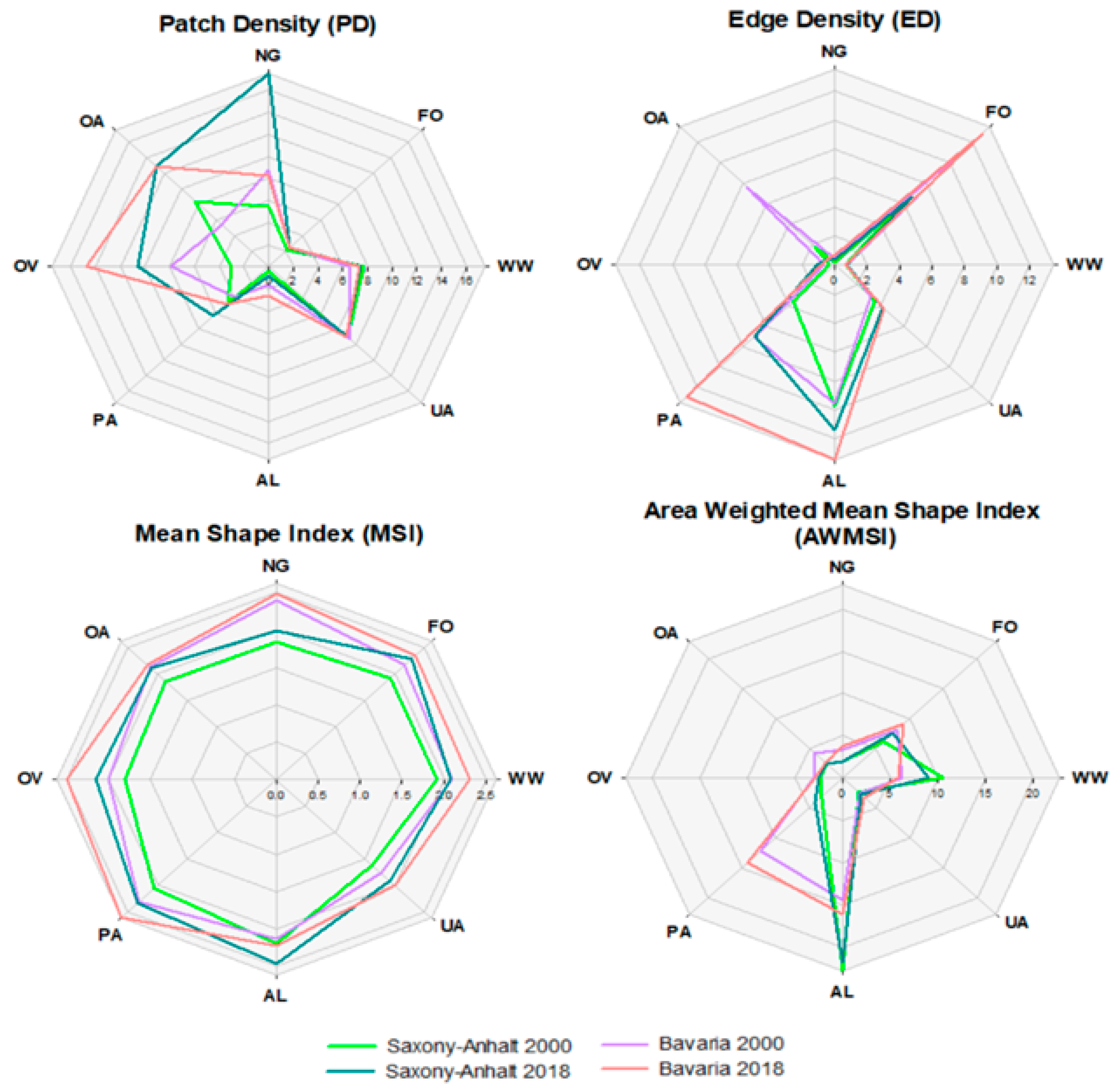
The third aspect was quantifying the spatial and temporal patterns changes of landscape in the selected federal states using the landscape matrices, which were calculated using the ArcGIS extension package Patch Analyst 5.1. This approach contained nonspatial composition analysis, e.g., abundance of patch types, and spatial configuration analysis, e.g., patch shape, to understand the spatial heterogeneity and fragmentation of the natural ecosystems. The CLC map 2000 and CLC map 2018 in vector format were used to conduct the patch analysis. Seven matrices were considered in this research: (1) class area (CA), (2) number of patches (NumP), (3) mean patch size (MPS), (4) mean shape index (MSI), (5) area-weighted mean shape index (AWMSI), (6) edge density (ED), and (7) patch density (PD). CA and NumP were the indicators illustrating the landscape change process of the state. MPS was the primary predictor of diversity within a patch. MSI and AWMSI could be used to assess patch diversity and sensitivity to fragmentation. ED was related to the degree of spatial heterogeneity and was used to describe the dynamics of the abundances and attributes of specific types of edges. PD was a limited, but fundamental index of landscape pattern analysis. Compared to NumP, this index further expressed the number of patches on a per unit area basis that could facilitate the comparisons among landscapes of various sizes.

Table 5. Landscape matrix indicator calculation.

Metric	Calculation	Unit	Specification
Class area (CA)	${{\displaystyle \sum }}_{j=1}^n{a}_{ij}/A$	ha	Where aij is the area (m2) of patch j for the i-th land-use type, and A is the total landscape area (m2).
Number of patches (NumP)	${{\displaystyle \sum }}_{i=1}^n{P}_i$	number	Where Pi refers to the number of patches of type i.
Mean patch size (MPS)	${{\displaystyle \sum }}_{i=1}^n{a}_i/m$	ha	Where ai is the patch size, and m is the total patch number of the i-th landscape.
Mean shape index (MSI)	${{\displaystyle \sum }}_{j=1}^n\left(\frac{P_{ij}}{\sqrt[2]{\pi \ast a_{ij}}}\right)/n_i$	-	Where Pij is the perimeter of patch ij, and ni is the number of patches of the same type.
Area-weighted mean shape index (AWMSI)	${{\displaystyle \sum }}_{j=1}^n\left[\frac{P_{ij}}{min{P}_{ij}}\left(\frac{a_{ij}}{{{\displaystyle \sum }}_{j=1}^n{a}_{ij}}\right)\right]$	-	Where minPij is the minimum perimeter of patch ij in terms of number of cell edges.
Edge density (ED)	$TE/TLA$	m/ha	Where TE is the total edge, which is defined as the length of edge that exists at the interface between two classes, and TLA is the total landscape area.
Patch density (PD)	${{\displaystyle \sum }}_{i=1}^{n}Pi/TLA$	number/100 ha	Where Pi refers to the number of patches of type i.

provides detailed equations and explanations of these landscape matrices.

3. Results

3.1. State-Level Bioenergy Production Development

To avoid the dummy variable trap, we randomly dropped the federal state Hesse in the region dummy variable categories. The regression results are summarized in

Table 6. Regression results.

Variables	Coefficient	Standard Error	t-Value
Intercept	−155.46 ***	8.64	−17.76
Control Variables
BTP	3.52 ***	0.27	13.07
ln(LP)	12.18 ***	1.06	11.52
ln(DIC)	1.68 ***	0.30	5.59
Region Dummy Variables
Schleswig-Holstein	−3.78 ***	0.56	−6.57
Lower Saxony	−0.77	0.48	−1.61
North Rhine-Westphalia	−2.64 ***	0.37	−7.17
Rhineland-Palatinate	1.95 ***	0.29	6.68
Baden-Württemberg	−2.99 ***	0.30	−9.80
Bavaria	−5.22 ***	0.40	−12.94
Brandenburg	8.66 ***	0.33	26.44
Mecklenburg-Vorpommern	12.83 ***	0.35	36.65
Saxony	8.89 ***	0.34	26.53
Saxony-Anhalt	14.46 ***	0.50	29.03
Thuringia	10.52 ***	0.36	29.63
Adjusted R2	0.95
Sample size	192

Note: *** denotes 99.9% confidence level.

. The variance inflation factor test was adopted to test the multicollinearity of the independent variables in the regression. The result is reported in Table S1 (Supplementary Materials). In addition, the normality of the regression residuals was checked using Shapiro–Wilk and Kolmogorov–Smirnov tests. The result is presented in Table S2 (Supplementary Materials). The linear regression model diagnostic plots for residuals can be found in Figure S1 (Supplementary Materials).

As shown in Table 6, there were significant variations in state-level BPAR after controlling for the other exogenous effects. Moreover, the control variables were all highly significant, suggesting their substantial impact on BPAR. Compared to Hesse, Saxony-Anhalt and Mecklenburg-Vorpommern had, on average, 14.46 and 12.83 kW/h more per capita biogas plants installed capacity during the studied period from 2000 to 2015, whereas Bavaria and Baden-Württemberg had per capita 5.22 and 2.99 kW/h less, after controlling for all other effects. In general, we found that the federal states in former East Germany had comparably higher BPAR than the states in former West Germany. Saxony-Anhalt was the state with the highest BPAR among all the studied 12 federal states in Germany, while Bavaria’s BPAR was the lowest. All these findings implicated that, under the nationwide unified EEG financial support, states had different BPARs, indicating the imbalanced BPD of Germany federal state during the studied EEG period.

3.2. Agricultural Structural Change

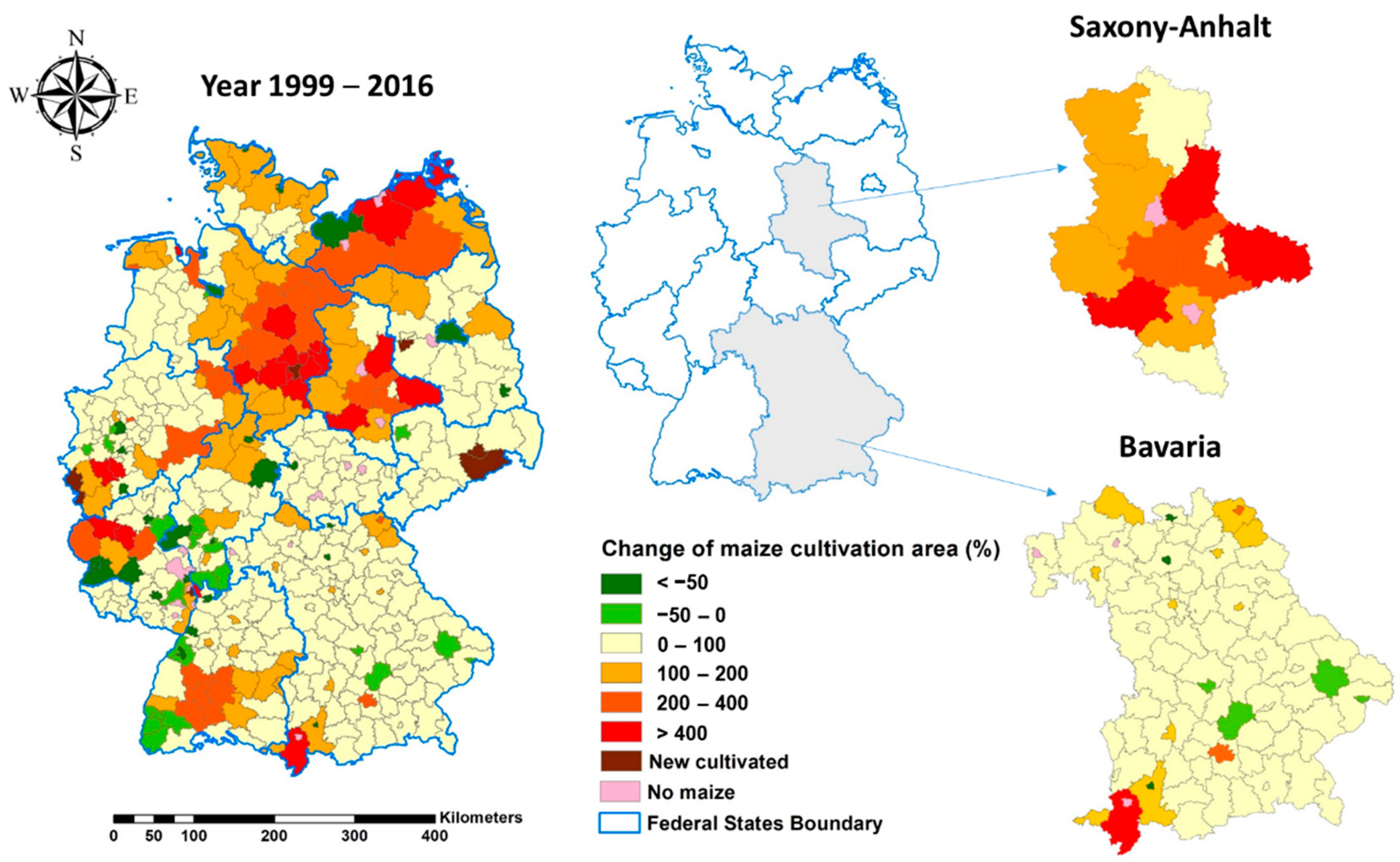
The large spatial discrepancy of maize expansion rates among all the studied German counties is displayed in Figure 2. As shown, Germany experienced a substantial maize expansion from 1999 to 2016. Over 330 counties reported an increasing maize cultivation area with the growth rates varying from 0.21% to 2851.72%. Furthermore, six counties were starting to practice silage maize cultivation during this period. In contrast, the maize cultivation area decreased in only 24 counties, and 23 counties remained with no maize cultivation.

Compared to 1999, the average silage maize cultivation area in Saxony-Anhalt and Bavaria in 2016 increased by 229.04% and 65.36%, respectively. Specifically, the county-level maize expansion of these two states showed large variations. For instance, 71% of the Saxony-Anhalt counties had increased maize cultivation area from 1999 to 2016 with the growth rates varying between 52.09% and 776.54%. In contrast, Bavaria showed a milder change among the counties. About 88% of the Bavaria counties observed an increasing maize cultivation area with the maize cultivation area’s growth rates in a lower and narrower range from 0.42% to 340.83%. Around 7% of Bavaria counties even showed decreased maize cultivation or became no-maize counties during this period.

3.3. Biogas Production Density on Various Land-Use Types

As reported in

Table 7. Land-use change patterns in Saxony-Anhalt and Bavaria from 2000 to 2018.

Land-Use Types	Percentage of Landscape (%)				Percentage Change 2000–2018 (%)		Absolute Area Change 2000–2018 (%)
	SA_00	SA_18	BA_00	BA_18	SA	BA	SA	BA
UR	7.20	7.18	5.65	6.92	−0.01	1.27	−0.18	22.46
AL	58.45	54.86	29.23	33.4	−3.59	4.16	−6.15	14.24
PA	7.51	11.48	13.55	20.26	3.97	6.71	52.81	49.53
OA	2.83	0.76	13.86	0.82	−2.07	−13.04	−73.10	−94.05
FO	21.33	22.61	34.28	35.32	1.28	1.04	6.00	3.03
NG	0.55	0.31	0.79	1.06	−0.18	0.27	−32.26	34.71
OV	1.30	1.64	1.40	1.11	0.33	−0.29	25.46	−20.97
WW	0.82	1.10	1.23	1.11	0.28	0.13	33.62	−10.33

Note: SA: Saxony-Anhalt, BA: Bavaria, UR: urban area, AL: arable land, OA: other agricultural area, FO: forests, NG: natural grassland, OV: other vegetated land, WW: wetland and waterbodies.

, the dominant land-use type in Saxony-Anhalt was arable land, which occupied more than half of the landscape. Forest land was the second-largest land-use type in Saxony-Anhalt. In Bavaria, the dominant land-use types were also the arable land and forest, which had similar proportions. The proportion of other agricultural area showed a decreasing trend in both states from 2000 to 2018, with a larger decline being observed in Bavaria. This mainly resulted from the conversion to arable land and pasture to fulfill the land requirement for bioenergy and food crop cultivation, as well as regional animal farming business development. The change matrices are summarized in Tables S3 and S4 (Supplementary Materials).

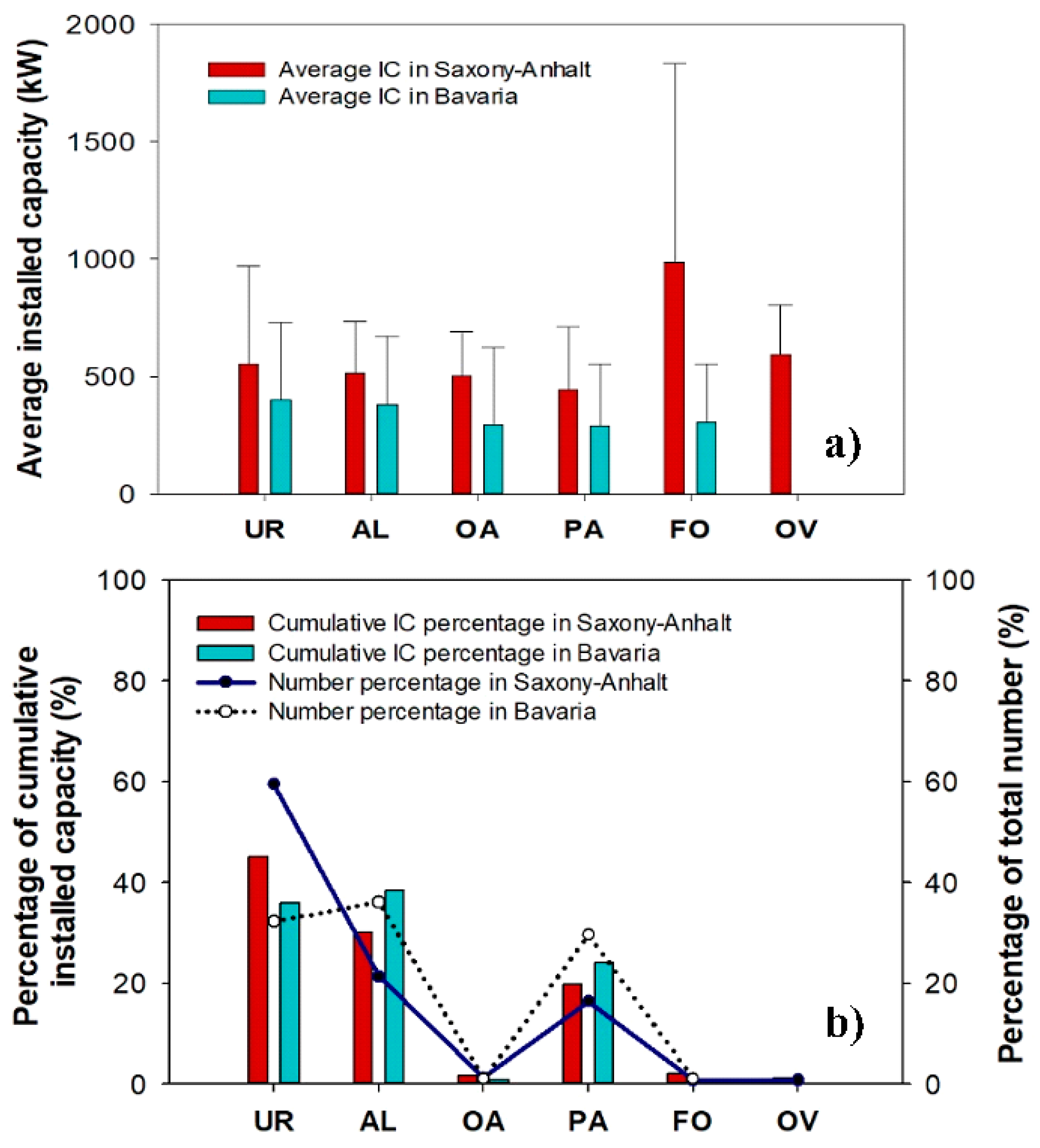
As shown in Figure 3a, Saxony-Anhalt demonstrated a bigger average biogas plant size on all the studied land-use types than Bavaria. The average biogas plant installed capacity ranged from 291.03 to 398.06 kW/h on the six studied land-use types in Bavaria, whereas the mean size of plants ranged from 442.84 to 984.33 kW/h on these six types in Saxony-Anhalt. The largest average plant size was 984 kW/h, which was found in forests in Saxony-Anhalt. This was three times bigger than the average plant size located in Bavaria forests. The mean size of biogas plants located in other vegetated areas in Saxony-Anhalt was 593 kW/h, and no biogas plant was found on this land-use type in Bavaria. Generally, Bavaria displayed a biogas production system dominated by small-scale plants, while the plants in Saxony-Anhalt were relatively large.

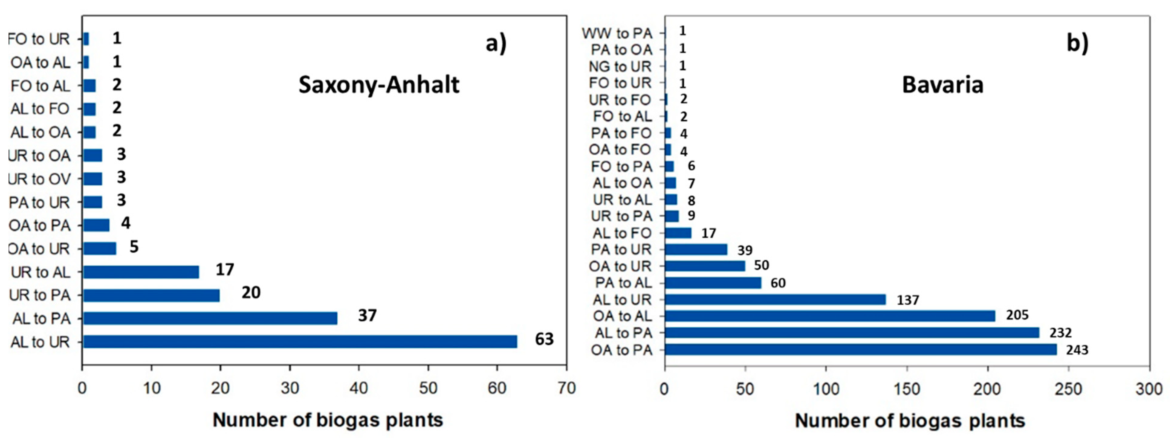
In Saxony-Anhalt and Bavaria, the number of biogas plants increased from three to 403 and from 80 to 2848, and the cumulative installed capacity raised from 2211 to 213,754 kW/h and from 16,018 to 1,019,751 kW/h during the period through 2000 to 2015, respectively. As presented in Figure 3b, according to the CLC 2018, a large number of established biogas plants until 2015 were distributed in the urban area, arable land, and pastures in both states. Compared to Bavaria where the biogas production was more evenly distributed in these three land-use types, Saxony-Anhalt had a significantly larger proportion of biogas plants built in the current urban area, with a corresponding higher total installed capacity. However, it should be mentioned that both states experienced intense land-use change from 2000 to 2018. Biogas plants located in the urban area according to CLC 2018 might have been built at that time in another land-use type. Figure 4 summarizes the changes in all land-use types on which the biogas plants were built until 2015 according to the comparison between CLC 2000 and CLC 2018. As shown, the biogas plants distributed on land-use types such as urban area and forest were originally converted from other land-use types, e.g., arable land or other vegetated area.

3.4. Landscape Pattern Change

The fragmentation of a certain land-use type was detected, if an increase in patch number and a decline in patch size of this land-use type were observed simultaneously. As reported in Panel A of

Table 8. The patch number and mean patch size in various land-use classes.

Land Use Types	Number of Patches (MumP)			Mean Patch Size (MPS)
	2000	2018	Change	2000	2018	Change
Panel A: Saxony-Anhalt
UR	1349.00	1315.00	−2.52%	109.65	112.29	2.40%
AL	483.00	978.00	102.48%	2487.51	1152.94	−53.65%
PA	718.00	1481.00	106.27%	215.06	159.32	−25.92%
OA	490.00	202.00	−58.78%	118.83	77.52	−34.76%
FO	953.00	1147.00	20.36%	459.93	405.08	−11.93%
NG	62.00	134.00	116.13%	182.37	57.16	−68.66%
OV	80.00	357.00	346.25%	335.19	94.24	−71.88%
WW	130.00	169.00	30.00%	130.17	133.79	2.78%
Panel B: Bavaria
UR	3735.00	4370.00	17.00%	106.70	111.68	4.67%
AL	3494.00	6284.00	79.85%	590.29	374.98	−36.48%
PA	3698.00	6905.00	86.72%	258.45	206.99	−19.91%
OA	5278.00	750.00	−85.79%	185.25	77.59	−58.11%
FO	5773.00	5986.00	3.69%	418.94	416.35	−0.62%
NG	489.00	620.00	26.79%	113.70	120.79	6.23%
OV	777.00	1155.00	48.65%	127.26	67.67	−46.82%
WW	564.00	571.00	1.24%	154.22	136.63	−11.41%

Note: SA: Saxony-Anhalt, BA: Bavaria, UR: urban area, AL: arable land, OA: other agricultural area, FO: forests, NG: natural grassland, OV: other vegetated land, WW: wetland and waterbodies.

, in Saxony-Anhalt, an increase in the number of patches was observed in almost all land-use types from 2000 to 2018 with the exception of other vegetated area and urban area. The most substantial increase in patch number was found in other vegetated areas with an increment of 346.25%, followed by natural grasslands, pastures, and arable land. As to the mean patch size change, sharp decreases were observed in the other vegetated area (−71.88%), natural grasslands, arable land, and other agricultural land. These observations indicated that other vegetated area, natural grasslands, and arable land in Saxony-Anhalt experienced stronger fragmentation. In terms of Bavaria, the results are summarized in Panel B of Table 8. The strongest rise in the number of patches was detected in pastures with an increase of 86.72%, followed by arable land and other vegetated land. The decreases in the mean patch size were mainly identified in other agricultural land, other vegetated land, and arable land in Bavaria. Forest, as an important flora and fauna habitat, increased in both Saxony-Anhalt and Bavaria from 2000 to 2018. In Saxony-Anhalt, the number of patches increased by 20.36% and the mean patch size decreased by 11.93%, while, in Bavaria, the number of patches showed a slight increase of 3.69% and the change in mean patch size was negligible.

According to Figure 5, both Saxony-Anhalt and Bavaria showed increased PD from 2000 to 2018. The highest PD was found in natural grassland in Saxony-Anhalt and in other vegetated land in Bavaria. The change in ED suggested a higher degree of spatial heterogeneity and types of edges in Bavaria than in Saxony-Anhalt. This could especially be observed in the land-use classes of forest land, arable land, and pastures. These findings indicated that the patches in other agricultural land became smaller and more compact in both states. However, this was accompanied by a rapid decrease in edge types and spatial heterogeneity. MSI showed an upward trend in both federal states. Specifically, except for arable land, Bavaria showed a higher level of patch diversity than Saxony-Anhalt in all the land-use classes. The AWMSI analyzed the perimeter–area relationship of the patches. The result showed that the arable land in Saxony-Anhalt, as well as the arable land and pastures in Bavaria, were clearly more sensitive to fragmentation than any other land-use types.

4. Discussion

After controlling for the exogenous environmental and economic effects, the empirical results indicated that the BPARs varied enormously among the studied German federal states. Since the EEG promotion program was unified at the national level, the variations in state-level BPAR could be due to differences in state-level promotion programs, such as Energie und Klimaschutz in Saxony, Energie in Saxony-Anhalt, and Bioenergiewettbewerb in Baden-Württemberg or farmers’ personality traits and risk cognitions [68]. In this section, we focus on discussing the farmers’ personality traits and investment risk cognitions and their biogas production adoption behaviors.

For many farmers in Germany, operating biogas plants was an alternative investment to diversify their income sources [5,43,54]. Under the same investment conditions and returns provided by EEG, it was clear that farmers from different states anticipated this investment differently. As reported in previous studies, there existed a correlation of attitudes toward behavior [69,70]. Therefore, the variations in attitudes toward bioenergy production investment led to farmers’ heterogeneous behaviors. Since, in the regression model, the exogenous effects that objectively influence the biogas production adoption were controlled for, the variations in behaviors resulted from the differences in farmers’ endogenous factors that influenced the investment decision subjectively. Studied systematically in behavior finance, these factors were the investors’ personality traits and risk cognitions, such as time preference, risk preference, and perception [69,71,72,73].

As found by Liu [74], more risk-averse farmers needed significantly more time to adopt a new form of agricultural biotechnology. Moreover, in Germany, a large number of biogas plants were operated in private hands [15]. Local farmers needed credit to facilitate the construction of biogas plants [75]. As discussed in Brown et al. [76], more risk-averse households were less tolerant of fluctuations in their financial circumstances and, therefore, were less prone to take debt. Daly et al. [77] also argued a positive linear relationship between the probability of applying loans and the risk attitude. Therefore, despite the availability of low-interest biogas plant construction loans, risk-averse farmers might still resist holding debt to build biogas plants [78]. Furthermore, as demonstrated by Wang et al. [73], the responses to the “wait-or-not” question ($3400 this month or $3800 next month) were highly heterogeneous among a large segment of the population in the world. Even inside Germany, there was a difference in time preference between the residents of former East and West Germany [79]. These findings indicated that people’s activities varied in terms of their orientation toward the present or toward the future. Due to the loan repayments, the farmers’ annual income might be even lower than before when operating biogas plant in the first few years. After paying back all the debts, much higher profits could be obtained by the operators. Thus, risk-neutral but less patient farmers might refuse to adopt biogas plants. However, to have a more conclusive argument, a further regional study is needed.

To raise the BPAR, the EEG’s remuneration is to be increased to attract the farmers who are comparably reluctant to build biogas plants. However, since the EEG subsidy scheme is nationwide unified, the increase in remuneration might lead to overreaction in states where farmers are willing to operate biogas plants for even lower subsidy. In the current study, we already observed significant state-level differences in adopting biogas production. A further increase in the subsidy to promote biogas adoption in states such as Bavaria and Baden-Württemberg might lead to overreactions in, for instance, Saxony-Anhalt and Mecklenburg-Vorpommern.

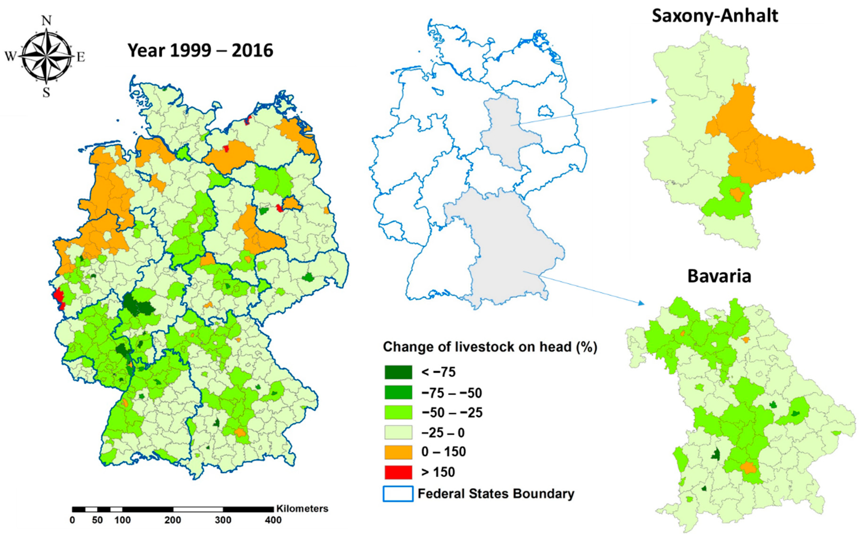
Compared to Bavaria, Saxony-Anhalt with a much higher BPAR was more vulnerable to biogas production-related agricultural and environmental problems. For instance, we observed stronger agricultural production structure change reflecting in maizification in Saxony-Anhalt than in Bavaria. Since we could not distinguish the purposes of the cultivated silage maize between the feed for livestock and the substrate for biogas production, the expansion of the total silage maize cultivated area could also be induced by the development of livestock farming. Figure 6 presents the livestock unit change (German: Großvieheinheit) on hand in Germany between 1999 and 2016. Generally, Germany showed a decline in livestock on hand during this period, with approximately 88% of counties in Germany having a negative growth rate. Compared to Bavaria, where only 3% of counties had an increase in livestock unit on hand, 43% of counties from Saxony-Anhalt showed expansion of livestock farming from 1999 to 2016. The decrease rates in livestock unit on hand of the counties in Saxony-Anhalt were normally no less than −25%, whereas, in Bavaria, these rates were down to −50%. In summary, both states experienced a decline in livestock farming; while, in Bavaria, the livestock units on hand declined by more than 18%, Saxony-Anhalt had a relatively flat downward trend with the decrease rate being less than 8% during the period 1999 to 2016. As shown in Figure 7, the nationwide cultivation area of silage maize used for livestock farming also decreased from 2007 to 2015, while the cultivation area of silage maize for biogas production strongly increased in these 9 years [80]. Therefore, we could draw a preliminary conclusion that the observed substantial maize expansion in Saxony-Anhalt was mainly due to the rapid development of biogas production.

The increased land use for maize production crowded out the local food and cultural crop cultivation [46,47,62,63]. Moreover, the environmental impacts of biogas plants were attributed mainly to energy crop production from the life-cycle perspective. The results of a regional life cycle assessment (RELCA) model showed that the feedstock cultivation contributed about 52–67% of the total GHG emissions for biogas production in Central Germany [81,82]. Compared to a fossil-fuel-based system for electricity and heat supply, it appeared that specific eutrophication and acidification potentials for biogas from maize were significantly higher [15].

The biogas production density analysis indicated that the biogas production was more concentrated in urban areas than in other land-use types in Saxony-Anhalt. According to Daniel-Gromke et al. [20], about 92.60% of the total input for biogas production in Germany was energy crops and animal excrement. In Saxony-Anhalt, only 15 biogas plants were biowaste digestion plants until 2016 [83]. Therefore, only a small proportion of plants located in urban areas ran on household and industrial wastes. The operation of other urban-located plants relied on energy crops and manure, which needed to be transported from arable land. We further observed that most of the biogas plants in Bavaria were small-scale, while the plants’ installed capacity in Saxony-Anhalt was generally large. This might be because about 49% of Saxony-Anhalt farms were larger than 100 ha, while only 4% of farms in Bavaria reached this scale. Around 50% of the farms in Bavaria were less than 20 ha [84]. The high demand for transported feedstock in Saxony-Anhalt raised the cautions of the potential iLUC risks and GHG emissions. Additionally, agricultural biogas plants in the urban area might also influence the city and town dwelling life quality. As argued by Paterson et al. [85], many residents resist the biogas production under the motto “not in my backyard” because biogas plants are smelly and plant operation brings a risk of explosion.

The land change analysis results suggested high fragmentation of arable land and pastures in both states from 2000 to 2018. One of the driving factors was the intensified animal farming and energy crop cultivation during the EEG period. This was consistent with Csikos et al. [44], who detected changes in landscape patterns, reduced crop diversity, and the homogenization of arable land and pastures, after introducing biogas plants. However, compared to Bavaria, Saxony-Anhalt with more rapid biogas production development showed lower landscape heterogeneity and higher vulnerability to fragmentation. Regarding the forest, Campbell and Doswald [86] and Hartmann [87] reported a negative relationship between biogas production development and species biodiversity due to loss of habitat. In the current study, although there was no severe fragmentation detected in both states, the forest in Saxony-Anhalt showed a relatively strong increase in the number of patches and a decrease in the mean patch size. This observation also indicated a potential threat of biogas production to species habitat and regional biodiversity.

5. Conclusions and Outlook

This study contributed to the current literature of biogas production development under Germany’s energy transition by comparing the German state-level biogas production development during the studied period from 2000 to 2015, after accounting for the exogenous effects. We identified that there were uneven developments of biogas production among the federal states in Germany. Moreover, unlike most other studies that claimed Bavaria and Lower Saxony were the leading states in biogas production development, we found that the per capita biogas plant installed capacity in the former East Germany states was significantly higher. Apart from other reasons such as scales of farms, development of livestock farming, and state-level support, this could be due to the diversities of farmers’ personality traits and risk cognitions, which led to different attitudes toward the biogas production investment. Furthermore, in the spatial analysis, we identified that the biogas production-related environmental problems in the states with higher per capita biogas plant installed capacity were more severe. For instance, stronger maize expansion was observed in the region with higher BPAR. Additionally, we observed that more biogas plants in the state with higher BPAR were located in nonarable areas, which could result in iLUC and higher GHG emissions during feedstock transportation. Furthermore, we also found that fragmentation of arable land and pastures accompanied the biogas development. Higher-BPAR regions were more vulnerable to habitat and regional biodiversity losses. Therefore, to increase the BPAR in the states where the farmers responded to the EEG weakly, an increase in the nationwide unified subsidy might lead to an overreaction of those strong response states. The overreactions could lead to severe agricultural and environmental problems identified in this research.

The presented study also had limitations due to data availability. Firstly, we could not obtain the data about the feedstock types of each biogas plant. Moreover, as mentioned in the discussion, in the regional crop statistic record, the cultivated silage maize’s usage was not differentiated between biogas production feedstock and livestock fodder. We surveyed the published literature and found that the Integrated Administration and Control System (IACS) could be a very crucial data source for similar research. This information system could provide spatially and temporally precise information on agricultural land use, and it classifies the total silage maize area into different groups according to their utilization [4].

The current study results emphasized the necessity of future regional-based studies to support more sustainable bioenergy management under the German energy transition. For instance, to sustainably develop the national level biogas production and avoid overreaction of some states, future studies should focus on the states where farmers are less willing to adopt biogas production. Therefore, a more regional-based behavior finance study supported by local survey data could help to understand the farmers’ concerns in adopting biogas plants and could provide the solution to increasing the BPAR of these states or regions. Furthermore, to study the impacts caused by biogas production development, more regional-based studies are required to cope with the regional heterogeneities in the future. Some well-developed approaches can be found in the literature. For instance, to evaluate the environmental burdens associated with the bioenergy production value chain, regional-based LCA is more applicable. One of the regional-based LCA models is the RELCA model [82], which can capture site-specific characteristics and enable a reliable and accurate environmental impact assessment. In terms of the social impact of bioenergy production, the regional specific contextualized social life cycle assessment model (RESPONSA) [88,89] could be applied.

References

- Quitzow, L.; Canzler, W.; Grundmann, P.; Leibenath, M.; Moss, T.; Rave, T. The German energiewende–What’s happening? Introducing the special issue. Util. Policy 2016, 41, 163–171. [Google Scholar] [CrossRef]
- Laird, F.N.; Stefes, C. The diverging paths of German and United States policies for renewable energy: Sources of difference. Energy Policy 2009, 37, 2619–2629. [Google Scholar] [CrossRef]
- Sims, R.E.H.; Hastings, A.; Schlamadinger, B.; Taylor, G.; Smith, P. Energy crops: Current status and future prospects. Glob. Change Biol. 2006, 12, 2054–2076. [Google Scholar] [CrossRef]
- Vergara, F.; Lakes, T. Maizification of the Landscape for Biogas Production? Identifying the likelihood of Silage Maize for Biogas in Brandenburg from 2008–2018; Open-Access-Publikationsserver der Humboldt-Universität: Berlin, Germany, 2019. [Google Scholar]
- Grundmann, P.; Ehlers, M.-H.; Uckert, G. Responses of agricultural bioenergy sectors in Brandenburg (Germany) to climate, economic and legal changes: An application of Holling’s adaptive cycle. Energy Policy 2012, 48, 118–129. [Google Scholar] [CrossRef]
- Budzianowski, W.M.; Chasiak, I. The expansion of biogas fuelled power plants in Germany during the 2001–2010 decade: Main sustainable conclusions for Poland. J. Power Technol. 2011, 91, 102–113. [Google Scholar]
- Daniel-Gromke, J.; Rensberg, N.; Denysenko, V.; Trommler, M.; Reinholz, T.; Völler, K.; Beil, M.; Beyrich, W. Anlagenbestand Biogas und Biomethan–Biogaserzeugung und -Nutzung in Deutschland(DBFZ Report Nr. 30); Deutsches Biomasseforschungszentrum Gemeinnützige GmbH (DBFZ): Leipzig, Germany, 2017. [Google Scholar]
- Rensberg, N.; Schumacher, B.; Liebetrau, J. Verfügbare ungenutzter Substratpotenziale und Hemmnisse bei deren energetischer Nutzung in Deutschland; Deutsches Biomasseforschungszentrum Gemeinnützige GmbH (DBFZ): Leipzig, Germany, 2019. [Google Scholar]
- FNR. Bioenergy in Germany Acts and Figures; Agency for Renewable Resources: Gülzow-Prüzen, Germany, 2019.
- Thrän, D.; Schaubach, K.; Majer, S.; Horschig, T. Governance of sustainability in the German biogas sector—Adaptive management of the renewable energy act between agriculture and the energy sector. Energy Sustain. Soc. 2020, 10, 1–18. [Google Scholar] [CrossRef]
- Appel, F.; Ostermeyer-Wiethaup, A.; Balmann, A. Effects of the German renewable energy act on structural change in agriculture–The case of biogas. Util. Policy 2016, 41, 172–182. [Google Scholar] [CrossRef]
- Purkus, A.; Gawel, E.; Szarka, N.; Lauer, M.; Lenz, V.; Ortwein, A.; Tafarte, P.; Eichhorn, M.; Thrän, D. Contributions of flexible power generation from biomass to a secure and cost-effective electricity supply—A review of potentials, incentives and obstacles in Germany. Energ. Sustain. Soc. 2018, 8, 1–21. [Google Scholar] [CrossRef]
- Torrijos, M. State of development of biogas production in Europe. Procedia Environ. Sci. 2016, 35, 881–889. [Google Scholar] [CrossRef]
- Scarlat, N.; Dallemand, J.-F.; Fahl, F. Biogas: Developments and perspectives in Europe. Renew. Energy 2018, 129, 457–472. [Google Scholar] [CrossRef]
- Lebuhn, M.; Munk, B.; Effenberger, M. Agricultural biogas production in Germany–From practice to microbiology basics. Energy Sustain. Soc. 2014, 4, 1–21. [Google Scholar] [CrossRef] [Green Version]
- DBFZ. Nachhaltige Biogaserzeugung in Deutschland–Bewertung der Wirkungen des EEG; Deutsches Biomasseforschungszentrum Gemeinnützige GmbH (DBFZ): Leipzig, Germany, 2011. [Google Scholar]
- Niedersachsen-Netzwerk, N.R.V. Biogas in Lower Saxony; 3N Centre of Experts for Renewable Resources Lower Saxony: Werlte, Germany, 2014. [Google Scholar]
- Diekmann, J.; Schill, W.-P.; Vogel-Sperl, A.; Püttner, A.; Schmidt, J.; Kirrmann, S. Vergleich der Bundesländer: Analyse der Erfolgsfaktoren für den Ausbau der Erneuerbaren Energien 2014–Indikatoren und Ranking; DIW: Berlin, Germany; ZSW: Stuttgart, Germany; Agentur für Erneuerbare Energien e.V.: Berlin, Germany, 2014. [Google Scholar]
- Strommix und Anteile Erneuerbarer Energien in den Bundesländern 2013. Available online: https://www.unendlich-viel-energie.de/erneuerbare-energie/wasser/strommix-und-anteile-erneuerbarer-energien-in-den-bundeslaendern (accessed on 20 March 2020).
- Daniel-Gromke, J.; Rensberg, N.; Denysenko, V.; Stinner, W.; Schmalfuß, T.; Scheftelowitz, M.; Nelles, M.; Liebetrau, J. Current developments in production and utilization of biogas and biomethane in Germany. Chem. Ing. Tech. 2018, 90, 17–35. [Google Scholar] [CrossRef]
- Majer, S.; Stecher, K.; Adler, P.; Daniel, T.; Müller-Langer, F. Biomass Potentials and Competition for Biomass Utilisation; Deutsches Zentrum für Luft- und Raumfahrt e.V, DLR: Stuttgart, Germany, 2013. [Google Scholar]
- Lechner, M. The estimation of causal effects by difference-in-difference methods estimation of spatial panels. Found. Trends Econ. 2010, 4, 165–224. [Google Scholar] [CrossRef] [Green Version]
- EE-Monitor POF3–Y11–Renewable Energy and Material Resources for Sustainable Futures–EE-Monitor. Available online: https://www.ufz.de/record/dmp/archive/5368/de/ (accessed on 4 October 2020).
- Das, S.; Eichhorn, M.; Hoffgarten, V.M.; Lang, E.; Priess, J.A.; Thrän, D. Spatial analysis of the potential of district heating from existing bioenergy installations in Germany. In Proceedings of the 20th European Biomass Conference and Exhibition, Milan, Italy, 8–22 June 2012. [Google Scholar]
- Regionaldatabank. Available online: https://www.regionalstatistik.de/genesis/online/ (accessed on 1 February 2020).
- FNR Faustzahlen. Available online: https://biogas.fnr.de/daten-und-fakten/faustzahlen/ (accessed on 30 January 2020).
- Eurostat NUTS 2016. Available online: https://ec.europa.eu/eurostat/web/gisco/geodata/reference-data/administrative-units-statistical-units/nuts (accessed on 20 March 2020).
- Feranec, J.; Hazeu, G.; Christensen, S.; Jaffrain, G. Corine land cover change detection in Europe (case studies of The Netherlands and Slovakia). Land Use Policy 2007, 24, 234–247. [Google Scholar] [CrossRef]
- Suits, D.B. Use of dummy variables in regression equations. J. Am. Stat. Assoc. 1957, 52, 548–551. [Google Scholar] [CrossRef]
- Andrews, F.; Morgan, J.; Sonquist, J. Multiple Classification Analysis: A Report on a Computer Program for Multiple Regression Using Categorical Predictors, 2nd ed.; Institute for Social Research, University of Michigan: Michigan, MI, USA, 1973; pp. 1–104. [Google Scholar]
- Gujarati, D. Use of dummy variables in testing for equality between sets of coefficients in linear regressions: A generalization. Am. Stat. 1970, 24, 18–22. [Google Scholar]
- Miller, J.L.L.; Erickson, M.L. On dummy variable regression analysis: A description and illustration of the method. Soc. Methodol. 1974, 2, 409–430. [Google Scholar] [CrossRef]
- Gibbons, M.R. Econometric Methods for Testing a Class of Financial Models: An Application of the Nonlinear Multivariate Regression Model. Ph.D. Thesis, University of Chicago, Chicago, IL, USA, August 1980. [Google Scholar]
- Binder, J.J. Measuring the effects of regulation with stock price data. Rand. J. Econ. 1985, 16, 167–183. [Google Scholar] [CrossRef]
- Schipper, K.; Thompson, R. The impact of merger–Related regulations on the shareholders of acquiring firms. J. Account. Res. 1983, 21, 184–221. [Google Scholar] [CrossRef]
- Hughes, J.S.; Ricks, W.E. Accounting for retail land sales: Analysis of a mandated change. J. Account. Econ. 1984, 6, 101–132. [Google Scholar] [CrossRef]
- Madeo, S.A.; Pincus, M. Stock market behavior and tax rule changes: The case of the disallowance of certain interest deductions claimed by banks. Account. Rev. 1985, 60, 407–429. [Google Scholar]
- Pownall, G. An Empirical analysis of the regulation of the defense contracting industry: The cost accounting standards board. J. Account. Res. 1986, 24, 291–315. [Google Scholar] [CrossRef]
- Hair, J.F., Jr.; Black, W.C.; Babin, B.J.; Anderson, R.E. Multivariate Data Analysis, 3rd ed.; Pearson: New York, NY, USA, 1995; pp. 1–785. [Google Scholar]
- Igliński, B.; Buczkowski, R.; Iglińska, A.; Cichosz, M.; Piechota, G.; Kujawski, W. Agricultural biogas plants in Poland: Investment process, economical and environmental aspects, biogas potential. Renew. Sust. Energ. Rev. 2012, 16, 4890–4900. [Google Scholar] [CrossRef]
- Scarlat, N.; Fahl, F.; Dallemand, J.-F.; Monforti, F.; Motola, V. A spatial analysis of biogas potential from manure in Europe. Renew. Sust. Energ. Rev. 2018, 94, 915–930. [Google Scholar] [CrossRef]
- Abdeshahian, P.; Lim, J.S.; Ho, W.S.; Hashim, H.; Lee, C.T. Potential of biogas production from farm animal waste in Malaysia. Renew. Sust. Energ. Rev. 2016, 60, 714–723. [Google Scholar] [CrossRef]
- Thiering, J. Förderung der Biogasproduktion in Deutschland (Band 6), 1st ed.; Cuvillier Verlag: Göttingen, Germany, 2010. [Google Scholar]
- Csikos, N.; Schwanebeck, M.; Kuhwald, M.; Szilassi, P.; Duttmann, R. Density of biogas power plants as an indicator of bioenergy generated transformation of agricultural landscapes. Sustainability 2019, 11, 2500. [Google Scholar] [CrossRef] [Green Version]
- Fischer, T.; Krieg, A. Farm-scale biogas plants. J. Korea Org. Resour. Recycl. 2002, 9, 136–144. [Google Scholar]
- Emmann, C.H.; Guenther-Lübbers, W.; Theuvsen, L. Impacts of biogas production on the production factors land and labour–Current effects, possible consequences and further research needs. Int. J. Food Syst. Dyn. 2013, 4, 1–13. [Google Scholar]
- Myrna, O.; Odening, M.; Ritter, M. The influence of wind energy and biogas on farmland prices. Land 2019, 8, 19. [Google Scholar] [CrossRef] [Green Version]
- Promotion of Biogas Production Through the Renewable Energy Sources Act (EEG); Federal Ministry of Food, Agriculture and Consumer Protection (BMELV): Berlin, Germany, 2011.
- Rau, S. Auswirkungen der Novellierung des EEG auf die Wettbewerbskraft der Biogasproduktion. In Proceedings of the 9th Annual Conference, Kiel, Germany, 30 September–2 October 2009. [Google Scholar]
- Kilian, S.; Anton, J.; Roder, N.; Salhofer, K. Impacts of 2003 Cap Reform on Land Prices: From Theory to Empirical Results. In Proceedings of the 109th Seminar of European Association of Agricultural Economists, Viterbo, Italy, 20–21 November 2008. [Google Scholar]
- Fritz, M.; Schiefer, G. System dynamics and innovation in food networks. Br. Food. J. 2009, 111, 1–5. [Google Scholar] [CrossRef]
- Habermann, H.; Breustedt, G. Einfluss der biogaserzeugung auf landwirtschaftliche pachtpreise in Deutschland. Ger. J. Agric. Econ. 2011, 60, 1–15. [Google Scholar]
- Huettel, S.; Odening, M.; Kataria, K.; Balmann, A. Price formation on land market auctions in east Germany–An empirical analysis. Ger. J. Agric. Econ. 2013, 62, 99–115. [Google Scholar]
- Fuchs, C.; Bogatov, V.; Eimannsberger, J. Competitiveness and risk of crop production, milk production and biogas production with respect to regional resources. J. Agric. Sci. Technol. 2011, 1, 133–144. [Google Scholar] [CrossRef]
- Rodriguez-Palenzuela, D.; Dees, S. Savings and investment behaviour in the euro area. In Occasional Paper Series; Social Science Research Network: Rochester, NY, USA, 2016; ID 2729234. [Google Scholar]
- Weiland, P. Production and energetic use of biogas from energy crops and wastes in Germany. ABAB 2003, 109, 263–274. [Google Scholar] [CrossRef]
- FNR. Anbau und verwendung nachwachsender rohstoffe in Deutschland. In Fachagentur Nachwachsende Rohstoffe; Agency of Renewable Resources: Gülzow-Prüzen, Germany, 2019. [Google Scholar]
- Hutňan, M. Maize silage as substrate for biogas production. In Advances in Silage Production and Utilization, 1st ed.; Da Silva, T., Santos, E.M., Eds.; InTechOpen: London, UK, 2016; pp. 1–204. [Google Scholar]
- Dornburg, V.; van Vuuren, D.; van de Ven, G.; Langeveld, H.; Meeusen, M.; Banse, M.; van Oorschot, M.; Ros, J.; van den Born, G.J.; Aiking, H.; et al. Bioenergy revisited: Key factors in global potentials of bioenergy. Energy Environ. Sci. 2010, 3, 258–267. [Google Scholar] [CrossRef] [Green Version]
- Gawel, E.; Ludwig, G. The iLUC dilemma: How to deal with indirect land use changes when governing energy crops? Land Use Policy 2011, 28, 846–856. [Google Scholar] [CrossRef]
- Emmann, C.H.; Schaper, C.; Theuvsen, L. Der Markt für Bioenergie 2012. Ger. J. Agric. Econ. 2012, 61, 93–112. [Google Scholar]
- Grundmann, P.; Klauss, H. The impact of global trends on bioenergy production, food supply and global warming potential–An impact assessment of land-use changes in four regions in Germany using linear programming. J. Land Use Sci. 2014, 9, 34–58. [Google Scholar] [CrossRef]
- Gutzler, C.; Helming, K.; Balla, D.; Dannowski, R.; Deumlich, D.; Glemnitz, M.; Knierim, A.; Mirschel, W.; Nendel, C.; Paul, C.; et al. Agricultural land use changes–A scenario-based sustainability impact assessment for Brandenburg, Germany. Ecol. Indic. 2015, 48, 505–517. [Google Scholar] [CrossRef] [Green Version]
- Hötker, H.; Thomsen, K.M.; Köster, H. Auswirkungen Regenerativer Energiegewinnung auf die Biologische Vielfalt am Beispiel der Vögel und der Fledermäuse; Bundesamt für Naturschutz: Bonn, Germany, 2005. [Google Scholar]
- FNR. Biogas an Introduction; Agency of Renewable Resources: Gülzow-Prüzen, Germany, 2013.
- Pedroli, B.; Elbersen, B.; Frederiksen, P.; Grandin, U.; Heikkilä, R.; Krogh, P.H.; Izakovičová, Z.; Johansen, A.; Meiresonne, L.; Spijker, J. Is energy cropping in Europe compatible with biodiversity?—Opportunities and threats to biodiversity from land-based production of biomass for bioenergy purposes. Biomass Bioenerg. 2013, 55, 73–86. [Google Scholar] [CrossRef]
- Sauerbrei, R.; Ekschmitt, K.; Wolters, V.; Gottschalk, T.K. Increased energy maize production reduces farmland bird diversity. GCB Bioenergy 2014, 6, 265–274. [Google Scholar] [CrossRef]
- BMWi. Available online: https://www.foerderdatenbank.de/FDB/DE/Home/home.html (accessed on 2 December 2020).
- Fünfgeld, B.; Wang, M. Attitudes and behaviour in everyday finance: Evidence from Switzerland. Int. J. Bank Mark. 2009, 27, 108–128. [Google Scholar] [CrossRef]
- Glasman, L.R.; Albarracín, D. Forming attitudes that predict future behavior: A meta-Analysis of the attitude–Behavior relation. Psychol. Bull. 2006, 132, 778–822. [Google Scholar] [CrossRef] [Green Version]
- Wang, M.; Keller, C.; Siegrist, M. The less you know, the more you are afraid of—A survey on risk perceptions of investment products. J. Behav. 2011, 12, 9–19. [Google Scholar] [CrossRef]
- Rieger, M.O.; Wang, M.; Hens, T. Risk preferences around the World. Manag. Sci. 2014, 61, 637–648. [Google Scholar] [CrossRef]
- Wang, M.; Rieger, M.O.; Hens, T. How time preferences differ: Evidence from 53 countries. J. Econ. Psychol. 2016, 52, 115–135. [Google Scholar] [CrossRef] [Green Version]
- Liu, E.M. Time to change what to sow: Risk preferences and technology adoption decisions of cotton farmers in China. Rev. Econ. Stat. 2013, 95, 1386–1403. [Google Scholar] [CrossRef] [Green Version]
- Schaper, C.; Beitzen-Heineke, C.; Theuvsen, L. Finanzierung und organisation landwirtschaftlicher biogasanlagen: Eine empirische Untersuchung. Yearb. Socioecon. Agricult. 2008, 1, 39–74. [Google Scholar]
- Brown, S.; Garino, G.; Taylor, K. Household debt and attitudes toward risk. IARIW 2013, 59, 283–304. [Google Scholar] [CrossRef]
- Daly, M.; Delaney, L.; McManus, S. Risk attitudes as an independent predictor of debt. In Working Papers 201049; Geary Institute: University College Dublin, Ireland, 2010. [Google Scholar]
- Erneuerbare Energien – Premium. Available online: https://www.kfw.de/inlandsfoerderung/Unternehmen/Energie-Umwelt/Finanzierungsangebote/Erneuerbare-Energien-Premium-(271-281)/ (accessed on 12 February 2020).
- Friehe, T.; Pannenberg, M. Time preferences and political regimes: Evidence from reunified Germany. J. Popul. Econ. 2020, 33, 349–387. [Google Scholar] [CrossRef] [Green Version]
- FNR. Bioenergy in Germany Facts and Figures; Agency for Renewable Resources: Gülzow, Germany, 2016.
- O’Keeffe, S.; Franko, U.; Oehmichen, K.; Daniel-Gromke, J.; Thrän, D. Give them credit-the greenhouse gas performance of regional biogas systems. GCB Bioenergy 2018, 11, 791–808. [Google Scholar] [CrossRef] [Green Version]
- O’Keeffe, S.; Wochele-Marx, S.; Thrän, D. RELCA: A regional life cycle inventory for assessing bioenergy systems within a region. Energy Sustain. Soc. 2016, 6, 1–19. [Google Scholar] [CrossRef] [Green Version]
- DBFZ. DBFZ Reports. Available online: https://www.dbfz.de/pressemediathek/publikationsreihen-des-dbfz/dbfz-reports/ (accessed on 20 November 2020).
- Eurostat Livestock: Number of Farms and Heads of Animals of Different Types by Agricultural Size of Farm (UAA) and NUTS 2 Regions. Available online: https://ec.europa.eu/eurostat/statistics-explained/index.php?title=Agricultural_census_in_Germany&oldid=379544 (accessed on 5 September 2020).
- Paterson, M.; Kayser, K.; Donhomme, S.; Majewski, E.; Amrozy, M.; Berruto, R.; Parola, F.; Bijnagte, J.W.; Gysen, M. Implementation guide for small-scale biogas plants. In BioEnergy Farm II Publication; KTBL: Darmstadt, Germany, 2015. [Google Scholar]
- Campbell, A.; Doswald, N. The Impacts of Biofuel Production on Biodiversity: A Review of the Current Literature; The United Nations Environment Programme World Conservation Monitoring Centre (UNEP-WCMC): Cambridge, UK, 2009. [Google Scholar]
- Hartmann, J.K. Life-Cycle-Assessment of Industrial Scale Biogas Plants; Georg-August-Universität Göttingen: Göttingen, Germany, 2006. [Google Scholar]
- Siebert, A.; Bezama, A.; O’Keeffe, S.; Thrän, D. Social life cycle assessment indices and indicators to monitor thesocial implications of wood-based products. J. Clean. Prod. 2018, 172, 4074–4084. [Google Scholar] [CrossRef]
- Siebert, A.; O’Keeffe, S.; Bezama, A.; Zeug, W.; Thrän, D. How not to compare apples and oranges: Generate context-specific performance reference points for a social life cycle assessment model. J. Clean. Prod. 2018, 198, 587–600. [Google Scholar] [CrossRef]
Figure 1.
The overview of the current research framework.
Figure 2.
Germany county-level silage maize cultivation area change between 1999 and 2016.
Figure 3.
The biogas production development until 2015: (a) the distribution of averaged installed capacity (IC) on different land-use types; (b) the proportions of cumulative installed capacity and biogas plants on different land-use types in Saxony-Anhalt and Bavaria. Note: UR: urban area, AL: arable land, OA: other agricultural land, PA: pastures, FO: forest, OV: other vegetated land. Source: EE-Monitor, CLC 2000, and CLC 2018.
Figure 4.
The detected biogas plant locations with land-use change during 2000–2018 in federal states of a) Saxony-Anhalt and b) Bavaria. Source: EE-Monitor, CLC 2000, and CLC 2018.
Figure 5.
Landscape matrix evaluation. Note: the value of PD was multiplied by 1000 to facilitate visualization.
Figure 6.
Germany county-level livestock unit on hand change.
Figure 7.
Germany silage maize cultivated area for different utilization purposes. Source: FNR.