Implied and Local Volatility Surfaces for South African Index and Foreign Exchange Options

Abstract

Certain exotic options cannot be valued using closed-form solutions or even by numerical methods assuming constant volatility. Many exotics are priced in a local volatility framework. Pricing under local volatility has become a field of extensive research in finance, and various models are proposed in order to overcome the shortcomings of the Black-Scholes model that assumes a constant volatility. The Johannesburg Stock Exchange (JSE) lists exotic options on its Can-Do platform. Most exotic options listed on the JSE’s derivative exchanges are valued by local volatility models. These models needs a local volatility surface. Dupire derived a mapping from implied volatilities to local volatilities. The JSE uses this mapping in generating the relevant local volatility surfaces and further uses Monte Carlo and Finite Difference methods when pricing exotic options. In this document we discuss various practical issues that influence the successful construction of implied and local volatility surfaces such that pricing engines can be implemented successfully. We focus on arbitrage-free conditions and the choice of calibrating functionals. We illustrate our methodologies by studying the implied and local volatility surfaces of South African equity index and foreign exchange options.

1. Introduction

One of the central ideas of economic thought is that, in properly functioning markets, prices of traded goods contain valuable information that can be used to make a wide variety of economic decisions. In financial derivative markets, implied volatility is one such traded quantity. The expected future value of traded volatility plays a central role in finance theory. It is thus crucial to estimate this parameter accurately enabling meaningful financial decision making.

In finance, the volatility is defined as a variational measure of changes in price of a given financial instrument over time. There exist many types of volatilities classified using different standards. For instance, the historical or realized volatility is a type of volatility derived from time series based on the past market prices. Implied volatility, however, is a type of volatility derived from the market—obtained from traded derivatives like options—while local or instantaneous volatility is not directly measurable from the market nor from historical data. Black and Scholes assumed volatility to be constant over the life of an option which was helpful in deriving the seminal Black-Scholes formula for option prices—there were other important assumptions as well (see [1,2,3]).

Practitioners and quants know that the assumption of constant volatility is wrong. The evidence for this is the long-observed pattern of implied volatilities, where at-the-money and in-the-money options tend to have lower implied volatilities than out-of-the-money options for equities. This pattern is called the volatility skew. Implied volatility for currency options, on the other hand, has a smile pattern where in-the-money and out-the-money options have higher implied volatilities than at-the-money options. The EUR/USD currency pair has a near perfect smile. However, even in the foreign exchange markets there is the possibility of skew favoring one currency pair. The USD/ZAR currency pair can be skewed positively because investors tend to fear more the weakening of the South African Rand and hence buy protection against that.

One explanation for the skew phenomenon is that, in reality, the assumed random nature of asset prices is plainly wrong. Asset prices thus do not diffuse through time in a random manner implying the probability distribution of asset prices is not log-normal. Market practitioners rectify (or modify) the Black-Scholes assumption of geometric Brownian motion by trading options with different strikes at different volatilities. The fact that volatility is not constant has ramifications when path-dependent options are priced. These products do not just depend on the variability of the underlying asset price, but also on the variability of the volatility. The choice of pricing model depends on the different risks involved in the option [4]. Path-dependent options thus have skew dependence or they are skew-sensitive. We need to use pricing models that capture this effect. That prompted the development of various volatility models as an alternative to the Black-Scholes model. In particular, stochastic volatility models [5,6], local volatility models [7,8,9], jump-diffusion models [10,11] and Lévy models [12] amongst others were developed.

Local volatility models have been in use since the 1980s although these were not known by the name “local volatility”. Local volatility pricing engines need a local volatility surface. However, local volatility is not a market observable quantity while implied volatility is. Derman and Kani [8] and Rubinstein [13] solved this problem numerically by implementing binomial trees. They showed that the local volatility can be extracted from vanilla options, priced using the implied volatility surface. These methods have subsequently been improved by many other researchers [14,15]. The mathematical framework for local volatility was first formulated by Dupire [9]. He derived an analytic mapping between implied and local volatilities. It has since been realized that Dupire’s framework is an extension of research done by Gyöngy [16].

Dupire’s analytic approach to local volatility became popular with practitioners, because of its simplicity and the fact that it conveniently retains the market completeness1 of the Black-Scholes model and it is consistent2. Due to completeness and consistency, the Black-Scholes model is a convenient translation mechanism—it is universally used by traders to “talk” to one another; it gives unambiguous answers. Dupire’s local volatility is a function of strike and time only, similar to the Black-Scholes implied volatility. Local volatility is non-stochastic as well. Moreover, Dupire [9] showed that the existence of a forward equation that describes the evolution of call option prices as functions of maturity time and strike price makes it possible to express the unknown volatility function directly in terms of known option prices. It thus captures the implied volatility skew without introducing additional sources of risk. This is different to stochastic volatility models which assume the volatility follows a random process.

The Johannesburg Stock Exchange (JSE) started listing exotic option on 8 January 2007. The product range is called Can-Do options3. Most of these exotics are priced using Monte Carlo and Finite Difference techniques in a local volatility world. Kotzé and Oosthuizen [17] discuss and explain the local volatility pricing of exotic Can-Do options like Barrier options, as well as the methodologies used to determine their initial margins.

In order to obtain the local volatility surface, the JSE first constructs the implied volatility surface. Kotzé et al. [18] discussed the current method employed by the JSE to determine implied volatility surfaces. This method is based on trade data and a linear deterministic approach. Tompkins [19] studied the implied volatility surfaces of 4 equity option markets and 4 FX option markets: S&P 500 futures, FTSE 100 futures, Nikkei futures, DAX futures, Deutsche Mark/US Dollar, British Pound/US Dollar, Japanese Yen/US Dollar and Swiss Franc/US Dollar. He showed that a simple deterministic linear functional can be fitted to trade data. Deterministic volatility functions (DVF) are also discussed by Romo [20] and Itkin [21]. Dumas et al. [22] showed that the local volatility surface of S&P 500 options can also be modeled by a deterministic parabolic function of asset price and time.

In this document we discuss the implementation of the Dupire mappings when a DVF exists and when the implied volatility surface is given as a set of discrete data points only. The JSE fits a parabolic function with an exponential time decay to ALSI4 futures implied volatility trade data — the ALSI is the liquid future on the tradable FTSE/JSE Top 40 equity index5. This means that the ALSI implied volatility surface can be represented by an algebraic equation and implementing the Dupire mapping is straightforward. However, DVFs do not exist for another tradable index, the DTOP6, nor for the Rand/US Dollar exchange rate (USDZAR). We point to important practical issues that have to be considered when generating these local volatility surfaces.

The rest of this paper is organized as follows. In Section 2, we describe the formulation of the Black-Scholes partial differential equation and show how it incorporates the implied volatility skew. This leads us to the concept of local volatility. Section 3 reviews local volatility and explains it from a practical perspective. We show practically how it is linked to the instantaneous volatility. We introduce the Dupire formulation using Dupire’s mapping between implied and local volatility and discuss the numerical implementation thereof. Section 4 introduces the functional DVF implementation for the ALSI implied volatility surface and we show how the Dupire framework can be used to obtain the corresponding local volatility surface algebraically. We highlight various practical problems and show how to circumvent them. In Section 5 we show how the local volatility surface can be obtained numerically for the DTOP index and USDZAR exchange rate. We further show how unstable the Dupire mapping can be if implemented using call prices. We conclude in Section 6.

2. The Black-Scholes-Merton Partial Differential Equation

We want to determine the price of a security that guarantees a payment $h(·)$ contingent on the sample path of the process S at maturity date T. For a call option $h\left(S\right)=max[S-K,0]$ where K is called the strike price.

In the Black-Scholes framework, we start by assuming that the security price S evolves log-normally, according to the following stochastic differential Equation [23]

$$\frac{dS}{S}=\mu dt+\sigma dW$$

(2.1)

where μ is the expected continuously compounded rate of return earned by an investor in a short period of time $dt$—the instantaneous expected return. Further, σ is the instantaneous volatility or standard deviation of return from the security price S in the short time period $[t,t+dt]$, and W is a standard Brownian motion (one-dimensional Wiener process) where $W_0=0$ and the increment $W_{t+dt}-W_t$ has mean zero and variance equal to 1. A geometric Brownian motion is a natural two-parameter model of a security-price process because of the simple interpretations of μ and σ [24]. Note that W, and consequently its infinitesimal increment $dW$, represents the only source of uncertainty in the price history of the security.

2.1. Assuming Constant Volatility

Black, Scholes and Merton made some assumptions in order to facilitate a better understanding of the dynamics of the security price S. One of the main assumptions is the absence of arbitrage leading to the concept of risk neutrality. In its simplest form, this infers that all risk-free portfolios can be assumed to earn the same risk-free rate. They further assumed that the volatility in Equation (2.1) is deterministic (constant) and the discount rate is the constant risk-free rate r. Under these assumptions, the risk-neutral dynamic of the asset is [2]

$$\begin{array}{ccc}\hfill d{S}_t& =& (r-d)S_{t}dt+\sigma (K,T)S_{t}d{W}_t\hfill \end{array}$$

(2.2)

where $W_t$ is a standard Brownian motion or Wiener process, $S_t$ denotes a risky underlying asset price process at time t and d is the constant dividend rate. Equation (2.2) describes a simple one-factor asset price process where $\sigma (K,T)$ is called the implied volatility and it is a function of the fixed strike K and expiry time T only.

Let the scalar function $V_{bs}(S,t)$ be the value of a contingent claim like an option at any time t conditional on the price of the underlying being S at that time. Using Ito’s lemma, Equation (2.2) can be transformed to the Black-Scholes stochastic partial differential Equation (PDE)

$$\frac{\partial V_{bs}}{\partial t}+\frac{1}{2}{\sigma }^2(K,T)S^2\frac{{\partial }^2{V}_{bs}}{\partial S^2}+(r-d)S\frac{\partial V_{bs}}{\partial S}-r{V}_{bs}=0$$

(2.3)

Equation (2.3) basically describes how the value of a derivative contract, at a continuum of potential future scenarios, diffuses backwards in time towards today. This means we start at the expiry time T and change the time until we end up at the current time t. This equation is a backward parabolic partial differential equation also known as the backward Kolmogorov equation. Stewart calls this equation the Midas Equation [25]. It is one his proposed 17 equations that changed the world. Some of the others are Pythagoras’s theorem, the Navier-Stokes equation, Maxwell’s equation and Schrödinger’s equations.

Under the assumption of a constant volatility $\sigma (K,T)$, this PDE can be solved analytically by applying the Feynman-Kac theorem and resulting formula [26]. This formula establishes a link between parabolic partial differential equations and stochastic processes. It offers a method of solving certain PDEs by simulating random paths of a stochastic process [27,28]. The solution of Equation (2.3) with the terminal condition $V_{bs}(S_T,T)=max[S_T-K,0]$ where $S_T$ is the underlying price at time T, gives the seminal Black-Scholes formula.

Please note that Equation (2.3) is solved backwards in time—the terminal conditions are specified and the solution today is sought [27]. Even though the Black-Scholes formula is the solution to a very specific and simple PDE, it is still very relevant.

One crucial point one has to understand is that the implied volatility, $\sigma (K,T)$ in Equation (2.3) is not linked in any simple way to the volatility, σ, of the true stock price process described in Equation (2.1). The implied volatility is not the standard deviation of S. This led to the famous statement by Rebonato [29]:

“Implied volatility is the wrong number to put into the wrong formula to get the right price of plain-vanilla options.”

Implied volatilities are simply a short-hand notation to quote a price! This implies that

$$\sigma {(K,T)}^{2}T\ne {\int }_0^T\sigma {(S_u,u)}^{2}du$$

(2.4)

where $\sigma (S_u,u)$ is the instantaneous volatility of the stochastic process $S_u$ over a short time period $[u,u+du]$—see Equations (2.1) and (2.4) thus states that implied volatilities are not volatilities after all (neither instantaneous nor average)! Note that instantaneous volatility is further discusses in §3.3.1.

2.2. Consistency with the Volatility Skew

Although satisfactory for European options, the Black-Scholes model comes up short for more complex options, such as Asian options (whose payoff depends on the average price of the underlying asset over time), barrier options (whose value depends on whether a specific boundary value has been attained by the underlying asset before its maturity) or even common American options.

Practitioners thus started looking for a simple way of pricing more complex options. The prerequisite was that the methodology should be consistent with the volatility skew. If we now generalize Equation (2.2) and assume that volatility is dependent on the asset price and time (it’s not constant anymore) but we still assume it to be deterministic, we get

$$\begin{array}{ccc}\hfill d{S}_t& =& (r-d)S_{t}dt+\sigma (S_t,t)S_{t}d{W}_t\hfill \end{array}$$

(2.5)

Here, the function $\sigma (S,t)$ is called the local volatility function because it is dependent on both S and t. Note that $\sigma \left(t\right)$ is sometimes referred to as the instantaneous volatility—it is a function of time only.

Using Ito’s lemma and the scalar function $V_l(S,t)$ (the value of an option), Equation (2.5) can be transformed to the generalized Black-Scholes PDE

$$\frac{\partial V_l(S,t)}{\partial t}+\frac{1}{2}{\sigma }^2(S,t)S^2\frac{{\partial }^2{V}_l}{\partial S^2}+(r-d)S\frac{\partial V_l}{\partial S}-r_t{V}_l=0$$

(2.6)

If $V_l(S,t)$ is twice differentiable and $V_l(S_T,T)$ is the terminal condition, the Feynman-Kac theorem states that the solution to this backward parabolic partial differential equation shown in Equation (2.6) is given by

$$V_l(S,t)=E^{\mathbb{Q}}\left[e^{-{\int }_t^T{r}_{u}du}{V}_l(S_T,T)|S_t=S\right]$$

(2.7)

where $S\in \mathbb{R}$ and $S_t$ is described by the stochastic differential Equation (2.5) and $r_u$ is the instantaneous discount rate applicable for a very short period $[u,u+du]$ [24,30]. Note that the expectation is taken under the risk-neutral probability measure $\mathbb{Q}$ where the stochastic term in Equation (2.5) is governed by Brownian motion or it is a Wiener process.

Black, Scholes and Merton had to assume a constant or fixed volatility to be able to obtain an analytic solution from Equation (2.7). When the volatility is a function of both the spot price S and time t (even if assumed to be deterministic, not stochastic), Equation (2.7) has no analytic or closed-form solution and Equation (2.6) can be solved numerically only.

The big question is, what is this local volatility $\sigma (S,t)$? Can it be measured or estimated? Implied volatility $\sigma (K,T)$ is a tradable quantity and thus measurable. Local volatility is not. Equation (2.6) will only be useful if we can understand the local volatility function $\sigma (S,t)$ and if we can measure it somehow or link it to measurable quantities.

3. Local Volatility

Local volatility models are widely used in the finance industry [31]. Whereas stochastic volatility and jump-diffusion models introduce new risks into the modeling process, local volatility models stay close to the Black-Scholes theoretical framework and only introduce more flexibility to the volatility. This is one of the main reasons of fierce criticism of local volatility models [32]. Thus, it is a mistake to interpret local volatility as a complete representation of the true stochastic process driving the underlying asset price. Local volatility is merely a simplification that is practically useful for describing a price process with non-constant volatility. A local volatility model is a special case of the more general stochastic volatility models. That is why these models are also known as “restricted stochastic volatility models”.

The local volatility function $\sigma (S,t)$ is assumed to be deterministic—it is a deterministic function of a stochastic quantity $S_t$ and time. So there is still just one source of randomness, ensuring the completeness of the Black-Scholes model is preserved. Completeness is important, because it guarantees unique prices, thus no-arbitrage pricing and hedging [34].

Dupire was the first to show algebraically that, given prices of European call or put options across all strikes and maturities, we may deduce the volatility function $\sigma (S,t)$, which produces those prices via the full Black-Scholes Equation [9,27]. Dupire’s insight was that if the spot price follows a risk-neutral random walk and if no-arbitrage market prices for European vanilla options are available for all strikes and expiries, then the local volatility $\sigma (S,t)$ in Equation (2.5) can be extracted analytically from European option prices [34]. He, unknowingly, applied Gyöngy’s theorem [16].

3.1. Rubinstein’s Thoughts

The question was how could we obtain the local volatility $\sigma (S,t)$ if we only have the traded implied volatilities $\sigma (K,T)$ at hand? What is the relationship between these two volatilities? While Dupire [34] realized that the local volatilities should be compatible with the observed smiles at all maturities, Rubinstein [13] reiterated that one of the central ideas of economic thought is that, in properly functioning markets, prices contain valuable information that can be used to make a wide variety of economic decisions. These decisions are highly dependent on the availability of a satisfactory model that relates prices to the desired information. He further pointed out that such a model should be implemented by timely and low-cost methods and that the exogenous inputs should be measured correctly. Lastly, we should have efficient markets.

This thought process led Rubinstein [13] and Derman and Kani [8] to develop numerical schemes where they were able to relate the local volatility to the stock price, implied volatilities and time. Both of these methods use the so-called implied trees. The basic idea of these tree schemes is to price options in a standard Cox, Ross and Rubinstein (CRR) tree with a constant volatility, and then adjust the volatility at the nodes in the tree by using the given implied volatility skew, to obtain the correct market prices for the relevant options. The disadvantages of these methods are that they are slow and notoriously unstable while convergence seems to be a problem [29]. That is why the analytic solution of Dupire is preferred over the numerical schemes.

3.2. Unique Diffusions and Gyöngy

What significance does volatility have to an option trader. Remember, historical volatility is calculated from the time series of the stock prices. This volatility is thus “backward looking”. On the other hand, implied or market volatility is “forward looking” i.e., it is an estimate of the future volatility or the volatility that should prevail from today until the expiry of the option.

Rational market makers base option prices on these estimates of future volatility. To them, the Black-Scholes implied volatility $\sigma (K,T)$ is, to some extent, “the estimated average future volatility” of the underlier over the lifetime of the option. In this sense, $\sigma (K,T)$ is a global measure of volatility. But, remember Rebonato’s statement that implied volatility is not a statistical measure, it is just a price [29].

On the other hand, the local volatility $\sigma (S,t)$, represents “some kind of average” over all possible instantaneous volatilities, at a certain point in time, in a stochastic volatility world [33]. Unlike the naive implied volatility $\sigma (K,T)$ produced by applying the Black-Scholes formula to market prices, the local volatility is the volatility implied by option values produced by the one factor Black-Scholes PDE given in Equation (2.6).

Similarly, in the option market, each standard option with a particular strike and expiry time has its own implied volatility, which is the implied constant future local volatility that equates the Black-Scholes value of an option to its current market price. Further insights led Dupire [34] and Derman and Kani [8] to realize that, knowing all European option prices merely amounts to knowing the probability densities of the underlying stock price at different times, conditional on its current value. This led them to state that under risk neutrality, there was a unique diffusion process consistent with the risk neutral probability densities derived from the prices of European options. This diffusion is unique for any particular stock price and holds for all options on that stock, irrespective of their strike level or time to expiration. This is in contrast to the general Black-Scholes theory supposing that the implied volatility skew infers that one stock should have many different diffusion processes: one for every strike and time to expiry. This, of course, cannot be the case.

Kani et al. [35] further showed that the local variance, ${\sigma }^2(K,T)$ is the conditional risk-neutral expectation of the instantaneous future variance of the stock returns, given that the stock level at the future time T is K. We can also interpret this measure as a K-level, T-maturity forward-risk-adjusted measure. This is analogous to the known relationship between the forward and future spot interest rates where the forward rate is the forward-risk-adjusted expectation of the instantaneous future spot rate [36].

Dupire, Derman, Kani and Kamal rediscovered a known (but lost) theorem stated and proved a decade earlier. They proved it independently from a practitioner’s point of view. This was a proposition by Krylov but proven by Gyöngy [16]. Gyöngy’s theorem is an important theoretical result that links local volatility models to other diffusion models that are also capable of generating the implied volatility surface.

Alexander and Nogueira [37] pointed out that the basic idea is that, a given stochastic differential equation (SDE) with stochastic drift and diffusion coefficients, can be mimicked by another constructed process. However, this mimicking SDE can be constructed such that it has deterministic coefficients such that the solutions of the two equations have the same marginal probability distributions. In essence, Gyöngy’s theorem states that the local volatility SDE given in Equation (2.5) is just a special case of a more general stochastic differential equation with stochastic drift and volatility.

With Gyöngy one can map a multi-dimensional Ito process to a one-dimensional Markov process with the same marginal distributions as the original process. It is used by practitioners to construct simpler SDEs by, for instance, reducing the number of stochastic processes in models that incorporate stochastic volatility and stochastic interest rates and/or dividends. Read more on this important theorem in Appendix A.

3.3. What Does It Mean in Practice?

We know that every option volatility that is traded in the market, is linked to a strike and a time as depicted by the implied volatility surface—we say traded volatility is state and space dependent.

3.3.1. Implied and Instantaneous Volatility

In order to understand what is meant by “local” volatility, we need to refresh our memory on historical, implied and instantaneous volatilities. Gatheral [33] stated that the local volatility is representing “some kind of average over all possible instantaneous volatilities” in a stochastic volatility world. What does this mean? How can we obtain more than one instantaneous volatility in order to calculate an average?

If market volatilities are not known, many traders will look at historical volatilities (also known as realized volatility). Let us assume we have a stock price that diffuses through time. The prices are given by $S_1,S_2,S_3,\dots S_i,\dots S_n$ and $S_i$ is the stock price at the end of the i-th time interval where $i=1,2,3,\dots n$. The logarithmic (per period) returns are defined as

$$x_i=ln\left(\frac{S_{i+1}}{S_i}\right)$$

(3.8)

The standard deviation is then given by

$$\widehat{\sigma }\left(T\right)=\sqrt{\frac{{\sum }_{i=1}^n{\left(x_i-\overline{x}\right)}^2}{n}}$$

(3.9)

where $\overline{x}$ is the mean of all $x_i$. $\widehat{\sigma }\left(T\right)$ in Equation (3.9) is defined as the historical volatility over the time interval $[0,T]$. Note, this is the average volatility for our n discrete time intervals.

An example is shown in Table 1 for some stock with 11 prices and $n=10$ time intervals.

Table 1. Prices and volatilities for some stock.

Steps (n)/Time	Price $\left(S_i\right)$	Logarithmic Returns $\left(x_i\right)$	Forward Instantaneous Volatility $\left({\sigma }_{\mathrm{inst}}\right)$
1	100		9.9751%
2	101	0.0099503	9.9259%
3	102	0.0098523	9.9259%
4	101	–0.0098523	20.1021%
5	97	–0.0404095	10.1274%
6	98	0.0102565	10.0759%
7	99	0.0101524	17.2780%
8	102	0.0298530	9.8773%
9	103	0.0097562	14.0030%
10	101	–0.0196085	9.9751%
11	100	–0.0099503
	Standard
	Deviation	2.00%
	Annualized
	Historical
	Volatility	31.77%

Table 1. Prices and volatilities for some stock.

Steps (n)/Time	Price $\left(S_i\right)$	Logarithmic Returns $\left(x_i\right)$	Forward Instantaneous Volatility $\left({\sigma }_{\mathrm{inst}}\right)$
1	100		9.9751%
2	101	0.0099503	9.9259%
3	102	0.0098523	9.9259%
4	101	–0.0098523	20.1021%
5	97	–0.0404095	10.1274%
6	98	0.0102565	10.0759%
7	99	0.0101524	17.2780%
8	102	0.0298530	9.8773%
9	103	0.0097562	14.0030%
10	101	–0.0196085	9.9751%
11	100	–0.0099503
	Standard
	Deviation	2.00%
	Annualized
	Historical
	Volatility	31.77%

If the time interval for our example was one day, then Table 1 shows that the annualized volatility (or realized volatility) for this discrete time series is 31.77%. This is just the average of the per period volatility of 2% annualized by $\sqrt{252}$. This might not make sense if we have daily or even monthly data. However, these time intervals can be made as small as possible by increasing the number of time steps n and in the limit as $n\to \infty$, we arrive at the true instantaneous volatility.

In Figure 1 we plot the prices shown in Table 1. Also shown in the table are the instantaneous volatilities. Inside Figure 1 is the definition of the instantaneous volatility which is just the square root of the logarithmic return per period as given by Equation (3.8) or

$${\sigma }_{inst}\left(t_i\right)=\sqrt{x_i}$$

(3.10)

In the market the smallest time interval might be one second and if we have access to high frequency data we can calculate a “market instantaneous volatility” from one second to the next.

As shown in Figure 1, to obtain the instantaneous volatility at the fourth interval where $i=4$ we have

$${\sigma }_{instant}(i=4)=\sqrt{x_4}=\sqrt{ln(S_5/S_4)}$$

To calculate ${\sigma }_{instant}(i=4)$ we need the stock price at time $t=4$ and the stock price one instant ahead at $t=5$. Due to this, the definition for the instantaneous volatility is actually the definition for the forward instantaneous volatility because we look forward in time—this is similar to the definition for the instantaneous forward interest rate [36].

Furthermore, if we have a real historic time series of stock prices, we can only obtain one instantaneous volatility at each time step. In Table 1 we list the 10 forward instantaneous volatilities for the 11 given stock prices.

Figure 1. Price path of some stock showing the standard deviation, annualized volatility and instantaneous volatilities.

Figure 1. Price path of some stock showing the standard deviation, annualized volatility and instantaneous volatilities.

3.3.2. Local Volatility by Example

If we understand the concept of instantaneous volatility, we are much closer to understanding the statement by Gatheral [33]: local volatility is representing some kind of average over all possible instantaneous volatilities in a stochastic volatility world.

In Figure 1 we plotted one price path and from the previous section we now know we can estimate the forward instantaneous volatilities at each time step. However, instantaneous volatility is time dependent only, but we know that local volatility is state and space dependent. Instantaneous volatility alone does not, unfortunately, bring us much closer to an explanation of local volatility. Local volatility can never be obtained from market or historical stock prices. It can only be obtained through simulation or from option prices in the market.

Let us try to understand local volatility through simulation. In Figure 2 we show a typical price path of a stock as it starts at a price of 100 on 10 February 2014 and it diffuses discretely through time—this is similar to our example in Figure 1. However, these prices are simulated through a Monte Carlo process, they are not real market values. This process should be governed by the correct stochastic volatility PDE. We can obtain the forward instantaneous volatilities for each time step as explained in the previous section. From this simulation we estimate the implied/realized volatility over the 6 month period to be about 30%.

Let us now run another simulation and add this price path to Figure 2. This is shown in Figure 3. We can now zoom in on 26 May 2014 where the stock price level is R95. We note that for this particular example, the two simulated price paths cross and both arrived at the same stock price at the same time. On this date, we have two price paths and we can thus calculate two forward instantaneous volatilities.

Figure 2. One simulated price path of some stock with a 30% volatility over a six month period

Figure 2. One simulated price path of some stock with a 30% volatility over a six month period

Figure 3. Two simulated price paths of some stock with a 30% volatility over a six month period

Figure 3. Two simulated price paths of some stock with a 30% volatility over a six month period

The local volatility is then defined, à la Gatheral, as the average of these two instantaneous volatilities. Why? Remember, we know that local volatility is state and space dependent, thus the specific level of the stock price has to come into play as well. Crucial is the fact that we are at an instant of time at a certain stock price.

We can generalize the simulation by generating a great number of price paths through simulation7. Through the law of large numbers, we expect to have a large number of paths that will pass through the R95 level [24]. We can then calculate the local volatility as follows

$$\sigma (R95,26May2014)=\sqrt{\frac{1}{m}\sum _{j=1}^m{x}_j}$$

where we have $m(m\to \infty )$ price paths running through R95 meaning we will have m instantaneous volatilities. In other words, the “local volatility is representing some kind of average over all possible instantaneous volatilities”.

We can now generalize this further if we realize that if we run a great number of simulations we will have many paths passing through every conceivable stock price S on 26 May 2014 where $S\in {\mathbb{R}}_0^{+}$. We will actually end up with many, many price paths passing through every stock price at every time interval. In practice we only have discrete time intervals and also discrete stock prices. Sticking to our definition of local volatility to be the average over all instantaneous volatilities at a point in time, we define local volatility mathematically as follows

$$\sigma (S_k\left(t_i\right),t_i)=\sqrt{\frac{1}{m}\sum _{j=1}^m{x}_j(S_k\left(t_i\right),t_i)}$$

(3.11)

where $t_i$ is the i-th time interval ($i=1,2,3,\dots ,n$) and $S_k$ is the k-th price at time $t_i$ where $k=1,2,3,\dots ,l$ such that we have l stock prices at each time interval.

If we do this numerically for a discrete number of stock prices and a discrete number of time intervals, we end up with a matrix where we have a local volatility for every stock price at every time interval. In Figure 3 counter i runs from left to right across time and k from bottom to top across different stock prices. In the limits as $n,m,l\to \infty$, we will end up with the continuous version.

In our example shown in Figure 3, we can do this for every possible future time from 10 February 2014 till 10 August 2014 and every possible price at each time. If we do this we obtain the whole local volatility surface. In practice we can only do it discretely and thus we do it for every day, week or month. We can for instance divide the time to expiry into monthly buckets and choose stock levels from R10 to R200 in increments of R10. We then determine the local volatility for every price and every bucket giving us a grid of volatilities. Such a grid (matrix) is shown in Figure 4 and it represents the local volatility surface. From Figure 4 we deduce that, although local volatilities are not “real”, they look similar to the market or implied volatilities.

Figure 4. A grid or matrix showing possible local volatilities per time bucket and price level.

Figure 4. A grid or matrix showing possible local volatilities per time bucket and price level.

3.3.3. Sticky Local Volatility

We now know that local volatility is the name given for the instantaneous volatility of an underlying (i.e., the exact volatility), at a certain point in time at a specific stock level $S_t$. The volatility is “stuck” to the price of the underlying at that point in time and we call such a surface a “sticky local volatility surface.” This can be compared to a sticky strike or a sticky delta implied volatility surface [38,39].

From Section 3.2 and Section 3.3.1, we know that the Black-Scholes implied volatility of an option with strike K is equal to the average (across time) local (or instantaneous) volatility of all possible paths of the underlying from spot at $S_0$ to strike K. This can be approximated by the average of the local volatility at spot and the local volatility at strike K. Bennett and Gil [40] show that this approximation leads to three results:

• The at-the-money Black-Scholes volatility is equal to the at-the-money local volatility.
• The Black-Scholes skew is half the local volatility skew (due to averaging). Skew here is similar to the slope of the curve. In the market it is usually taken as, simply, the difference between the 90% strike volatility and 100% strike volatility.
• A sticky local volatility surface implies a negative correlation between spot and implied volatility—the local volatility framework is thus very realistic.

The second point is understood through the following example: Let us assume the local volatility for the 90% strike is 22% and the ATM local volatility is 20%. The 90%–100% local volatility skew is therefore 2%. As the Black-Scholes 90% strike option will have an implied volatility of 21% (the average of 22% and 20%), it has a 90%–100% skew of 1% (as the ATM Black-Scholes volatility is equal to the 20% ATM local volatility). This is half the local volatility skew. The dynamics of the sticky local volatility surface is depicted in Figure 5.

Figure 5. Dynamics of a local volatility surface (Taken from [40]).

Figure 5. Dynamics of a local volatility surface (Taken from [40]).

3.4. Local Volatility by a Deterministic Volatility Function

Local volatility is not traded and thus is not a measurable quantity like implied volatility. Local volatility must be calculated somehow. This was a conundrum for a long time. Practitioners and quants knew from the start that there should be some link between the implied and local volatility. This makes sense because the implied volatility, $\sigma (K,T)$ is just a special case of the local volatility $\sigma (S,t)$ such that

$$\sigma (K,T)\propto \sigma (S,t).$$

Remember that $K,S\in {\mathbb{R}}_0^{+}$ and $t\in [0,T]$

Before a derivative can be priced using the local volatility, we need to obtain the local volatility function. Before the mid-1990s, quants calculated the local volatility surface by pricing a vanilla option using the general Black-Scholes equation and the implied volatility from the traded skew. The local volatility could then (and still can) be found by setting

$$V_l\left(\sigma (S,t)\right)-V_{bs}\left(\sigma (K,T)\right)=0$$

and then finding $\sigma (S,t)$ by solving Equation (2.6) numerically by Monte Carlo or finite difference methods. Optimization is usually done by nonlinear least squares (NLS).

The local volatility surface obtained in this manner is in general not smooth. Dumas et al. [22] realized that if volatility is a deterministic function of asset price and/or time, option valuation based on the Black-Scholes partial differential Equation in (2.6) remains possible, although not by means of the Black-Scholes formula itself. They stated this is a special case and termed it the “deterministic volatility function” (DVF) hypothesis. They further stated that the reliability of this hypothesis depends critically on how well one can estimate the dynamics of the underlying asset price from a cross section of option prices.

Carr et al. [41] recently proved that a quadratic analytic functional form for the local volatility is tractable in accordance to the local volatility SDE in Equation (2.5). This was previously empirically proven by [22].

3.5. Dupire Local Volatility

Let us recap what we know: From Equation (5) we know that the general Black-Scholes differential equation is obtained from the SDE

$$d{S}_t=(r-d)S_{t}dt+\sigma (S_t,t)S_{t}d{W}_t$$

(3.12)

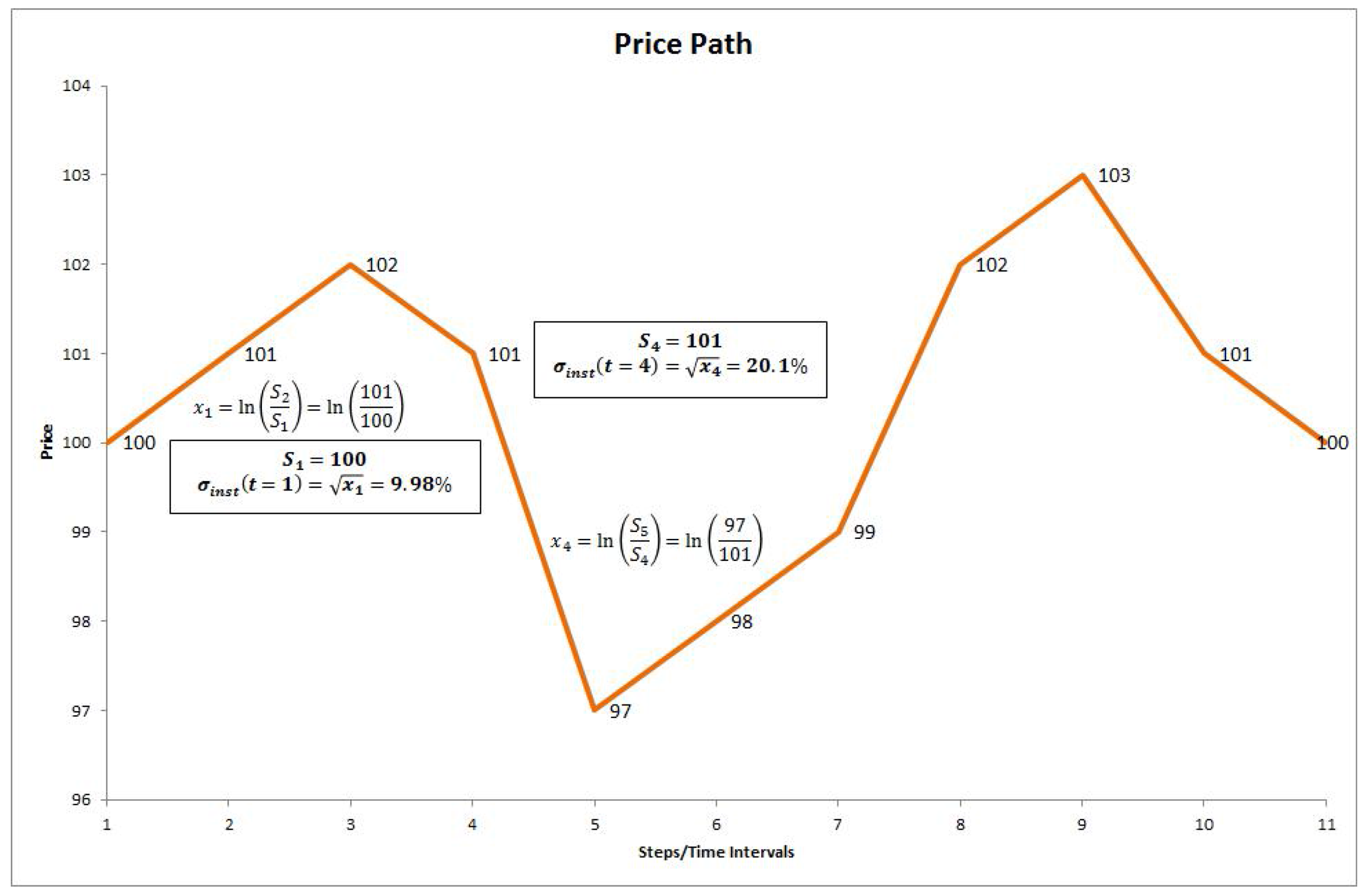
In its most general form, the function $\sigma (S,t)$ is called the instantaneous volatility for an option with time to expiry T and its dynamics are stochastic. Furthermore, similar to the definition of the instantaneous forward interest rate [36], we define the square of the at-the-money implied volatility as follows

$${\sigma }^2\left(T\right)=\frac{1}{T}{\int }_0^T{\sigma }^2\left(t\right)dt$$

(3.13)

by additivity of variance [27]. This shows that the implied volatility is a fair average, across time, over all instantaneous variances.

Readers might be confused due to the last paragraph in Section 2.1 and Equation (2.4) where we stated that the implied volatility is not a volatility after all. The instantaneous variance in Equation (3.13) is not the true variance of the stochastic process $S_t$. It is something different as explained by Rebonato [29] and in §2.1.

We further know that the Black-Scholes backward parabolic equation in variables S and t, given in Equation (2.6), is the Feynman-Kac representation of the discounted expected value of the final option value as given in Equation (2.7) [42].

Dupire [34] attempted to answer the question of whether it was possible to construct a state-dependent instantaneous volatility that, when fed into the one-dimensional diffusion equation given in Equation (3.12), will recover the entire implied volatility surface $\sigma (K,T)$? This suggests he wanted to know whether a deterministic volatility function exists that satisfies Equation (3.12). The answer to this question is negative, however, it becomes true if we apply Gyöngy’s theorem where the stochastic differential Equation in (3.12) is transformed to another SDE with a non-random volatility function. This is ultimately what Dupire proved.

According to standard financial theory, the price at time t of a call option with strike price K, maturity time T is the discounted expectation of its payoff, under the risk-neutral measure. Dupire assumed that the probability density of the underlying asset $S_t$ at the time t has to satisfy the forward Fokker-Planck Equation (also known as the forward Kolmogorov equation) given by [9]

$$\frac{\partial }{\partial t}\phi =\frac{1}{2}\frac{{\partial }^2}{\partial S_T^2}\left({\sigma }^2(S_T,T)S_T^2\phi \right)-S_t\frac{\partial }{\partial S_T}\left((r-d)S_T\phi \right)$$

(3.14)

where $\phi \equiv \phi (S_T,T)$ is the forward transition probability density of the random variable $S_T$ (final S at expiry time T) in the SDE shown in Equation (3.12) [27]. However, using the Breeden-Litzenberger formula [43]

$$\frac{{\partial }^{2}C}{\partial K^2}=\phi (K,T),$$

(3.15)

and doing a bit of calculus (see [27,33]), we can rewrite this and obtain the Dupire forward equation in terms of call option prices $C(K,T)$

$$\left[\frac{\partial }{\partial T}+(r-d)K\frac{\partial }{\partial K}-\frac{1}{2}{\sigma }^2(K,T)K^2\frac{{\partial }^2}{\partial K^2}+d\right]C(K,T)=0$$

(3.16)

where $\sigma (K,T)$ is continuous, twice-differentiable in strike and once in time, and local volatility is uniquely determined by the surface of call option prices. Note how, when moving from the backward Kolmogorov Equation (the Black-Scholes PDE given in Equation (2.3)) to the forward Fokker-Planck equation, the time to maturity T has replaced the calendar time t and the strike K has replaced the stock level S. The Fokker-Planck equation describes how a price propagates forward in time. This equation is usually used when one knows the distribution density at an earlier time, and one wants to discover how this density spreads out as time progresses, given the drift and volatility of the process [29]. Dupire’s forward equation also provides useful insights into the inverse problem of calibrating diffusion models to observed call and put option prices.

This forward PDE is very useful because it holds in a more general context than the backward PDE: even if the (risk-neutral) dynamics of the underlying asset is not necessarily Markovian, but described by a continuous Brownian martingale

$$d{S}_t=S_t\sigma d{W}_t$$

then call options still satisfy a forward PDE where the diffusion coefficient is given by the local (or effective) volatility function $\sigma (S,t)$ given by

$$\sigma (S,t)=\sqrt{\mathbb{E}\left[{\sigma }^2\right|S_t=S]}$$

and σ is the instantaneous or stochastic volatility of the process $S_t$. This method is linked to the Markovian projection problem: the construction of a Markov process which mimics the marginal distributions of a martingale. Such mimicking processes provide a method to extend the Dupire equation to non-Markovian settings (see Appendix A).

Dupire [9] used the strike/dual Gamma $({\partial }^{2}C/\partial K^2$) of a call option, that gives the marginal probability distribution function [43], and thought of this as timeslices of the forward transition probabilities. Now, since the forward Fokker-Planck equation in Equation (3.14) describes the time evolution of forward transition probabilities, we can isolate the volatility coefficients that recover the prices of tradable call options for all strikes and all times in Equation (3.16).

Dupire actually proved that it is possible to find the same option price solving a dual problem, namely a forward parabolic equation in the variables K and T known as the dual Black-Scholes equation or Dupire’s equation. This equation is actually the Fokker-Planck equation for the probability density function of the underlying asset integrated twice. This solution allows us to calculate the price of an European call option for every strike and maturity, given the present spot value S and time t.

Dupire solved for the volatility and got [9]

$${\sigma }_{loc}^2(K,\tau )=2\left\{\frac{{\displaystyle \frac{\partial C(K,\tau )}{{\displaystyle \partial \tau }}+C(K,\tau )d+(r-d)K\frac{\partial C(K,\tau )}{\partial K}}}{K^2\frac{{\displaystyle {\partial }^{2}C(K,\tau )}}{{\displaystyle \partial K^2}}}\right\}$$

(3.17)

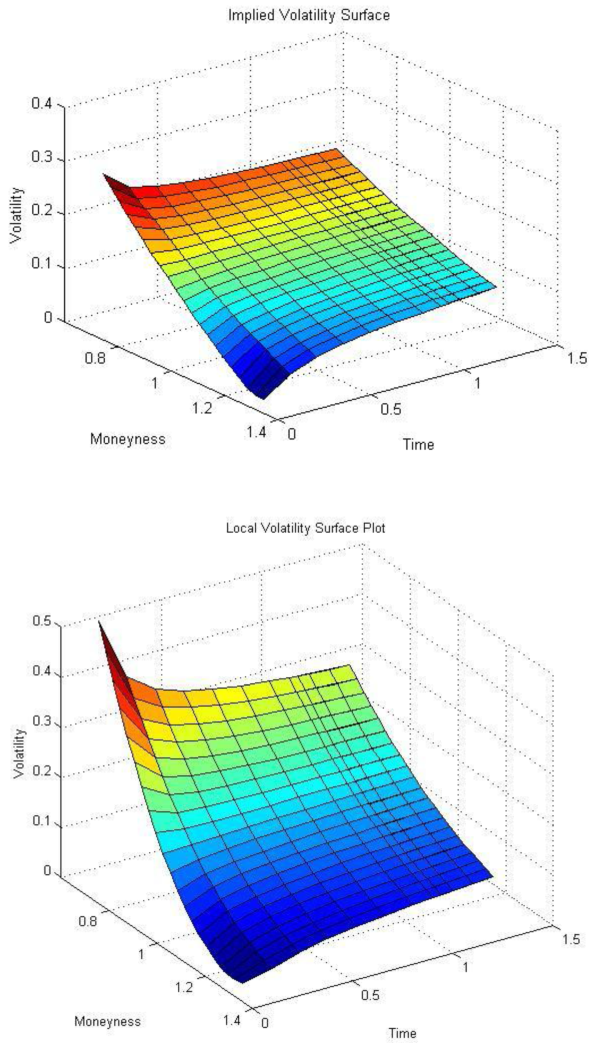
Thus, given prices for all plain-vanilla call options $C(K,\tau )$ today, ${\sigma }_{loc}(K,\tau )$ is the local volatility that will prevail at time τ when the future stock price is equal to K $(S_{\tau }=K)$. Note that we introduced a new time variable $\tau =T^{\prime }-t$ and $T^{\prime }$ where $t\le =T^{\prime }\le T$—call this an interim expiry date. The reason is that it facilitates the calculation and plotting of the whole surface from t to the expiry date T. We now have that t and $S_0$ are respectively the market date, on which the volatility smile is observed, and the asset price on that date. To calculate the local volatility at each time point from t to the expiry time T, we let $T^{\prime }$ move forward in time while we keep t constant. To plot the 3D surface, start at the valuation date t, move forward in time by a small amount to a new $T^{\prime }$; for example a day or a week. Calculate τ and vary the strikes to calculate ${\sigma }_{loc}(K,\tau )$. Move forward to a new $T^{\prime }$ and do the same until one ends at $T^{\prime }=T$.

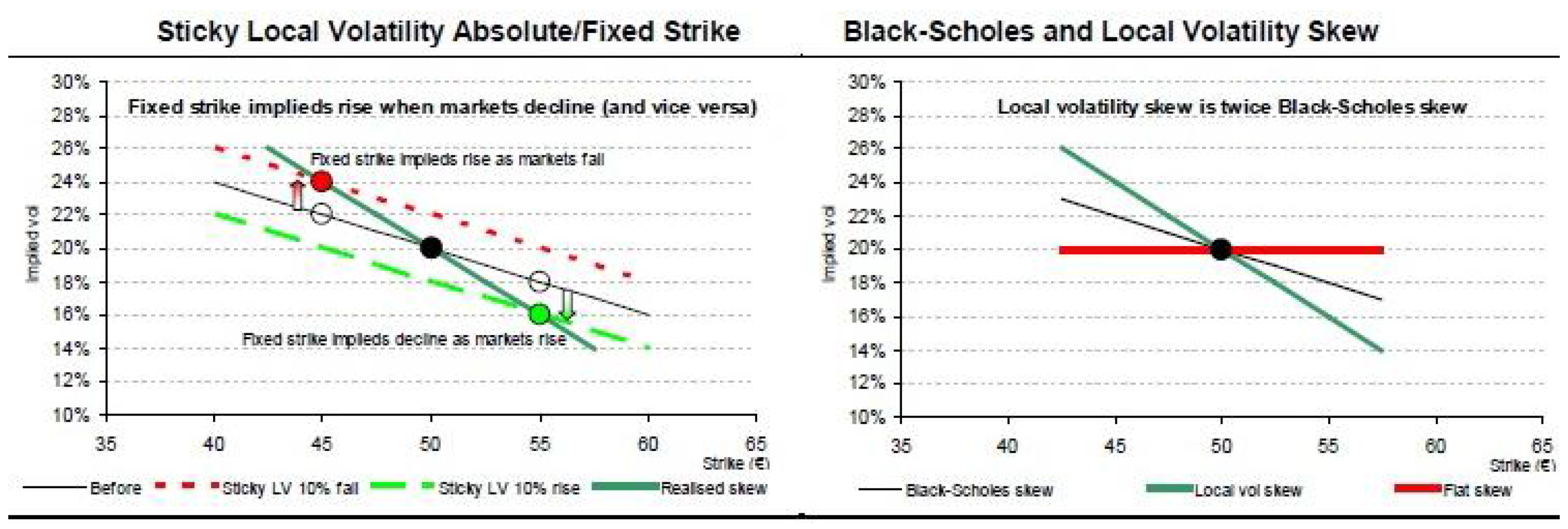
Note that r is a fixed interest rate and d a fixed dividend yield, both in continuous format. See the number 2 on the right hand side of Equation (3.17). This backs our statement in Section 3.3.3 up where we stated that the implied volatility is half the local volatility skew. Note that Equation (3.17) ensures the existence and uniqueness of a local volatility surface which reproduces the market prices exactly.

We further note that for Equation (3.17) to make sense, the right hand side must be positive. How can we be sure that volatilities are not imaginary? This is guaranteed by no-arbitrage arguments. We have from the denominator

$${\sigma }_{loc}^2(K,T)\propto {\left(K^2\times \frac{{\partial }^{2}C}{\partial K^2}\right)}^{-1}$$

$K^2$ is positive always and, the dual gamma or risk-neutral price density must be positive in the absence of arbitrage (butterfly spread). To ensure the positivity of the numerator, we note that no-arbitrage arguments state that calendar spreads should have positive values. Kotzé and Joseph [44] and Kotzé et al. [18] discusses no-arbitrage arguments in detail. We can turn these statements around: An implied volatility surface is arbitrage free if the local volatility is a positive real number (not imaginary) where ${\sigma }_{loc}(K,T)\in {\mathbb{R}}_0^{+}$.

Dupire’s Equation (3.17) is not analytically solvable. The option price function (and the derivatives) in this equation have to be approximated numerically. The derivatives are easily obtained in using Newton’s difference quotient. To obtain the dual delta, $\partial C/\partial K$, we therefore use

$$\frac{\partial C(K,T)}{\partial K}=\frac{C(K+\Delta K,\sigma (K+\Delta K,T\left)\right)-C(K,\sigma (K,T\left)\right)}{\Delta K}$$

(3.18)

where we note that all calls should be priced with the implied volatility smile. Here, $C(K+\Delta K,\sigma (K+\Delta K,T\left)\right)$ denotes a call price at a strike of $K+\Delta K$ where the implied volatility is found from the implied volatility skew for this option expiring at T with a strike of $K+\Delta K$. To find an optimal size of the bump, $\Delta K$, it should be tested for. For an index like the Top 40, one or ten index points works very well but some people prefer it to be a percentage of the strike price. Be careful not to make it too big—1% might seem small but it is in general too big. One or ten basis points works rather well for the change in time interval.

Further note that one cannot use the closed-form Black-Scholes derivatives for the dual delta. We call the numeric dual delta in Equation (3.18), the impact/modified dual delta. Traders call the ordinary delta calculated this way, i.e., with the skew, the impact/modified delta due to the fact that it gives a truer reflection (or impact) of the dynamic hedging process—it takes some of the nonlinear effects of the Black-Scholes equation, together with the shape of the volatility skew, into account. The dual gamma is numerically obtained by

$$\frac{{\partial }^{2}C(K,T)}{\partial K^2}=\frac{C(K+\Delta K,\sigma (K+\Delta K\left)\right)+C(K-\Delta K,\sigma (K-\Delta K\left)\right)-2C(K,\sigma (K\left)\right)}{\Delta K^2}$$

where we dropped the T for clarity’s sake [29].

Unfortunately there are practical issues with Equation (3.17). Problems can arise when the values to be approximated are very small and small absolute errors in the approximation can lead to big relative errors, perturbing the estimated quantity heavily. Determining the density ${\partial }^{2}C/\partial K^2$ is numerically delicate. It is very small for options that are far in- or out-of-the-money (the effect is particularly large for options with short maturities). Small errors in the approximation of this derivative will get multiplied by the strike value squared resulting in big errors at these values, sometimes even giving negative values, resulting in negative variances and complex local volatilities. The local volatility will remain finite and well-behaved only if the numerator approaches zero at the right speed for these cases.

Further to the numerical issues, the continuity assumption of option prices is, of course, not very realistic. In practice option prices are known for certain discrete points and at limited number of maturities (quarterly for instance like most Safex options). The result of this is that in practice the inversion problem is ill-posed i.e., the solution is not unique and is unstable—the positivity of the second derivative in the strike direction is not guaranteed.

3.6. Local Volatility in terms of Implied Volatility

The instability of Equation (3.17) forces us to consider alternatives. We know options are traded in the market on implied volatility and not price. Can we thus not transform this equation such that we supply the implied volatilities instead of option prices?

This can be done if a change of variables is made in Equation (3.17) by rewriting the Black-Scholes equation for a call C in terms of the log-strike y where $y=log(strike/forward)$. This leads to [23,27]

$${\displaystyle {\sigma }_{loc}^2(K,\tau )=\frac{{\displaystyle {\sigma }_{imp}^2+2\tau {\sigma }_{imp}\frac{{\displaystyle \partial {\sigma }_{imp}}}{{\displaystyle \partial \tau }}+2(r-d)K\tau {\sigma }_{imp}\frac{{\displaystyle \partial {\sigma }_{imp}}}{\partial K}}}{{\left(1+K{d}_1\sqrt{\tau }\frac{{\displaystyle \partial {\sigma }_{imp}}}{{\displaystyle \partial K}}\right)}^2+K^2\tau {\sigma }_{imp}\left(\frac{{\displaystyle {\partial }^2{\sigma }_{imp}}}{{\displaystyle \partial K^2}}-d_1\sqrt{\tau }{\left({\displaystyle \frac{{\displaystyle \partial {\sigma }_{imp}}}{{\displaystyle \partial K}}}\right)}^2\right)}}$$

(3.19)

where

$$d_1=\frac{ln\left({\displaystyle S_0/K}\right)+\left((r-d)+{\sigma }_{imp}^2/2\right)\tau }{{\sigma }_{imp}\sqrt{\tau }}$$

and ${\sigma }_{imp}\equiv {\sigma }_{imp}(K,\tau )$ where $\tau =T-t$ such that t and $S_0$ are respectively the market date, on which the volatility smile is observed, and the asset price on that date. Note that Equation (3.19) gives the variance, i.e., ${\sigma }^2$. See the explanation following Equation (3.17) on how the new variable τ facilitates the plotting of the whole local volatility surface.

When comparing Equations (3.17) and (3.19) it is clear that the problem of numerical large errors no longer exists. The transformation of Dupire’s formula into one which depends on the implied volatility ensures that the dual Gamma is no longer alone in the denominator as it was in Equation (3.17). The second derivative of the implied volatility is now one term of a sum, so small errors in it will not necessarily lead to large errors in the local volatility function. However, small differences in the input volatility surface can produce a big difference in the estimated local volatility.

The main problem is that the implied or traded volatilities are only known at discrete strikes K and expiries T. This is why the parameterisation chosen for the implied volatility surface is very important. If implied volatilities are used directly from the market, the derivatives in Equation (3.19) need to be obtained numerically using finite difference or other well-known techniques. This can still lead to an unstable local volatility surface. Furthermore we will have to interpolate and extrapolate the given data points unto a surface. Since obtaining the local volatility from the data involves taking derivatives, the extrapolated implied volatility surface cannot be too uneven. If it is, this unevenness will be exacerbated in the local volatility surface showing that it is not arbitrage free in these areas.

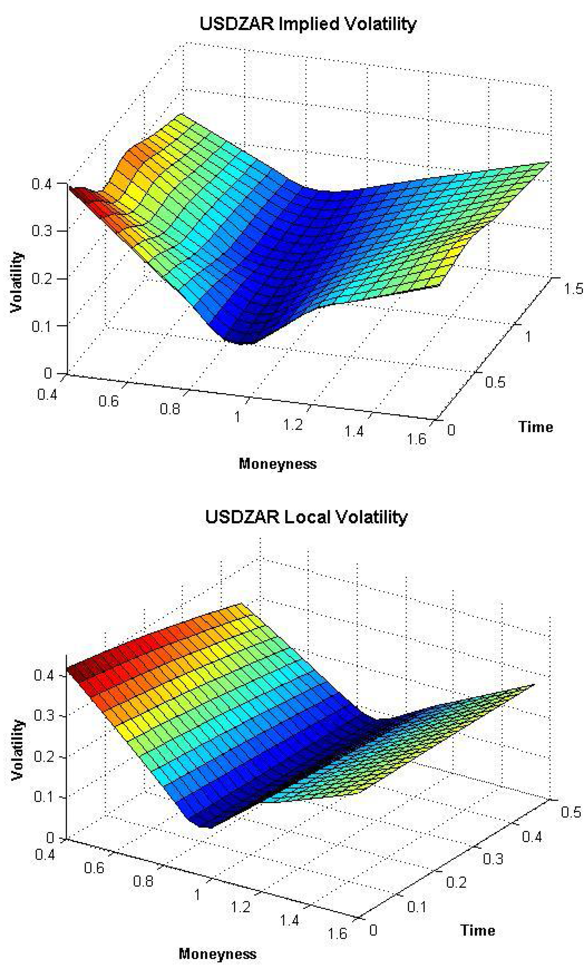
In the foreign exchange market, options are traded on the Delta—effectively a measure of the moneyness—as opposed to the absolute level of the strike. See Clark [27] for the FX version of Equation (3.19).

4. The ALSI: Exact Implementation of the DVF

4.1. The Deterministic Implied Volatility Function

The issues relating to determining the derivatives in Equation (3.19) are circumvented in two ways. One can either choose a particular functional form for the implied volatility surface and fit this function to the market volatility data, or one can choose a particular functional form for the local volatility surface and find it using non-linear optimization techniques.

Safex chose the first way for the liquid ALSI options and uses the following Three-parameter deterministic quadratic function as a good model of fit for the ALSI implied volatility data on every expiry date (for a full discussion see [18,44])

$${\sigma }_{\mathrm{model}}({\beta }_0,{\beta }_1,{\beta }_2,T_k)={\beta }_0^k+{\beta }_1^{k}M+{\beta }_2^k{M}^2$$

(4.20)

$T_k$ are the times to expiry for all listed expiry dates such that $k=1,2,\dots ,n$ and n is the total number of listed expiries. Note that the ALSI options traded on Safex are options on a futures contract—the ALSI is the liquid futures contract on the FTSE/JSE Top 40 tradable index. In all of the analysis below we assume that the spot price of the ALSI is the futures level F.

This equation, of course, describes a parabola (for each expiry) and this conic section has the following properties (dropping the superscript k)

• $M=K/F$ is the strike price in moneyness format (Strike/Future),
• ${\beta }_0$ is the constant volatility (shift or trend or level) parameter, ${\beta }_0>0$. Note that

  $$\underset{M\to 0}{\sigma \to {\beta }_0}$$

  This means that ${\beta }_0$ is similar to the Y-intercept for a parabola. We have, in the Cartesian plane, the Y-axis being ${\sigma }_{\mathrm{model}}$ and the X-axis being the moneyness.
• ${\beta }_1$ is the correlation (slope) term. This parameter accounts for the negative correlation between the underlying index and volatility. The no-spread-arbitrage condition requires that $-1<{\beta }_1<0$.
• ${\beta }_2$ is the volatility of volatility (“vol of vol” or curvature/convexity) parameter. The no-calendar-spread arbitrage convexity condition requires that ${\beta }_2>0$.

Note that Equation (4.20) is linear in the wings8 if $M\to \pm \infty$ and it holds for discrete expiry time T. The linearity of the skew in the wings is a well-known empirical fact and it was proven mathematically by Lee [46] and extended by Benaim and Friz [45]. Lee proved that the implied variance is linear in strike for very small en very large strikes. These properties and constraints are the factors describing the shape of the skews—they are not the no-arbitrage constraints. They are, however, related to the no-arbitrage conditions imposed on a volatility skew and surface—these are discussed in [18].

The n parabolas described by Equation (4.20) can now be fitted to the relevant option data (obtained per expiry date) independently to give us n discrete skews. In order to incorporate the time dependence and generate a continuous smooth implied volatility surface we also need a specification or functional form for the at-the-money (ATM) volatility term structure. It is, however, important to remember that the ATM volatility is intricately part of the skew. This infers that the two optimizations (one for the skews and the other for the ATM volatilities) cannot be done strictly separate from one another. Taking the ATM term structure together with each skew will give us the 3D implied volatility surface.

It is well-known that volatility is mean reverting; when volatility is high (low) the volatility term structure is downward (upward) sloping [33]. Safex uses the following exponential functional form for the ATM volatility term structure

$${\sigma }_{\mathrm{atm}}(M,t)=\frac{\theta }{t^{\lambda }}$$

(4.21)

Here we have (See [44] for full details)

• t is the time to expiry,
• λ controls the overall slope of the ATM term structure; $\lambda >0$ implies a downward sloping ATM volatility term structure, whilst a $\lambda <0$ implies an upward sloping ATM volatility term structure, and
• θ controls the short term ATM curvature.

We now assume that each of the parameters β in Equation (4.20) must satisfy Equation (4.21) such that

$${\beta }_i\left(t\right)=\frac{{\theta }_i}{t^{{\lambda }_i}};i=0,1,2$$

(4.22)

To ensure the surface is continuous we dropped the superscript k and changed the discrete expiry times $T_k$ to a continuous time t where $T_k\in t;t\in {\mathbb{R}}_0^{+}$. Combining Equations (4.20) and (4.22) leads to

$${\sigma }_{imp}(M,t)=\frac{{\theta }_0}{t^{{\lambda }_0}}+\frac{{\theta }_1}{t^{{\lambda }_1}}M+\frac{{\theta }_2}{t^{{\lambda }_2}}{M}^2$$

(4.23)

Equation (4.23) fully describes the 3D implied volatility surface. We have to find 6 parameters by fitting this function to the market volatility skews using optimization techniques. From Equation (4.21) we know that λ controls the slope of the curves (we also call this the scaling parameters) while θ controls the curvature. From Equation (4.20) we thus have

• ${\beta }_0$ and ${\lambda }_0$ are called the level or shift or trend parameters and they control the level of the volatility.
• ${\beta }_1$ and ${\lambda }_1$ are called the rho or tilt parameters and they control the overall slope of the curves.
• ${\beta }_2$ and ${\lambda }_2$ are the volatility of volatility parameters and they control the curvature.

Kotzé and Joseph [44] mention they use a floating surface such that $M_{\mathrm{ATM}}=1$ i.e., the ATM strike is one. A floating surface is defined such that

$${\sigma }_{\mathrm{imp}}(M,t)={\sigma }_{\mathrm{ATM}}\left(t\right)+{\sigma }_{\mathrm{imp}}^{float}(M,t)$$

(4.24)

where ${\sigma }_{\mathrm{ATM}}\left(t\right)$ is the market at-the-money volatility.

Now, from Equation (4.23) we have

$${\sigma }_{imp}^{\mathrm{ATM}}\left(t\right)=\frac{{\theta }_0}{t^{{\lambda }_0}}+\frac{{\theta }_1}{t^{{\lambda }_1}}+\frac{{\theta }_2}{t^{{\lambda }_2}}$$

(4.25)

Thus, combining Equations (4.23)–(4.25) leads us to the final 3 dimensional market volatility surface given by (transforming back from moneyness to the real world i.e., substituting $M=K/F$)

$${\sigma }_{\mathrm{imp}}(F,K,t)={\sigma }_{\mathrm{ATM}}\left(t\right)+\frac{{\theta }_1}{t^{{\lambda }_1}}\left(\frac{K}{F}-1\right)+\frac{{\theta }_2}{t^{{\lambda }_2}}\left({\left(\frac{K}{F}\right)}^2-1\right)$$

(4.26)

Safex obtains the ATM volatilities from the market meaning ${\sigma }_{\mathrm{ATM}}\left(t\right)$ is a constant for every t.

Safex publishes two other parameters: ${\theta }_A$ and ${\lambda }_A$. These parameters are the at-the-money parameters from Equation (4.21) and gives the theoretical ATM term structure of volatility. They are obtained by fitting Equation (4.21) to the market (or mark-to-market (MtM)) term structure of ATM volatilities ${\sigma }_{\mathrm{MtM}}^{\mathrm{ATM}}\left(t\right)$ such that

$${\sigma }_{\mathrm{model}}^{\mathrm{ATM}}\left(t\right)=\frac{{\theta }_A}{t^{{\lambda }_A}}\simeq {\sigma }_{\mathrm{MtM}}^{\mathrm{ATM}}\left(t\right)$$

(4.27)

Using them in calculating the ATM volatilities will give slightly different values if compared to the at-the-money volatilities calculated using Equation (4.25). The reason is that ${\theta }_A$ and ${\lambda }_A$ are obtained by fitting Equation (4.21) to the raw ATM volatility data while the other θ’s and λ’s are obtained by optimizing the whole surface and by taking the no-arbitrage conditions into account (see [44]).

We need to mention a practical implementation point here. The term structure of ATM volatilities as obtained from the model in Equation (4.27) will not coincide with all the traded or mark-to-market ATM volatilities due to the numerical fitting procedure. We must, however, ensure that if we price an option expiring on a particular date, that ${\sigma }_{\mathrm{ATM}}\left(t\right)$ in Equation (4.26) equates the market ATM volatility for that date. As an example, if we price a 9 month option ($T=0.75$) and we have the 9 month mark-to-market ATM volatility ${\sigma }_{\mathrm{MtM}}^{\mathrm{ATM}}(0.75)$, we need to ensure that ${\sigma }_{\mathrm{ATM}}(0.75))$ in Equation (4.26) is equal to this volatility. This is achieved by floating ${\sigma }_{\mathrm{model}}^{\mathrm{ATM}}\left(t\right)$ up or down by a constant amount such that ${\sigma }_{\mathrm{ATM}}(0.75)={\sigma }_{\mathrm{MtM}}^{\mathrm{ATM}}(0.75)={\sigma }_{\mathrm{model}}^{\mathrm{ATM}}(0.75)$. This will in general have the effect that ${\sigma }_{\mathrm{ATM}}\left(t\right)$ is not equal to the mark-to-market volatilities for $t\ne 0.75$.

The whole volatility surface is now described by a functional form given in Equation (4.26). The derivatives in Dupire’s local volatility function in Equation (3.19) can now be obtained analytically such that we have from Equation (4.26)

$$\begin{array}{ccc}\hfill \frac{\partial {\sigma }_{imp}(F,K,t)}{\partial K}& =& \frac{1}{F}\frac{{\theta }_1}{t^{{\lambda }_1}}+2\frac{K}{F^2}\frac{{\theta }_2}{t^{{\lambda }_2}}\hfill \\ \hfill \frac{{\partial }^2{\sigma }_{imp}(F,K,t)}{\partial K^2}& =& 2\frac{1}{F^2}\frac{{\theta }_2}{t^{{\lambda }_2}}\hfill \\ \hfill \frac{\partial {\sigma }_{imp}(F,K,t)}{\partial t}& =& -{\lambda }_1{\theta }_1{t}^{-({\lambda }_1+1)}\left(\frac{K}{F}-1\right)-{\lambda }_2{\theta }_2{t}^{-({\lambda }_2+1)}\left({\left(\frac{K}{F}\right)}^2-1\right)\hfill \end{array}$$

(4.28)

Using Equations (4.28) will lead to a smooth Dupire local volatility function for ${\sigma }_{loc}(K,T))$ in Equation (3.19). Further, if the implied volatility surface in Equation (4.26) is arbitrage-free, the corresponding Dupire local volatility surface should be arbitrage-free as well.

Equations (4.26) and (4.28) can now be substituted into Dupire’s equation in Equation (3.19) such that we calculate the local volatility surface algebraically across time and strike.

4.2. The ALSI Implied and Local Volatilities

It is now pretty straight forward to obtain the local volatility surface for ALSI options. We need the four parameters, ${\theta }_1,{\theta }_2,{\lambda }_1$ and ${\lambda }_2$ and the published ATM volatilities. These parameters are published every two weeks when Safex updates its volatility surfaces.

In Table 2 we show the parameter values, ${\theta }_i$ and ${\lambda }_i$, $(i=1,2,3,ATM)$ as published by Safex on 28 May 2014. Also shown are the values for ${\theta }_i/t^{{\lambda }_i},i=0,1,2,3$. Table 3 lists ${\sigma }_{\mathrm{imp}}^{\mathrm{ATM}}$, the model ATM volatilities and official Safex ATM volatilities for all expiry dates. In Figure 6 we show the ALSI implied and corresponding local volatility surfaces.

Table 2. Optimized parameters for the ALSI deterministic implied volatility function on 28 May 2014 (see Equations (4.24)–(4.26)).

		Curvature
		Rho(${\theta }_1$)	VolVol (${\theta }_2$)	Level (${\theta }_0$)	Atm (${\theta }_{\mathrm{ATM}}$)
	In Months	–0.8488985	0.1945430	0.9139862	0.1350075
	In Years	–0.4337514	0.1069264	0.4753064	0.1595808
		Decay
		Rho (${\lambda }_1$)	VolVol (${\lambda }_2$)	Level (${\lambda }_0$)	Atm (${\lambda }_{\mathrm{ATM}}$)
		0.2702186	0.2408592	0.2631310	–0.0672942
Date	T	${\theta }_1/t^{{\lambda }_1}$	${\theta }_2/t^{{\lambda }_2}$	${\theta }_0/t^{{\lambda }_1}$
19 June 2014	0.06027397	–92.655786%	21.033029%	99.531201%
18 September 2014	0.30958904	–59.544292%	14.181881%	64.708854%
18 December 2014	0.55890411	–50.759237%	12.301016%	55.393271%
19 March 2015	0.80821918	–45.943944%	11.255306%	50.269616%
18 June 2015	1.05753425	–42.724414%	10.549535%	46.836131%
17 September 2015	1.30684932	–40.349172%	10.025150%	44.298712%
15 December 2016	2.55342466	–33.668883%	8.531503%	37.140432%
21 December 2017	3.56986301	–30.754183%	7.869980%	34.005870%

Table 2. Optimized parameters for the ALSI deterministic implied volatility function on 28 May 2014 (see Equations (4.24)–(4.26)).

		Curvature
		Rho(${\theta }_1$)	VolVol (${\theta }_2$)	Level (${\theta }_0$)	Atm (${\theta }_{\mathrm{ATM}}$)
	In Months	–0.8488985	0.1945430	0.9139862	0.1350075
	In Years	–0.4337514	0.1069264	0.4753064	0.1595808
		Decay
		Rho (${\lambda }_1$)	VolVol (${\lambda }_2$)	Level (${\lambda }_0$)	Atm (${\lambda }_{\mathrm{ATM}}$)
		0.2702186	0.2408592	0.2631310	–0.0672942
Date	T	${\theta }_1/t^{{\lambda }_1}$	${\theta }_2/t^{{\lambda }_2}$	${\theta }_0/t^{{\lambda }_1}$
19 June 2014	0.06027397	–92.655786%	21.033029%	99.531201%
18 September 2014	0.30958904	–59.544292%	14.181881%	64.708854%
18 December 2014	0.55890411	–50.759237%	12.301016%	55.393271%
19 March 2015	0.80821918	–45.943944%	11.255306%	50.269616%
18 June 2015	1.05753425	–42.724414%	10.549535%	46.836131%
17 September 2015	1.30684932	–40.349172%	10.025150%	44.298712%
15 December 2016	2.55342466	–33.668883%	8.531503%	37.140432%
21 December 2017	3.56986301	–30.754183%	7.869980%	34.005870%

Table 3. Model and official Safex at-the-money (ATM) volatilities on 28 May 2014.

Expiry Date	Expiry Time T	Model ATM ${\sigma }_{\mathrm{model}}^{\mathrm{ATM}}\left(t\right)$	Safex ATM ${\sigma }_{\mathrm{MtM}}^{\mathrm{ATM}}\left(t\right)$
19 June 2014	0.06027397	13.209622%	14.25
18 September 2014	0.30958904	14.747329%	14.00
18 December 2014	0.55890411	15.345386%	14.50
19 March 2015	0.80821918	15.731053%	15.00
18 June 2015	1.05753425	16.018262%	15.75
17 September 2015	1.30684932	16.248072%	16.75
15 December 2016	2.55342466	16.997206%	18.50
21 December 2017	3.56986301	17.384842%	21.00

Table 3. Model and official Safex at-the-money (ATM) volatilities on 28 May 2014.

Expiry Date	Expiry Time T	Model ATM ${\sigma }_{\mathrm{model}}^{\mathrm{ATM}}\left(t\right)$	Safex ATM ${\sigma }_{\mathrm{MtM}}^{\mathrm{ATM}}\left(t\right)$
19 June 2014	0.06027397	13.209622%	14.25
18 September 2014	0.30958904	14.747329%	14.00
18 December 2014	0.55890411	15.345386%	14.50
19 March 2015	0.80821918	15.731053%	15.00
18 June 2015	1.05753425	16.018262%	15.75
17 September 2015	1.30684932	16.248072%	16.75
15 December 2016	2.55342466	16.997206%	18.50
21 December 2017	3.56986301	17.384842%	21.00

Continuing with our example in the previous section: if we want to price an 18 Dec 2014 ALSI option, we will have to float the model ATMs down by 0.15345386-0.145=0.00845386.

From Figure 6 we notice that the implied volatility surface does not have a lot of curvature—it is skewed but flat. However, we also see from the local volatility surface that it has more curvature. This shows that the local volatility skew is twice that of the implied volatility as stated in Section 3.3.3.

Figure 6. ALSI implied and local volatility surfaces on 28 May 2014.

Figure 6. ALSI implied and local volatility surfaces on 28 May 2014.

5. Numerical Implementation of Dupire

In Section 4.1 we described the methodology implemented for obtaining the ALSI volatility surface and how the Dupire local volatility surface can be calculated algebraically. Unfortunately, such deterministic functions for the implied volatility surfaces for some of the other instruments like the DTOP and USDZAR (US Dollar and South African Rand exchange rate), do not exist. The implied volatility surfaces are, however, available, albeit in a discrete form. All derivatives in Equation (3.19) have to be computed numerically. The procedures and methodologies implemented at the JSE are discussed in this section.

5.1. Volatility Interpolation and Extrapolation

In practice, we are often confronted with situations where only limited amounts of data are accessible and it is necessary to estimate values between two consecutive given data points. We can construct new points between known data points by interpolation or smoothing techniques.

All implied volatility surfaces used by the JSE are available online9. The volatility surface (first 4 expiries) for the DTOP10 as published on 28 May 2014 is shown in Figure 7. Only a handful of discrete points are given.

Figure 7. DTOP Please define if necessary volatility surface as published by the Johannesburg Stock Exchange (JSE) on 28 May 2014.

Figure 7. DTOP Please define if necessary volatility surface as published by the Johannesburg Stock Exchange (JSE) on 28 May 2014.

Inter- and extrapolation is thus necessary. At the JSE, we take the volatilities, square them and do linear inter- and extrapolation on the variance. However, it is a two-dimensional problem. We have to do this across strike and across time. If you just need to interpolate across strike prices use the following

$${\sigma }^2\left(K\right)={\sigma }_1^2+({\sigma }_2^2-{\sigma }_1^2)\frac{K-K_1}{K_2-K_1}$$

Here we want to find the variance for a certain strike given by K where $K_1\le K\le K_2$ and the volatility at $K_1$ is ${\sigma }_1$ and that at $K_2$ is ${\sigma }_2$. Further, ${\sigma }_1^2\le {\sigma }^2\le {\sigma }_2^2$.

When we interpolate across time only, we use what is known as flat forward interpolation. Volatility is time dependent. Suppose that N time points $t_0=0,t_1,t_2,\dots ,t_N$ are given, and the implied volatilities for each of these time points are ${\sigma }_1,{\sigma }_2,\dots ,{\sigma }_N$. We now define a general interpolation scheme to find the volatility at any time point t where $t\in {\mathbb{R}}_0^{+}$ such that [27]

$$\sigma \left(t\right)=\left\{\begin{array}{cc}{\sigma }_1,\hfill & \hfill t<t_1\\ {\displaystyle \sqrt{\frac{1}{t}\left[{\sigma }_i^2{t}_i+{\sigma }_{i,i+1}^2(t-t_i)\right]},}\hfill & \hfill t_i\le t<t_{i+1}fori<N\\ {\sigma }_N,\hfill & \hfill t\ge t_N\end{array}\right.$$

(5.29)

where

$${\sigma }_{i,i+1}^2=\frac{{\sigma }_{i+1}^2{t}_{i+1}-{\sigma }_i^2{t}_i}{t_{i+1}-t_i}$$

5.2. Safex’s Implementation

We use the following 3 steps when we want to implement Dupire’s equation in Equation (3.19) for all instruments except the ALSI

• Read in the implied volatility surface as published by the JSE and convert it to a floating and moneyness format;
• Regularize the surface, meaning we interpolate and plot it with more than the given 9 strikes per expiry;
• Use this regularized implied volatility surface when we transform it to the local volatility surface.

The first step encompasses the format of how the skew is read into our model. All volatility surfaces are given in the format as shown in Figure 7. This is converted to a floating surface where the strikes are given in terms of moneyness. Moneyness is ($K/S$) and is just the percentage of how far the strike is in- or out-the-money. This is shown in Table 4.

Table 4. Floating DTOP skews for 3 expiry times on 28 May 2014.

DTOM4	19 June 2014	DTOU4	18 September 2014	DTOZ4	18 December 2014
70.2600%	16.4700%	69.9000%	10.4200%	70.2000%	8.6500%
80.0000%	10.6700%	80.1000%	6.6000%	80.3000%	5.4700%
90.2600%	4.9900%	90.3100%	3.0800%	89.9000%	2.6900%
95.3800%	2.3100%	95.4100%	1.4200%	94.9500%	1.3100%
100.0000%	0.0000%	100.0000%	0.0000%	100.0000%	0.0000%
105.1300%	–2.4700%	105.1000%	–1.5100%	105.0500%	–1.2500%
110.2600%	–4.8300%	110.2000%	–2.9500%	110.1000%	–2.4400%
120.0000%	–9.0000%	120.4100%	–5.6000%	120.2000%	–4.6200%
130.2600%	–12.9700%	130.1000%	–7.8500%	130.3000%	–6.5600%

Table 4. Floating DTOP skews for 3 expiry times on 28 May 2014.

DTOM4	19 June 2014	DTOU4	18 September 2014	DTOZ4	18 December 2014
70.2600%	16.4700%	69.9000%	10.4200%	70.2000%	8.6500%
80.0000%	10.6700%	80.1000%	6.6000%	80.3000%	5.4700%
90.2600%	4.9900%	90.3100%	3.0800%	89.9000%	2.6900%
95.3800%	2.3100%	95.4100%	1.4200%	94.9500%	1.3100%
100.0000%	0.0000%	100.0000%	0.0000%	100.0000%	0.0000%
105.1300%	–2.4700%	105.1000%	–1.5100%	105.0500%	–1.2500%
110.2600%	–4.8300%	110.2000%	–2.9500%	110.1000%	–2.4400%
120.0000%	–9.0000%	120.4100%	–5.6000%	120.2000%	–4.6200%
130.2600%	–12.9700%	130.1000%	–7.8500%	130.3000%	–6.5600%

In Table 4 the first row contains the contract codes and skew dates. The first column gives the strikes in moneyness format. The second columns give the floating or relative volatilities. These are the volatilities relative to the at-the-money (ATM) volatilities. As an example, if the future level was 9898 (we call this the at-the-money level) for the 18 December 2014 expiry, we would describe the ATM volatility as the fair volatility to trade an option with a strike of 9898. We would then expect the 10,898 ($9898\times 110.1\%$) strike to trade at a volatility of –2.44% relative to the ATM volatility or 2.44% below the ATM volatility. If the ATM volatility was 14.5%, the fair value volatility for this option with a strike of 10,898 would be 12.06%.

Crucial: we need the ATM volatilities. These are published by Safex daily. We show the data for the DTOP as published on 28 May 2014 in Table 5. The second last column is empty because none of the ATM volatilities changed from the previous day.

Table 5. DTOP mark-to-market (MtM) data on 28 May 2014.

					VOL.	PREV.
DTOP	SPOT	BID	OFFER	M-T-M	CHANGES	VOLS.
19 June 2014	9727	9757	9757	9757		13.00
18 September 2014	9727	9807	9807	9807		14.00
18 December 2014	9727	9898	9898	9898		14.50
19 March 2015	9727	10015	10015	10015		14.50
18 June 2015	9727	10059	10059	10059		14.50
17 December 2015	9727	10249	10249	10249		14.50

Table 5. DTOP mark-to-market (MtM) data on 28 May 2014.

					VOL.	PREV.
DTOP	SPOT	BID	OFFER	M-T-M	CHANGES	VOLS.
19 June 2014	9727	9757	9757	9757		13.00
18 September 2014	9727	9807	9807	9807		14.00
18 December 2014	9727	9898	9898	9898		14.50
19 March 2015	9727	10015	10015	10015		14.50
18 June 2015	9727	10059	10059	10059		14.50
17 December 2015	9727	10249	10249	10249		14.50

The reason for using floating skews is the fact that the SAFEX systems, Nutron and Nuclears, use them in this way. Equity skews are updated every second week only. Between updates, the skews “float” up and down stuck to the ATM volatility at the 100% strike. The ATM volatilities are published, and these might change, on a daily basis. Changes are shown in the column “Changes” (second last) in Table 5. If this is empty, use the last column as the current ATM volatilities.

Important note:

• When we price an exotic option, we use the theoretical forward levels and not the published futures level. The reason being that barriers, for instance, are always on the cash level and not the futures level. We thus use

  $$F=S{e}^{(r-d)T}$$

  when calculating the forward. We thus need the following inputs.

  −

  Spot or cash level S: this is the current spot price of the underlying shown in column two in Table 5.

  −

  The current valuation date and expiry date. We then have

  $$T=\frac{\mathrm{Expiry\; Date}-\mathrm{Valuation\; Date}}{365}$$

  which is the annual time to expiry11.

  −

  ATM volatility for each expiry date. This is given in the last column of Table 5.

  −

  EndDate: The Date that the ATM volatility is applicable for. More specifically the expiry date of the option.

  −

  The current continuous compounding interest rate r. Obtained from the official JSE zero coupon swap yield curve.

  −

  The current continuous compounding dividend rate d. Obtained from Bloomberg.

Let us do an exercise on how to convert the floating skews back into absolute values—these are after all the values we are going to use. On 22 May 2014 we have the following for the DTOP (see Table 5): Spot/cash level = 9727, Forward level = 9898, Valuation date = 28 May 2014, ATM volatility = 14.50%, Expiry Date = 18 December 2014, r = 6.11% and d = 2.98%. Using these values lead us to the volatility skews shown in Table 6.

Table 6. DTOP implied volatility skews in absolute terms, using inputs as shown.

DTOM4	19 June 14	DTOU4	18 September 14	DTOZ4	18 December 14
6847	30.9700%	6865	24.9200%	6949	23.1500%
7796	25.1700%	7867	21.1000%	7948	19.9700%
8796	19.4900%	8870	17.5800%	8899	17.1900%
9295	16.8100%	9371	15.9200%	9399	15.8100%
9745	14.5000%	9822	14.5000%	9898	14.5000%
10245	12.0300%	10322	12.9900%	10398	13.2500%
10745	9.6700%	10823	11.5500%	10898	12.0600%
11694	5.5000%	11826	8.9000%	11898	9.8800%
12694	1.5300%	12778	6.6500%	12898	7.9400%

Table 6. DTOP implied volatility skews in absolute terms, using inputs as shown.

DTOM4	19 June 14	DTOU4	18 September 14	DTOZ4	18 December 14
6847	30.9700%	6865	24.9200%	6949	23.1500%
7796	25.1700%	7867	21.1000%	7948	19.9700%
8796	19.4900%	8870	17.5800%	8899	17.1900%
9295	16.8100%	9371	15.9200%	9399	15.8100%
9745	14.5000%	9822	14.5000%	9898	14.5000%
10245	12.0300%	10322	12.9900%	10398	13.2500%
10745	9.6700%	10823	11.5500%	10898	12.0600%
11694	5.5000%	11826	8.9000%	11898	9.8800%
12694	1.5300%	12778	6.6500%	12898	7.9400%

Remember, we need the variance or volatility squared. This is shown in Table 7 for our example.

Table 7. DTOP variance skews. Volatilities from Table 6 converted.

DTOM4	19 June 14	DTOU4	18 September 14	DTOZ4	18 December 14
6847	9.5914%	6865	6.2101%	6949	5.3592%
7796	6.3353%	7867	4.4521%	7948	3.9880%
8796	3.7986%	8870	3.0906%	8899	2.9550%
9295	2.8258%	9371	2.5345%	9399	2.4996%
9745	2.1025%	9822	2.1025%	9898	2.1025%
10245	1.4472%	10322	1.6874%	10398	1.7556%
10745	0.9351%	10823	1.3340%	10898	1.4544%
11694	0.3025%	11826	0.7921%	11898	0.9761%
12694	0.0234%	12778	0.4422%	12898	0.6304%

Table 7. DTOP variance skews. Volatilities from Table 6 converted.

DTOM4	19 June 14	DTOU4	18 September 14	DTOZ4	18 December 14
6847	9.5914%	6865	6.2101%	6949	5.3592%
7796	6.3353%	7867	4.4521%	7948	3.9880%
8796	3.7986%	8870	3.0906%	8899	2.9550%
9295	2.8258%	9371	2.5345%	9399	2.4996%
9745	2.1025%	9822	2.1025%	9898	2.1025%
10245	1.4472%	10322	1.6874%	10398	1.7556%
10745	0.9351%	10823	1.3340%	10898	1.4544%
11694	0.3025%	11826	0.7921%	11898	0.9761%
12694	0.0234%	12778	0.4422%	12898	0.6304%

This is the end of step 1.

In step 2, we regularize our skews. This is necessary because, as shown in Table 4, Table 6 and Table 7, we have nine strikes only (per expiry) and these are not equidistant. To create a finer grid of strikes, with a regularized or equidistant spacing, we take the distance between the minimum and maximum strikes (as given) and divide that up into 30 intervals per expiry. This will give a grid with 31 points per expiry on the Y-axis. In our example shown in Table 7, we see the maximum strike is 12,898 and the minimum is 6847. The grid intervals are then given by

$$\left(\right(12898-6847)/30)=201.7$$

The grid will then start at 6847 in the top left hand corner (on 19 June 2014) and end at 12,898 at the bottom right hand corner (on 18 December 2014) with increments of 201.7. On the X-axis of our grid, we have the times to expiry—this remains as is.

Next, we need the corresponding volatilities at each grid point. This is obtained through inter- and extrapolation. In practice we use Matlab’s standard “interp1” function to interpolate and extrapolate the variance linearly for each respective time. The standard formula for this method is given in Equation (5.1).

As a final precaution we test all data points to ensure we never have volatilities above 100% or below 1%—we clamp our volatilities to lie between these points. This grid forms the base for all further calculations. Finally, to enable us to do temporal interpolation we convert the relative variance (being relative to time) into a total variance, simply by multiplying the variance by the relevant time in years from start date. Why do we do this? Remember from the Black-Scholes equation that the volatility is scaled by time through the factors $\sigma \sqrt{T}$ and ${\sigma }^{2}T$. This is the end of step 2.

The third and final step entails the implementation of Dupire’s formula in Equation (3.19). At this point we note that the given strike and expiry time might still not fall on any given grid point. This is especially the case when we calculate the partial derivatives numerically. For such cases we make use of bilinear interpolation [47] on the grid to arrive at a total variance for the given strike and time. This method first interpolates linearly on the Y -axis (strike) using Equation (5.1) and then uses the same formula to interpolate on the X-axis (time). All values are then converted from a total variance (scaled by time) to an unscaled variance by dividing by the time. These numbers are tested for our allowable variance range where $0.01\le {\sigma }^2\le 1$, and are then converted back to volatility.

When the derivatives in Equation (3.19) need to be calculated numerically, we use Newton’s difference quotient or finite difference formula. Differentiation with respect to time is implemented where we bump the time up by 1 basis point. We thus use

$$\frac{\partial \sigma }{\partial t}\approx \frac{f(t\times (1-h\left)\right)-f\left(t\right)}{t\times h}$$

When we differentiate with strike (dual Delta) we use a two-sided estimation where

$$\frac{\partial \sigma }{\partial K}\approx \frac{f(K\times (1+h\left)\right)-f(K\times (1-h\left)\right)}{K\times \left(2h\right)}$$

and the dual Gamma is given by

$$\frac{{\partial }^2\sigma }{\partial K^2}\approx \frac{f(K\times (1+h\left)\right)-2f\left(K\right)+f(K\times (1-h\left)\right)}{{(K\times h)}^2}$$

The optimal h is found by using different h values and looking for stability. h is usually 1, 10, 25, 50 or 100 basis points. We use the above in our VBA implementations. However, we use Matlab’s gradient function in our Matlab implementations.

5.3. Comparing the Implied and Local Volatilities for DTOP and USDZAR

Let us be practical and look at the volatility surfaces for the DTOP and USDZAR on 28 May 2014. The ATM volatilities and future levels are all shown in Table 5. The volatility surfaces for the DTOP is shown in Figure 8.

Figure 8. DTOP implied and local volatility surfaces on 28 May 2014.

Figure 8. DTOP implied and local volatility surfaces on 28 May 2014.

From Figure 8 we notice that the implied volatility surface is smooth while the local volatility surface is a bit uneven. Compare this to the smooth local volatility surface for the ALSI shown in Figure 6. The DTOP’s local volatility surface is not smooth purely due to numerical differentiation. However, in Figure 9, the USDZAR implied volatility surface shows the currency market’s all familiar smile. Here we also show the local volatility surface. It is still a smile but with steeper sides.

Figure 9. USDZAR implied and local volatility surfaces on 28 May 2014.

Figure 9. USDZAR implied and local volatility surfaces on 28 May 2014.

5.4. Dupire in Terms of Call Prices

We can now show the instability in Dupire’s local volatilities calculated when using call prices as described in Equation (3.17). We implemented this equation for the ALSI local volatility surface on 28 May 2014. We did this in two ways. We first used the algebraic fitted implied volatility surface or DVF using the parabola implementation in Equation (4.26) where the parameters are given in Table 2. We also used the discrete ALSI volatility surface as published by Safex on this date. The two obtained local volatility surfaces are shown in Figure 10. The instabilities are clearly seen when we are far in- and out-the-money. We have to force the volatilities to be zero when these become extremely large—this happens when the density (dual gamma) is extremely small.

Figure 10. ALSI local volatility surfaces using call prices on 28 May 2014.

Figure 10. ALSI local volatility surfaces using call prices on 28 May 2014.

These plots also show that using the algebraic implementation of the implied volatility surface leads to a bit more stability, but only just! However, if these plots are compared to the ALSI’s local volatility surface in Figure 6, it is clear that using Dupire’s local volatility function in terms of implied volatility, Equation (3.19), leads to a much more stable, practical and usable surface. Figure 8 even shows that Equation (3.19) with the discrete implied volatility surface is still much more stable than using call prices.

6. Conclusions

During 2007 the JSE introduced a new class of listed derivatives. They call it Can-Do options and most of these listed options are exotic in nature. Exotic options cannot be priced using the published closed-form formulae (if available). Many exotic options can, however, be priced in a local volatility framework. In this paper we discussed the local volatility framework and how the JSE implemented it ensuring correct pricing of many of its listed exotic options.

We started by introducing the general Black-Scholes-Merton stochastic differential equation. We mentioned that it can be solved analytically by using the Feynman-Kac theorem if and only if one assumes a constant volatility, interest rate and dividend yield. We further stated that this equation is also known as the Kolmogorov backward SDE because it is solved backwards in time.

We explained that implied volatility is not actually a “real” volatility because it is dependent on both time and strike. Everything was then set to introduce the concept of local volatility and explained it at hand of forward interest rates. We then gave an explanation from a practitioner’s point of view to get an intuitive feel for this mysterious concept showing how local volatilities can be obtained by simulation. Following on from this we introduced Dupire’s framework of constructing a state-dependent instantaneous volatility function that recovers the whole implied volatility surface. We discussed the forward Kolmogorov SDE and showed how to obtain the Dupire equation in terms of call prices and implied volatilities.

Safex uses a deterministic volatility functional for the implied volatility surface for ALSI options. We discussed this functional and showed how it can be implemented in the Dupire framework. We discussed the difference between the ALSI implied and local volatility surfaces. We went further by looking at the local and implied volatility surfaces for the DTOP index and USDZAR foreign exchange rate. There are no functional forms for their implied volatility surfaces so we showed how to implement Dupire numerically where we discussed how to efficiently calculate the derivatives in the Dupire equations numerically. It is shown that the DTOP implied and local surfaces look very similar to the ALSI’s (as expected). However, the USDZAR implied volatility surface has the familiar smile shape and the local volatility surface looks quite different if compared to the equity surfaces.

In the last section we showed how unstable the Dupire equation is if implemented using call option prices. This is purely due to the numerical errors when finding the derivatives numerically.

The implementation steps of Safex’s approach to implementing the local volatility surface has been set out in detail. We showed that the proposed approach proves to be simple to implement and performs well on real market data.

References

1. F. Black. “The holes in Black-Scholes.” Risk 1 (1988): 30–32. [Google Scholar]
2. J. Hull. Options, Futures, and other Derivatives. Upper Saddle River, NJ, USA: Pearson, 2012. [Google Scholar]
3. A.A. Kotzé. “Black-Scholes or black holes? ” South Afr. Financ. Mark. J. 2 (2003): 8–12. [Google Scholar]
4. M. Bouzoubaa, and A. Osserein. Exotic Options and Hybrids: A Guide to Structuring, Pricing and Trading. Chichester, United Kindgdom: John Wiley and Sons, 2010. [Google Scholar]
5. S. Heston. “A closed-form solution for options with stochastic volatility with applications to bond and currency options.” Rev. Financ. Stud. 10 (1993): 327–343. [Google Scholar] [CrossRef]
6. J. Hull, and A. White. “The pricing of options with stochastic volatilities.” J. Financ. 42 (1993): 281–300. [Google Scholar] [CrossRef]
7. T.F. Coleman, Y. Li, and A. Verma. “Reconstructing the unknown local volatility function.” J. Comput. Financ. 2 (1999): 77–100. [Google Scholar]
8. E. Derman, and I. Kani. “Riding on a smile.” RISK Mag. 1 (1994): 32–39. [Google Scholar]
9. B. Dupire. “Pricing with a smile.” RISK Mag. 1 (1994): 18–20. [Google Scholar]
10. S.G. Kou. “A jump diffusion model for pricing options.” Manag. Sci. 48 (2002): 86–1101. [Google Scholar] [CrossRef]
11. R.C. Merton. “Option pricing when the underlying stocks are discontinuous.” J. Financ. Econ. 5 (1976): 125–144. [Google Scholar] [CrossRef]
12. D.B. Madan, and E. Seneta. “The variance gamma model for share market returns.” J. Bus. 63 (1990): 511–524. [Google Scholar] [CrossRef]
13. M. Rubinstein. “Implied binomial trees.” J. Financ. 49 (1994): 771–818. [Google Scholar] [CrossRef]
14. L. Andersen, and J. Andreasen. “Jump diffusion processees: Volatility smile fitting and numerical methods for option pricing.” Rev. Deriv. Res. 4 (2000): 231–261. [Google Scholar] [CrossRef]
15. R. Lagnado, and S. Osher. “Reconciling differences.” RISK Mag. 1 (1997): 79–83. [Google Scholar]
16. I. Gyöngy. “Mimicking the one-dimensional marginal distributions of processes having an Itô differential.” Probab. Theory Relat. Fields 71 (1986): 501–516. [Google Scholar] [CrossRef]
17. A.A. Kotzé, and R. Oosthuizen. “JSE exotic can-do options: Determining initial margins.” South Afr. Financ. Mark. J. 2013, 17. Available online: http://financialmarketsjournal.co.za/oldsite/17thedition/jseequity.htm (accessed on 31 July 2014).
18. A.A. Kotzé, C.C.A. Labuschagne, M.L. Nair, and N. Padayachi. “Arbitrage-free implied volatility surfaces for options on single stock futures.” North Am J Econ Financ 26 (2013): 380–399. [Google Scholar] [CrossRef]
19. R.G. Tompkins. “Implied volatility surfaces: Uncovering regularities for options on financial futures.” Eur. J. Financ. 7 (2001): 198–230. [Google Scholar] [CrossRef]
20. J.M. Romo. “Fitting the skew with an analytical local volatility function.” Int. Rev. Appl. Financ. Issues Econ. 3 (2011): 721–736. [Google Scholar]
21. A. Itkin. “One more no-arbitrage parametric fit of the volatility smile.” North Am. J. Econ. Financ., 2014, in press. [Google Scholar]
22. B. Dumas, J. Fleming, and R.E. Whaley. “Implied volatility functions: Empirical tests.” J. Financ. 56 (1998): 2059–2106. [Google Scholar] [CrossRef]
23. P. Wilmott. Derivatives. Chichester, United Kindgdom: John Wiley and Sons, 1998. [Google Scholar]
24. D. Duffie. Dynamic Asset Pricing Theory. Princeton, NJ, USA: Princeton University Press, 1996. [Google Scholar]
25. I. Stewart. Pursuit of the Unknown: 17 Equations That Changed the World. New York, NY, USA: Basic Books, 2012. [Google Scholar]
26. A. Castagna. FX Options and Smile Risk. Chichester, United Kindgdom: Wiley, 2010. [Google Scholar]
27. I.J. Clark. Foreign Exchange Option Pricing. Hoboken, NJ, USA: John Wiley and Sons, 2011. [Google Scholar]
28. F.C. Klebaner. Introduction to Stochastic Calculus With Applications, 2nd ed. London, UK: Imperial College Press, 2005. [Google Scholar]
29. R. Rebonato. Volatility and Correlation: The Perfect Hedger and the Fox, 2nd ed. Chichester, United Kindgdom: John Wiley and Sons, 2004. [Google Scholar]
30. V. Linetsky. “The path integral approach to financial modeling and options pricing.” Comput. Econ. 11 (1998): 129–163. [Google Scholar] [CrossRef]
31. B. Engelmann, M.R. Fengler, and P. Schwendner. “Better than its reputation: An empirical hedging analysisof the local volatility model for barrier options.” J. Risk 12 (2009): 53–77. [Google Scholar]
32. E. Ayache, P. Henrotte, S. Nassar, and X. Wang. “Can anyone solve the smile problem? ” Wilmott Mag. January (2004): 78–96. [Google Scholar] [CrossRef]
33. J. Gatheral. The Volatility Surface: A Practitioner’s Guide. New York, NY, USA: John Wiley and Sons, 2006. [Google Scholar]
34. B. Dupire. Pricing and Hedging with Smiles. Technical Report; London, UK: Paribas Capital Markets, Swaps and Options Research Team, April 1993. [Google Scholar]
35. I. Kani, E. Derman, and M. Kamal. “Trading and hedging local volatility.” In Goldman Sachs Quantitative Strategies Research Notes. New York, NY, USA: Goldman Sachs & Co, August 1996. [Google Scholar]
36. D. Brigo, and F. Mercurio. Interest Rate Models: Theory and Practice. New York, USA: Springer, 2001. [Google Scholar]
37. C. Alexander, and L.M. Nogueira. Stochastic Local Volatility. Technical Report DP2008-02; Henley Business School, Reading, UK: ICMA Centre, March 2008. [Google Scholar]
38. E. Derman. “Regimes of volatility.” RISK Mag. 12 (1999): 55–59. [Google Scholar]
39. E. Sinclair. Volatility Trading. Hoboken, New Jersey, USA: John Wiley and Sons, 2013. [Google Scholar]
40. C. Bennett, and M.A. Gil. Volatility Trading: Trading Volatility, Correlation, Term Structure and Skew. Technical Report, Santander Global Banking and Markets; Madrid, Spain, Europe: Santander Global Banking & Markets, Equity Derivatives, April 2012. [Google Scholar]
41. P. Carr, T. Fisher, and J. Ruf. “Why are quadratic normal volatility models analytically tractable? ” SIAM J. Financ. Math. 4 (2013): 185–202. [Google Scholar] [CrossRef]
42. D. Cozzi. “Local Stochastic Volatility Models.” Master’s Thesis, Politechnico di Milano, Lomb, Italy, 2012. [Google Scholar]
43. D. Breeden, and R. Litzenberger. “Prices of state contingent claims implicit in options price.” J. Bus. 51 (1978): 621–651. [Google Scholar] [CrossRef]
44. A.A. Kotzé, and A. Joseph. Constructing a South African Index Volatility Surface from Exchange Traded Data; Technical Report, Johannesburg Stock of Exchange, Equity Derivative. Johannesburg, South Africa: JSE, 2009. Available online: https://www.jse.co.za/content/JSEEducationItems/Generating South African Volatility Surface.pdf (accessed on 31 July 2014).
45. S. Benaim, and P. Friz. “Regular variation and smile asymptotics.” Math. Financ. 19 (2009): 1–12. [Google Scholar] [CrossRef]
46. R. Lee. “The moment formula for implied volatility at extreme strikes.” Math. Financ. 13 (2004): 469–480. [Google Scholar] [CrossRef]
47. S. Mastyło. “Bilinear interpolation theorems and applications.” J. Funct. Anal. 265 (2013): 185–207. [Google Scholar] [CrossRef]
48. M. Atlan. “Localizing volatilities.” arXiv:math/0604316 [math.PR]. 2006. Available online: http://arxiv.org/abs/math/0604316v1 (accessed on 31 July 2014).
49. G. Brunick, and S. Shreve. “Mimicking an Itô process by a solution of a stochastic differential equation.” Ann. Appl. Probab. 23 (2013): 1584–1628. [Google Scholar] [CrossRef]
50. M. Haugh. Beyond Black-Scholes. IEOR E4707: Financial Engineering: Continuous Time Models. Technical Report; New York, USA: Columbia University, 2010. [Google Scholar]
51. Y. Pitarberg. “Markovian projection for volatility calibration.” Risk Mag. 20 (2007): 84–89. [Google Scholar] [CrossRef]
• 1It allows hedging based on the underlying asset alone.
• 2It has no contradictions i.e., the price is the price. If two traders use the same input values, the answers will be the same, exactly—principle of no arbitrage
• 4The ALSI is the most liquid future listed on the JSE and traded by institutional investors mostly. The corresponding retail contract is called the ALMI or “mini ALSI”.
• 5This index consists of the largest 40 companies ranked by full market value.
• 6The DTOP is also known as the SWIX 40 Index or Shareholder Weighted Top 40 index. Its construction follows that of the FTSE/JSE Top 40 Index. However, the free float is different. The DTOP’s free float reflects locally held shares only and thus excludes foreign shareholding.
• 7We actually want to generate an infinite number of price paths which is, of course, not possible in practice. Dependent on the speed of the computer’s central processing unit one might try to generate 100,000 or even 1,000,000 paths.
• 8The wings are the sections of the skew that is far away from the mid-point or at-the-money strike.
• 11South Africa’s day count convention is actual/365.