Super RaSE: Super Random Subspace Ensemble Classification

Abstract

We propose a new ensemble classification algorithm, named super random subspace ensemble (Super RaSE), to tackle the sparse classification problem. The proposed algorithm is motivated by the random subspace ensemble algorithm (RaSE). The RaSE method was shown to be a flexible framework that can be coupled with any existing base classification. However, the success of RaSE largely depends on the proper choice of the base classifier, which is unfortunately unknown to us. In this work, we show that Super RaSE avoids the need to choose a base classifier by randomly sampling a collection of classifiers together with the subspace. As a result, Super RaSE is more flexible and robust than RaSE. In addition to the vanilla Super RaSE, we also develop the iterative Super RaSE, which adaptively changes the base classifier distribution as well as the subspace distribution. We show that the Super RaSE algorithm and its iterative version perform competitively for a wide range of simulated data sets and two real data examples. The new Super RaSE algorithm and its iterative version are implemented in a new version of the R package RaSEn.

1. Introduction

Classification is an important research topic with applications in a wide range of subjects, including finance, engineering, economics, and medicine (Kotsiantis et al. 2007). In a classification problem, we observe a collection of observations with p features $\mathit{x}$ and their associate class label y. The main goal is to construct a classifier, which is a mapping from the space of $\mathit{x}$ to the label space of y. The most studied problem is the so-called binary classification setup, where we usually have $y\in \{0,1\}$. For credit cards, it is important to use the features of customers and merchants to predict whether each swipe is fraudulent or not (Jurgovsky et al. 2018). One important application of classification in engineering is to perform traffic classification (Dainotti et al. 2012), which could be very beneficial to improve traffic. For example, predicting an economic crisis is critical to maximize the overall welfare (Feng et al. 2021b). When the number of features is large, we usually call the classification problem a high-dimensional one. Fan et al. (2012), Mai et al. (2012), and Fan et al. (2016) studied high-dimensional classification and showed the application of tumor type classification using high-dimensional gene expression data sets. Gao et al. (2017) further studies the post selection shrinkage method to improve the classical penalized estimator for high-dimensional classification problem. Some other related work include (Szczygieł et al. 2014; Michalski et al. 2018; Tong et al. 2018; and Dvorsky et al. 2021).

There are many well-known classifiers that have been proposed during the recent decades. First, we have the classic linear discriminant analysis (LDA), where we first divide the observations into classes where each class corresponds to a specific value of y (e.g., $y=0$ and $y=1$), then we assume that the features in each of the two classes follow Gaussian distribution with the same covariance matrix and usually different means. This particular Gaussian assumption leads to a linear decision boundary for LDA. Quadratic discriminant analysis (QDA) relaxes the equal covariance matrix assumption, which makes the decision boundary nonlinear. Due to this, QDA is also capable of capturing interaction effects (Tian and Feng 2021a). Another popular classification method is the so-called logistic regression, which is a special case of generalized linear models. Different from LDA and QDA, logistic regression directly models the conditional distribution of y, given the features $\mathit{x}$, and it is usually viewed as a more robust classifier than LDA. Support vector machine (SVM) is another type of classifier which seeks the optimal separating hyperplane, and is shown to outperform many classic ones when there are many features (Steinwart and Christmann 2008). Breiman et al. (2017) developed classification and regression trees (CART), which is a pure non-parametric classification method, and is applicable to various distributions for the features. Another popular non-parametric classification method is the K nearest neighbor (KNN) proposed in Fix and Hodges (1989). KNN works by a majority vote from the labels of K training observations that are nearest to the new observation to be classified.

Although the classifiers described in the previous paragraph have been shown to work well in many applications, researchers have realized that a single application of these classifiers could result in unstable classification performance (Dietterich 2000). To address this issue, there has been a surge of research interest in ensemble learning methods. Ensemble learning is a general machine learning framework, which combines multiple learning algorithms to obtain better prediction performance and increase the stability of any single algorithm (Dietterich 2000; Rokach 2010). Some popular examples include bagging (Breiman 1996) and random forests (Breiman 2001), which aggregates a collection of weak learners formed by decision trees. More recent ensemble learning methods include the random subspace method (Ho 1998), super learner (Van der Laan et al. 2007), model averaging (Feng and Liu 2020; Feng et al. 2021a; Raftery et al. 1997), random rotation (Blaser and Fryzlewicz 2016), random projection (Cannings and Samworth 2017; Durrant and Kabán 2015), and random subspace ensemble classification Tian and Feng (2021a, 2021b).

This paper is largely motivated by the random subspace ensemble (RaSE) classification framework (Tian and Feng 2021b), which we will briefly review. Suppose we want to predict the class label y from the feature vector $\mathit{x}$ using n training observations $\{({\mathit{x}}_i,y_i),i=1,\cdots ,n\}$. For a given base classifier (e.g., logistic regression), the RaSE algorithm aims to construct $B_1$ weak learner, where each classifier is formed by applying the specified base classifier on a properly chosen subspace, which is a subset of the whole feature space represented as $\{1,\cdots ,p\}$. Taking logistic regression as an example, if the subspace contains the variables $\{1,3,9\}$, then we will fit a logistic regression model, but only using the 1st, 3rd, and 9th variables.. To choose each subspace, $B_2$ random subspaces are generated according to a hierarchical uniform distribution and the optimal one is selected according to certain criteria (e.g., cross-validation error). The main idea is that among all the $B_2$ candidate subspaces, the one that has the best criteria value tends to have the optimal quality, which will improve the performance of the final ensemble classifier. In the end, the predicted labels from the $B_1$ weak learners are averaged and compared to a data-driven threshold, forming the final classifier. Tian and Feng (2021b) also proposed an iterative version of RaSE which updates the random subspace distribution according to the selected proportions of each feature.

Powerful though the RaSE algorithm and its iterative versions are, one major limitation is that one needs to specify a single base classifier prior to using the RaSE framework. The success of the RaSE algorithms largely depends on whether the base classifier is suitable for the application scenario. As shown in the numerical experiments in Tian and Feng (2021b), the RaSE algorithm could fail to work well if the base classifier is not properly set. In this regard, blindly applying the RaSE algorithm has the risk of wrongly setting the base classifier, leading to poor performance.

The aim of this research is to address the limitation of RaSE, where only a single base classifier can be used. In particular, we aim to replace the single base classifier with a collection of base classifiers, and also develop a new framework that can adaptively choose the appropriate base classifier for a given data set. We call the new ensemble classification framework the super random subspace ensemble (Super RaSE).

The working mechanism of Super RaSE is that in addition to randomly generating the subspaces, it also generates the base classifiers to be used together with the subspaces. More specifically, instead of fixing a base classifier and using it for all subspaces, each time, the Super RaSE randomly generates the base classifier (from a collection of base classifiers) and the subspace as a pair, and then picks the best performing pair among the $B_2$ ones via five-fold cross validation to form one of the $B_1$ weak learners. Then, the predictions of the $B_1$ weak learners are averaged and compared to a data-driven threshold, forming the final prediction of Super RaSE.

The main contribution of the paper is three-fold. First, the Super RaSE algorithm adaptively chooses the base classifier and subspace pair, which makes it a fully model-free approach. Second, in addition to the accurate prediction performance, the Super RaSE computes the selected proportion for each base classifier among the $B_1$ weak learners, implying the appropriateness of each base classifier under the specific scenario, and for each of the base classifiers, the selected proportion of each feature, measuring the importance of each feature. Third, we propose an iterative Super RaSE algorithm, which updates the sampling distribution of base classifiers as well as the sampling distribution of the subspaces for each base classifier.

The rest of the paper is organized as follows. In Section 2, we introduce the super random subspace ensemble (SRaSE) classification algorithm as well as its iteration version. Section 3 conducts extensive simulation studies to show the superior performance of SRaSE and its iterative version by comparing them with competing methods, including the original RaSE algorithm. In Section 4, we evaluate the SRaSE algorithms with two real data sets and show that they perform competitively. Lastly, we conclude the paper with a short discussion in Section 5.

2. Methods

Suppose that we have n pairs of observations $\{({\mathit{x}}_i,y_i),i=1,\cdots ,n\}\stackrel{i.i.d.}{\sim }(\mathit{x},y)\in {\mathbb{R}}^p\times \{0,1\}$, where p is the number of predictors and $y\in \{0,1\}$ is the class label. We use $S_{\mathrm{Full}}=\{1,\cdots ,p\}$ to represent the whole feature set. We assume that the marginal densities of $\mathit{x}$ for class 0 ($y=0$) and 1 ($y=1$) exist and are denoted as $f^{\left(0\right)}$ and $f^{\left(1\right)}$, respectively. Thus, the joint distribution of $(\mathit{x},y)$ can be described in the following mixture model

$$\mathit{x}|y=y_0\sim (1-y_0)f^{\left(0\right)}+y_0{f}^{\left(1\right)},y_0=0,1,$$

where y is a Bernoulli variable with success probability ${\pi }_1=1-{\pi }_0\in (0,1)$. For any subspace S, we use $\left|S\right|$ to denote its cardinality. When restricting to the feature subspace S, the corresponding marginal densities of class 0 and 1 are denoted as $f_S^{\left(0\right)}$ and $f_S^{\left(1\right)}$, respectively.

Here, we are concerned with a high-dimension classification problem, where the dimensional p is comparable or even larger than the sample size n. In high-dimensional problems, we usually believe there are only a handful of features that contribute to the response, which is usually referred to as the sparse classification problem. For sparse classification problems, it is of significance to accurately separate signals from noises. Following Tian and Feng (2021b), we introduce the definition of a discriminant set.

A feature subset S is called a discriminative set if y is conditionally independent with ${\mathit{x}}_{S^c}$ given ${\mathit{x}}_S$, where $S^c=S_{\mathrm{Full}}\setminus S$. We call S a minimal discriminative set if it has minimal cardinality among all discriminative sets, and we denote it as $S^{*}$.

2.1. Super Random Subspace Ensemble Classification (SRaSE)

Here, to train each weak learner (e.g., the j-th one), $B_2$ independent random subspaces are generated as $\{S_{j1},\cdots ,S_{j{B}_2}\}$ from subspace distribution $\mathcal{D}$, and $B_2$ base classifiers $\{T_{j1},\cdots ,T_{j{B}_2}\}$ are sampled with replacement from base classifier distribution $\mathbb{D}$ on the candidate base classifier set $\mathcal{T}=\{T_1,\cdots ,T_M\}$. By default, we will be using a uniform distribution for $\mathbb{D}$. However, users can use other distributions in the algorithm if they have some prior belief on which classifiers may work better. Then, for $k=1,\cdots ,B_2$, we train the classifier $T_{jk}$, using only the features in $S_{jk}$. We then choose the optimal subspace $S_{j*}$ and base classifier $T_{j*}$ pair using 5-fold cross validation. We denote the base classifier $T_{j*}$ applied on subspace $S_{j*}$ as $C_n^{T_{j*}-S_{j*}}$, where the subscript n is used to emphasize the classifier depending on the sample with n observations. Finally, we aggregate outputs of ${\left\{C_n^{T_{j*}-S_{j*}}\right\}}_{j=1}^{B_1}$ to form the final decision function by taking a simple average. The whole procedure can be summarized in Algorithm 1.

Algorithm 1: Super random subspace ensemble classification (SRaSE)

Input: training data ${\left\{({\mathit{x}}_i,y_i)\right\}}_{i=1}^n$, new data $\mathit{x}$, subspace distribution $\mathcal{D}$, integers $B_1$ and $B_2$, the candidate base classifier set $\mathcal{T}$, base classifier distribution $\mathbb{D}$ Output: predicted label $C_n^{RaSE}\left(\mathit{x}\right)$, the selected proportion of each base classifier $\mathbf{\zeta }$, and for the base classifier $T_i\in \mathcal{T}$ where $i\in \{1,\cdots ,M\}$, the selected proportion of each feature ${\mathbf{\eta }}_i$

Following Tian and Feng (2021b), by default, the subspace distribution $\mathcal{D}$ is chosen as a hierarchical uniform distribution over the subspaces. In particular, with D as the upper bound of the subspace size, we first generate the subspace size d from the discrete uniform distribution over $\{1,\cdots ,D\}$. Then, the subspaces $\{S_{jk},j=1,\cdots ,M,k=1,\cdots ,p\}$ are independent and follow the uniform distribution over the set $\{S\subseteq S_{\mathrm{Full}}:|S|=d\}$. In addition, in Step 7 of Algorithm 1, we choose the decision threshold to minimize the empirical classification error on the training set,

$$\widehat{\alpha }=arg\underset{\alpha \in [0,1]}{min}[{\widehat{\pi }}_0(1-{\widehat{G}}_n^{\left(0\right)}\left(\alpha \right))+{\widehat{\pi }}_1{\widehat{G}}_n^{\left(1\right)}\left(\alpha \right)],$$

where

$$\begin{array}{cc}\hfill n_r& =\sum _{i=1}^n\mathbb{𝟙}(y_i=r),r=0,1,\hfill \end{array}$$

$$\begin{array}{cc}\hfill {\widehat{\pi }}_r& =\frac{n_r}{n},r=0,1,\hfill \end{array}$$

$$\begin{array}{cc}\hfill {\widehat{G}}_n^{\left(r\right)}\left(\alpha \right)& =\frac{1}{n_r}\sum _{i=1}^n\mathbb{𝟙}(y_i=r)\mathbb{𝟙}({\nu }_n\left({\mathit{x}}_i\right)\le \alpha ),r=0,1,\hfill \end{array}$$

$$\begin{array}{cc}\hfill {\nu }_n\left(\mathit{x}\right)& =B_1^{-1}\sum _{j=1}^{B_1}{C}_n^{T_{j*}-S_{j*}}\left(\mathit{x}\right).\hfill \end{array}$$

In Algorithm 1, there are two important by-products. The first one is the selected proportion of each method $\mathbf{\zeta }={({\zeta }_1,\cdots ,{\zeta }_M)}^T$ out of the $B_1$ weak learners. The higher the proportion for a method (e.g., KNN), the more appropriate it may be for particular data. In numerical studies and real data analyses, we provide more interpretations of the results.

Now, let us introduce the second by-product of Algorithm 1. For each method $T_i,$ $i=1,\cdots ,M$, we have the selected proportion of each feature ${\mathbf{\eta }}_i={({\eta }_{i1},\cdots ,{\eta }_{ip})}^T$. The feature selection proportion depends on the particular base method. The underlying reason is that when we use different base methods on the same data, different signals may be found. For example, if some predictors contribute to the response only through an interaction effect with other predictors, they may be detected using the quadratic discriminant analysis (QDA) method; however, they cannot be identified using the linear discriminant analysis (LDA) method since the LDA only considers the linear effects of features. These base-classifier-dependent feature selection frequencies will produce a better understanding of the working mechanism of each base classifier as well as the nature of the importance for each feature.

2.2. Iterative Super RaSE

Motivated by the fact that some base classifiers may be more appropriate under the given scenario, it could be a good idea to leverage the information we learned during the Super RaSE algorithm. In particular, the selected proportion of each method $\mathbf{\zeta }$ could be used to adjust the sampling distribution of the methods. In the new iterative algorithm, we will update the base classifier distribution $\mathbb{D}$ by setting the probability mass function as the selected proportion of each method from the last iteration. This updating scheme will make the better-performing classifiers have a higher chance of being sampled in the next iteration, which could potentially increase the quality of the $B_1$ classifiers. On the other hand, if a certain base classifier was rarely selected in the $B_1$ classifiers, perhaps we want to down-weigh it in the next iteration.

In addition, regarding the feature selection proportion for each base method, we adopt a similar updating strategy as that in the original RaSE (Tian and Feng 2021b). However, in Super RaSE, we are updating the random subspace distribution separately for each base method. For base classifier i, the initial subspace distribution is denoted by ${\mathcal{D}}_i^{\left(0\right)}$, where the subscript i represents the i-th base classifier and superscript $\left(0\right)$ represents the 0-th iteration. In the t-th iteration, we use ${\mathcal{D}}_i^{\left(t\right)}$ to represent the distribution of the subspace distribution for base classifier i.

The updating scheme for the subspace distribution is as follows. For method i, we again first generate the subspace size d from the uniform distribution over $\{1,\cdots ,D\}$ as before. It is easy to observe that each subspace S can be equivalently represented as a binary p-dimensional vector representing whether each feature is included in S. To be more specific, the equivalent vector representation subspace S is $\mathit{J}={(J_1,\cdots ,J_p)}^T$, where $J_l=\mathbb{𝟙}(l\in S),l=1,\cdots ,p$. Then, we generate $\mathit{J}$ from a restrictive multinomial distribution with parameter $(p,d,{\tilde{\mathbf{\eta }}}_i)$, where $\widetilde{{\mathbf{\eta }}_i}={({\tilde{\eta }}_{i1},\cdots ,{\tilde{\eta }}_{ip})}^T$, ${\tilde{\eta }}_{il}={\eta }_{il}\mathbb{𝟙}({\eta }_{il}>C_0/logp)+\frac{C_0}{p}\mathbb{𝟙}({\eta }_{il}\le C_0/logp)$, and the restriction is that $J_l\in \{0,1\},l=1,\cdots ,p$, where $C_0$ is a constant. Note that here, the parameter ${\tilde{\mathbf{\eta }}}_i$ characterizes the subspace distribution.

We named the iterative algorithm Iterative Super RaSE, the details of which are summarized in Algorithm 2.

Algorithm 2: Iterative Super RaSE (SRaSE${}_T$)

Input: training data ${\left\{({\mathit{x}}_i,y_i)\right\}}_{i=1}^n$, new data $\mathit{x}$, integers $B_1$ and $B_2$, the candidate base classifier set $\mathcal{T}$, initial base classifier distribution ${\mathbb{D}}^{\left(0\right)}$, initial subspace distribution for each base classifier $\{{\mathcal{D}}_i^{\left(0\right)},i=1,\cdots ,T\}$, the number of iterations T Output: predicted label $C_n^{{\mathrm{SRaSE}}_T}\left(\mathit{x}\right)$, the selected proportion of each base classifier ${\mathbf{\zeta }}^{\left(T\right)}$, and for the base classifier $T_i\in \mathcal{T}$ where $i\in \{1,\cdots ,M\}$, the selected proportion of each feature ${\mathbf{\eta }}_i^{\left(T\right)}$

In the iterative Super RaSE algorithm, the base classifier distribution is initially set to be ${\mathbb{D}}^{\left(0\right)}$, which is a uniform distribution over all base classifiers by default. As the iteration proceeds, the base classifiers that are more frequently selected will have a higher chance of being selected in the next step, resulting in a different ${\mathbb{D}}^{\left(t\right)}$. The adaptive nature of the iterative Super RaSE algorithm enables us to discover the best performing base methods for each data set and in turn, reduce its classification error.

Besides the base classifier distribution, the subspace distribution is also continuously updated during the iteration process. In our implementation of the algorithm, the initial subspace distribution for each base classifier ${\mathcal{D}}_i\left(0\right)$ is the hierarchical uniform distribution as introduced in Section 2.1. After running the Super RaSE algorithm once, the features that are more frequently selected are given higher weights in ${\mathcal{D}}_i\left(1\right)$. In this mechanism, we give an edge to the useful features, which could further boost the performance. In addition, for each given base classifier, the selected frequencies of each feature can be viewed as an importance measure of the features.

2.3. Parameter Specification

In the Super RaSE algorithm and its iterative version, we discussed the base classifier distribution and the subspace distribution for each base classifier in Section 2.1 and Section 2.2. There are a few additional parameters that need to be specified. We now discuss the details with the default values in the algorithms.

• $B_1$ is the number of weak classifiers we want to construct during the algorithm and average over at the end. It is set to be 200 by default. Usually, the larger the $B_1$, the more robust the algorithm is.
• $B_2$ is the number of base classifier and subspace pairs among which we choose the optimal one. It is set to be 500 by default. To make sure each base classifier and the subspace combination has a fair chance of being evaluated, $B_2$ has to be reasonably large.
• D is the maximum subspace size in the subspace distribution. Following Tian and Feng (2021b), we set $D=min(p,\left[\sqrt{n_0}\right],\left[\sqrt{n_1}\right])$ for the QDA base classifier and $D=min(p,\left[\sqrt{n}\right])$ for all the other base classifiers, where $\left[a\right]$ denotes the largest integer not larger than a.
• $\mathcal{T}$ is the candidate base classifier set. In theory, it could contain any classifier and the Super RaSE algorithm will automatically select the better-performing ones in the final $B_1$ weak learners. On the other hand, the more base classifiers we put inside $\mathcal{T}$, each base classifier has a smaller chance of being sampled in the $B_2$ pairs of base classifier and subspace, leading to an increased risk of missing the optimal combination. In our implementation, we set the candidate base classifier set $\mathcal{T}=\{$LDA, QDA, KNN}.
• T is the number of iterations in the iterative Super RaSE. From our limited numerical experience, the first two rounds of iterations lead to the most performance improvement. As a result, we use $T=2$ for simulation and $T=1$ for real data analysis.

3. Simulation Studies

In this section, we conduct extensive simulation studies on the proposed Super RaSE algorithm (Algorithm 1) and its iterative version (Algorithm 2) with candidate base classifiers set as $\mathcal{T}=\{LDA,QDA,KNN\}$. In addition, we compare their performance with several competing methods, including the original RaSE with LDA, QDA, and KNN as the base classifier (Tian and Feng 2021b), as well as LDA, QDA, KNN, and random forest (RF). We use the default values for all parameters in the Super RaSE algorithm and its iterative version ($B_1=200$, $B_2=500$).

For all experiments, we conduct 200 replicates, and report the summary of test errors (in percentage) in terms of mean and the standard deviation. We use boldface to highlight the method with minimal test error for each setting, and use italics to highlight the methods that achieve test errors within one standard deviation of the smallest error.

3.1. Model 1: LDA

The first model we consider is a sparse LDA model with settings in Mai et al. (2012) and Tian and Feng (2021b). In particular, assume $\mathit{x}|y=r\sim N({\mathbf{\mu }}^{\left(r\right)},\mathsf{\Sigma }),r=0,1$, where $\mathsf{\Sigma }={\left({\mathsf{\Sigma }}_{ij}\right)}_{p\times p}={(0.5^{|i-j|})}_{p\times p},{\mathbf{\mu }}^{\left(0\right)}={\mathbf{0}}_{p\times 1},{\mathbf{\mu }}^{\left(1\right)}=\mathsf{\Sigma }\times 0.556{(3,1.5,0,0,2,{\mathbf{0}}_{1\times (p-5)})}^T$. The dimension $p=400$, and we vary the training sample size $n\in \{200,400,1000\}$. We also independently generate a test data of size 1000.

It is easy to verify that the feature subset $\{1,2,5\}$ is the minimal discriminative set $S^{*}$. In

Table 1. Summary of test classification error rates for each classifier under various sample sizes over 200 repetitions in Model 1 (LDA). The results are presented as mean values with the standard deviation values in parentheses. Here, the best performing method in each column is highlighted in bold and the methods that are within one standard deviation away are highlighted in italic.

	$\mathit{n}=200$	$\mathit{n}=400$	$\mathit{n}=1000$
SRaSE	12.57(1.61)	11.42(1.18)	10.78(1.02)
SRaSE${}_1$	11.44(1.36)	10.68(1.14)	10.34(0.96)
SRaSE${}_2$	11.58(1.38)	10.79(1.06)	10.37(0.95)
RaSE-LDA	12.99(1.42)	12.38(1.20)	11.16(1.10)
RaSE-QDA	13.78(1.26)	13.69(1.19)	13.23(1.04)
RaSE-KNN	13.21(1.48)	12.57(1.23)	11.19(1.10)
RaSE${}_1$-LDA	11.48(1.26)	10.42(1.07)	10.25(1.08)
RaSE${}_1$-QDA	11.28(1.47)	10.76(1.25)	10.4(1.22)
RaSE${}_1$-KNN	11.11(1.25)	10.58(1.09)	10.33(1.05)
RaSE${}_2$-LDA	12.62(1.45)	11.41(1.16)	10.13(1.03)
RaSE${}_2$-QDA	11.74(1.45)	10.39(1.01)	10.09(1.07)
RaSE${}_2$-KNN	11.17(1.31)	10.6(0.99)	10.34(1.02)
LDA	NA(NA)	46.39(2.62)	18.62(1.53)
QDA	NA(NA)	NA(NA)	47.74(1.73)
KNN	29.08(2.77)	26.73(1.97)	24.53(1.60)
RF	12.66(1.43)	11.77(1.04)	11.25(1.10)

, the performance of various methods for Model 1 under different sample sizes are presented.

As we can see, RaSE₁-KNN performs the best when the sample size $n=200$, and RaSE${}_2$-QDA performs the best for $n=400$ and 1000. It is worth noting that the results for LDA and QDA are NA, due to the small sample size compared with the dimension. By inspecting the performance of the proposed Super RaSE algorithm and its iterative version, we can see that although they are not the best performing method, both SRaSE${}_1$ and SRaSE${}_2$ are within one standard error of the best performing method, showing the robustness of Super RaSE. Clearly, one iteration helps Super RaSE to have a lower test classification error.

In addition to the test classification error, it is useful to investigate the two by-products of our algorithms, namely the selected proportion of each base classifier among the $B_1$ classifiers, and the selected proportion of each feature among the weak learners that use a particular classifier.

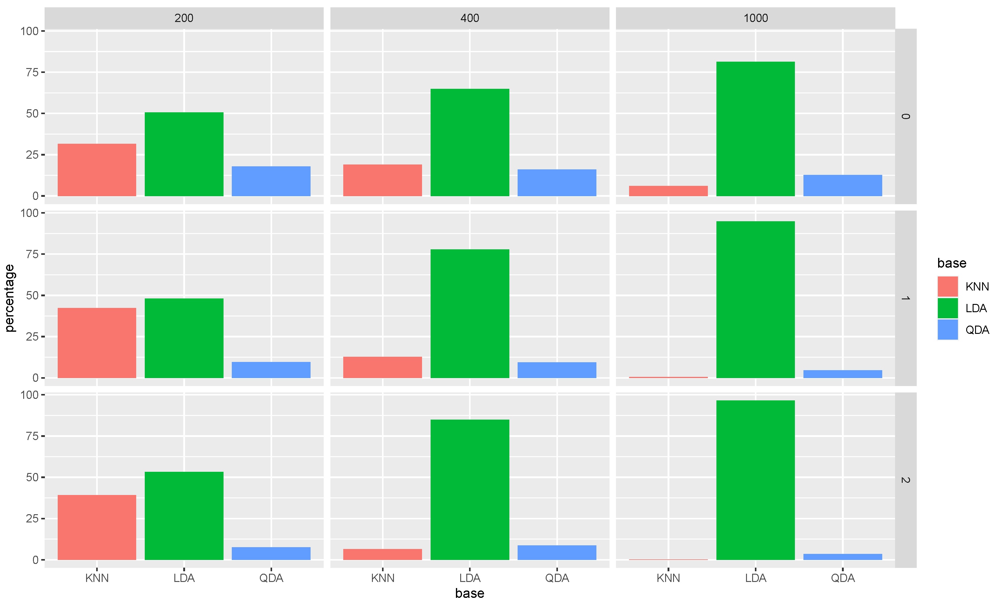
Let us take a look at Figure 1. The first row shows the bar charts for the selection percentage of each base classifier in the Super RaSE algorithm among the 200 repetitions when the sample size n varies in $\{200,400,1000\}$. It shows that when $n=200$, the percentage of LDA is around 50%. As the sample size increases, the percentage of LDA also increases, showing that having a larger sample size helps us to select the model from which the data are generated.

Now, let us look at the column of $n=1000$; we can see that as the iteration process moves on, the percentage of LDA is increasing as well, leading to almost 100% for SRaSE${}_2$.

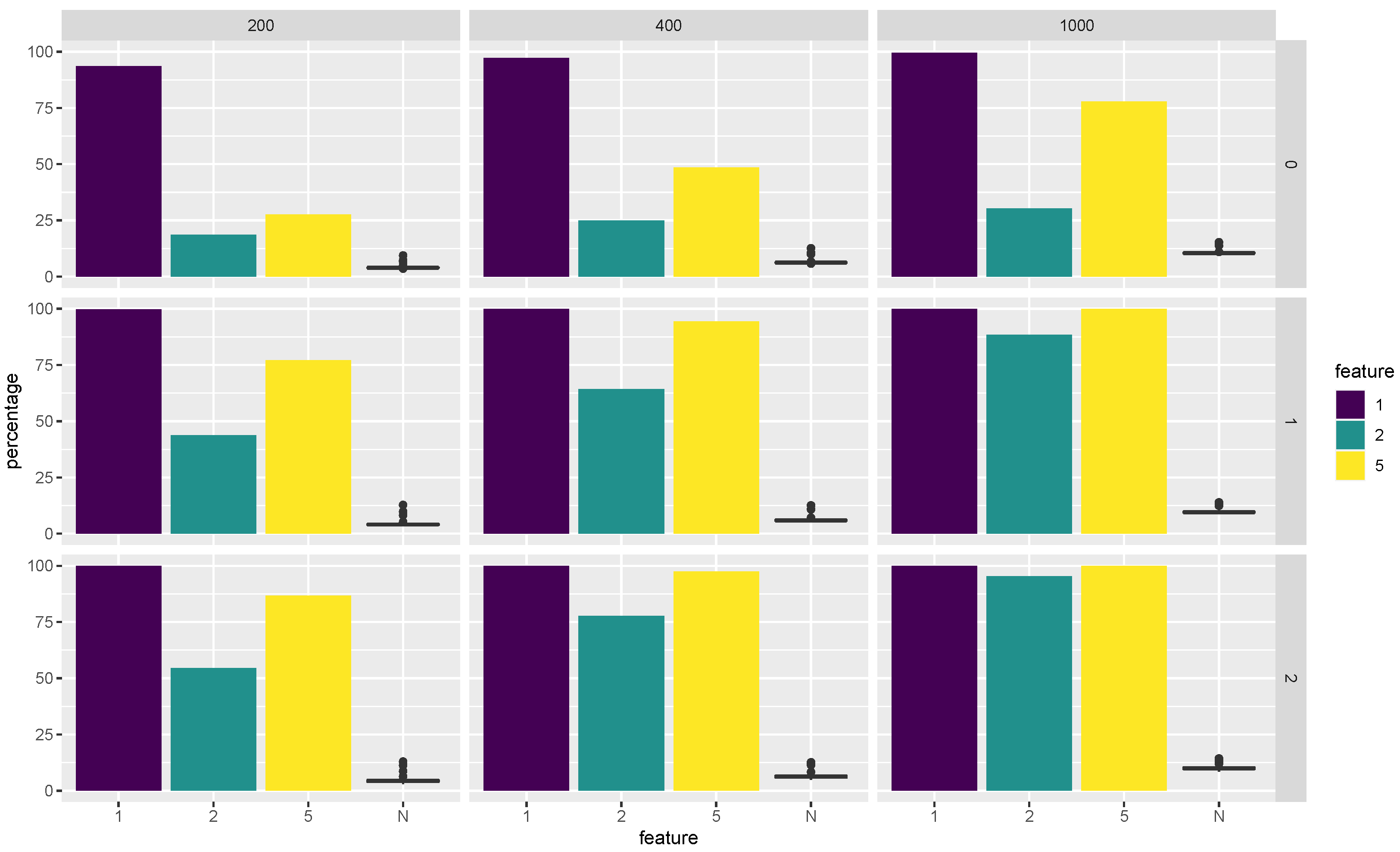
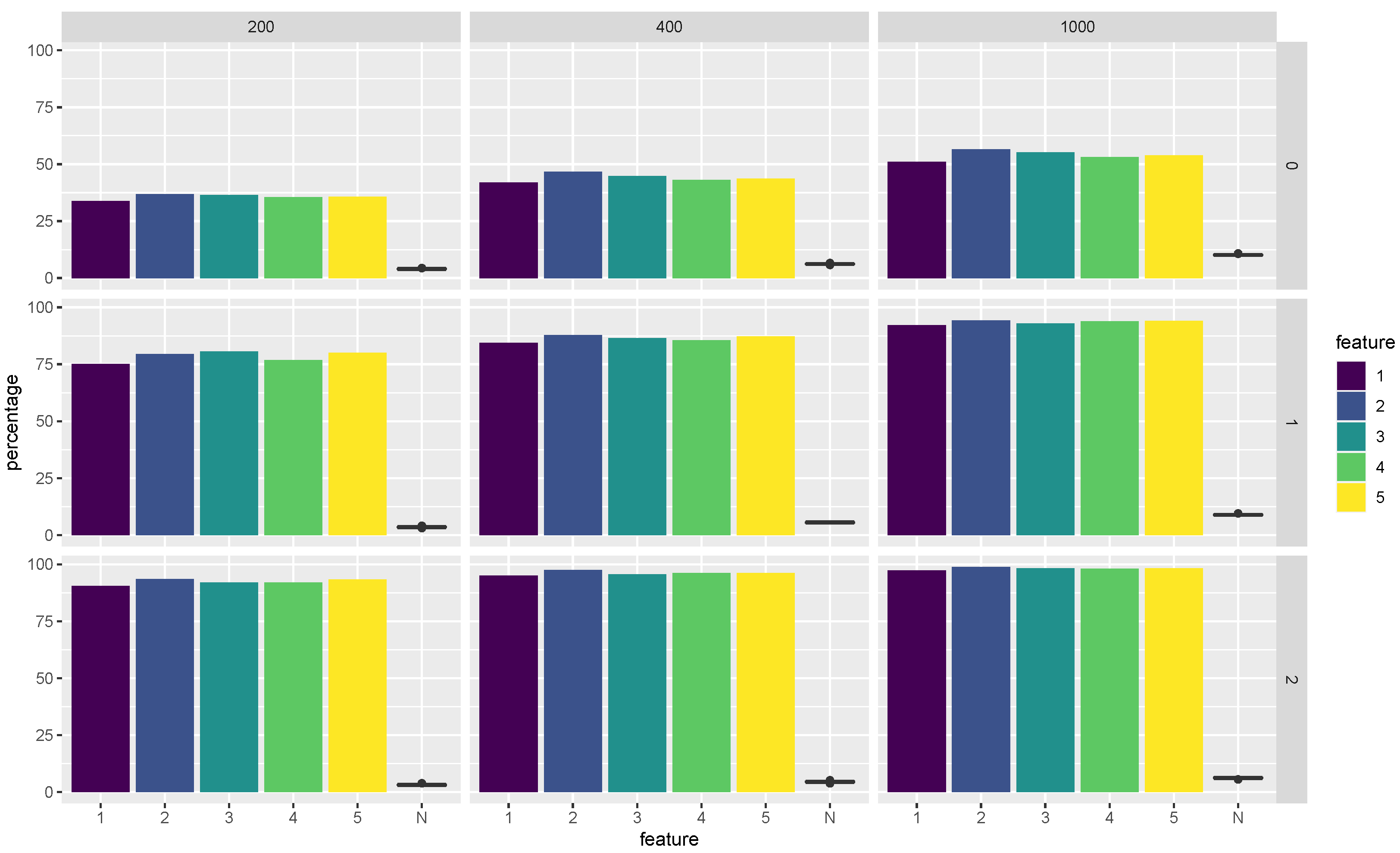
The second product of the Super RaSE algorithm and its iterative version is the selected frequencies for each feature among the weaker learner with a particular classifier. Figure 2 visualizes the selected proportions of features among all the $B_1$ classifiers that use LDA as the base classifier. In particular, we show the selected proportions for each feature in the minimum discriminative set $S^{*}=\{1,2,5\}$. In the same figure, we also show a boxplot of the selected proportion of all the noisy features as a way to verify whether the Super RaSE algorithms can distinguish the important features from the noisy features.

From Figure 2, we observe that when $n=200$, the vanilla Super RaSE algorithm does not select the important variables 2 and 5 with a high percentage. However, the iteration greatly helps the algorithm to increase the selected percentages for features 2 and 5. In addition, the increase in sample size leads to the selection of all important features with almost 100% percentage. It is also worth noting that the noise features all have a relatively small selection frequency, showing the power of feature ranking in the Super RaSE algorithms. Similar figures can also be generated for the selected proportions of features among the $B_1$ classifiers that use QDA and KNN as the base classifier, respectively. For simplicity, we omit these figures in our presentation.

3.2. Model 2: QDA

Now, we consider the case where the data are generated from a sparse QDA model with the following setting (Fan et al. 2015; Tian and Feng 2021b).

$\mathit{x}|y=r\sim N({\mathsf{\mu }}^{\left(r\right)},{\mathsf{\Sigma }}^{\left(r\right)}),r=0,1$, where ${\mathsf{\Omega }}^{\left(0\right)}={\left({\mathsf{\Sigma }}^{\left(0\right)}\right)}^{-1}$ is a $p\times p$ banded matrix with ${\left({\mathsf{\Omega }}^{\left(0\right)}\right)}_{ii}=1$ and ${\left({\mathsf{\Omega }}^{\left(0\right)}\right)}_{ik}=0.3$ for $|i-k|=1$ and all other entries zero. The inverse covariance matrix for class 1 is ${\mathsf{\Omega }}^{\left(1\right)}={\mathsf{\Omega }}^{\left(0\right)}+\mathsf{\Omega }$, where $\mathsf{\Omega }$ is a $p\times p$ sparse symmetric matrix with ${\mathsf{\Omega }}_{10,10}=-0.3758,{\mathsf{\Omega }}_{10,30}=0.0616,{\mathsf{\Omega }}_{10,50}=0.2037,{\mathsf{\Omega }}_{30,30}=-0.5482,$${\mathsf{\Omega }}_{30,50}=0.0286,{\mathsf{\Omega }}_{50,50}=-0.4614$ and all other entries zero. The dimension is $p=200$ and we again vary the sample size $n\in \{200,400,1000\}$.

We can easily verify that the feature subset $\{1,2,10,30,50\}$ is the minimal discriminative set $S^{*}$. In

Table 2. Summary of test classification error rates for each classifier under various sample sizes over 200 repetitions in Model 2 (QDA). The results are presented as mean values with the standard deviation values in parentheses. Here, the best performing method in each column is highlighted in bold and the methods that are within one standard deviation away are highlighted in italic.

	$\mathit{n}=200$	$\mathit{n}=400$	$\mathit{n}=1000$
SRaSE	30.82(3.29)	28.68(3.23)	26.12(2.66)
SRaSE${}_1$	27.58(2.33)	24.64(1.85)	23.03(1.38)
SRaSE${}_2$	27.36(2.67)	24.04(1.74)	22.63(1.41)
RaSE-LDA	37.3(3.17)	36.11(1.97)	35.67(1.73)
RaSE-QDA	32.52(2.90)	30.44(2.60)	29(1.97)
RaSE-KNN	31.1(3.23)	27.83(2.41)	25.22(1.56)
RaSE${}_1$-LDA	36.09(2.87)	32.82(1.74)	32.68(1.49)
RaSE${}_1$-QDA	26.83(2.47)	25.07(1.89)	23.53(1.50)
RaSE${}_1$-KNN	28.76(2.60)	25.88(1.98)	24.18(1.47)
RaSE${}_2$-LDA	38.09(2.48)	33.69(1.83)	32.71(1.55)
RaSE${}_2$-QDA	26.99(2.68)	24.87(1.99)	23.11(1.60)
RaSE${}_2$-KNN	28.73(2.56)	25.46(1.82)	23.76(1.54)
LDA	49.03(1.94)	42.88(1.82)	38.68(1.70)
QDA	NA	NA	45.13(1.58)
KNN	45.67(1.78)	44.63(2.02)	43.43(1.63)
RF	37.34(2.91)	31.61(2.19)	27.42(1.60)

, we present the performance of different methods for Model 2 under different sample sizes.

From the table, when $n=400$ and $n=1000$, SRaSE${}_2$ is the best performing method, achieving the smallest test classification error. When $n=200$, SRaSE${}_2$ is within one standard error away from the optimal method. This result is very encouraging in the sense that Super RaSE could improve the performance of the original RaSE coupled with the true model from which the data are generated. This shows that the Super RaSE algorithms are extremely robust and avoid the need to choose a base classifier as needed in the original RaSE algorithm.

As in Model 1, we again present the average selected proportion of each base classifier in Figure 3 as well as the average selected proportion of each feature among the $B_1$ weak learners with the chosen base classifier being QDA in Figure 4. In Figure 4, we also show a boxplot of the selected proportion of all the noisy features.

In Figure 3, we again observe that as we iterate the Super RaSE algorithm, the proportion of QDA greatly increases, reaching almost 100 percent for RaSE${}_2$ over all sample sizes. This shows that the iterative Super RaSE algorithm is able to identify the true model.

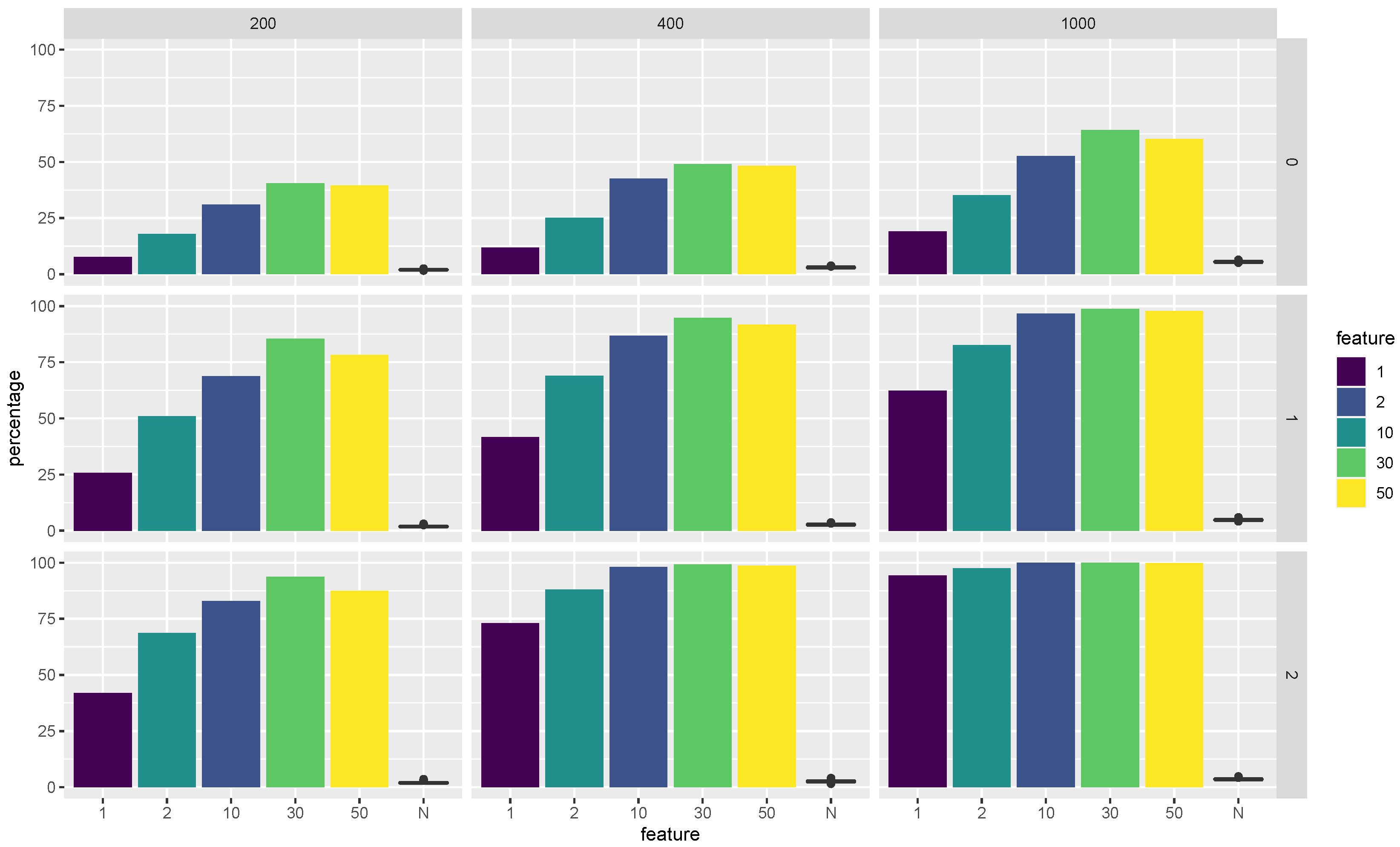
In Figure 4, we can observe that the average selected proportions of each important feature are pretty high, showing that the Super RaSE is able to pick up the important features. In particular, when $n=1000$, the iteration helps all the features to have a higher selected proportion, reaching nearly 100 percent for SRaSE${}_2$.

3.3. Model 3: KNN

Having considered two parametric models, let us move to an example where the label is generated in a non-parametric way (Tian and Feng 2021b). We will be following the idea of nearest neighbors when assigning the labels.

The detailed data generation process is as follows. First, 10 initial points ${\mathit{z}}_1,\cdots ,{\mathit{z}}_{10}$ are generated i.i.d. from $N({\mathbf{0}}_{p\times 1},I_p)$. Out of the 10 points, 5 are labeled as 0 and the other 5 are labeled as 1. Then, each observation $(\mathit{x},y)$ pair is generated as follows. First, we randomly select one element from $\{{\mathit{z}}_1,\cdots ,{\mathit{z}}_{10}\}$. Let us suppose it is ${\mathit{z}}_{k_i}$, corresponding to the i-th observation. Then, the corresponding $y_i$ will take the label as ${\mathit{z}}_{k_1}$, and the feature vector ${\mathit{x}}_i$ is generated as ${\mathit{x}}_i\sim N({({\mathbf{z}}_{k_i,S^{*}}^T,{\mathbf{0}}_{1\times (p-5)})}^T,0.5^2{I}_p)$. The general idea is that we are generating a mixture of 10 Gaussian clusters that surround each of the $\{{\mathit{z}}_1,\cdots ,{\mathit{z}}_{10}\}$ when they are embedded in a p-dimensional space.

From the data generation process, the minimal discriminative set is $S^{*}=\{1,2,3,4,5\}$. We consider $p=200$, and $n\in \{200,400,1000\}$. The summary of the test classification error rates over 200 repetitions is presented in

Table 3. Summary of test classification error rates for each classifier under various sample sizes over 200 repetitions in Model 3 (KNN). The results are presented as mean values with the standard deviation values in parentheses. Here, the best performing method in each column is highlighted in bold and the methods that are within one standard deviation away are highlighted in italic.

	$\mathit{n}=200$	$\mathit{n}=400$	$\mathit{n}=1000$
SRaSE	16.89(6.10)	13.54(5.39)	10.68(4.74)
SRaSE${}_1$	8.18(4.18)	6.86(3.58)	6.12(3.24)
SRaSE${}_2$	7.22(3.82)	6.39(3.42)	5.78(3.09)
RaSE-LDA	27.38(9.53)	25.08(8.40)	24.92(9.05)
RaSE-QDA	24.24(7.20)	22.62(6.77)	22.04(6.73)
RaSE-KNN	13.26(5.03)	10.67(4.44)	8.85(4.05)
RaSE${}_1$-LDA	25.89(10.13)	23.05(8.49)	23.42(8.95)
RaSE${}_1$-QDA	13.83(5.88)	12.54(5.79)	12.7(5.51)
RaSE${}_1$-KNN	7.51(3.80)	6.16(3.48)	5.9(3.12)
RaSE${}_2$-LDA	27.49(10.13)	23.39(8.51)	23.39(9.05)
RaSE${}_2$-QDA	13.15(5.00)	11.9(5.38)	12.15(5.22)
RaSE${}_2$-KNN	7.06(3.62)	5.89(3.32)	5.74(3.02)
LDA	47.51(2.66)	33.27(7.65)	27.89(8.97)
QDA	NA	NA	36.7(4.83)
KNN	24.49(6.64)	21.04(6.60)	19.07(6.50)
RF	23.64(8.05)	17.39(6.19)	14.84(5.73)

.

From Table 3, we can see that Super RaSE and its iterative versions still have very competitive performance compared with other methods. In particular, both SRaSE${}_1$ and SRaSE${}_2$ reach test errors that are within one standard deviation of the best performing method RaSE${}_2$-KNN, which uses the knowledge of the data generation process. As a method-free algorithm, Super RaSE algorithms and their iterative versions are very appealing, having similar performance as the best-performing ones without the need to specify which base classifier to use.

Similar to Models 1 and 2, we again present the average selected proportion of each base method in Figure 5. Figure 6 visualizes the selected proportions of features among all the $B_1$ classifiers that use KNN as the base classifier. In addition to the bar chart for the average selected proportion of each important feature, Figure 6 also includes a boxplot of the selected proportion of all the noisy features.

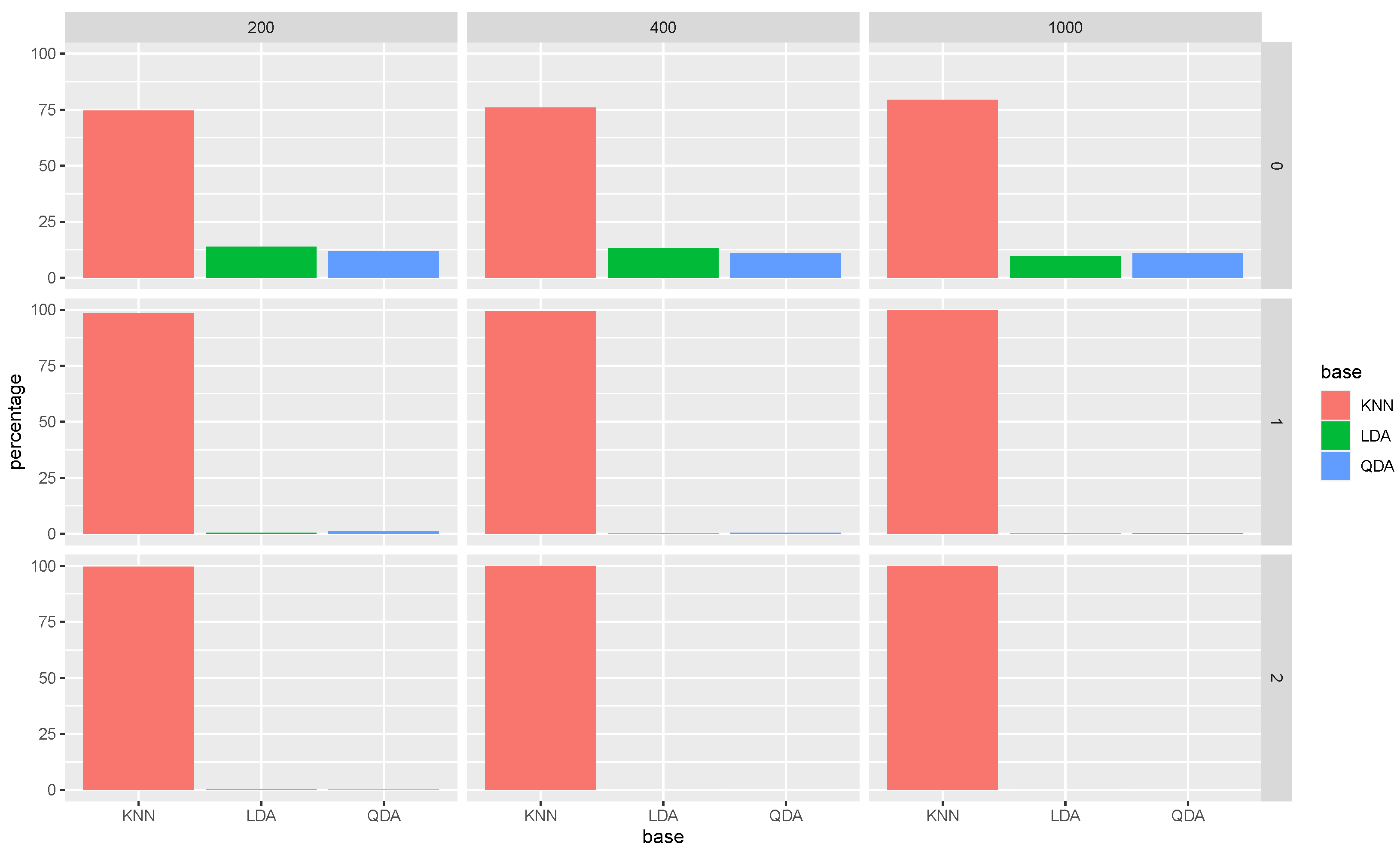
In Figure 5, we have a similar story as Figure 1 and Figure 3. We can see that the average selection percentage of KNN is almost 100 percent for both SRaSE${}_1$ and SRaSE${}_2$, showing that one step iteration is enough to almost always find the best classifier for this particular model.

In Figure 6, we can see that without iteration, Super RaSE, on average, only selects the five important features with around 50 percent out of the 200 repetitions. With the help of iterations, the percentages of all five important features increase substantially, to almost 100 percent when $n=1000$. This experiment shows the merit of iterative Super RaSE in terms of capturing the important features.

4. Real Data Analysis

In this section, we evaluate the proposed Super RaSE algorithm and its iterative version via two real data examples. Here, we compare SRaSE and SRaSE${}_1$ with the original RaSE with the base classifiers LDA, QDA, KNN along with their one-step iterated versions. We also add the classic LDA, QDA, KNN, and random forest (RF) to the horse race. Same as in the simulation studies, we use the default values for all parameters in the Super RaSE algorithm and its iterative version ($B_1=200$, $B_2=500$).

4.1. Mice Protein Expression

The first example we consider is the mice protein expression data set (Higuera et al. 2015). The data set is publicly available at https://archive.ics.uci.edu/ml/datasets/Mice+Protein+Expression (accessed on 27 September 2020). There are 1080 mice in total, with 570 healthy mice (class 0) and 510 with Down’s syndrome (class 1). A total of 77 features are measured, representing the expression of 77 different proteins. Here, we vary the size of the training sample in $\{200,500,800\}$, and the remaining mice are set as the test data.

The average of test misclassification rates and standard deviations of 200 replicates are calculated with the results reported in

Table 4. Summary of test classification error rates for each classifier under various sample sizes over 200 repetitions for the mice protein expression data set. The results are presented as mean values with the standard deviation values in parentheses. Here, the best performing method in each column is highlighted in bold and the methods that are within one standard deviation away are highlighted in italic.

	$\mathit{n}=200$	$\mathit{n}=500$	$\mathit{n}=800$
SRaSE	7.08(1.92)	3.33(2.54)	0.67(0.65)
SRaSE${}_1$	6.76(1.95)	2.56(2.39)	0.65(0.60)
RaSE-LDA	7.41(1.14)	5.7(0.93)	4.65(1.24)
RaSE-QDA	9.14(2.58)	4.81(1.17)	3.44(1.23)
RaSE-KNN	6.8(1.88)	1.55(0.88)	0.62(0.55)
RaSE${}_1$-LDA	7.24(1.10)	5.53(1.02)	4.49(1.23)
RaSE${}_1$-QDA	9.38(2.21)	5.16(1.16)	3.4(1.16)
RaSE${}_1$-KNN	7.43(2.00)	1.7(0.87)	0.6(0.56)
LDA	7.07(1.37)	3.88(0.85)	3.13(1.08)
KNN	20.53(2.47)	7.75(1.44)	2.8(1.21)
RF	8.32(1.71)	2.62(0.94)	1.04(0.73)

. When $n=200$, our newly proposed algorithm SRaSE${}_1$ achieves the lowest error among all approaches. When $n=1000$, both SRaSE and SRaSE${}_1$ are within one standard deviation from the best performing method: RaSE${}_1$-KNN. This shows that Super RaSE and its iterative versions are very accurate in terms of prediction performance.

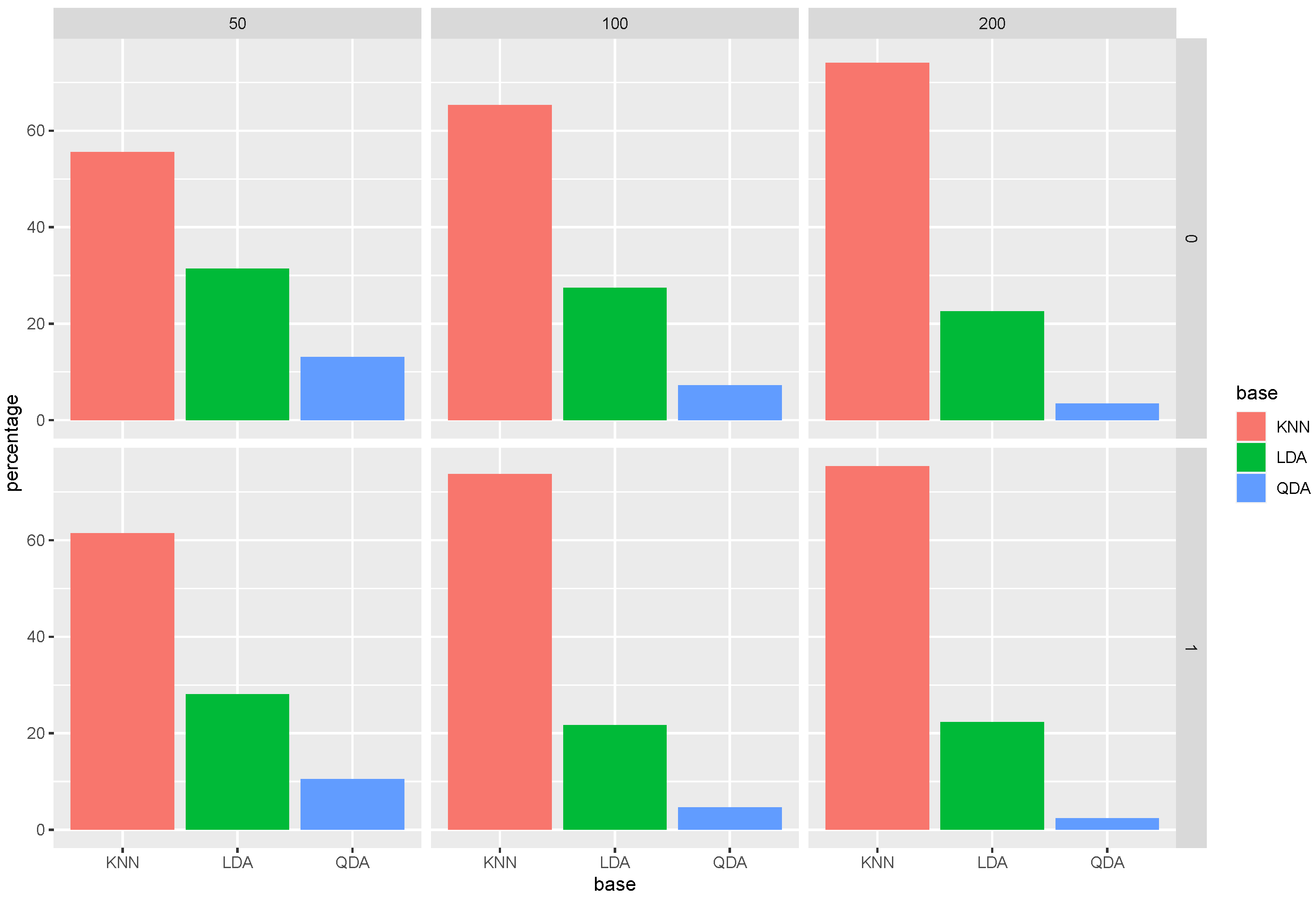
Next, we show the average selected proportion for each base method for different sample sizes and iteration numbers in Figure 7.

From this figure, we observe a very interesting phenomenon. That is when $n=200$, the selected proportion of LDA is the highest (over 75%). This choice is very reasonable since comparing the RaSE classifier with different base classifiers, RaSE${}_1$-LDA has the best performance among RaSE${}_1$ combined with other base classifiers. Now, looking at the case when $n=800$, our Super RaSE and SRaSE${}_1$ both select KNN over 95% percent of the time. Again, let us look at the RaSE classifier with a fixed base classifier; it is easy to observe from Table 4 that RaSE${}_1$-KNN has a much better performance than both RaSE${}_1$-LDA and RaSE${}_1$-QDA. This shows that the Super RaSE algorithm is very adaptive to the specific scenario in the sense that in each of the $B_1$ weak learners, it automatically selects the base classifier among the randomly selected $B_2$ classifiers coupled with the random subspaces.

4.2. Hand-Written Digits Recognition

The second data set we consider is the hand-written digits recognition data set that consists of features of hand-written numerals (0–9) extracted from a collection of Dutch utility maps (Dua and Graff 2019). The data set is publicly available at https://archive.ics.uci.edu/ml/datasets/Multiple+Features (accessed on 27 September 2020). Out of the 10 digits, we focus the observations corresponding to numbers 7 (class 0) and 9 (class 1). After this preprocessing, we have 400 numbers, with 200 in class 0 and another 200 in class 1. We again vary the training sample size, this time in $\{50,100,200\}$. The rest of the observations are used as the test data. The average of the test misclassification rates along with their standard deviations are reported in

Table 5. Summary of test classification error rates for each classifier under various sample sizes over 200 repetitions for the hand-written digits recognition data set. The results are presented as mean values with the standard deviation values in parentheses. Here, the best performing method in each column is highlighted in bold and the methods that are within one standard deviation away are highlighted in italic.

	$\mathit{n}=50$	$\mathit{n}=100$	$\mathit{n}=200$
SRaSE	2(1.06)	1.2(0.65)	0.78(0.48)
SRaSE${}_1$	1.78(1.03)	1.04(0.57)	0.62(0.37)
RaSE-LDA	1.56(0.85)	1.13(0.59)	0.8(0.54)
RaSE-QDA	2.5(1.47)	1.89(0.91)	1.47(0.96)
RaSE-KNN	1.86(0.96)	1.12(0.66)	0.75(0.45)
RaSE${}_1$-LDA	1.06(0.63)	0.7(0.35)	0.53(0.40)
RaSE${}_1$-QDA	2.18(1.66)	1.18(0.71)	0.85(0.61)
RaSE${}_1$-KNN	1.72(0.95)	1.02(0.62)	0.6(0.44)
LDA	NA	1.82(0.96)	1.01(0.56)
QDA	NA	NA	3.25(2.32)
KNN	1.42(1.32)	0.67(0.41)	0.6(0.47)
RF	2.34(1.24)	1.63(0.73)	1.37(0.74)

.

From Table 5, we can see that the Super RaSE and its iterative versions still have competitive performance, especially when $n=100$ and $n=200$. SRaSE${}_1$ has a very similar performance as the best performing method when $n=100$ and $n=200$. Having a careful look, it is interesting to observe that SRaSE${}_1$ closely mimics the performance of RaSE${}_1$-KNN, leading us to wonder whether KNN is the most selected base method among the $B_1$ classifiers. We confirm that this is the case by presenting the average selected proportion of each base classifier for SRaSE and SRaSE${}_1$ in Figure 8.

From Figure 8, we can see that KNN is indeed the most selected base classifier across all scenarios, with its selected proportion being almost 100% when $n=200$.

5. Discussion

In this work, motivated by the random subspace ensemble (RaSE) classification, we propose a new ensemble classification framework, named Super RaSE, which is a completely model-free approach. While RaSE has to be paired with a single base classifier, Super RaSE can work with a collection of base classifiers, making it more flexible and robust in applications. In particular, we recommend that the practitioners include several different base classifiers, including parametric and non-parametric ones, so as to make the Super RaSE framework more powerful. It is worth noting that as we include more base classifiers in the Super RaSE algorithm, perhaps larger values of $B_1$ and $B_2$ are needed so as to generate a sufficient number of random subspace and base classifier pairs among the $B_2$ classifiers, and reach a more stable result with a larger $B_1$. By randomly generating the pair of base classifier and subspace, it will automatically select a collection of good base classifier and subspace pairs. Besides the superb prediction performance on the test data, the Super RaSE algorithms also provide two important by-products. The first one is a quality measure of each base classifier, which can provide insight as to which base classifiers are more appropriate for the given data. The second by-product is that, given each base classifier, the Super RaSE will also generate an important measure for each feature, which can be used for feature screening and ranking (Fan et al. 2011; Saldana and Feng 2018; Yousuf and Feng 2021), just like the original RaSE (Tian and Feng 2021a). The feature important measure can provide an interpretable machine learning model, which is very useful in understanding how the method works.

There are many possible future research directions. First, this paper only considers the binary classification problem, but there may be more than two classes in applications. How to extend the Super RaSE algorithm to the multiclass situation is an important topic. In particular, we need to find multiclass classification algorithms as well as a new decision function when we ensemble the $B_1$ weak learners. In particular, the original thresholding step in line 9 of Algorithm 1 is no longer applicable. Second, in addition to the classification problem, it is also worthwhile to study the corresponding algorithm under a regression setting. To achieve this, we can change the prediction step from thresholding to a simple averaging. Third, using the selected proportion of features, it is possible to develop a variable selection or variable screening algorithm. For example, we can set a threshold for variable screening which is expected to capture important interaction effects in addition to the marginal ones. The interaction detection problem has been well studied in high-dimensional quadratic regression (Hao et al. 2018). However, the Super RaSE will greatly expand the scope within which the interaction selection works, allowing for the interaction among features to be of different formats. Lastly, in both RaSE and Super RaSE, we use all the observations in each combination of the base classifier and a random subspace. We know that random forest is viewed as a very robust classifier, partly due to the fact that it uses a bagging sample (Breiman 1996) for each tree during the ensemble process. This particular bagging step makes the trees uncorrected, which reduces the variable of the final classifier. A natural extension of Super RaSE is Bagging Super RaSE, which uses a bagging sample for each of the $B_1$ groups. It is worth noting that it may not be a good idea to use a different bagging sample for each of the $B_2$ pairs of a base classifier and an associated random subspace, due to the fact that it could lead to an unfair comparison among the $B_2$ pairs.

References

- Blaser, Rico, and Piotr Fryzlewicz. 2016. Random rotation ensembles. The Journal of Machine Learning Research 17: 126–51. [Google Scholar]
- Breiman, Leo. 1996. Bagging predictors. Machine Learning 24: 123–40. [Google Scholar] [CrossRef] [Green Version]
- Breiman, Leo. 2001. Random forests. Machine Learning 45: 5–32. [Google Scholar] [CrossRef] [Green Version]
- Breiman, Leo, Jerome H. Friedman, Richard A. Olshen, and Charles J. Stone. 2017. Classification and Regression Trees. Boca Raton: Routledge. [Google Scholar]
- Cannings, Timothy I., and Richard J. Samworth. 2017. Random-projection ensemble classification. Journal of the Royal Statistical Society: Series B (Statistical Methodology) 79: 959–1035. [Google Scholar] [CrossRef]
- Dainotti, Alberto, Antonio Pescape, and Kimberly C. Claffy. 2012. Issues and future directions in traffic classification. IEEE Network 26: 35–40. [Google Scholar] [CrossRef] [Green Version]
- Dietterich, Thomas G. 2000. Ensemble methods in machine learning. In International Workshop on Multiple Classifier Systems. New York: Springer, pp. 1–15. [Google Scholar]
- Dua, Dheeru, and Casey Graff. 2019. Uci Machine Learning Repository. Irvine: School of Information and Computer Science, University of California. [Google Scholar]
- Durrant, Robert J., and Ata Kabán. 2015. Random projections as regularizers: Learning a linear discriminant from fewer observations than dimensions. Machine Learning 99: 257–86. [Google Scholar] [CrossRef] [Green Version]
- Dvorsky, Jan, Jaroslav Belas, Beata Gavurova, and Tomas Brabenec. 2021. Business risk management in the context of small and medium-sized enterprises. Economic Research-Ekonomska Istraživanja 34: 1690–708. [Google Scholar] [CrossRef]
- Fan, Jianqing, Yang Feng, Jiancheng Jiang, and Xin Tong. 2016. Feature augmentation via nonparametrics and selection (fans) in high-dimensional classification. Journal of the American Statistical Association 111: 275–87. [Google Scholar] [CrossRef] [PubMed]
- Fan, Jianqing, Yang Feng, and Rui Song. 2011. Nonparametric independence screening in sparse ultra-high-dimensional additive models. Journal of the American Statistical Association 106: 544–57. [Google Scholar] [CrossRef] [Green Version]
- Fan, Jianqing, Yang Feng, and Xin Tong. 2012. A road to classification in high dimensional space: The regularized optimal affine discriminant. Journal of the Royal Statistical Society: Series B (Statistical Methodology) 74: 745–71. [Google Scholar] [CrossRef]
- Fan, Yingying, Yinfei Kong, Daoji Li, and Zemin Zheng. 2015. Innovated interaction screening for high-dimensional nonlinear classification. The Annals of Statistics 43: 1243–72. [Google Scholar] [CrossRef]
- Feng, Yang, and Qingfeng Liu. 2020. Nested model averaging on solution path for high-dimensional linear regression. Stat 9: e317. [Google Scholar] [CrossRef]
- Feng, Yang, Qingfeng Liu, Qingsong Yao, and Guoqing Zhao. 2021a. Model averaging for nonlinear regression models. Journal of Business & Economic Statistics, 1–14. [Google Scholar] [CrossRef]
- Feng, Yang, Xin Tong, and Weining Xin. 2021b. Targeted Crisis Risk Control: A Neyman-Pearson Approach. Available online: https://papers.ssrn.com/sol3/papers.cfm?abstract_id=3945980 (accessed on 27 September 2020).
- Fix, Evelyn, and Joseph Lawson Hodges. 1989. Discriminatory analysis. nonparametric discrimination: Consistency properties. International Statistical Review/Revue Internationale de Statistique 57: 238–47. [Google Scholar] [CrossRef]
- Gao, Xiaoli, S. E. Ahmed, and Yang Feng. 2017. Post selection shrinkage estimation for high-dimensional data analysis. Applied Stochastic Models in Business and Industry 33: 97–120. [Google Scholar] [CrossRef] [Green Version]
- Hao, Ning, Yang Feng, and Hao Helen Zhang. 2018. Model selection for high-dimensional quadratic regression via regularization. Journal of the American Statistical Association 113: 615–25. [Google Scholar] [CrossRef] [Green Version]
- Higuera, Clara, Katheleen J. Gardiner, and Krzysztof J. Cios. 2015. Self-organizing feature maps identify proteins critical to learning in a mouse model of down syndrome. PLoS ONE 10: e0129126. [Google Scholar] [CrossRef]
- Ho, Tin Kam. 1998. The random subspace method for constructing decision forests. IEEE Transactions on Pattern Analysis and Machine Intelligence 20: 832–44. [Google Scholar]
- Jurgovsky, Johannes, Michael Granitzer, Konstantin Ziegler, Sylvie Calabretto, Pierre-Edouard Portier, Liyun He-Guelton, and Olivier Caelen. 2018. Sequence classification for credit-card fraud detection. Expert Systems with Applications 100: 234–45. [Google Scholar] [CrossRef]
- Kotsiantis, Sotiris B., I. Zaharakis, and P. Pintelas. 2007. Supervised machine learning: A review of classification techniques. Emerging Artificial Intelligence Applications in Computer Engineering 160: 3–24. [Google Scholar]
- Mai, Qing, Hui Zou, and Ming Yuan. 2012. A direct approach to sparse discriminant analysis in ultra-high dimensions. Biometrika 99: 29–42. [Google Scholar] [CrossRef]
- Michalski, Grzegorz, Małgorzata Rutkowska-Podołowska, and Adam Sulich. 2018. Remodeling of fliem: The cash management in polish small and medium firms with full operating cycle in various business environments. In Efficiency in Business and Economics. Berlin/Heidelberg: Springer, pp. 119–32. [Google Scholar]
- Raftery, Adrian E., David Madigan, and Jennifer A. Hoeting. 1997. Bayesian model averaging for linear regression models. Journal of the American Statistical Association 92: 179–91. [Google Scholar] [CrossRef]
- Rokach, Lior. 2010. Ensemble-based classifiers. Artificial Intelligence Review 33: 1–39. [Google Scholar] [CrossRef]
- Saldana, Diego Franco, and Yang Feng. 2018. Sis: An r package for sure independence screening in ultrahigh-dimensional statistical models. Journal of Statistical Software 83: 1–25. [Google Scholar] [CrossRef] [Green Version]
- Steinwart, Ingo, and Andreas Christmann. 2008. Support Vector Machines. Berlin/Heidelberg: Springer Science & Business Media. [Google Scholar]
- Szczygieł, N., M. Rutkowska-Podolska, and Grzegorz Michalski. 2014. Information and communication technologies in healthcare: Still innovation or reality? Innovative and entrepreneurial value-creating approach in healthcare management. Paper presented at the 5th Central European Conference in Regional Science, Košice, Slovakia, October 5–8; pp. 1020–29. [Google Scholar]
- Tian, Ye, and Yang Feng. 2021a. Rase: A variable screening framework via random subspace ensembles. Journal of the American Statistical Association, 1–30, accepted. [Google Scholar] [CrossRef]
- Tian, Ye, and Yang Feng. 2021b. Rase: Random subspace ensemble classification. J. Mach. Learn. Res. 22: 1–93. [Google Scholar]
- Tong, Xin, Yang Feng, and Jingyi Jessica Li. 2018. Neyman-pearson classification algorithms and np receiver operating characteristics. Science Advances 4: eaao1659. [Google Scholar] [CrossRef] [Green Version]
- Van der Laan, Mark J., Eric C. Polley, and Alan E. Hubbard. 2007. Super learner. Statistical Applications in Genetics and Molecular Biology 6. [Google Scholar] [CrossRef] [PubMed]
- Yousuf, Kashif, and Yang Feng. 2021. Targeting predictors via partial distance correlation with applications to financial forecasting. Journal of Business & Economic Statistics, 1–13. [Google Scholar] [CrossRef]
Figure 1.
The average selected proportion for each base method for different sample sizes (corresponding to each column) and iteration number (corresponding to each row) in Model 1 (LDA).
Figure 2.
The average selected proportion for each feature for different sample sizes (corresponding to each column) and iteration number (corresponding to each row) in Model 1 (LDA).
Figure 3.
The average selected proportion for each base method for different sample sizes (corresponding to each column) and iteration number (corresponding to each row) in Model 2 (QDA).
Figure 4.
The average selected proportion for each feature for different sample size (corresponding to each column) and iteration number (corresponding to each row) in Model 2 (QDA).
Figure 5.
The average selected proportion for each base method for different sample sizes (corresponding to each column) and iteration number (corresponding to each row) in Model 3 (KNN).
Figure 6.
The average selected proportion for each feature for different sample sizes (corresponding to each column) and iteration number (corresponding to each row) in Model 3 (KNN).
Figure 7.
The average selected proportion for each base method for different sample sizes (corresponding to each column) and iteration number (corresponding to each row) for the mice protein expression data.
Figure 8.
The average selected proportion for each base method for different sample sizes (corresponding to each column) and iteration number (corresponding to each row) for the hand-written digits recognition data.