
Neural Network Based Deep Learning Method for Multi-Dimensional Neutron Diffusion Problems with Novel Treatment to Boundary


1
Sino-French Institute of Nuclear Engineering and Technology, Sun Yat-Sen University, Zhuhai 519082, China
2
Department of Mechanical and Nuclear Engineering, Virginia Commonwealth University, Richmond, VA 23284-3015, USA
*
Authors to whom correspondence should be addressed.
J. Nucl. Eng. 2021, 2(4), 533-552; https://doi.org/10.3390/jne2040036
Submission received: 8 October 2021
/
Revised: 15 November 2021
/
Accepted: 1 December 2021
/
Published: 9 December 2021
Abstract
:In this paper, the artificial neural networks (ANN) based deep learning (DL) techniques were developed to solve the neutron diffusion problems for the continuous neutron flux distribution without domain discretization in advance. Due to its mesh-free property, the DL solution can easily be extended to complicated geometries. Two specific realizations of DL methods with different boundary treatments are developed and compared for accuracy and efficiency, including the boundary independent method (BIM) and boundary dependent method (BDM). The performance comparison on analytic benchmark indicates BDM being the preferred DL method. Novel constructions of trial function are proposed to generalize the application of BDM. For a more in-depth understanding of the BDM on diffusion problems, the influence of important hyper-parameters is further investigated. Numerical results indicate that the accuracy of BDM can reach hundreds of times higher than that of BIM on diffusion problems. This work can provide a new perspective for applying the DL method to nuclear reactor calculations.
1. Introduction
Neutron diffusion equation, as a simplified form with the P1 approximation of neutron transport equation [1,2], is commonly used in reactor core calculations for nuclear reactor design and analysis. Focusing on solving neutron diffusion equation, many mesh-based numerical methods have been proposed and employed by various groups. These methods discretize the calculation domain into many subdomains via different numerical techniques, including the finite element method (FEM) [3], the finite volume method (FVM) [4] and the finite difference method (FDM) [5,6]. The pros and cons of these mesh-based methods are generally recognized and the accuracy of these methods is essentially limited by the number of nodes and the geometric shape of the problem under investigated [7]. In particular, these mesh-based methods can only obtain discrete solutions associated with the discretized nodes. When using these discrete solutions for other purposes, such as for the calculation of group constants or k-eigenvalue in reactor problems, numerical integrals of these discrete solutions are indispensable. The error caused by the numerical integral is limited by the complexity of the mesh structure, and thus is very hard to reduce. As a result, a mesh independent and easy implemented computational method is more desired for problems with complex geometries.
The deep learning (DL) method, due to its powerful ability to discover complex structures in large data set and its low human intervene requirements, has attracted many attentions for engineering problems in recent years [8,9,10,11,12]. The DL method has produced encouraging results in many applications of various disciplines, including language processing [13,14,15,16], image recognition [17,18,19], speech recognition [20,21] and finance [22]. In recent years, the DL method has been extended to the field of nuclear reactor engineering by some researchers and achieved good performance [23,24,25]. However, the traditional DL method usually needs a large amount of data to train the deep network, whereas nuclear engineering applications always lack of the training data since experimental data of nuclear engineering are normally difficult to obtain and collecting computational data are usually time-consuming.
To improve this condition, the physics-informed DL (PIDL) method is proposed. This method constructs the loss function by using the partial differential equation (PDE) as regulation term rather than using the large amount of data like classical DL method. Owning to this advantage, the PIDL can be applied to solve the PDE based physics problems with limited or even no data available [26,27,28]. In comparing with the classical method, such as the FEM, the PIDL shows some outstanding advantages. Since the PIDL doesn’t require mesh discretization, this method has strong geometry adaptability and can directly provide continuous solutions over whole domain. Based on these properties, the PIDL holds strong multi-physics coupling ability without requirement of data interpolation between different physical fields. Besides, owing to its simple implementation and strong parallelism, the PIDL is very suitable for the graphics processing unit (GPU) accelerated technique to significantly improve computational efficiency. In addition, the PIDL can be simply realized and developed with many open-source libraries, such as TensorFlow [29,30] and PyTorch [31].
More recently, in view of these attractive advantages, one of the PIDL method, namely boundary independent method (BIM) [27], has been extended to neutron transport problems [32]. The BIM is one of the PIDL method, which introduces the boundary conditions (BCs) to loss function for regulation. Different from the BIM, the boundary dependent method (BDM) [33] is another type of PIDL method, which introduces the BCs to trial function to determine the unique solution. In comparison, the BDM can achieve higher accuracy than BIM, which is benefit for detail reactor simulation. Therefore, in this work, the BDM is extended to multi-dimensional neutron diffusion problems with various BCs, and the accuracy and efficiency of BDM and BIM are analyzed.
The rest of this paper is organized as follows. In Section 2, the governing equation, the main idea of BIM and BDM and some construction approaches of trial function are introduced. Section 3 tests some typical problems to prove the excellence of BDM. Some main conclusions of this paper are offered in Section 4.
2. Methodology
In this section, the governing equation (e.g., the neutron diffusion equation) used in this work is described first with explanations of the parameters used in the equation. Two realizations of the PIDL methods, BIM and BDM, for solving the neutron diffusion equation are introduced. The principle of BDM, which will be the primary method used in this work, is elaborated for clarification. A novel approach of constructing trial functions based on some special BCs in BDM for reactor problems is presented at the last part of this section to complete the implementation.
2.1. Dimensionless Neutron Diffusion Equation
The conventional time-dependent and mono-energetic fixed-source mode neutron diffusion equation in a two-dimension media can be described as:
where ϕ(x, y, t) is the neutron flux with the dependency of position (x, y) and time t; v is the neutron speed; D(x, y) is the diffusion coefficient; Σa is the macroscopic absorption cross-section; Q(x, y, t) is the total external source in position (x, y) and time t.
It is convenient to cast the original diffusion equation into a dimensionless formulation. Two special constants, characteristic length l and characteristic time τ, are introduced to linearly transform the original space parameters (x, y) and time parameter t in the original diffusion equation in order to make the new space parameters (m, n) and time parameter s to fall into the range between 0 and 1. The forms of the linear transformation of the parameters are described as:
After space and time parameter transformation variables, Equation (1) can be rewritten as:
For a steady-state problem, the transient term is vanished, thus Equation (3) is reduced to:
The dimensionless diffusion equation renders a few merits in terms of reactor analysis. First, it avoids the huge difference in the magnitude of the physical parameters in the governing equation; second, the calculation results are versatile and can be applicable in some similar situations.
2.2. BDM and BIM
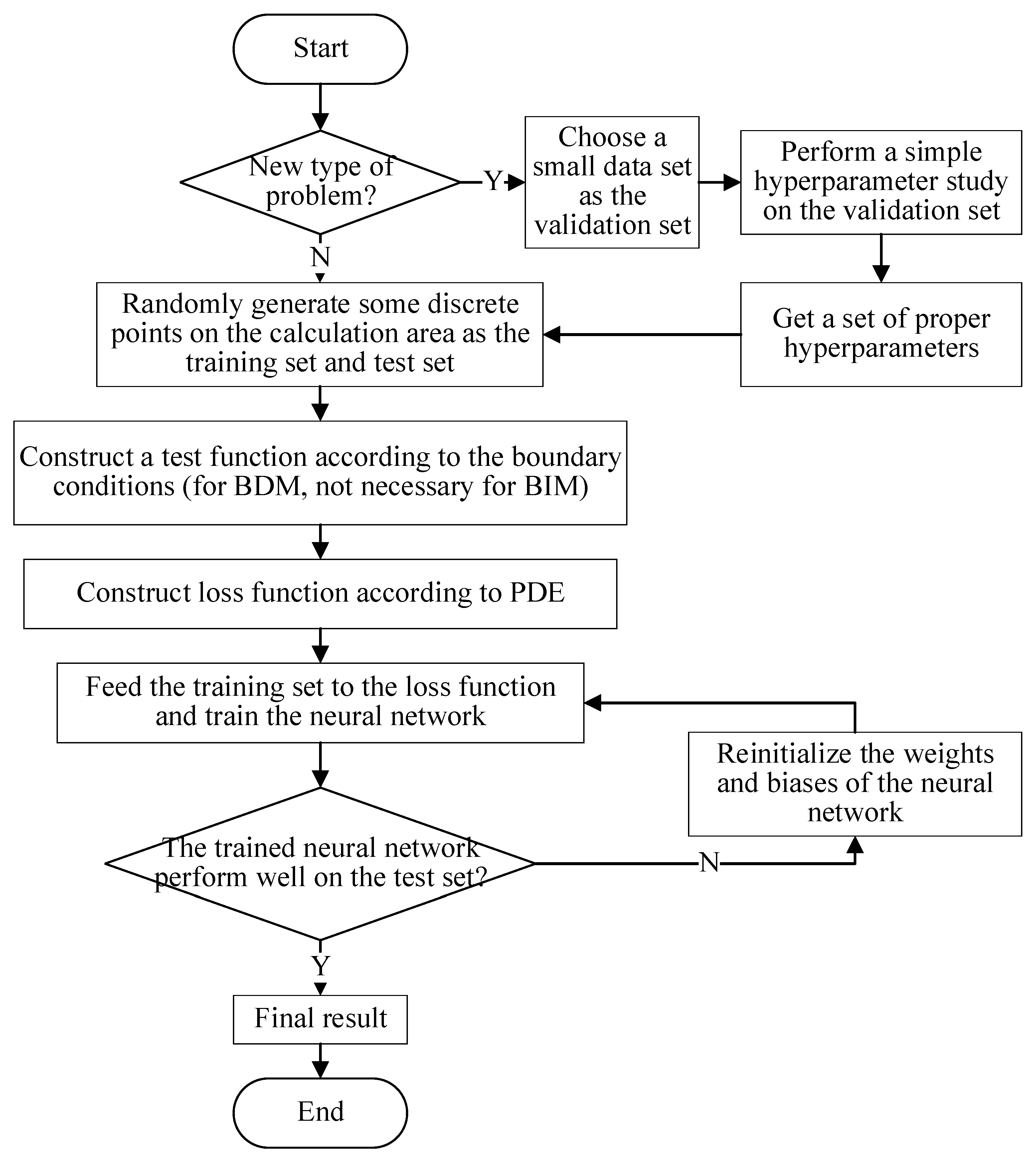
Figure 1 shows the flowchart of PIDL method, which can be descripts as follows. Before solving the neutron diffusion problem, it’s needed to classify the type of problem. For example, whether the problem is two-dimensional or three-dimensional, transient or steady, a single-zone problem or a multi-zone problem, and so on. When solving the new type of problem, a small data set should be chosen as the validation set, which is used to perform a simple and fast hyperparameter research to determine an appropriate set of hyperparameters. Then, the training set and test set are built by randomly generating the discrete points on the calculation domain. The construction of trial function is necessary for BDM, but is unnecessary for BIM, while the constructions of loss functions based on the PDE are both necessary. After being trained on training set, neural network is evaluated on the test set. If its performance is not satisfactory enough, the weights and biases of the network will be reinitialized for retraining. Otherwise, the final result will be given.
It should be noted that, in most cases, the hyperparameters search is only required for different types of problems rather than every problem, i.e., the similar problems can usually be solved using the similar hyperparameters. When considering a new type of problem, only a small validation set is needed to determine the proper set of hyperparameters, which is recommended to solve other similar problems.
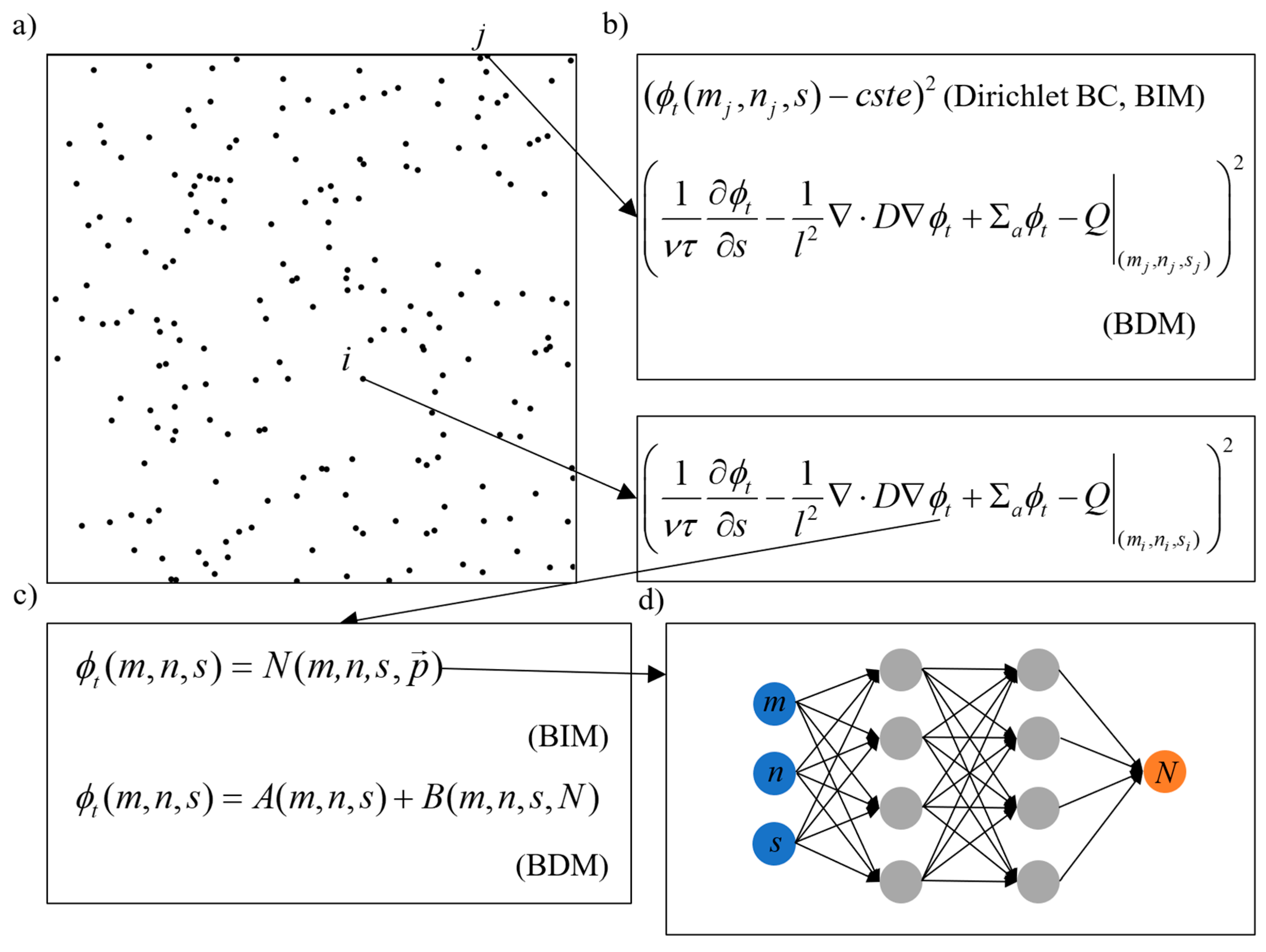
The PIDL method does not require any output data (for the diffusion equation, the output data is the point-wise neutron flux value), but employ the physical model provided by the diffusion equation itself as the calculation guidance. The underlining idea of PIDL is implemented as follows. It first assumes a trial function ϕt containing undetermined parameters to be the solution of the PDE (in our case, it is the diffusion equation), and then it tests whether the trial function can fit the PDE at certain arbitrary picked discrete points. A gradient based descent method is followed to adjust the undetermined parameters to improve the global fitting performance until the satisfactory solution is achieved. Figure 2 shows the schematic flowchart of the PIDL method. The implementation difference existed in BDM and BIM (which are two different PIDL realization in this work) are also briefly illustrated in Figure 2, and these differences will be elaborated soon.
As shown in Figure 2a, several discrete points are randomly selected in the computation domain. The internal points, such as point i, are necessary for both BDM and BIM. The boundary points, such as point j, are only necessary for BIM. At each point, a local loss function is established to measure the fitting performance. As shown in Figure 2b, the local loss function at internal point i is always defined by the square of the value of PDE at this point for either BDM or BIM. The local loss function at boundary point j changes in BIM, since it is employed to measure whether the trial function can fit the BC well. The top formula in Figure 2b presents an example of local loss function on the boundary for the constant Dirichlet BC. However, in actual calculation, it is almost impossible for the trial function to perfectly match BCs. This mismatch may interfere with the calculation of internal points and negatively affect the calculation accuracy of final results. Fortunately, the problem of BCs fitting does not exist in BDM, since the constructed trial function in BDM naturally fit the BCs perfectly. The global loss function on the train set, namely the optimization object, is then defined upon the local loss functions as:
where Ntrain is the total number of discrete points in the training set; represent the local loss function at a certain point k. In a similar manner, is defined as the global loss function on the test set.
In addition to the BC treatments, there are two important questions need to be addressed by the PIDL: the optimization strategy for the global loss function, and the adjustment of the trial function. These questions are very difficult to answer two decades ago, but now with the help of artificial intelligence toolbox such as TensorFlow, the difficulties of these questions are significantly mitigated and both questions can be solved by a simple subroutine within the toolbox. In this work, the automatic differentiation technique and the quasi-Newton based optimization method, namely Limit memory BFGS (L-BFGS) method [34], are applied to address these two questions. The L-BFGS technique is one of the most commonly used quasi-Newton method for solving unconstrained nonlinear optimization problems. In comparing to other optimization method, the L-BFGS method shows higher convergence rate and lower memory requirement. The automatic differentiation and L-BFGS method can be realized by calling built-in functions in TensorFlow. Both of these capabilities are enabled by directly calling built-in functions in TensorFlow. A parameter known as ftol varies with different applications when calling these build-in functions. It is a criterion by which L-BFGS stops the iteration. A larger ftol means stopping iteration earlier and deviating more from the extreme.
The equations in Figure 2c presents the basic idea of trial function construction. For BIM, it is defined as:
where is an ANN function with representing all undetermined parameters in N, including weights and biases. For BDM, the trial function is defined as:
where A(m, n, s) is the function that fits the BCs and B(m, n, s, N) is the function that has no contribution to the BCs. Taking the constant Dirichlet BC as an example, A should be equal to the value required by BC on this boundary and B should be zero on this boundary. Obviously, the specific expressions of A and B depends entirely on BCs, which is one of the trickiest problems in BDM. An innovative approach to obtain the expressions of A and B for some special BCs for BDM is elaborated in Section 2.3.
2.3. Trial Functions for Special BCs in BDM
A construction of trial function for special BCs means to give a concrete form of A(m, n, s) and B(m, n, s, N) in the BDM implementation. The construction should have two apparent features. The first is that the construction for certain BCs should not be unique, since the trial function fitting the BCs is not unique. Therefore, the trial function constructed by BDM corresponding to certain BCs in this work is not the only possible solution. The second is that the construction should only depend on the BCs, not the governing equations. Thus, different governing equations with same BCs may share common constructions. Furthermore, the construction should not be affected by the parameters changing of the governing equations within the computation domain. In this section, eight constructions of trial functions for four kind of BCs in both transient and steady state conditions are outlined by following the boundary treatment ideas proposed by [33].
For time-dependent conditions, in addition to the spatial BCs, an initial condition (IC) is required, which can be assumed as:
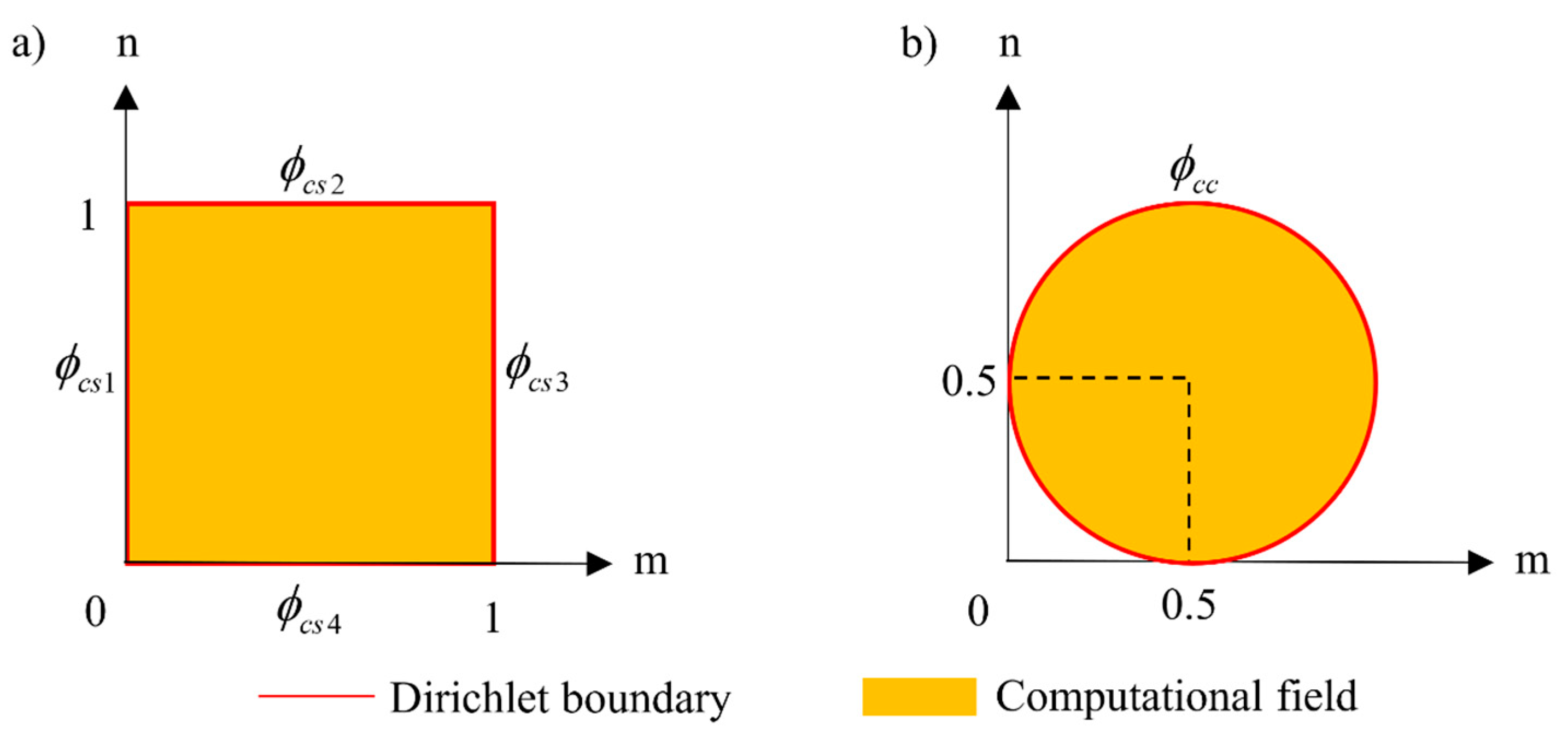
In this paper, two typical geometries shown in Figure 3 will be used to illustrate the setting of trial function construction for spatial BCs.
The Dirichlet BC (such as zero-flux boundary) is commonly used in reactor physics. In Figure 3, the neutron flux on the physical boundaries is set as , which is only defined on the boundary and can be described in Equations (9) and (10) for square boundary (SB) and circular boundary (CB), respectively.
Inspired by a treatment for a time-independent problem [33], a possible form of trial function is proposed to fit Equations (8) and (9), in which the functions a(m, n, s) and a0(m, n) are introduced to form this trial function. They can be described as:
where
Due to the continuity of the neutron flux function, the continuity of the IC in Equation (8) and the spatial BCs in Equation (9) is admitted, which can be described as:
With Equation (13), some properties of a and a0 can be obtained as:
Substituting Equation (14) into Equation (11), it is evident that the trial function formed by Equation (11) fits Equations (8) and (9).
Similarly, a possible form of trial function fitting Equations (8) and (10) can be described as:
where . The definition domain of ϕcc is a circuit, and A needs to be defined in the entire calculation domain. Therefore, ϕcc should be extended to the entire calculation domain. Sometimes, A obtained by directly extending ϕcc may be discontinuous at the center of the circuit, thus in this case, the discrete point at the center should be avoided.
For the steady-state problem, Equation (11) can be simplified to [33]:
and Equation (15) can be simplified to:
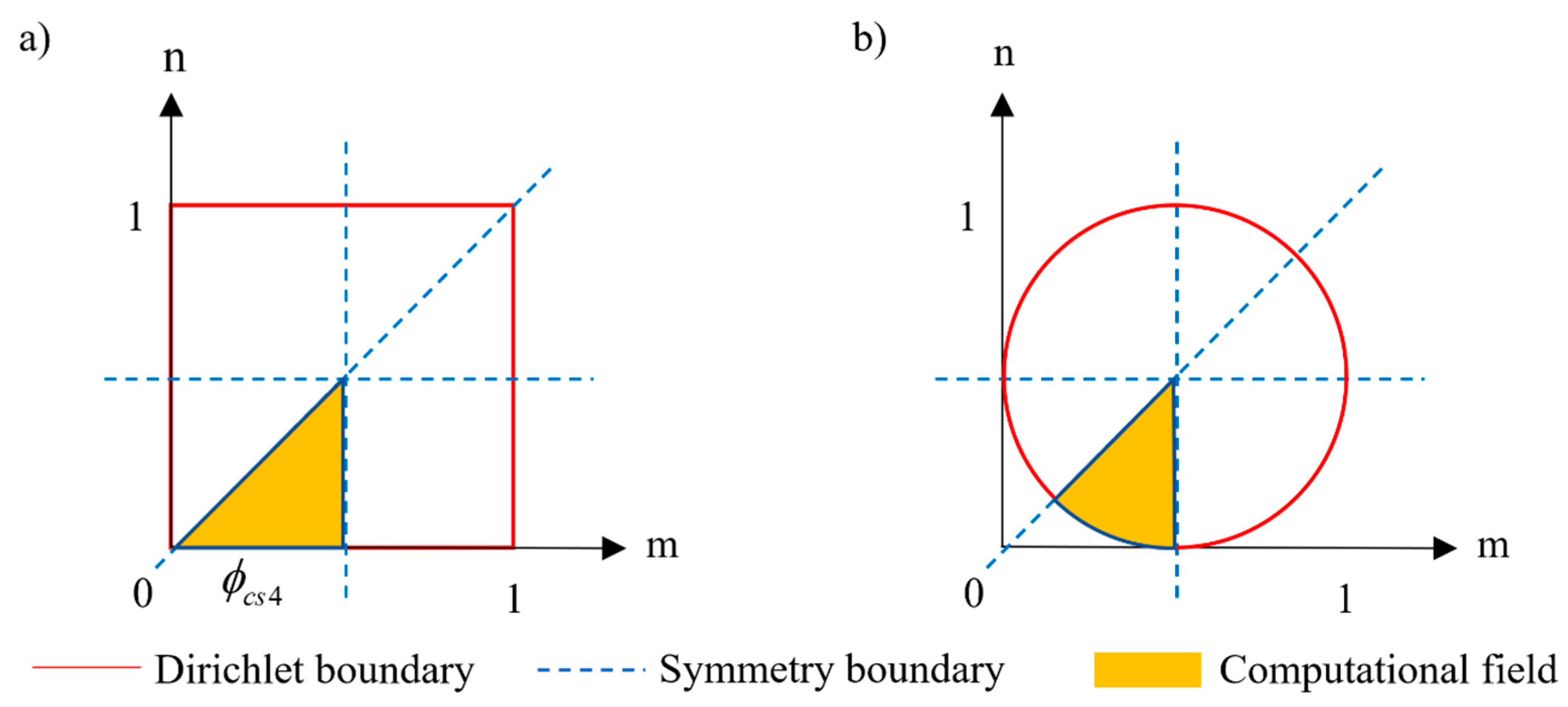
In addition to the Dirichlet BC, the Neumann BC, such as the symmetry boundary, is sometimes used in reactor physics calculations to reduce the computational cost by applying the symmetry characteristics. As shown in Figure 4, a yellow domain with one Dirichlet boundary (physical boundary) and two Neumann boundaries (symmetry boundary) can be used to substitute the whole domain in the calculation.
The left and right Neumann BCs and the Dirichlet BC shown in Figure 3 can be respectively described as follows:
A similar but more simplified trial function is proposed to fit Equations (8), (18) and (19), in which and are introduced to form this trial function. They are described as:
where
Due to the continuity of the neutron flux function, the continuity of the IC in Equation (8) and the spatial BCs in Equation (9) are admitted, which can be described as:
Substituting Equations (14) and (23) into Equation (21), it is evident that the trial function formed by Equation (21) fits Equations (8), (18) and (19).
Similarly, a possible form of trial function fitting Equations (8), (18) and (20) can be described as:
Similar to Equation (15), should be extended to the entire calculation domain and the discrete point at the center should be avoided. The proof for this trial function is presented in Appendix A.
For the steady-state problem, Equation (21) can be simplified to:
and Equation (24) can be simplified to:
3. Results and Discussion
In this section, some numerical problems based on the neutron diffusion equation are employed to examine the computational performance of the BDM and BIM. Four cases are used to evaluate different performance aspects of the methods. Case 1 compares the accuracy and efficiency of BDM and BIM. Case 2 assesses the choice of the activation function type in DL neural network. The activation function is an important element in the DL method used to determine the hidden unit of the network. Case 3 investigates the influences of some important hyperparameters used in BDM on the calculation results. Finally, Case 4 demonstrates the potential of BDM to handle more complicated geometry case.
3.1. Case 1—Comparison of BDM and BIM
As mentioned in Section 2.2, BIM introduces some extra points on the boundary to ensure the trial functions fit the BCs as much as possible, while BDM constructs the trial functions to perfectly fit the BCs. As a result, one obvious advantage of BDM over BIM is that there is no error caused by the BCs in BDM. However, the method to construct the trial functions in BDM is more complex than that of BIM as shown in Section 2.3, which may result in higher computational costs. Therefore, Case 1 is set up to gain a better understanding of the calculation efficiency and accuracy of these two methods.
Case 1 is a two-dimensional time-dependent mono-energetic neutron diffusion problem with homogeneous media and zero-flux boundaries in the Cartesian geometry, as shown in Figure 3a. The governing equation of the problem is shown as Equation (3). The external source is prescribed as:
and the initial condition is given as:
The values of all parameters used in Case 1 are summarized in Table 1.
The analytical solution of this problem is expressed as follows:
which is used as the exact reference solution for the BIM and BDM solutions.
In the calculations of Case 1, 1000 random data points within the computing phase space are chosen as the training set to train the neural network. Specifically, 100 random data points on phase space boundaries are used in BIM. The test set used to assess the accuracy of ANN consists of 8000 data points with the same distribution range as the training set. For Case 1, the feed-forward neural network is constructed with two hidden layers and 20 neurons per hidden layer. A hyperbolic tangent function is used as the activation function in the network. The parameter ftol is set as 10−7 for both two methods. The average predicted error (APE) defined in Equation (30) is used to evaluate the accuracy of the DL neural network
where Ntest is the number of data points in the test set, ϕp is the trial function trained by the DL neural network, and ϕa is the analytical solution as Equation (29). The training time is used to evaluate the computational efficiency.
At present, there is no theory that can exactly give the optimal initial value of the weight and bias in the neural network. The usual practice is to randomly assign them values within a certain range. However, when applying the gradient descent method to optimize the neural network, the selection of the initial point will have a great impact on the optimization speed and results. In order to minimize the error caused by the randomness of the initial values of the weights and biases, 25 different initial values are used to calculate and count the average results in Case 1.
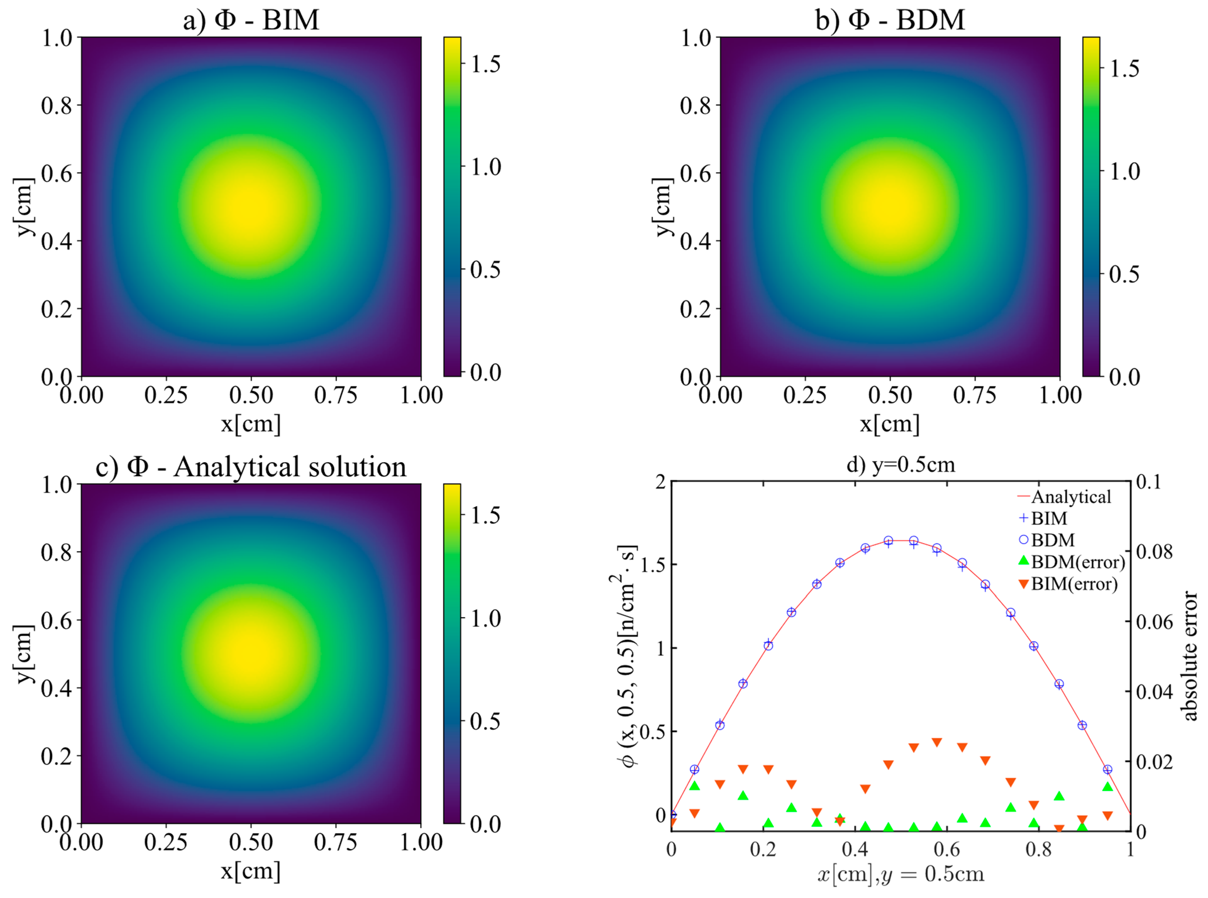
The calculation results of PIDL method with BDM and BIM trial solutions at t = 0.5 s are shown in Figure 5, which indicates that both BDM and BIM can get a good agreement with the analytical solution for this case. Figure 5d also shows the distribution of absolute errors. The error of BDM is generally lower than BIM. The maximum error of BDM is 1.87 × 10⁻⁴, and the average absolute error is 5.95 × 10⁻⁴, while the maximum and averaged errors of BIM are 1.27 × 10⁻² and 5.41 × 10⁻², respectively.
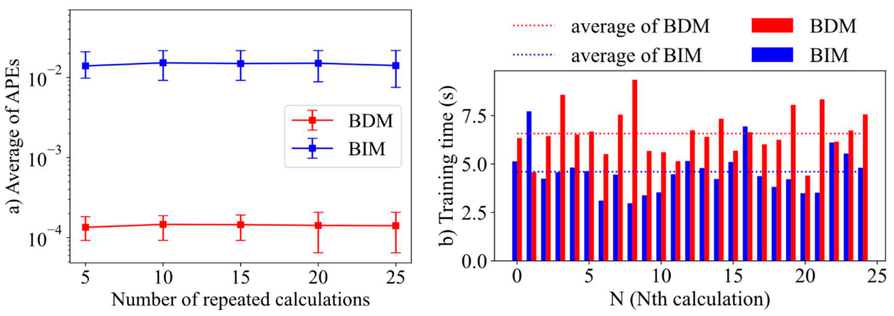
The accuracy and efficiency of BDM and BIM for Case 1 are further compared in Figure 6, including the time-averaged APEs and the training time. As shown in Figure 6a, the time-averaged APEs of BDM and BIM with different repeat times both vary within a narrow scope, which indicates that the PIDL method is stable for neutron diffusion solving. Figure 6a also shows that the APEs of BDM are nearly two orders of magnitude smaller than that of BIM, indicating that the accuracy of BDM is far higher than that of BIM. Figure 6b shows the training time of the PIDL neural network with BDM and BIM, their comparisons demonstrate that the BDM usually takes more training time than BIM, since the form of trial function of BDM is usually more complex than that of BIM. The average training time of BDM is about 1.97 s longer than that of BIM. As a result, no boundary error is introduced during the training of BDM, but its training time will be extended.
In summary, the results of Case 1 indicate that the BDM usually shows higher accuracy than BIM, which can offset the disadvantage caused by lower calculation efficiency. Since the training time for both methods are essentially in the same scale, this work herein adopts only the BDM for the subsequent case problems.
3.2. Case 2—Choice of Activation Function
An important aspect in DL method is choosing the type of hidden unit in the network. Activation function is used for this purpose. Even though the design of hidden unit is a hot topic in DL, there is yet no dominant principle to choose the activation function. As for now, two common activation functions were used in PIDL of this study: the logistic sigmoid (sigmoid for short) and the hyperbolic tangent function (tanh for short). The expressions of these two activation functions are given below:
Both the tanh and sigmoid activation functions are considered in the Case 2 test problem to assess their performance for neutron diffusion problems. Some other popular activation functions, such as ReLU and leaky ReLU, are not used in this work. Since both of these two activation functions are linear, and their second-order gradients are equal to 0, which leads to the premature termination of optimization process for neutron diffusion problems.
Case 2 has the same problem configuration at Case 1, but only works on part of Case 1 domain by utilizing its symmetric property with both Dirichlet and Neumann BCs enforced as shown in Figure 4a. Besides, other parameters including the structure of neural network, and the value used in Case 2 remain identical to that of Case 1. The size of training set of BDM and BIM is 1000, and the size of test set is 8000.
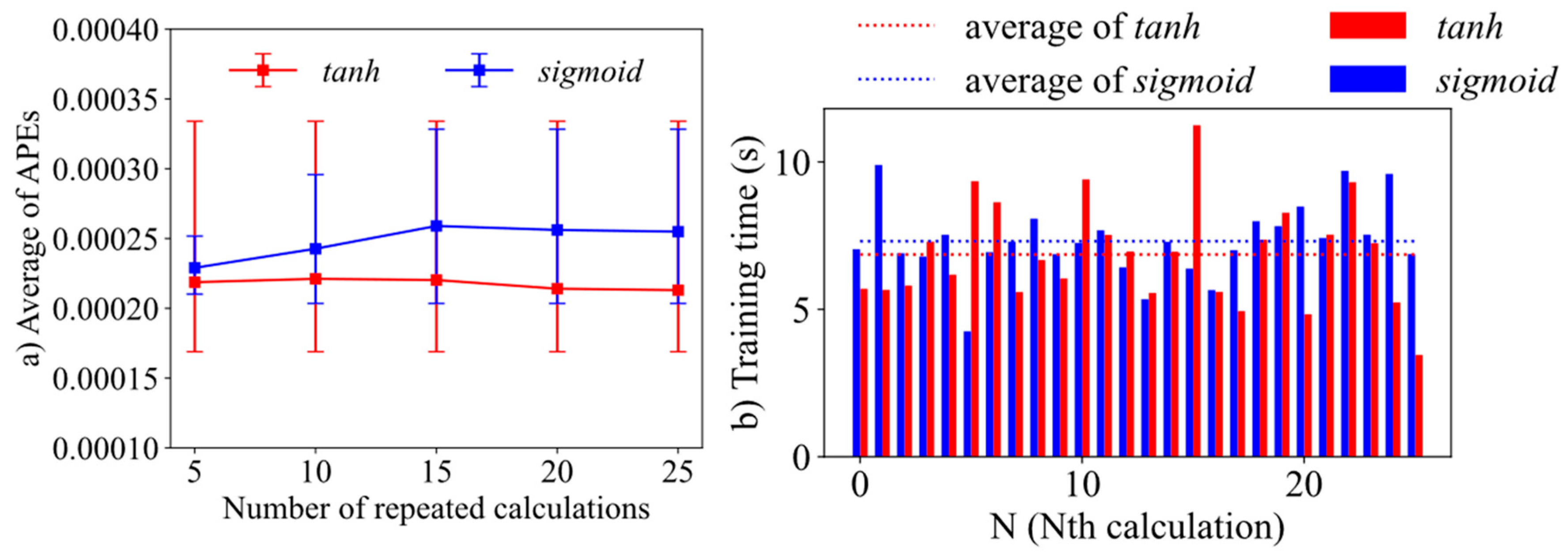
The results of the comparison of calculation accuracy and efficiency when using tanh or sigmoid as activation function in Case 2 are illustrated in Figure 7. As shown in Figure 7a, the average value of APE using tanh activation function within 25 repeated calculations is smaller than that with sigmoid activation function, which indicates a higher accuracy of using tanh as the activation function. In Figure 7b, the training time for each calculation corresponding to tanh and sigmoid activation function is compared, in which the average training time with tanh activation function is shorter than that with sigmoid.
In summary, this case indicates that the tanh activation function shows better performance than that of sigmoid. Therefore, tanh is used herein as the activation function for the rest of test problem calculations.
3.3. Case 3—Impact of Hyperparameters
Similar to the other DL methods, there are many important hyperparameters in the PIDL with BDM. It is noteworthy to investigate the sensitivities of hyperparameters to the method. In this work, the following two hyperparameters are selected for this purpose: the number of hidden layers Nl and the number of neutrons in each hidden layer Nn. In Cases 1 and 2, Nl = 2 and Nn = 20 were used to construct the network, but they may not be the optimum ones. The Case 3 test problem discussed in this subsection is designed to investigate the impact of these hyperparameters to the BDM method. The size of training set is 5000, and the size of test set is 10,000.
This problem is a steady-state two-dimensional mono-energetic neutron diffusion problem with heterogeneous media as shown in Figure 2a. The external source term is prescribed as
The zero-flux boundaries are applied to each side of the domain, and the values of problem parameters used in Case 3 are summarized in Table 2. The reference value of Case 3 is provided by the multi-physics software COMSOL [35], which used FEM to provide higher order numerical solutions to PDE problems.
In the application of PIDL, an important question is whether the performance of the neural network on test set after training can meet the expected requirements. The quantity losstest is used as a metric to evaluate whether the trained neural network is successful. In this work, the neural network with losstest greater than 10−2 is considered as a failure training. For each neural network with a set of hyperparameters, 10 successful trainings are expected for analysis, i.e., for each proposed neural network, many times repeatedly training should be taken until 10 successfully trained neural networks are obtained. In general, 10 successfully trained ANNs can be obtained. But in a few cases, it’s extremely difficult or impossible to achieve 10 successfully trained neural networks. Therefore, in this work, an upper limit of failed training Nfail = 50 is set to reduce meaningless calculations. In all calculations in the Case 3, Nfail cannot be greater than 50 for each attempt to successful training. If under a certain set of hyperparameters, Nfail reaches 50, it simply indicates this network structure is be suitable for the calculation of Case 3.
The impact of two hyperparameters (Nl and Nn) on APE, training time and success rate of neural network training are summarized in Figure 8, Figure 9 and Figure 10, respectively. It should be noted that more than 50 networks with the structure Nl = 1 and Nn = 5 have been tried to train. But all these networks have failed. Therefore, this structure is not included in Figure 8 and Figure 9. One possible explanation for the failure of this network structure is that this structure is too simple to be adequate for the calculation in Case 3. Additionally, for most cases, failed training has much less training time than successful training, but this is meaningless since the failed training fell into a local minimum shortly after the start. In this case, the APEs of the failed training networks are often higher than that of the successfully trained networks.
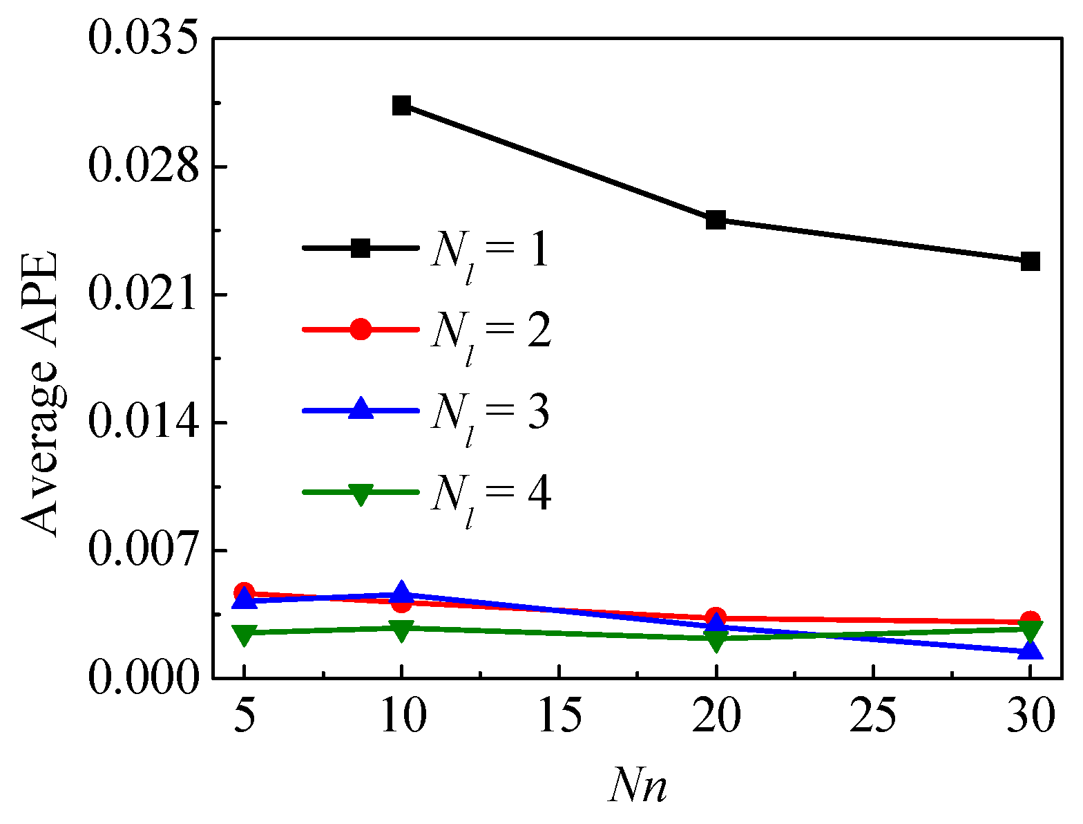
Figure 8 shows the average APE varying with Nl and Nn. The general trend is that increasing Nn can reduce the APE. But for a few structures, such as Nl = 4 and Nn > 20, the increase of Nn will cause the increase of APE. Increasing Nl from 1 to 2 greatly reduces the APE. But when Nl continues to increase, the decrease in APE decreases sharply, even when Nn = 30, APE does not decrease but increase. This phenomenon may be caused by the large ftol that stoping the optimization in advance, thus the fitting ability of the complex neural network is not fully exerted. Besides, as neural network become more complex, the problem of overfitting becomes more and more serious. A complex neural network can perform well on the training set, but it does not always perform well on the test set.
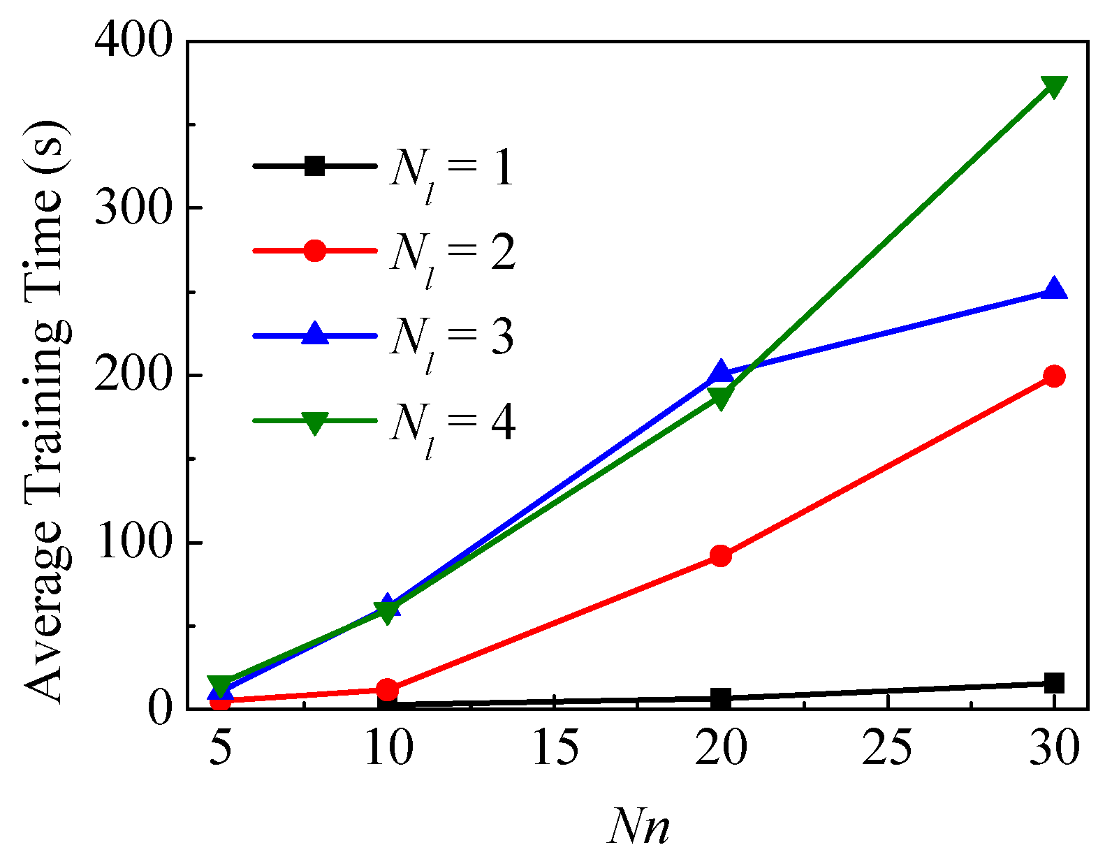
Figure 9 shows the averaged training time varying with Nl and Nn, in which the larger Nl and Nn lead to longer training time. Considering the effect of fluctuations in the computer’s running conditions in training time, it is acceptable to have some cases that do not conform to the above rule.
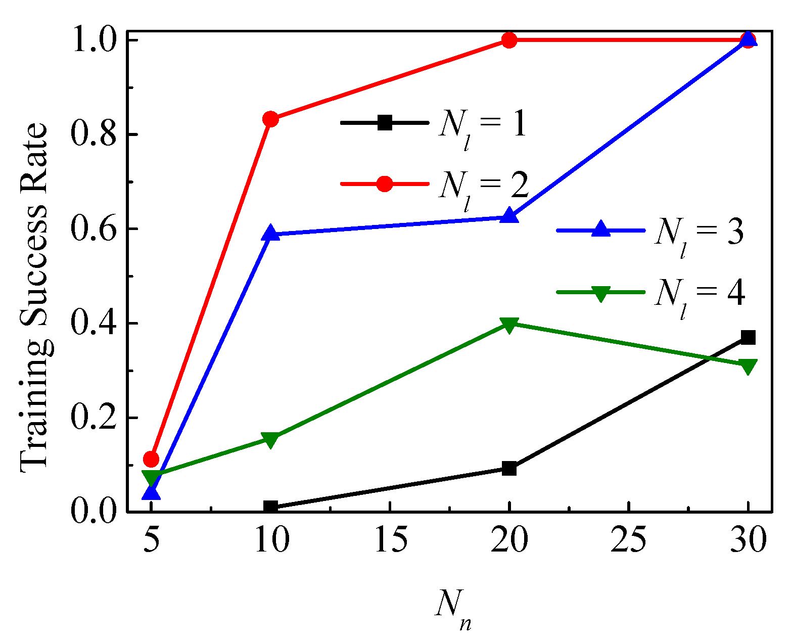
Figure 10 gives the training success rate varying with Nl and Nn, which shows a different regulation from APE and training time. The success rate of training in the Figure 10 is slightly lower than the actual success rate, because every attempt ends with a successful training. But the statistical results under 10 attempts are sufficient for qualitative analysis. The success rate of training is not simply increasing with the complexity of the neural network. For some simple neural networks (Nl = 2, Nn = 5 and Nl = 1, Nn = 10), the success rate is very low but not zero, which means that these two neural networks have sufficient fitting ability to meet the restriction of losstest. The low success rate may be explained by the fact that most of the local extreme points of these two neural networks can’t meet this restriction. For some complex neural networks (Nl = 4), the success rate doesn’t exceed 50%, which is worse than a simpler neural network (Nl = 2). For a neural network with a complexity between simple and complex, there is almost no specific rule for the success rate. In the actual application of DL, the optimal choice of neural network structure is often different for different issues. The optimal choice of neural network structure is often based on experience rather than theory. In general, we should avoid choosing a too simple or too complex neural network. Only after determining the issue and the training set, can we choose a better network structure.
In conclusion, for a particular issue, it is recommended to first determine the size of the training set, which relies on the independent variables number in the issue, and the degree of the physical parameters change in the calculation domain. In the choice of network structure, overly simple networks should be absolutely avoided. Although an overly complex ANN may have better performance in term of calculation accuracy, considering its low success rate of training and long training time, it’s recommended to choose an overly complicated ANN carefully.
3.4. Case 4—Application in Complex Geometry
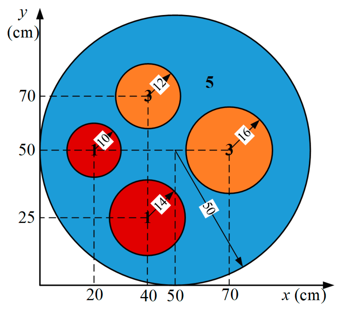
The last test problem [36], namely Case 4, is calculated to demonstrate the BDM in solving the problems with complex geometry. Case 4 is a steady-state diffusion problem governed by Equation (4), in which = 100 cm. The geometric conditions of Case 4 are shown in Figure 11. The space domain of the problem is divided into five regions with three materials indicated as Area 1, Area 3 and Area 5, respectively, whose physical properties are given in Table 3. The zero-flux boundaries, as shown in Figure 3b, are imposed for the problem. The selected neural network in BDM is a feed-forward network with four hidden layers and 40 neutrons per hidden layer (i.e., Nl = 4 and Nn = 40), and a hyperbolic tangent activation function. The network is trained under the condition of ftol = 2.2 × 10⁻¹⁶. The size of training set is 10,000 and no test set is set in this case.
The result calculated by COMSOL is used as the reference solution for comparison with the BDM results. The COMSOL is calculated with 1097 nodes and 2104 elements, and the grid independent is verified. The tolerance is set as 0.001. Figure 12a,b shows the comparison of BDM solutions and COMSOL solutions. For clarity, Figure 12c,d give the neutron distributions along two characteristic lines with y = 50 cm and x = 40 cm, in which the BDM solutions agree well with those of COMSOL, indicating that the proposed BDM can simulate the neutron diffusion processes with high accuracy and flexibility.
To further analyze the accuracy of proposed BDM, the PDE residual is defined as:
where φ* is the numerical result. This value is used to exam the precision of the numerical solutions.
Over the calculation domain, the maximum and averaged PDE residuals of BDM are 5.9 × 10⁻² and 3.4 × 10⁻³, respectively, while these of COMSOL are 6.4 × 10⁻² and 9.5 × 10⁻³, respectively. The PDE residual of BDM and COMSOL along y = 50 cm and x = 40 cm are shown in Figure 12e,f, which show that the BDM has higher accuracy than COMSOL.
4. Conclusions
The demands of advance reactor simulations, such as multi-physics modeling and complicated geometries, put forward higher requirements for the traditional mesh-based methods. To overcome these difficulties, this paper introduces two mesh-free physics-informed deep learning (PIDL) method, including the boundary dependent method (BDM) and the boundary independent method (BIM), which give a continuous and symbolic solution, and proposes some novel construction of trial function. By perfectly fitting the BCs, the BDM can be regarded as the recommended PIDL method based on its higher performance. The influence of some important hyper-parameters, such as activation function and network structure, is discussed in a more complicated test problem to improve the performance of BDM. The succussed of BDM in a complex geometry test problem shows that the BDM has great potential in sophisticated problems.
Some novel treatments on BCs for BDM are presented in this work. Although the calculation efficiency of BDM is lower than that of BIM, the obvious advantage of BDM in accuracy still makes BDM a better choice. Among two common activation functions, tanh is proposed to be used in artificial neural networks because of its higher accuracy and efficiency. And in practical application of BDM, the determination of training set size based on the dimension of the problem and the number of zones is proposed. During the calculation, it’s recommended to try to choose a larger training set to ensure that the calculation results will not deviate too much from the true solution, and find a good network structure according to the size of training set. Both too simple and too complicated network structure should be avoided. The simulation results show that the BDM can handle complicated geometry and multi-region problems with higher accuracy and flexibility. This paper could provide some new ideas for solving multi-physics and complicated geometry problems in neutron diffusion calculations.
For future work, we will extend the BDM to solve k-eigenvalue problem, neutron transport problem and multi-physics coupling problem. Besides, the improvement of BDM for the multi-region problem and the error prediction in BDM will also be analyzed in our future works.
Author Contributions
Conceptualization, Y.M.; methodology, Y.X., Y.W., Y.M. and Z.W.; software, Y.X. and Y.M.; validation, Y.X., Y.M. and Y.W.; formal analysis, Y.M. and Z.W.; investigation, Y.W.; resources, Y.M. and Z.W.; data curation, Y.X.; writing—original draft preparation, Y.X. and Y.M.; writing—review and editing, Z.W. and Y.W.; visualization, Y.X. and Y.W.; supervision, Y.M. and Z.W.; project administration, Y.M.; funding acquisition, Y.M. All authors have read and agreed to the published version of the manuscript.
Funding
This research was funded by National Natural Science Foundation of China (Grant No. 11875330), and the NSAF (Grant No. U1830118).
Conflicts of Interest
The authors declare no conflict of interest.
Appendix A
In this section, a proof of the trial function formed by Equation (24) in Section 2.3 will be made. The goal of the proof is to prove that this trial function can fit Equations (8), (18) and (20) well.
The proof of fitting Equation (8) is very simple. Let s = 0, Equation (24) becomes:
From this relationship we have . We define a assemble of points on a unit circle as:
Let , Equation (24) becomes;
Due to the continuity of the neutron flux function, the continuity of the initial condition in Equation (8) and the spatial boundary condition in Equation (20) is admitted, which can be described as:
From this relationship we have .
The proof of fitting Equation (18) is based on a conversion from Cartesian coordinates to Polar coordinates. The angle θ is defined as
With this definition, we have the coordinate conversion . We consider an extended function that is defined in the whole calculation domain. It is evident that . Thus, we have:
With Equation (A5), we have:
Equation (A6) thus becomes:
Due to the continuity of the neutron flux function, the continuity of the spatial boundary condition in Equations (18) and (20) is admitted, which can be described as
When , we have , and Equation (A8) becomes:
Thus, we have:
When , we have:
With Equations (A8) and (A11), we have:
Combining Equations (A12) and (A13), the fitting of Equation (18) is proved.
References
- Bell, G.I.; Glasstone, S. Nuclear Reactor Theory; US Atomic Energy Commission: Washington, DC, USA, 1970.
- Duderstadt, J.J. Nuclear Reactor Analysis; Wiley: Hoboken, NJ, USA, 1976. [Google Scholar]
- Kang, C.M.; Hansen, K. Finite element methods for reactor analysis. Nucl. Sci. Eng. 1973, 51, 456–495. [Google Scholar] [CrossRef]
- Varga, R.S. Numerical solution of the two-group diffusion equations in xy geometry. IRE Trans. Nucl. Sci. 1957, 4, 52–62. [Google Scholar] [CrossRef]
- Vondy, D.; Fowler, T.; Cunningham, G. VENTURE: A Code Block for Solving Multigroup Neutronics Problems Applying the Finite-Difference Diffusion-Theory Approximation to Neutron Transport; Oak Ridge National Lab.: Oak Ridge, TN, USA, 1975. [Google Scholar]
- Dodson, Z.; Kochunas, B.; Larsen, E. The Stability of Linear Diffusion Acceleration Relative to CMFD. J. Nucl. Eng. 2021, 2, 336–344. [Google Scholar] [CrossRef]
- Berg, J.; Nyström, K. A unified deep artificial neural network approach to partial differential equations in complex geometries. Neurocomputing 2018, 317, 28–41. [Google Scholar] [CrossRef] [Green Version]
- Bao, H.; Dinh, N.; Lin, L.; Youngblood, R.; Lane, J.; Zhang, H. Using deep learning to explore local physical similarity for global-scale bridging in thermal-hydraulic simulation. Ann. Nucl. Energy 2020, 147, 107684. [Google Scholar] [CrossRef]
- Elhareef, M.H.; Wu, Z.; Ma, Y. Physics-informed deep learning neural network solution to the neutron diffusion model. In Proceedings of the the International Conference on Mathematics and Computation Methods Applied to Nuclear Science and Engineering (M&C 2021), Raleigh, NC, USA, 3–7 October 2021. [Google Scholar]
- Kim, T.K.; Park, J.K.; Lee, B.H.; Seong, S.H. Deep-learning-based alarm system for accident diagnosis and reactor state classification with probability value. Ann. Nucl. Energy 2019, 133, 723–731. [Google Scholar] [CrossRef]
- LeCun, Y.; Bengio, Y.; Hinton, G. Deep learning. Nature 2015, 521, 436–444. [Google Scholar] [CrossRef] [PubMed]
- Qin, S.; Zhang, Q.; Zhang, J.; Liang, L.; Zhao, Q.; Wu, H.; Cao, L. Application of deep neural network for generating resonance self-shielded cross-section. Ann. Nucl. Energy 2020, 149, 107785. [Google Scholar] [CrossRef]
- Collobert, R.; Weston, J.; Bottou, L.; Karlen, M.; Kavukcuoglu, K.; Kuksa, P. Natural language processing (almost) from scratch. J. Mach. Learn. Res. 2011, 12, 2493–2537. [Google Scholar]
- Hermann, K.M.; Kocisky, T.; Grefenstette, E.; Espeholt, L.; Kay, W.; Suleyman, M.; Blunsom, P. Teaching machines to read and comprehend. Adv. Neural Inf. Process. Syst. 2015, 28, 1693–1701. [Google Scholar]
- Jean, S.; Cho, K.; Memisevic, R.; Bengio, Y. On using very large target vocabulary for neural machine translation. arXiv 2014, arXiv:1412.2007. [Google Scholar]
- Wang, W.; Song, W.; Chen, C.; Zhang, Z.; Xin, Y. I-vector features and deep neural network modeling for language recognition. Procedia Comput. Sci. 2019, 147, 36–43. [Google Scholar] [CrossRef]
- Krizhevsky, A.; Sutskever, I.; Hinton, G.E. Imagenet classification with deep convolutional neural networks. Adv. Neural Inf. Process. Syst. 2012, 25, 1097–1105. [Google Scholar] [CrossRef]
- Li, Y.; Zhang, D.; Lee, D.-J. IIRNet: A lightweight deep neural network using intensely inverted residuals for image recognition. Image Vis. Comput. 2019, 92, 103819. [Google Scholar] [CrossRef]
- Tompson, J.J.; Jain, A.; LeCun, Y.; Bregler, C. Joint training of a convolutional network and a graphical model for human pose estimation. Adv. Neural Inf. Process. Syst. 2014, 27, 1799–1807. [Google Scholar]
- Hinton, G.; Deng, L.; Yu, D.; Dahl, G.E.; Mohamed, A.-r.; Jaitly, N.; Senior, A.; Vanhoucke, V.; Nguyen, P.; Sainath, T.N. Deep neural networks for acoustic modeling in speech recognition: The shared views of four research groups. IEEE Signal Process. Mag. 2012, 29, 82–97. [Google Scholar] [CrossRef]
- Sainath, T.N.; Kingsbury, B.; Mohamed, A.-r.; Dahl, G.E.; Saon, G.; Soltau, H.; Beran, T.; Aravkin, A.Y.; Ramabhadran, B. Improvements to deep convolutional neural networks for LVCSR. In Proceedings of the 2013 IEEE Workshop on Automatic Speech Recognition and Understanding, Olomouc, Czech Republic, 8–12 December 2013; pp. 315–320. [Google Scholar]
- Fujii, M.; Takahashi, A.; Takahashi, M. Asymptotic expansion as prior knowledge in deep learning method for high dimensional BSDEs. Asia-Pac. Financ. Mark. 2019, 26, 391–408. [Google Scholar] [CrossRef] [Green Version]
- Galib, S.M. Applications of Machine Learning in Nuclear Imaging and Radiation Detection; Missouri University of Science and Technology: Rolla, MO, USA, 2019. [Google Scholar]
- Galib, S.; Bhowmik, P.; Avachat, A.; Lee, H. A comparative study of machine learning methods for automated identification of radioisotopes using NaI gamma-ray spectra. Nucl. Eng. Technol. 2021, 53, 4072–4079. [Google Scholar] [CrossRef]
- Sasaki, M.; Sanada, Y.; Katengeza, E.W.; Yamamoto, A. New method for visualizing the dose rate distribution around the Fukushima Daiichi Nuclear Power Plant using artificial neural networks. Sci. Rep. 2021, 11, 1857. [Google Scholar] [CrossRef] [PubMed]
- Han, J.; Jentzen, A.; Weinan, E. Solving high-dimensional partial differential equations using deep learning. Proc. Natl. Acad. Sci. USA 2018, 115, 8505–8510. [Google Scholar] [CrossRef] [Green Version]
- Raissi, M.; Perdikaris, P.; Karniadakis, G.E. Physics-informed neural networks: A deep learning framework for solving forward and inverse problems involving nonlinear partial differential equations. J. Comput. Phys. 2019, 378, 686–707. [Google Scholar] [CrossRef]
- Sirignano, J.; Spiliopoulos, K. DGM: A deep learning algorithm for solving partial differential equations. J. Comput. Phys. 2018, 375, 1339–1364. [Google Scholar] [CrossRef] [Green Version]
- Abadi, M. TensorFlow: Learning functions at scale. In Proceedings of the 21st ACM SIGPLAN International Conference on Functional Programming, Nara, Japan, 18–24 September 2016; p. 1. [Google Scholar]
- Abadi, M.; Barham, P.; Chen, J.; Chen, Z.; Davis, A.; Dean, J.; Devin, M.; Ghemawat, S.; Irving, G.; Isard, M. Tensorflow: A system for large-scale machine learning. In Proceedings of the 12th {USENIX} Symposium on Operating Systems Design and Implementation ({OSDI} 16), Savannah, GA, USA, 2–4 November 2016; pp. 265–283. [Google Scholar]
- Paszke, A.; Gross, S.; Massa, F.; Lerer, A.; Bradbury, J.; Chanan, G.; Killeen, T.; Lin, Z.; Gimelshein, N.; Antiga, L. Pytorch: An imperative style, high-performance deep learning library. Adv. Neural Inf. Process. Syst. 2019, 32, 8026–8037. [Google Scholar]
- Pozulp, M.M.; Brantley, P.S.; Palmer, T.S.; Vujic, J.L. Heterogeneity, hyperparameters, and GPUs: Towards useful transport calculations using neural networks. In Proceedings of the the International Conference on Mathematics and Computation Methods Applied to Nuclear Science and Engineering (M&C 2021), Raleigh, NC, USA, 3–7 October 2021. [Google Scholar]
- Lagaris, I.E.; Likas, A.; Fotiadis, D.I. Artificial neural networks for solving ordinary and partial differential equations. IEEE Trans. Neural Netw. 1998, 9, 987–1000. [Google Scholar] [CrossRef] [Green Version]
- Liu, D.C.; Nocedal, J. On the limited memory BFGS method for large scale optimization. Math. Program. 1989, 45, 503–528. [Google Scholar] [CrossRef] [Green Version]
- Multiphysics, C. Introduction to Comsol Multiphysics®; COMSOL Multiphysics: Burlington, MA, USA, 1998; Volume 9, p. 2018. [Google Scholar]
- Li, Y.Z.; Wu, H.C.; Cao, L.Z. Unstructured triangular nodal-SP3 method based on an exponential function expansion. Nucl. Sci. Eng. 2013, 174, 163–171. [Google Scholar] [CrossRef]
Figure 1.
A flowchart of PIDL.

Figure 2.
A schematic diagram of the PIDL method, including (a) training set in the computation domain, (b) local loss function, (c) trial function and (d) ANN.
Figure 2.
A schematic diagram of the PIDL method, including (a) training set in the computation domain, (b) local loss function, (c) trial function and (d) ANN.

Figure 3.
Dirichlet BC for two common geometries, including (a) Square boundary (SB) and (b) Circular boundary (CB).
Figure 3.
Dirichlet BC for two common geometries, including (a) Square boundary (SB) and (b) Circular boundary (CB).

Figure 4.
Dirichlet and Neumann BCs with symmetry applied, including (a) SB and (b) CB.

Figure 5.
Comparisons of BDM and BIM results with analytical solution of Case 1 at t = 0.5 s, including (a) BIM solution, (b) BDM solution, (c) analytical solution and (d) comparisons between different solutions.
Figure 5.
Comparisons of BDM and BIM results with analytical solution of Case 1 at t = 0.5 s, including (a) BIM solution, (b) BDM solution, (c) analytical solution and (d) comparisons between different solutions.

Figure 6.
Comparisons of calculation accuracy and efficiency of BDM and BIM for Case 1, including (a) the time-averaged APEs and (b) the training time.
Figure 6.
Comparisons of calculation accuracy and efficiency of BDM and BIM for Case 1, including (a) the time-averaged APEs and (b) the training time.

Figure 7.
Comparisons of calculation accuracy and efficiency using tanh and sigmoid as activation function of Case 2, including (a) time-averaged APEs and (b) training time.
Figure 7.
Comparisons of calculation accuracy and efficiency using tanh and sigmoid as activation function of Case 2, including (a) time-averaged APEs and (b) training time.

Figure 8.
Average value of APE under different hyperparameters.

Figure 9.
Average of training time (s) under different hyperparameters.

Figure 10.
Success rate of training under different hyperparameters.

Figure 11.
Geometric conditions of Case 4.

Figure 12.
Comparisons of BDM and COMSOL solution of Case 4, including (a) BDM solution, (b) COMSOL solution, comparisons between BDM and COMSOL along (c) lines y = 50 cm and (d) x = 40 cm and the PDE residuals along (e) lines y = 50 cm and (f) x = 40 cm.
Figure 12.
Comparisons of BDM and COMSOL solution of Case 4, including (a) BDM solution, (b) COMSOL solution, comparisons between BDM and COMSOL along (c) lines y = 50 cm and (d) x = 40 cm and the PDE residuals along (e) lines y = 50 cm and (f) x = 40 cm.


Table 1.
Parameters used in Case 1.
| v (cm/s) | D (cm) | ϕ1 (n·cm−2·s−1) | τ (s) | l (cm) | Σa (cm−1) | |
|---|---|---|---|---|---|---|
| Value | 1.0 | 0.001 | 1.0 | 1.0 | 1.0 | 0 |
Table 2.
Parameters used in Case 3.
| D (cm) | l (cm) | Σa (cm−1) | Q1 (n·cm−3·s−1) | |
|---|---|---|---|---|
| Value | 2/3 | 100 | 0.5 | 1.0 |
Table 3.
Values of some parameters in Example IV.
| Area No. | D (cm) | Σa (cm−1) | Q (n·cm−3·s−1) |
|---|---|---|---|
| 1 | 0.5556 | 0.07 | 0.79 |
| 3 | 0.4762 | 0.04 | 0.43 |
| 5 | 0.3704 | 0.01 | 0 |
Publisher’s Note: MDPI stays neutral with regard to jurisdictional claims in published maps and institutional affiliations. |
© 2021 by the authors. Licensee MDPI, Basel, Switzerland. This article is an open access article distributed under the terms and conditions of the Creative Commons Attribution (CC BY) license (https://creativecommons.org/licenses/by/4.0/).
Share and Cite
MDPI and ACS Style
Xie, Y.; Wang, Y.; Ma, Y.; Wu, Z. Neural Network Based Deep Learning Method for Multi-Dimensional Neutron Diffusion Problems with Novel Treatment to Boundary. J. Nucl. Eng. 2021, 2, 533-552. https://doi.org/10.3390/jne2040036
AMA Style
Xie Y, Wang Y, Ma Y, Wu Z. Neural Network Based Deep Learning Method for Multi-Dimensional Neutron Diffusion Problems with Novel Treatment to Boundary. Journal of Nuclear Engineering. 2021; 2(4):533-552. https://doi.org/10.3390/jne2040036
Chicago/Turabian StyleXie, Yuchen, Yahui Wang, Yu Ma, and Zeyun Wu. 2021. "Neural Network Based Deep Learning Method for Multi-Dimensional Neutron Diffusion Problems with Novel Treatment to Boundary" Journal of Nuclear Engineering 2, no. 4: 533-552. https://doi.org/10.3390/jne2040036