
Considering the Effect of Land-Based Biomass on Dune Erosion Volumes in Large-Scale Numerical Modeling


Institute of Hydraulic Engineering and Water Resources Management (IWW), RWTH Aachen University, Mies-van-der-Rohe-Straße 17, 52056 Aachen, Germany
*
Author to whom correspondence should be addressed.
J. Mar. Sci. Eng. 2021, 9(8), 843; https://doi.org/10.3390/jmse9080843
Submission received: 9 July 2021
/
Accepted: 30 July 2021
/
Published: 4 August 2021
(This article belongs to the Special Issue Morphodynamic Evolution and Sustainable Development of Coastal Systems)
Abstract
:This paper presents and validates a novel root model which accounts for the effect of belowground biomass on dune erosion volumes in XBeach, based on a small-scale wave flume experiment that was translated to a larger scale. A 1D-XBeach model was calibrated by using control runs considering a dune without vegetation. Despite calibration, a general model–data mismatch was observed in terms of overestimated erosion volumes around the waterline. Furthermore, the prediction of overwash had to be induced by increasing the maximum nearshore wave height within the XBeach simulation. Subsequently, applying the root model resulted in a good agreement with the belowground biomass cases, and the consideration of spatially varying rooting depths further improved the results. Predictions of the root model while using locally increased friction coefficients were in line with the aboveground and belowground biomass cases. However, the effect of the root model on the erosion predictions varied among the hydrodynamic conditions, so further improvements are required. Therefore, future research should focus on quantifying the effects of land-based biomass and individual plant characteristics, such as root density, on dune erodibility at large scales, along with their influences on the temporal evolution of dune scarping and avalanching.
1. Introduction
Coastal dunes are distributed worldwide and acknowledged for their wide range of functions, including their contributions to coastal defense, ecological diversity and socio-economic services, such as recreation and tourism [1,2]. Concerning coastal protection, dunes serve as a natural barrier at the boundary between land and sea. Furthermore, they have been recommended as one example of a more sustainable, cost-effective and ecologically sound coastal protection measure than conventional hard structures [3,4,5]. In this regard, dune vegetation was found to have an especially beneficial effect on the resilience of dunes against storm-induced erosion [6,7,8,9,10]. Due to the globally observed climatically-driven increase in dune vegetation in the period between 1984 and 2017 [11] and the expected increasing frequency of sea level extremes until the end of this century [12,13,14,15,16], detailed knowledge about wave-driven erosion of vegetated beach-dune systems is important with respect to global climate change. Owing to its wide use in coastal management, understanding the influence of vegetation on nearshore hydrodynamic and morphodynamic processes is also essential concerning coastal numerical modeling.
The process-based XBeach model [17] has been proven to accurately predict storm-induced erosion and dune breaching [18,19,20,21,22,23]. With respect to vegetation, the model was extended to account for the damping of short waves and infragravity waves and mean flow [24,25], and the interaction between waves and vegetation [26]. From a morphodynamic perspective, the effect of vegetation is often considered by locally increasing the bed friction coefficient [22,27,28,29], which was improved by including a dynamic response of local bed friction coefficients in vegetated areas [30]. In addition, Bendoni et al. [31] improved the XBeach model in order to model the erosive processes of saltmarsh vegetation.
More recently, Schweiger and Schuettrumpf [32] extended XBeach’s code with a literature-derived root model to account for the reducing effect of belowground (land-based) biomass on dune erosion volumes that is acknowledged in the literature [10,33,34]. The basic idea is to locally increase the critical velocity for erosion due to additional root cohesion until the cumulative erosion exceeds a user-defined constant rooting depth. Applying the root model to the small-scale wave flume experiment of Bryant et al. [34], where the presence of belowground biomass (BGB) reduced the observed dune erosion in comparison to a control dune (no vegetation), resulted in higher agreement with the BGB measurements. However, a general model–data mismatch was observed since there was no dune overwash in the simulations. Although XBeach’s default parameters related to sediment transport were scaled to adapt the application to small scales, this was assumed to be one possible cause of the general model–data mismatch. The reason is that the initial calibration of the XBeach model was mainly based on large-scale dune experiments [35,36], and hence, XBeach’s default parameters are optimized for large-scale applications.
Therefore, this study aimed to validate the root model based on an upscaled model setup of Bryant et al. [34]. Due to the translation to large scales, it was expected that applying XBeach’s default parameters would generally lead to better model performance, especially with respect to dune overwash. Furthermore, the root model was improved to account for spatial variations of the rooting depths. Following a description of the process-based XBeach model, Section 2 focusses on the improvement of the root model (2.2) and the translation of the one-dimensional (1D) model setup to large scales (2.3). In Section 3, the model is hydrodynamically (3.1) and morphodynamically (3.2) calibrated by using the upscaled control cases of Bryant et al. [34], after which the root model is validated against the upscaled BGB cases. Furthermore, the effects of locally increased friction coefficients and their use with the root model are investigated (3.3). This is followed by discussion and conclusions in Section 4.
2. Methods
2.1. XBeach
XBeach [17] is a two-dimensional (2DH) numerical model which solves equations for flow, wave motion, sediment transport and bed evolution. While short-wave motion is obtained from a time-dependent version of the wave-action balance equation on the wave group time scale (surf beat mode), low-frequency and mean flows are calculated based on the depth-averaged shallow-water equations. These are cast into a depth-averaged generalized Lagrangian mean (GLM) formulation to account for wave-induced mass flux and subsequent return flow.
The bed friction associated with low-frequency and mean flow is considered by the bed shear stress (τ) approach according to Ruessink et al. [37]:
with ρ being the density of water, uE and vE the Eulerian velocities and urms the near-bed short-wave orbital velocity. The dimensional friction coefficient cf can be determined, among others, by the Manning coefficient n:
with g being the acceleration due to gravity and h the water depth. In order to account for spatial and temporal variations, a dynamic roughness module [30] varies the Manning roughness coefficients in vegetated areas according to:
with nsand/veg being the Manning coefficients associated with sand and vegetation, d* and h* the critical depths for erosion and deposition and Δzb the cumulative deposition/erosion which is negative in the case of erosion.
Sediment transport is modeled with the aid of a depth-averaged advection-diffusion equation [38], where the actual sediment concentration C is calculated by the mismatch with an equilibrium sediment concentration Ceq. The latter can be calculated by multiple sediment transport formulations, of which one example is the Soulsby–Van Rijn equations [39,40], in which the equilibrium sediment concentration for bed and suspended load is calculated according to:
with Asb and Ass being the bed load and suspended load coefficients, vmg the Eulerian velocity magnitude, urms,2 the adjusted near-bed short-wave orbital velocity for wave breaking induced turbulence, Cd a drag coefficient and Ucr the critical velocity that defines at which depth-averaged velocity sediment motion is initiated. The actual sediment concentration is used for the calculation of sediment transport rates, which in turn serve as input for the calculation of the bed-level update. Finally, an avalanching mechanism accounts for the slumping of sandy material, which exchanges sediment between two adjacent cells as long as a critical slope between these cells is exceeded. By distinguishing between wet and dry cells, the avalanching mechanism considers that wet cells are more prone to slumping.
A full description of the XBeach model can be found in Roelvink et al. [17] and in the online manual (https://xbeach.readthedocs.io/en/latest/xbeach_manual.html#id83, accessed on 6 July 2021).
2.2. Root Model
The fundamental idea of the root model is based on the effect of fibrous roots on sandy soils by increasing the resistance of the top (rooted) soil against concentrated flow erosion due to additional root cohesion [41]. Figure 1 shows the basic principle of the root model. Within the morphevolution module of the XBeach model, a root cohesion term increases the critical erosion velocity where belowground biomass is present until the cumulative erosion (Δzb) exceeds a user-defined rooting depth (zroot) (Figure 1a):
with being the density of water. The user-defined root cohesion Cr (kN/m2) is the product of the root tensile strength tR and the root area ratio RAR, which are both plant-specific [42]. An additional root cohesion coefficient (rcc) is used to steer the model, which can either be constant or linearly vary with the erosion depth (Figure 1b):
with rcc0 being the initial root cohesion coefficient which is zero in areas without belowground biomass. In comparison to its first version, the root model was extended to account for spatially varying rooting depths (zroot(x)), which are provided through an external file that has the same format as the hardlayer file (Figure 1c). Similarly to its application to smaller scales [32], the root cohesion term was normalized to one so that applying rcc = 1 corresponds to an increase of Ucr by Ucr,root = 1 m/s. This was done to simplify the calibration process in this study and due to the use of substitutes (coir fibers) with unknown tR and RAR instead of natural vegetation.
For a detailed description of the root model, the reader is referred to Schweiger and Schuettrumpf [32].
2.3. Model Scaling
The aim of this study was to validate the root model on a larger scale problem by upscaling the small-scale model setup of Bryant et al. [34]. In general, scaling of laboratory experiments requires the correct representation of the physical processes in nature so that dimensionless numbers characterizing these processes (e.g., Froude number, Reynolds number and Irribaren number) are the same for the prototype and model [43]. The most common approach is the use of scaling laws, where the ratio between prototype and model is defined by the scale parameter n = pp/pm. Here, pp and pm are the parameter values in prototype and in the (laboratory) model [43]. In this regard, hydrodynamic parameters are generally scaled according to Froude [43,44,45,46,47]:
where H is the wave height, L is the wave length, h is the water depth, T is the wave period, t is the simulation time and u is the wave orbital velocity. Concerning physical geometry, the distortion scale ratio is used [43]:
with ng being the distortion scale, nl the length ratio and nh the height ratio between prototype and model. In coastal modeling, these are usually represented by the length and the height of the beach profile being analyzed [47]. From ng = 1, it follows that the physical geometry of the (beach-dune) model is undistorted. If the same applies to Froude scaling, two models will automatically have the same Irribaren number and wave steepness (H/L) [47]. With respect to sediment characteristics, however, additional dimensionless parameters need to be considered. Examples are the dimensionless fall velocity (Dean number), the Shield’s number and the Reynolds number [43,47]. From these follows the scaling parameter nD50, for which various scaling laws exist, as elaborated in van Rijn et al. [43]. Concerning coastal dune erosion, the following scaling relation is proposed:
with D50 being the medium sediment diameter and (s − 1) the relative density. In case of sand and an undistorted scale, Equation (9) reduces to nD50 = nh0.56. However, as discussed in Bayle et al. [47], sand grain size scaling always results in scaling errors: If, for instance, Froude scaling is maintained and sand is correctly scaled, then the Shield’s number and the Dean number are maintained as well, whereas the grain Reynolds number is not. As a result, sand scaling is often not performed due to the permanent availability of the same type of sand and potential cohesive properties for small-scale models.
2.4. Model Setup
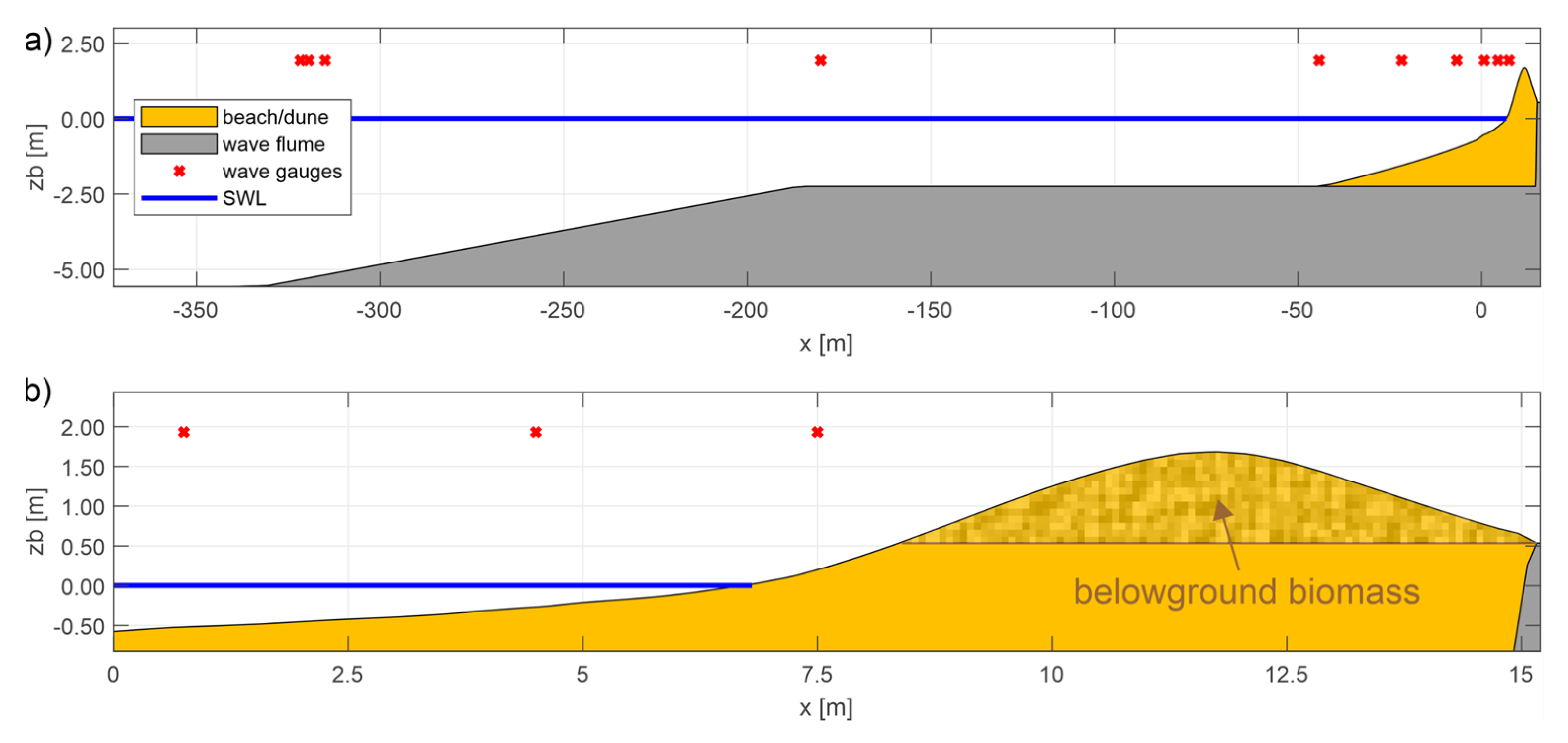
A good example of XBeach large-scale modeling is the application to Deltaflume test T04, which was also used for initial calibration of the XBeach model (see Roelvink et al. [17] for the details). A small dune with a height of approx. 1.65 m was located in front of a larger dune and eroded due to collision and overwash [35]. Within the scope of this study, it was therefore chosen to upscale the small-scale 1D-model used in Schweiger and Schuettrumpf [32] to match the dune dimensions of Deltaflume test T04. From the initial small-scale dune height of hD = 0.223 m above still water level follows an increase in height by approximately a factor of SF ~ 15/2 = 7.5 = nh. Applying an equal length ratio (nl = 7.5) results in a geometrical undistorted model (ng = 1).
The upscaled 1D-model with a length of approximately 475 m is shown in Figure 2. The origin of the local coordinate system equals the starting point of profile measurements (x = 0 m) and the initial lower water level (zb = 0 m), which was 225 cm above the flume floor (see Table 1). To reduce the computational cost, a fast 1D (ny = 0) non-equidistant grid was generated with dxmax = 10 m at the offshore boundary and a minimal grid size of dxmin = 0.1 m in the beach-dune area, which was chosen based on preliminary testing (nx = 253). The model setup was similar to that in Schweiger and Schuettrumpf [32]. Among others, spatially varying friction coefficients (Manning) were applied with n = 0.03 s/m1/3 in the sandy section of the flume. For the concrete section, a Manning coefficient of n = 0.01 s/m1/3 was used and hard structures enabled. With respect to sediment characteristics, grain size scaling would result in a medium diameter of D50 = 0.46 mm (Equation (9)). However, the initial value of D50 = 0.15 mm was maintained due to the general sediment scaling issues mentioned before (see Section 2.3).
The four different hydrodynamic boundary conditions (shallow collision (SC1), shallow overwash (SO), deep collision (DC) and deep overwash (DO)) were scaled according to Froude. While the constant water levels (tideloc = 0) and Hm0 wave heights were scaled by SF = 7.5, the peak wave period Tp and the duration of each wave burst were scaled according to SF−0.5. The wave boundary conditions were applied as JONSWAP spectra (γ = 3.3) with rt (duration of each spectrum at the offshore boundary) equaling the duration of one wave burst. The resulting simulation times were tstop = 1,100 s for DO (only one wave burst), tstop = 3,300 s for SO and tstop = 9,900 s for the C-conditions. Similarly to the application to small-scale, the default spin-up time of wave boundary conditions was reduced from taper = 100 s to zero in order to prevent underestimation of the measured wave heights during the first wave burst [32]. An overview of the upscaled hydrodynamic boundary conditions is given in Table 1.
3. Results
3.1. Hydrodynamic Calibration
The model was hydrodynamically calibrated (morphology = 0) by comparing the upscaled measured Hrms,hf wave heights of each wave burst with the time-averaged spatial output Hmean over one wave burst (tintm = rt). The XBeach default settings were applied with gamma = 0.5, and thus, the same settings as for the small-scale applications [32]. Varying the breaker index between 0.45 < γ < 0.7 did not improve the overall results, so that a value of gamma = 0.5 was used for the remainder of the investigation. Figure 3 shows the comparison of Hrms.hf wave height for conditions SC1 (a), SO (b), DC (c) and DO (d) along the wave flume for each wave burst and the scatter, the coefficients of determination (R2) and the bias (Figure 3e) for gamma = 0.5.
The comparison with the upscaled measured Hrms,hf wave heights shows good overall agreement for each hydrodynamic condition, with the bias varying between −0.3 cm (DC) and 5.77 cm (SO). The most agreement with the observation was achieved for the overwash cases with R2 = 0.78 for SO and R2 = 0.82 for DO. With respect to nearshore wave heights, the model underestimated the maximum observed wave height, except for SO. Overall, the results are very well in line with the model’s small-scale application [32], as similar statistics were derived (see Table 2), which proves that the translation to a larger scale is valid with respect to hydrodynamics.
3.2. Morphodynamic Calibration
The morphodynamic calibration was performed based on the upscaled control cases and by reusing the boundary conditions generated during the hydrodynamic calibration (wbctype = reuse). Due to the similar model performance in small-scale and large-scale situations in terms of hydrodynamics, the final morphodynamic parameter settings of Schweiger and Schuettrumpf [32] were used as initial settings in this study; and the critical avalanching slopes were set to wetslp = 0.2 and dryslp = 0.7. However, the depthscale parameter was set to SF = 2 to be consistent with the upscaled model setup (1:2). As a result, the effected morphodynamic parameters were reduced to eps = 0.0025 m (threshold water depth above which cells are wet), hmin = 0.1 m (threshold water depth for Stokes drift), hswitch = 0.05 m (switched from wet to dry) and dzmax = 0.05 m/s/m (maximum bed-level change due to avalanching).
The morphodynamic calibration was performed by comparing the final dune profiles and the percentages of deviation in post-dune volume per meter (ΔV), which was calculated for both measurements and the simulation for the area above the concrete wall (zb > 0.54 m). Furthermore, the Brier skill score (BSS) was calculated:
with zbc being the computed bed level, zbm the measured bed level and zb0 the initial bed level. The BSS defines a model skill as bad (<0), poor (0–0.3), fair (0.3–0.6), good (0.6–0.8) or excellent (0.8–1) according to the classification of van Rijn et al. [48].
Figure 4 shows the initial (dotted) and the final measured (dashed) dune profiles for each hydrodynamic condition (a–d) in combination with various simulation results (colored dash-dotted). Applying the initial settings (blue lines) led to an overprediction of the observed dune erosion for each hydrodynamic condition which was greater for the conditions targeting collision (Figure 4a,c). Similarly to the small-scale application, however, no overwash was computed for each hydrodynamic condition, which is contrary to initial expectations due to the large-scale application. Since the aim of this study was to validate the root model for large-scale and overwash in particular, we chose to induce the occurrence of overwash by additionally varying hydrodynamic parameters, although the model was already hydrodynamically calibrated.
Therefore, various hydrodynamic parameters were additionally considered in order to induce overwash. The majority of these parameters (e.g., alpha (wave dissipation coefficient): 0.5–2; gammax (maximum ratio wave height to water depth): 2, 3; n (power in Roelvink dissipation model): 10, 15), and other processes (swrunup (short-wave runup): 1 with facrun = 2) had a negligible effect on the results. However, increasing the delta (δ) parameter resulted in the occurrence of overwash for SO and DO. This parameter, which is zero by default, defines the fraction of Hrms wave height that is added to the water depth h within the calculation of the maximum wave height Hmax:
where γ is the breaker index. While overwash was observed for delta ≥ 0.5, a final value of delta = 0.7 was chosen due to the highest agreement with the post-observed dune crest height for SO. In addition, applying delta = 0.7 reduced the erosion at the dune front for all hydrodynamic conditions (Figure 4a–d, yellow). However, the downside of adjusting the delta parameter is a decrease in model accuracy concerning nearshore wave heights, which is reflected by the wave statistics in Table 3. In favor of accurately modeling the relevant overwash conditions, we chose to use a value of delta = 0.7 in the remainder of the investigation. The reason for this was that the validation of the root model for a large-scale application was based on the comparison of the belowground with the respective control cases. Thus, deviations in terms of hydrodynamics were assumed to apply to both cases equally.
In order to further decrease the erosion at the dune front, the facua parameter was increased to 0.3 (Figure 4, orange lines), which promotes the effect of wave skewness and asymmetry on the sediment advection velocity, and hence increases the onshore-directed sediment transport [49]. However, there was still too much erosion at the dune front for each hydrodynamic condition. Therefore, the increase to facua = 0.3 was combined with delta = 0.7, which further improved the results (Figure 4, purple). For the C-conditions, erosion at the dune front decreased and the computed dune face was in line with the observation for SC1. With respect to statistics (see Table 4), however, model skill remained low (BSSSC1 < −1, BSSDC = −0.24), although the deviation in post-volume decreased considerably from −152% to −32.9% (SC1) and from −98% to 4.1% (DC). For the conditions targeting overwash, the computed post-dune crest heights are in good agreement with the measurements. Nevertheless, low skill was achieved for SO (BSS < −1), although the deviation in post-volume decreased from −78.9% to −4.5%. For DO, however, the final dune profile shape is very well in line with the observation, which demonstrates excellent model skill (BSS = 0.88). The deviation in post-volume (14.6%) can be attributed to the general model–data mismatch between 3 m < x < 9 m (d).
3.3. Modeling Aboveground and Belowground Vegetation Cases
In order to model the effect of BGB on dune erosion volumes at large scales, the upscaled belowground cases of Bryant et al. [34] served as comparative examples, where uniformly integrated coconut husk fibers represented belowground biomass. Within the scope of this study, it was hence assumed that the influence of these fibers on the erosion resistance of the soil scales linearly with the model setup. Therefore, it was assumed that the comparison of the simulation results with the upscaled measured final dune profiles (BGB) would be valid, as would the comparison of the dune profile differences (BGB to control).
Due to the inconsistent model performance during calibration in the collision and overwash conditions, the modelling of the belowground cases was performed separately. For the C-conditions, only the constant (with respect to rcc value) root model was applied with a constant and a locally varying rooting depth (zroot). Due to the non-occurrence of overwash in the control simulations, locally increased friction coefficients were not considered. For the O-conditions, however, both the constant root model (with constant/varying zroot) and the friction approach were considered in the simulation. In general, the root model was applied with a maximum rooting depth of zroot = 1.15 m, which equals the difference between the dune crest and the height of the sloping wall. In the case of local variation, the rooting depth was defined as the difference between the initial dune profile and the height of the concrete wall (zb = 0.54 m), which was provided for each grid cell through an external file (see Figure 1).
Since locally increasing the bed friction coefficients is the common practice for the consideration of aboveground vegetation in (XBeach) modeling [22,27,28,29,50], the aboveground cases (AGB) of Bryant et al. [34] served as an additional source of comparison when solely using the friction approach. In the physical experiment, aboveground biomass was represented by 30.5 cm long wooden dowels which were buried half of their length deep. Finally, the combination of the root model and locally increased friction coefficients was compared to the upscaled above and belowground cases (ABGB) of Bryant et al. [34]. In this regard, it should be noted that there was no physical connection between the wooden dowels (ABG) and the husk fibers (BGB) in the physical experiment.
3.3.1. Collision Regime
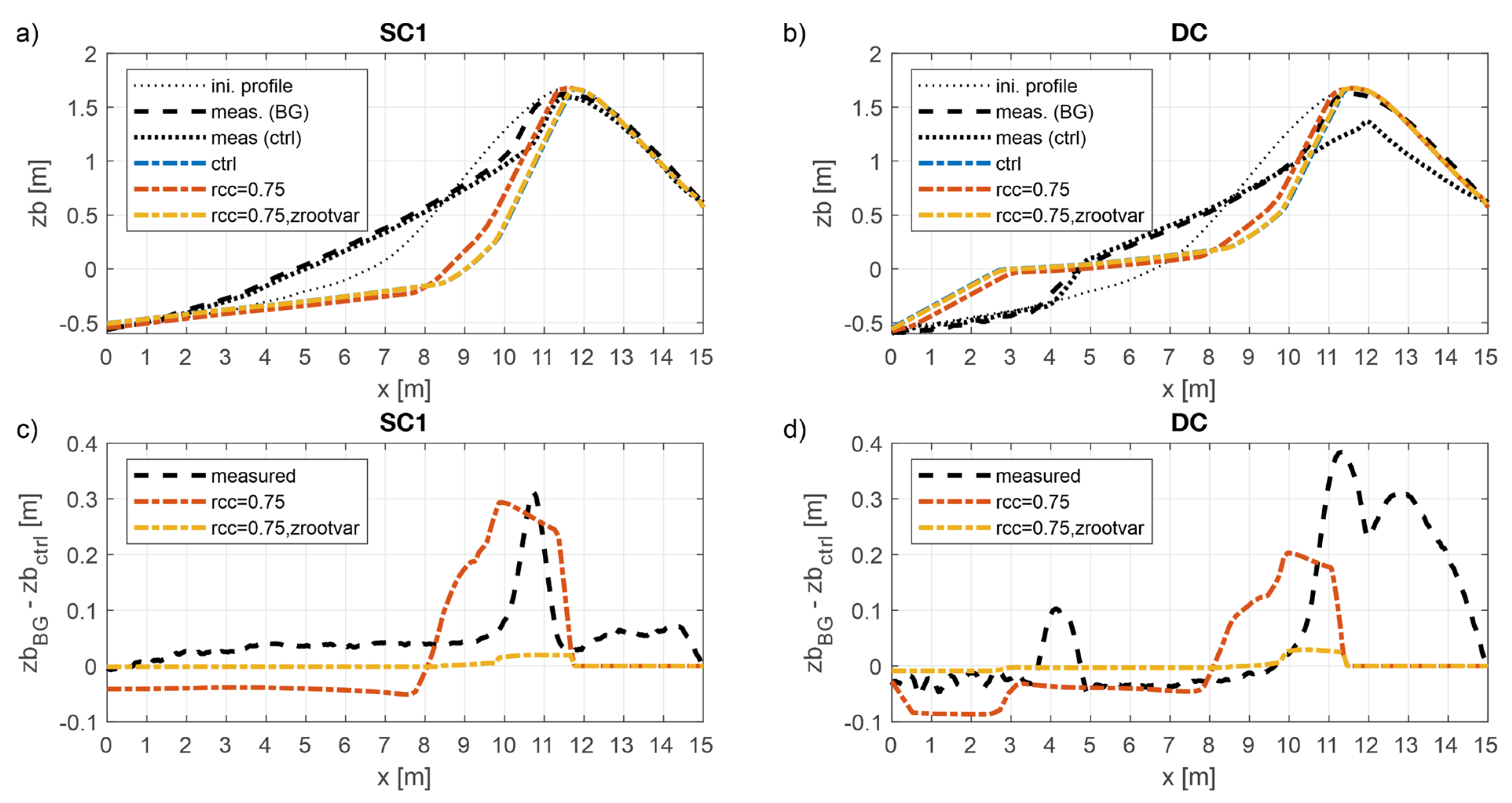
Applying the root model to the belowground cases of the conditions targeting collision decreased the dune erosion at the dune front for both SC1 and DC. However, the influence of the root model remained constant for rcc ≥ 0.75. As an example, Figure 5 shows the final dune profiles of the measurements (black), the control simulation (blue) and when applying the root model with rcc = 0.75 and a constant (orange) or a spatially varying rooting depth (yellow) for SC1 (a) and DC (b). Given as well are the dune profile differences between belowground and control for SC1 (c) and DC (d). In the case of SC1, using the root model with constant zroot resulted in a similar maximum decrease of Δzbmax = 30 cm as the measurement. However, the location of maximum decrease was shifted offshore by one meter and erosion at the dune front (8 m < x < 10 m) was too high in comparison to the upscaled measurement (c). The use of spatially varying rooting depths to decrease the influence of the root model at the dune face had only a minor effect with respect to the control. For DC, similar results can be observed. However, the model predicted a maximum decrease of Δzbmax = 20 cm, which is much lower than the upscaled measurement with Δzbmax = 40 cm (d).
3.3.2. Overwash Regime
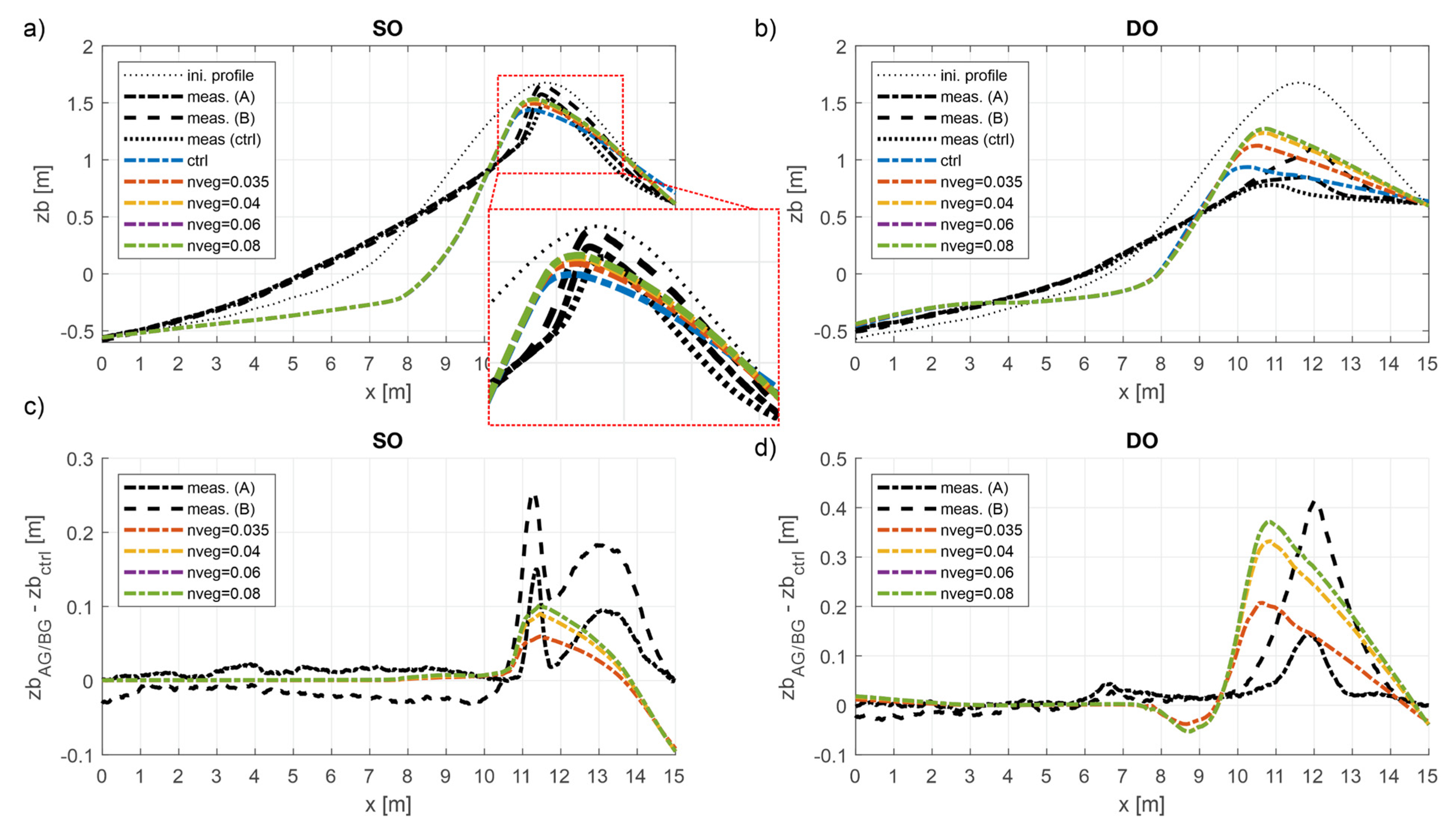
Due to the occurrence of overwash in the control simulations, the use of locally increased friction coefficients was considered in the modeling of the O-conditions. In this regard, the friction coefficients were locally increased between 0.035 s/m1/3 and 0.08 s/m1/3 (shrubs [28]). Figure 6 shows the simulation results, including the final dune profiles for SO (a) and DO (b) and the dune profile differences (c, d). In general, increasing the bed friction coefficients decreases the erosion on the lee side of the dune. While the measured maximum decrease in erosion (x = 11.4 m) was underestimated by 15 cm for SO when using nveg = 0.08 s/m1/3 (c, green), the maximum decrease of Δzbmax = 37 cm for DO (d, green) is in good agreement with the upscaled measurement (Δzbmax = 41 cm), but shifted offshore by 1.25 m.
With respect to AGB, the maximum decrease in erosion at x = 11.4 m was underestimated by approximately 5 cm when applying nveg ≥ 0.06 s/m1/3(green and purple). For DO, however, the effect of aboveground biomass on dune erosion volumes was overestimated for nveg ≥ 0.035 s/m1/3.
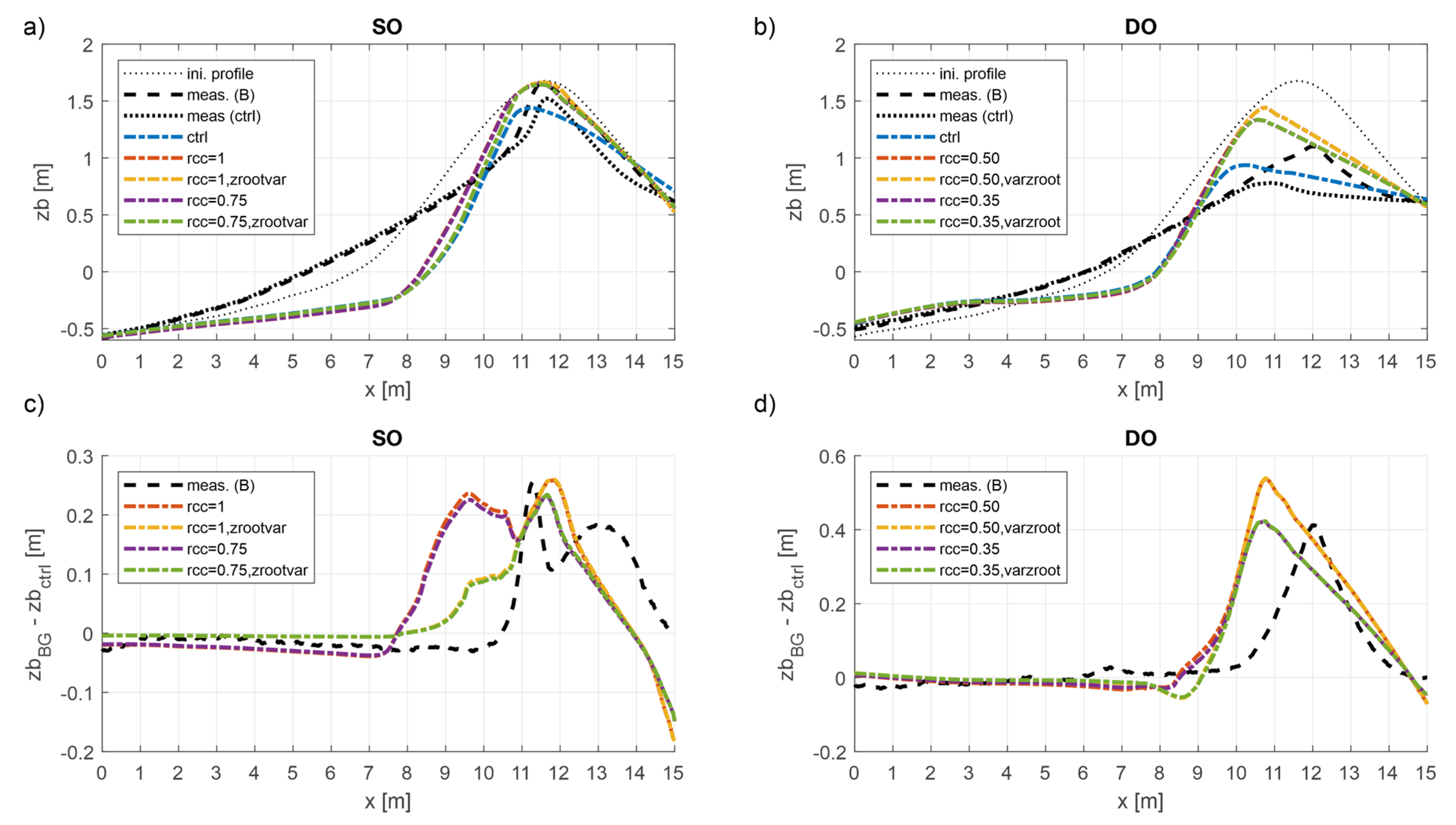
Applying the root model led to results that differed with the overwash conditions and with the use of constant or spatially varying rooting depth. Figure 7 summarizes different final dune profiles (a, b) and dune profile differences (c, d) for different root model configurations compared to the upscaled measured data. For SO, using rcc values of 0.75 and 1 resulted in good agreement between the model and the measurements with respect to the maximum decrease (x = 11.5 m) in the presence of BGB (c). Furthermore, incorporating a spatially varying rooting depth decreased the effect of the root model on the model predicted erosion at the dune front (x < 11 m) in comparison to the simulations with a constant rooting depth (orange, purple). As a result, greater agreement with the measurements was achieved. For the back of the dune (x > 12 m), however, the predicted decrease in dune erosion was lower than the measurement. For DO, the best agreement with respect to dune profile differences between BGB and control was achieved for rcc = 0.35 (d). Although the location of maximum decrease was shifted by approximately 1.5 m offshore, the general profile shape was in good agreement with the observations of the front and the back of the dune. Contrary to the application to SO, the use of a spatially varying rooting depth led to only minor differences in the dune foot area (8 m < x < 9 m).
Despite the comparison of dune profile differences, the overwash sediment volumes per meter width (Vover) were calculated for each simulation:
Subsequently, the percentage decrease in overwash volume in each control simulation was derived to enable a comparison to the results of the small-scale physical experiment [34]. It should be noted that the latter were obtained by collecting and weighing the overwash sediment and are hence based on total sediment mass.
The ratios between BGB and control are summarized in Table 5 for shallow-overwash and in Table 6 for deep-overwash. For shallow-overwash, the presence of ABG and BGB reduced the overwash volume by 34% (37.6 kg to 24.9 kg) and by 58% (37.6 kg to 15.9 kg) in the physical experiment, respectively. The best agreement with the BGB measurement was achieved when applying the root model with rcc = 0.75 with a percentage decrease of 59% (const. zroot) and 60% (var. zroot). In case of the former, this corresponds to a decrease from 0.58 m3/m to 0.24 m3/m. Hypothetically, the observed decrease in overwash sediment mass of (37.6–15.9) kg = 21.7 kg would be equivalent to an upscaled decrease in overwash volume of 0.04 m3/m (the translated overwash volume follows from Vover = 21.7 kg/2650 kg/m3/1.5 m·7.5 = 0.041 m3/m) when assuming a sediment density of 2650 kg/m3 (XBeach default), and when using the small-scale flume width of 1.5 m and the scale factor of 7.5. Thus, the model theoretically overpredicts the decrease in overwash volume by a factor of 8.5 (= (0.58−0.24)/0.04). For AGB, the use of locally increased friction coefficients underestimates the measured percentage decrease in overwash volume by at least 5% (nveg ≥ 0.06 s/m1/3).
For DO, the presence of AGB decreased the total overwash sediment mass by 20% from 144.2 kg to 115.5 kg. For BGB, the total overwash sediment decreased to 78 kg (46%). As an example, the theoretical upscaling for BGB resulted in an overwash volume decrease of 0.12 m3/m for the measurement. With respect to modeling, the greatest agreement was achieved when applying the root model with rcc = 0.35 and a variable rooting depth. Then, the predicted overwash volume decreased by 43% from 2.49 m3/m to 1.41 m3/m. The theoretical comparison between the model and the upscaled measurements found overestimation by a factor of 9 (= (2.49−1.41)/0.12). Concerning locally increased friction, using values of n ≥ 0.06 s/m1/3 led to a decrease in overwash volume by 41%, and hence, similar (good) agreement with the measurements.
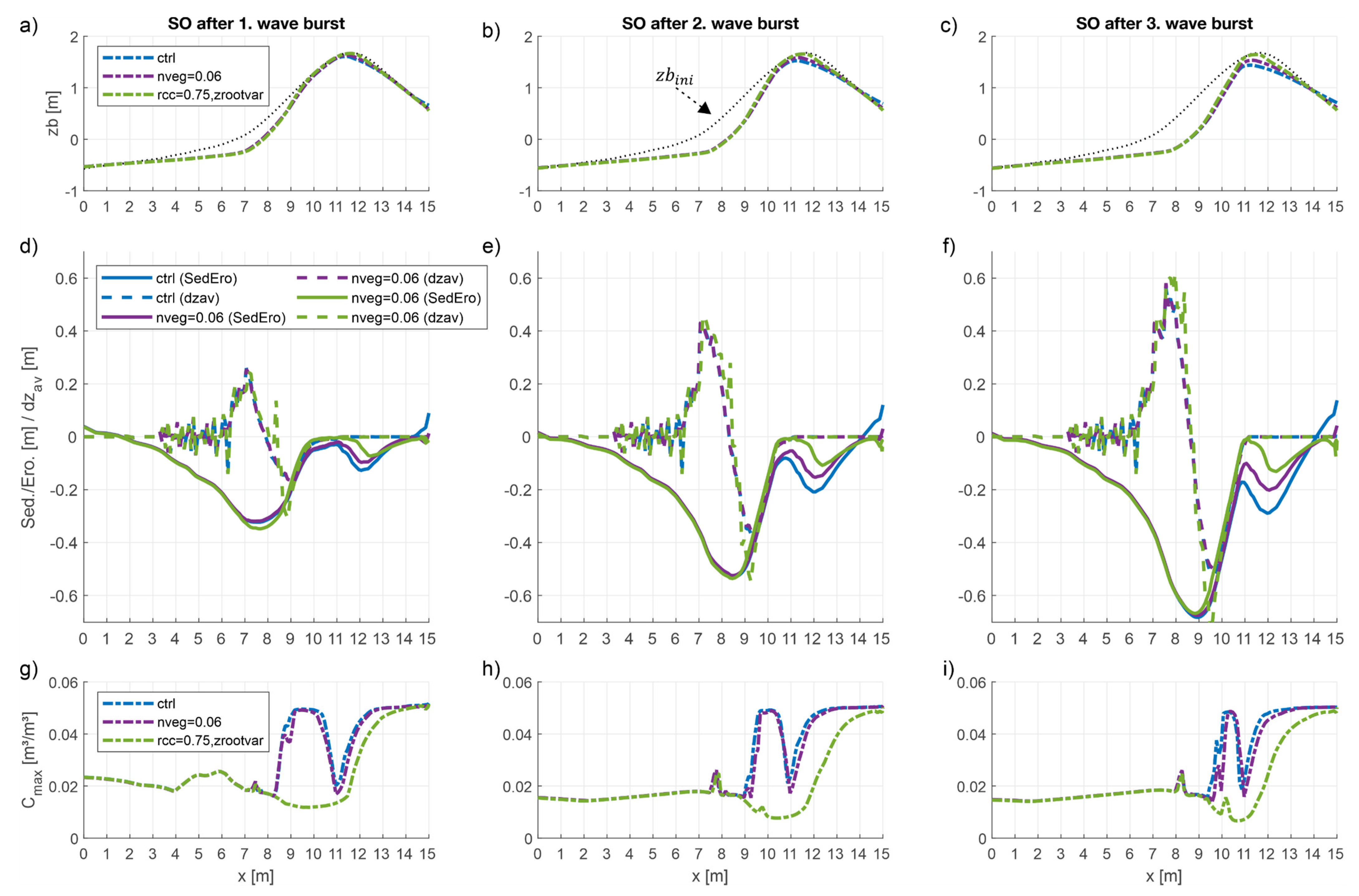
Further analysis was conducted by evaluating the root model (rcc = 0.35, var. zroot) and using locally increased friction coefficients (nveg = 0.06 s/m1/3) for SO after each wave burst. Figure 8 presents the dune profiles (a−c), the cumulative erosion and the bed-level changes due to avalanching (d−f) and the maximum sediment concentration during each wave burst (g−i). After the first wave burst, erosion at the dune crest (x = 11.5 m) was greatest for the control simulation (blue) with a decrease of Δzbwb1,ctrl = −8 cm (d). Locally increasing the bed friction (purple) reduced erosion at the dune crest to Δzbwb1,fric = −5 cm. With the root model (green), erosion at the dune crest was almost prevented (Δzbwb1,rm < −1 cm). As a result, the cumulative erosion on the lee side of the dune was greatest for the control simulation with a maximum bed level change of Δzbwb1,ctrl = −12 cm at x = 12 m, which decreased to Δzbwb1,fric = −10 cm (friction) or Δzbwb1,rm = −7 cm (root model). The results show further that there is no contribution of avalanching for x > 11.2 m (dzav = 0). With respect to the maximum sediment concentration, only small differences can be observed between the control and the friction approach. Applying the root model reduced the maximum sediment concentration at both the front (9 m < x < 11.5 m) and the back of the dune.
In the remainder of the control simulation, erosion at the dune crest and on the lee side of the dune increased to a maximum of Δzbwb2,ctrl = −21 cm after the second wave burst (e) and Δzbwb3,ctrl = −28 cm after the third wave burst (f). For locally increased friction and the root model, the maximum erosion decreased to Δzbwb2,fric = −15 cm and Δzbwb3,fric = −20 cm (friction), and to Δzbwb2,rm = −10 cm and Δzbwb3,rm = −12 cm (root model). In terms of maximum sediment concentrations, similar results as for the first wave burst were obtained when using locally increased friction (similar to control) and the root model (lower than control), which also applies to the non-occurrence of avalanching for x > 11.2 m. In summary, using the root model and thus increasing the critical velocity for erosion along the dune reduced the overall erosion, especially at the dune crest. As a result, erosion on the lee side of the dune was reduced during the second and third wave bursts without bed level changes due to avalanching, which finally resulted in lower overwash sediment volumes (see Table 5).
3.4. Modeling the Combination of Aboveground and Belowground Vegetation
Due to the occurrence of overwash and thus an influence of locally increased friction coefficients on the predicted erosion volumes, further simulations were conducted by using both the root model and locally increased friction coefficients. In this way, the root model was applied with varying rooting depth and with rcc = 0.75 for SO and rcc = 0.35 for DO based on the BGB modeling (see Figure 7). The results were compared to the upscaled ABGB results of Bryant et al. [34].
Figure 9 presents the final dune profiles for SO (a) and DO (b) and the dune profile differences between ABGB and the control (dash-dotted), and between the simulation and the measurements (dotted in (c) and (d)). Furthermore, the percentage decreases in sediment loss to overwash are summarized in Table 7. In general, the comparison of final dune profiles (a, b) shows that combining the two approaches decreased dune erosion volumes on the lee side of the dune compared to using the root model alone (orange). For SO, the combination of the root model with locally increased friction coefficients to nveg = 0.08 s/m1/3 underpredicted the upscaled measured decrease due to the presence of ABGB (c). Nevertheless, the final dune profile is in good agreement with the measurement for x > 11.3 m, as shown by the differences between simulation and measurement (dotted line in c). However, the observed decrease in overwash volume (86%) was underpredicted by 11%.
While for DO, the root model resulted in good agreement with the upscaled BGB measurement (see Figure 7), the local increase of friction coefficients overpredicted the effect of AGB with nveg = 0.035 s/m1/3 (see Figure 6). Concerning ABGB, however, combining the root model (rcc = 0.35) with locally increased friction coefficients underpredicted the measured decrease in dune erosion volume, even for nveg = 0.08 s/m1/3 (Figure 9d). Furthermore, only minor errors occurred in the simulations using both the root model and the friction approach. This also applies to the percentage decrease in sediment loss to overwash, which was 20% (nveg = 0.035 s/m1/3) to 18% (nveg = 0.08 s/m1/3) lower than observed in the physical experiment (83%). In order to increase the effect of the root model, combining rcc = 0.5 with a local friction value of nveg = 0.08 s/m1/3 resulted in good agreement with respect to dune profile differences (d) and increased the percentage decrease in overwash volume to 70.4%.
4. Discussion and Conclusions
Due to a general model–data mismatch in small-scale applications [32], this study aimed to validate the root model at larger scale based on an upscaled model setup of Bryant et al. [34]. It was expected that the overall performance and especially the predictions of overwash would improve, since XBeach’s default parameters are optimized for large-scale modeling. With respect to Hrms,hf wave heights, good agreement was achieved between the model and (upscaled) measurements for each hydrodynamic condition. Similarly to the small-scale application, dune overwash was not computed regardless of the hydrodynamic condition, which did not change when activating short-wave runup. Only the increase of the delta parameter, and thus, the maximum wave height in the nearshore zone, resulted in the occurrence of dune overwash for the O-conditions. From this follows that the general model–data mismatch described in Schweiger and Schuettrumpf [32] might not only result from the small-scale application, but might (also) be due to other model inaccuracies, such as an underestimation of wave runup, as discussed in previous studies [51,52,53].
Although adjustments to various model parameters were considered in the morphodynamic calibration, erosion volumes at the font of the dune were significantly overestimated for all conditions except DO (see Figure 4). As a result, low model skill was achieved for SC1, DC and SO (BSS < 0), whereas an excellent skill was achieved for DO (BSS = 0.88). However, the overestimated erosion at the dune face and toe is in line with the findings of van Dongeren et al. [54], who, among others, observed an overprediction of erosion around the mean waterline, possibly due to inaccuracies in the modeling of sediment motion in the swash zone (see also [53,55]). In this study, the overestimation of erosion at the dune toe could have been further reduced by further increasing the facua parameter, which promotes the onshore-directed sediment transport. However, this would have been followed by an increasing deviation of the dune front position between the model and measurements, which was already observed for SO when applying facua = 0.3 with delta = 0.7 (see Figure 4b). Therefore, deviations at the dune front were accepted since the main focus in this study was on the erosion at the dune crest and on the lee side of the dune due to overwash.
The effects of locally increased friction coefficients and the root model on dune erosion volumes at a large scale were validated by using the upscaled biomass cases (AGB, BGB, ABGB) of Bryant et al. [34] as a reference. Therefore, a major assumption in this study was that the effects of the wooden dowels (AGB), the husk fibers (BGB) and their combination (ABGB) on the erodibility of the sandy soil scale linearly with the translation to a large scale. From this follows that the validation of two approaches to consider land-based biomass in this study was not based on real data from a physical experiment but relied on a theoretical comparison. Nevertheless, applying the root model to the O-conditions resulted in good agreement with the upscaled BGB measurements, which was better when spatially varying rooting depths were applied. However, the best results for SO and DO were achieved with different rcc values. While for SO a value of rcc = 0.75 led to good agreement concerning dune profile differences (BGB to control), the application to DO required a reduction to rcc = 0.35. Although these results are based on a theoretical comparison, the effect of the root model on the model predicted erosion should be consistent and independent of the hydrodynamic conditions. Therefore, further investigations are necessary to improve the performance of the root model. Due to a lack of appropriate data concerning the interaction between belowground biomass and sandy soil, future studies should focus on quantifying the effects of land-based (belowground) biomass on the erodibility of a dune system, as suggested by Figlus et al. [33]. With respect to further validating the root model in XBeach, these studies should be conducted at a large scale and additionally consider real dune vegetation.
Using locally increased friction coefficients decreased the dune erosion volumes on the lee side of the dune. Concerning BGB modeling, using a local friction coefficient of nveg = 0.08 s/m1/3 underestimated the decrease in erosion, which was greater for SO (see Figure 6). Since the friction approach is the common practice for considering the effect of land-based vegetation on overwash-dominated erosion in (XBeach) modeling [22,27,28,29,50], the results were also compared to the AGB cases. For DO, the predicted decrease in erosion was already overestimated for nveg = 0.035 s/m1/3. For SO, however, the influence of AGB on dune erosion volumes was underestimated even when using the maximum value (nveg = 0.08 s/m1/3) that was considered in this study. Therefore, the dynamic roughness module [30], which varies the Manning roughness in vegetated areas due to burying and erosion, was not considered in this study. Since the BGB measurements were underestimated when using the friction approach (see Figure 6c,d), the greater effect of ABGB on the dune erosion volumes would presumably have led to an even greater underestimation.
Nevertheless, the combination of the root model with locally increased friction coefficients was validated with the upscaled ABGB measurements. Due to the good performance in the BGB modeling (root model with rcc = 0.35) and the overestimation observed in the AGB modeling for DO (friction approach), combining the two approaches was expected to result in good agreement with the ABGB measurements for DO. Although less erosion was predicted on the lee side of the dune in comparison to the sole use of the root model, the overall decrease due to the presence of ABGB was lower in comparison to the upscaled measurement and less sensitive to variations in local bed friction (see Figure 9d). In this regard, increasing the rcc value to 0.5 resulted in a good agreement between model and upscaled measurements. This necessary increase could be attributed to the general model setup, where the wooden dowels were buried half way. Thus, the belowground parts of the dowels could have further increased the resistance of the dune in addition to the effect of the uniformly integrated coir fibers, hence requiring a higher contribution of the root model, and hence, higher rcc values.
In summary, the application of the XBeach model to an upscaled model setup of Bryant et al. [34] showed a general model–data mismatch for all hydrodynamic conditions except for DO, which was mainly due to overestimated dune erosion volumes around the initial waterline. Nevertheless, applying the root model to the upscaled BGB cases reduced the predicted dune erosion for all hydrodynamic conditions. In this regard, incorporating spatially varying rooting depths further improved the results at the dune front, although the overall effect of the root model differed between the simulations. However, there is a lack of appropriate data to further validate and improve the root model. Although various wave flume experiments have been conducted in recent years, there is a specific need for research focusing on the effect of land-based biomass on the erodibility of dunes during collision and overwash at large scales. In particular, the separate investigation of aboveground and belowground biomass concerning wave-induced dune erosion at large scales and the individual contributions of different plant characteristics (e.g., rooting depth, plant/root density and maturity) would allow one to evaluate the specific influences of these plant-related parameters on the erosive processes. Furthermore, these studies should additionally address the effects of land-based vegetation on the temporal evolution of dune scarping, avalanching and failure.
Author Contributions
Conceptualization, C.S.; methodology, C.S.; software, C.S.; validation, C.S.; formal analysis, C.S.; investigation, C.S.; resources, H.S.; data curation, C.S.; writing—original draft preparation, C.S.; writing—review and editing, H.S.; visualization, C.S.; supervision, H.S.; project administration, H.S.; funding acquisition, H.S. Both authors have read and agreed to the published version of the manuscript.
Funding
This research was funded by the German Federal Ministry of Education and Research (BMBF) within the project PADO (grant number: 03F0760A) that was initiated in the framework of the German Coastal Engineering Research Council (KFKI).
Institutional Review Board Statement
Not applicable.
Informed Consent Statement
Not applicable.
Data Availability Statement
The data used in this study are available from the corresponding author.
Acknowledgments
The authors would like thank Mary A. Bryant and Duncan B. Bryant (U.S. Army Engineer Research and Development Center, Vicksburg, USA) for providing the data of their small-scale wave flume experiment. Furthermore, the authors want to thank the anonymous reviewers for their feedback, which helped to improve the quality of this manuscript.
Conflicts of Interest
The authors declare no conflict of interest. The funders had no role in the design of the study; in the collection, analyses or interpretation of data; in the writing of the manuscript, or in the decision to publish the result.
References
- Martínez, M.L.; Psuty, N.P.; Lubke, R.A. A Perspective on Coastal Dunes. In Coastal Dunes; Caldwell, M.M., Heldmaier, G., Jackson, R.B., Lange, O.L., Mooney, H.A., Schulze, E.-D., Sommer, U., Martínez, M.L., Psuty, N.P., Eds.; Springer Berlin Heidelberg: Berlin/Heidelberg, Germany, 2008; pp. 3–10. ISBN 978-3-540-74001-8. [Google Scholar]
- Everard, M.; Jones, L.; Watts, B. Have we neglected the societal importance of sand dunes? An ecosystem services perspective. Aquat. Conserv. Mar. Freshw. Ecosyst. 2010, 20, 476–487. [Google Scholar] [CrossRef]
- Temmerman, S.; Meire, P.; Bouma, T.J.; Herman, P.M.J.; Ysebaert, T.; de Vriend, H.J. Ecosystem-based coastal defence in the face of global change. Nature 2013, 504, 79–83. [Google Scholar] [CrossRef] [PubMed]
- Schoonees, T.; Gijón Mancheño, A.; Scheres, B.; Bouma, T.J.; Silva, R.; Schlurmann, T.; Schüttrumpf, H. Hard Structures for Coastal Protection, Towards Greener Designs. Estuaries Coasts 2019, 42, 1709–1729. [Google Scholar] [CrossRef]
- Vriend, H.J.; van Koningsveld, M.; Aarninkhof, S.G.; Vries, M.B.; Baptist, M.J. Sustainable hydraulic engineering through building with nature. J. Hydro-Environ. Res. 2015, 9, 159–171. [Google Scholar] [CrossRef]
- Barbier, E.B.; Koch, E.W.; Silliman, B.R.; Hacker, S.D.; Wolanski, E.; Primavera, J.; Granek, E.F.; Polasky, S.; Aswani, S.; Cramer, L.A.; et al. Coastal ecosystem-based management with nonlinear ecological functions and values. Science 2008, 319, 321–323. [Google Scholar] [CrossRef] [PubMed]
- Feagin, R.A.; Lozada-Bernard, S.M.; Ravens, T.M.; Möller, I.; Yeager, K.M.; Baird, A.H. Does vegetation prevent wave erosion of salt marsh edges? Proc. Natl. Acad. Sci. USA. 2009, 106, 10109–10113. [Google Scholar] [CrossRef] [PubMed] [Green Version]
- Rosati, J.D.; Stone, G.W. Geomorphologic Evolution of Barrier Islands along the Northern, U.S. Gulf of Mexico and Implications for Engineering Design in Barrier Restoration. J. Coast. Res. 2009, 251, 8–22. [Google Scholar] [CrossRef]
- Lindell, J.; Hallin, C.; Hanson, H. Impact of dune vegetation on wave and wind erosion A case study at Ängelholm Beach, South Sweden. VATTEN J. Water Manag. Res. 2017, 73, 39–48. [Google Scholar]
- Feagin, R.A.; Furman, M.; Salgado, K.; Martinez, M.L.; Innocenti, R.A.; Eubanks, K.; Figlus, J.; Huff, T.P.; Sigren, J.; Silva, R. The role of beach and sand dune vegetation in mediating wave run up erosion. Estuar. Coast. Shelf Sci. 2019, 219, 97–106. [Google Scholar] [CrossRef]
- Jackson, D.W.; Costas, S.; González-Villanueva, R.; Cooper, A. A global ‘greening’ of coastal dunes: An integrated consequence of climate change? Glob. Planet. Chang. 2019, 182, 103026. [Google Scholar] [CrossRef]
- Konlechner, T.M.; Kennedy, D.M.; O’Grady, J.J.; Leach, C.; Ranasinghe, R.; Carvalho, R.C.; Luijendijk, A.P.; McInnes, K.L.; Ierodiaconou, D. Mapping spatial variability in shoreline change hotspots from satellite data; a case study in southeast Australia. Estuar. Coast. Shelf Sci. 2020, 246, 107018. [Google Scholar] [CrossRef]
- Vousdoukas, M.I.; Mentaschi, L.; Voukouvalas, E.; Verlaan, M.; Jevrejeva, S.; Jackson, L.P.; Feyen, L. Global probabilistic projections of extreme sea levels show intensification of coastal flood hazard. Nat. Commun. 2018, 9, 2360. [Google Scholar] [CrossRef] [Green Version]
- Hunter, J. Estimating sea-level extremes under conditions of uncertain sea-level rise. Clim. Chang. 2010, 99, 331–350. [Google Scholar] [CrossRef]
- Church, J.; Clark, P.; Cazenave, A.; Gregory, J.; Jevrejeva, S.; Levermann, A.; Merrifield, M.; Milne, G.; Nerem, R.; Nunn, P.; et al. Contribution of Working Group I to the Fifth Assessment Report of the Intergovernmental Panel on Climate Change. Sea Level Chang. In Climate Change 2013: The Physical Science Basis; IPCC: Geneva, Switzerland, 2013; pp. 1138–1191. [Google Scholar]
- Vitousek, S.; Barnard, P.L.; Fletcher, C.H.; Frazer, N.; Erikson, L.; Storlazzi, C.D. Doubling of coastal flooding frequency within decades due to sea-level rise. Sci. Rep. 2017, 7, 1399. [Google Scholar] [CrossRef]
- Roelvink, D.; Reniers, A.; van Dongeren, A.; van Thiel de Vries, J.; McCall, R.; Lescinski, J. Modelling storm impacts on beaches, dunes and barrier islands. Coast. Eng. 2009, 56, 1133–1152. [Google Scholar] [CrossRef]
- Vousdoukas, M.I.; Ferreira, Ó.; Almeida, L.P.; Pacheco, A. Toward reliable storm-hazard forecasts: XBeach calibration and its potential application in an operational early-warning system. Ocean. Dyn. 2012, 62, 1001–1015. [Google Scholar] [CrossRef]
- McCall, R.T.; van Thiel de Vries, J.; Plant, N.G.; van Dongeren, A.R.; Roelvink, J.A.; Thompson, D.M.; Reniers, A. Two-dimensional time dependent hurricane overwash and erosion modeling at Santa Rosa Island. Coast. Eng. 2010, 57, 668–683. [Google Scholar] [CrossRef]
- Van Ormondt, M.; Nelson, T.R.; Hapke, C.J.; Roelvink, D. Morphodynamic modelling of the wilderness breach, Fire Island, New York. Part I: Model set-up and validation. Coast. Eng. 2020, 157, 103621. [Google Scholar] [CrossRef]
- Schweiger, C.; Kaehler, C.; Koldrack, N.; Schuettrumpf, H. Spatial and temporal evaluation of storm-induced erosion modelling based on a two-dimensional field case including an artificial unvegetated research dune. Coast. Eng. 2020, 161, 103752. [Google Scholar] [CrossRef]
- Nederhoff, C.M.; Lodder, Q.J.; Boers, M.; den Bieman, J.P.; Miller, J.K. Modelling the effects of hard structures on dune erosion and overwash. In Proceedings of the Coastal Sediments 2015, San Diego, CA, USA, 11–15 May 2015; Wang, P., Rosati, J.D., Cheng, J., Eds.; World Scientifi: Singapore, 2015. ISBN 978-981-4689-96-0. [Google Scholar]
- Roelvink, D.; McCall, R.; Mehvar, S.; Nederhoff, K.; Dastgheib, A. Improving predictions of swash dynamics in XBeach: The role of groupiness and incident-band runup. Coast. Eng. 2017, 134, 103–123. [Google Scholar] [CrossRef]
- Van Rooijen, A.; Van Thiel de Vries, J.; McCall, R.; van Dongeren, A.; Roelvink, D.J.; Reniers, A. Modeling of wave attenuation by vegetation with XBeach. In Proceedings of the 36th IAHR World Congress, 28 June–3 July 2015, The Hague, The Netherlands: Deltas of the Future and What Happens Upstream; IAHR: The Hague, The Netherlands, 2015; ISBN 9789082484601. [Google Scholar]
- Van Rooijen, A.; Lowe, R.; Rijnsdorp, D.P.; Ghisalberti, M.; Jacobsen, N.G.; McCall, R. Wave-Driven Mean Flow Dynamics in Submerged Canopies. J. Geophys. Res. Ocean. 2020, 125, 57. [Google Scholar] [CrossRef] [Green Version]
- Van Rooijen, A.A.; McCall, R.T.; van Thiel de Vries, J.S.M.; van Dongeren, A.R.; Reniers, A.J.H.M.; Roelvink, J.A. Modeling the effect of wave-vegetation interaction on wave setup. J. Geophys. Res. Ocean. 2016, 121, 4341–4359. [Google Scholar] [CrossRef] [Green Version]
- De Vet, P.; McCall, R.T.; den Biemann, J.P.; Stive, M.; van Ormondt, M. Modelling dune erosion, overwash and breaching at fire island (NY) during hurricane Sandy. In The Proceedings of the Coastal Sediments 2015; Wang, P., Rosati, J.D., Cheng, J., Eds.; World Scientific: San Diego, CA, USA, 2015; ISBN 978-981-4689-96-0. [Google Scholar]
- Passeri, D.L.; Long, J.W.; Plant, N.G.; Bilskie, M.V.; Hagen, S.C. The influence of bed friction variability due to land cover on storm-driven barrier island morphodynamics. Coast. Eng. 2018, 132, 82–94. [Google Scholar] [CrossRef]
- Fernández-Montblanc, T.; Duo, E.; Ciavola, P. Dune reconstruction and revegetation as a potential measure to decrease coastal erosion and flooding under extreme storm conditions. Ocean. Coast. Manag. 2020, 188, 105075. [Google Scholar] [CrossRef]
- Van der Lugt, M.A.; Quataert, E.; van Dongeren, A.; van Ormondt, M.; Sherwood, C.R. Morphodynamic modeling of the response of two barrier islands to Atlantic hurricane forcing. Estuar. Coast. Shelf Sci. 2019, 229, 106404. [Google Scholar] [CrossRef]
- Bendoni, M.; Georgiou, I.Y.; Roelvink, D.; Oumeraci, H. Numerical modelling of the erosion of marsh boundaries due to wave impact. Coast. Eng. 2019, 152, 103514. [Google Scholar] [CrossRef]
- Schweiger, C.; Schuettrumpf, H. Considering the effect of belowground biomass on dune erosion volumes in coastal numerical modelling. Coast. Eng. 2021, 168, 103927. [Google Scholar] [CrossRef]
- Figlus, J.; Sigren, J.M.; Poesen, J.; Armitage, A. Physical Model Experiment Investigating Interactions between Different Dune Vegetation and Morphology Changes under Wave Impact. In Proceedings of Coastal Dynamics 2017; Paper No. 059; pp. 470–480. Available online: https://www.semanticscholar.org/paper/PHYSICAL-MODEL-EXPERIMENT-INVESTIGATING-BETWEEN-AND-Figlus-Sigren/f44bcee71e9245a0eccb921c721d46812e6e0bb3 (accessed on 30 July 2021).
- Bryant, D.B.; Anderson, B.M.; Sharp, J.A.; Bell, G.L.; Moore, C. The response of vegetated dunes to wave attack. Coast. Eng. 2019, 152, 103506. [Google Scholar] [CrossRef]
- Van Gent, M.; van Thiel de Vries, J.; Coeveld, E.M.; Vroeg, J.H.; van de Graaff, J. Large-scale dune erosion tests to study the influence of wave periods. Coast. Eng. 2008, 55, 1041–1051. [Google Scholar] [CrossRef]
- Arcilla, A.S.; Roelvink, D.J.; O’Connor, B.A.; Reniers, A.; Jimenez, J.A. Delta flume’93 experiment. In Coastal Dynamics ’94: Proceedings of an International Conference on the Role of the Large-Scale Experiments in Coastal Research, Universitat Politècnica de Catalunya, Barcelona, Spain, 21–25 February 1994; Arcilla, A.S., Stive, M.J.F., Kraus, N.C., Eds.; American Society of Civil Engineers: New York, NY, USA, 1994; pp. 488–502. ISBN 978-0-7844-0043-2. [Google Scholar]
- Ruessink, B.G.; Miles, J.R.; Feddersen, F.; Guza, R.T.; Elgar, S. Modeling the alongshore current on barred beaches. J. Geophys. Res. 2001, 106, 22451–22463. [Google Scholar] [CrossRef]
- Galappatti, G.; Vreugdenhil, C.B. A depth-integrated model for suspended sediment transport. J. Hydraul. Res. 1985, 23, 359–377. [Google Scholar] [CrossRef]
- Soulsby, R. Dynamics of Marine Sands: A Manual for Practical Applications; Telford: London, UK, 1997; ISBN 978-0727725844. [Google Scholar]
- Van Rijn, L.C. Sediment Transport, Part III: Bed forms and Alluvial Roughness. J. Hydraul. Eng. 1984, 110, 1733–1754. [Google Scholar] [CrossRef]
- Vannoppen, W.; Baets, S.; Keeble, J.; Dong, Y.; Poesen, J. How do root and soil characteristics affect the erosion-reducing potential of plant species? Ecol. Eng. 2017, 109, 186–195. [Google Scholar] [CrossRef] [Green Version]
- De Baets, S.; Poesen, J.; Reubens, B.; Wemans, K.; Baerdemaeker, J.; Muys, B. Root tensile strength and root distribution of typical Mediterranean plant species and their contribution to soil shear strength. Plant Soil 2008, 305, 207–226. [Google Scholar] [CrossRef]
- Van Rijn, L.C.; Tonnon, P.K.; Sánchez-Arcilla, A.; Cáceres, I.; Grüne, J. Scaling laws for beach and dune erosion processes. Coast. Eng. 2011, 58, 623–636. [Google Scholar] [CrossRef]
- Noda, E.K. Equilibrium Beach Profile Scale-Model Relationship. J. Wtrwy., Harb. Coast. Engrg. Div. 1972, 98, 511–528. [Google Scholar] [CrossRef]
- Kamphuis, J.W. Scale Selection for Mobile Bed Wave Models. In Coastal Engineering 1972. In Proceedings of the 13th International Conference on Coastal Engineering, Vancouver, BC, Canada, 10–14 July 1972; American Society of Civil Engineers: New York, NY, USA, 1972; pp. 1173–1195, ISBN 9780872620490. [Google Scholar]
- Vellinga, P. Beach and Dune Erosion during Storm Surges. Ph.D. Dissertation, Delft University of Technology, Delft, The Netherlands, 1986. [Google Scholar]
- Bayle, P.M.; Beuzen, T.; Blenkinsopp, C.E.; Baldock, T.E.; Turner, I.L. A new approach for scaling beach profile evolution and sediment transport rates in distorted laboratory models. Coast. Eng. 2021, 163, 103794. [Google Scholar] [CrossRef]
- Van Rijn, L.; Walstra, D.; Grasmeijer, B.; Sutherland, J.; Pan, S.; Sierra, J. The predictability of cross-shore bed evolution of sandy beaches at the time scale of storms and seasons using process-based Profile models. Coast. Eng. 2003, 47, 295–327. [Google Scholar] [CrossRef]
- Van Thiel de Vries, J. Dune Erosion during Storm Surges. Ph.D. Thesis, Delft University of Technology, Delft, The Netherlands, 2009. [Google Scholar]
- Harter, C.; Figlus, J. Numerical modeling of the morphodynamic response of a low-lying barrier island beach and foredune system inundated during Hurricane Ike using XBeach and CSHORE. Coast. Eng. 2017, 120, 64–74. [Google Scholar] [CrossRef]
- Splinter, K.; Palmsten, M.; Holman, R.; Tomlinson, R. Comparison of measured and modeled run-up and resulting dune erosion during a lab experiment. Coast. Sediments 2011, 3, 782–795. [Google Scholar] [CrossRef]
- Palmsten, M.L.; Splinter, K.D. Observations and simulations of wave runup during a laboratory dune erosion experiment. Coast. Eng. 2016, 115, 58–66. [Google Scholar] [CrossRef] [Green Version]
- Berard, N.A.; Mulligan, R.P.; da Silva, A.M.F.; Dibajnia, M. Evaluation of XBeach performance for the erosion of a laboratory sand dune. Coast. Eng. 2017, 125, 70–80. [Google Scholar] [CrossRef]
- Van Dongeren, A.; Bolle, A.; Balouin, Y.; Benavente, J. (Eds.) Micore: Dune Erosion and Overwash Model Validation with Data from Nine European Field Sites (and Beyond); Coastal Dynamics: Tokyo, Japan, 2009. [Google Scholar]
- Pender, D.; Karunarathna, H. A statistical-process based approach for modelling beach profile variability. Coast. Eng. 2013, 81, 19–29. [Google Scholar] [CrossRef] [Green Version]
Figure 1.
Extended root model: (a) The increase of the critical erosion velocity (Ucr) in vegetated areas due to additional root cohesion. (b) A schematic sketch showing the increase of Ucr simulated by the root model until the cumulated erosion (Δzb) exceeds a user-defined rooting depth (zroot). The root cohesion term is steered by a root calibration coefficient (rcc) which can be constant or linearly decreasing with the erosion depth (dynamic mode). (c) In addition to the first version [32], it is now possible to use spatially varying rooting depths.

Figure 2.
(a) The upscaled model setup including the beach-dune model, wave gauge stations and initial water level (S-conditions). (b) A zoom of the dune area and the section including belowground biomass, which is designated as the area above the concrete wall (zb ≥ 0.54 m). The area between 0 < x < 16 m corresponds to the area where profile measurements were available.

Figure 3.
Comparison of computed Hrms wave height (Hmean) with measured (upscaled) Hrms,hf wave height (diamonds) for condition SC1 (a), SO (b), DC (c) and DO (d) for each wave burst except DO (Note: Only one wave burst for DO as in the physical experiment). Further given are the scatter of measured (x-axis) and simulated (y-axis) Hrms,hf wave heights including the R2 and the Bias (e).

Figure 4.
Morphodynamic calibration: Comparison between final measured (dashed) and simulated (dash-dotted) dune profiles for hydrodynamic conditions SC1 (a), SO (b), DC (c) and DO (d). The control cases were used as the initial input (dotted).
Figure 4.
Morphodynamic calibration: Comparison between final measured (dashed) and simulated (dash-dotted) dune profiles for hydrodynamic conditions SC1 (a), SO (b), DC (c) and DO (d). The control cases were used as the initial input (dotted).

Figure 5.
Modeling collision conditions with belowground biomass: Comparison of initial (thin dotted), final measured control (thick dotted) and final measured BGB (dashed) dune profiles with simulation results (dash-dotted), including the control simulation (blue) and the application of the root model with constant (orange) or varying rooting depth (yellow) for a shallow collision (a) and a deep collision (b). Profile differences (belowground to control) are shown for the measurements (dashed) and the simulations (dash-dotted) for shallow (c) and deep collisions (d). Note: Overlay of the blue and yellows lines in (a,b).

Figure 6.
Modeling overwash conditions with belowground biomass: Comparison of initial (thin dotted), final measured control (thick dotted, black) and final measured BG (dashed, black) and AG (dash-dotted, black) dune profiles with simulation results (dash-dotted), including the control simulation (blue) and the application of spatially increased friction coefficients (color) for shallow overwash (a) and deep overwash (b). Profile differences (belowground to control) are shown for the measurements (dashed) and the simulations (dash-dotted) for shallow (c) and deep collisions (d). Note: Overlay of the purple and green lines.

Figure 7.
Modeling overwash conditions with belowground biomass: Comparison of initial (thin dotted), final measured control (thick dotted) and final measured BGB (dashed) dune profiles with simulation results (dash-dotted), including the control simulation (blue) and the application of the root model (color) for shallow overwash (a) and deep overwash (b). Profile differences (belowground to control) are shown for the measurements (dashed) and the simulations (dash-dotted) for shallow- (c) and deep-overwash (d). Note: Overlay of the lines of the simulations with equal rcc value in dune crest area.

Figure 8.
Time evolution of various output parameters for SO including dune profiles after the first (a), second (b) and third (c) wave burst, the cumulative erosion and the bed level change due to avalanching after each wave burst (d–f) and the maximum sediment concentration during each respective wave burst (g–i).

Figure 9.
Modeling overwash conditions with aboveground and belowground biomass: Comparison of initial (thin dotted), final measured control (thick dotted, black) and final measured ABGB (dashed, black) dune profiles with simulation results (dash-dotted, black) for shallow-overwash (a) and deep-overwash (b). The root model was applied with a varying rooting depth (varzroot) and combined with locally increased friction coefficients. Further shown are the profile differences between belowground and the control for the measurements (dashed) and the simulations (dash-dotted), and the difference between simulations and measurements (dotted) for shallow (c) and deep-collisions (d). Note: Overlay of the green and purple lines.


Table 1.
Upscaled (hydrodynamic) boundary conditions according to Froude with still water level above the flume ground (SWL), zero-moment wave height Hm0, peak wave period Tp and the number and durations of wave bursts. The latter two define the applied simulation times (tstop).
Table 1.
Upscaled (hydrodynamic) boundary conditions according to Froude with still water level above the flume ground (SWL), zero-moment wave height Hm0, peak wave period Tp and the number and durations of wave bursts. The latter two define the applied simulation times (tstop).
| Hydrodynamic Condition | SWL [cm] | Hm0 [cm] | Tp [s] | Number of Wave Bursts | Duration of Wave Bursts [s] |
|---|---|---|---|---|---|
| SC1 | 3 | ||||
| SO | 3 | ||||
| DC | 3 | ||||
| DO | 1 |
Table 2.
Comparison of wave statistics between the small-scale (adapted from [32]) and large-scale (this study) applications based on the coefficient of determination (R2) and the bias for each hydrodynamic condition.
Table 2.
Comparison of wave statistics between the small-scale (adapted from [32]) and large-scale (this study) applications based on the coefficient of determination (R2) and the bias for each hydrodynamic condition.
| SC1 R2 | Bias | SO R2 | Bias | DC R2 | Bias | DO R2 | Bias | |
|---|---|---|---|---|
| small-scale [32] | 0.58 | 0.57 cm | 0.81 | 0.65 cm | 0.28 | −0.12 cm | 0.85 | 0.14 cm |
| large-scale | 0.54 | 4.61 cm | 0.78 | 5.77 cm | 0.1 | −0.3 cm | 0.82 | 0.6 cm |
Table 3.
Comparison of wave statistics when applying delta = 0 and delta = 0.7 based on the coefficient of determination (R2) and the Bias for each hydrodynamic condition.
Table 3.
Comparison of wave statistics when applying delta = 0 and delta = 0.7 based on the coefficient of determination (R2) and the Bias for each hydrodynamic condition.
| SC1 R2 | Bias | SO R2 | Bias | DC R2 | Bias | DO R2 | Bias | |
|---|---|---|---|---|
| delta = 0 | 0.54 | 4.61 cm | 0.78 | 5.77 cm | 0.1 | −0.3 cm | 0.82 | 0.6 cm |
| delta = 0.7 | 0.36 | 5.76 cm | 0.45 | 11.03 cm | 0.14 | −0.77 cm | 0.47 | 4.81 cm |
Table 4.
Statistics before (ini. set.) and after (fin. set.) calibration for each hydrodynamic condition, including the BSS and the percentage deviations in post-volume between measurements and the simulation.
Table 4.
Statistics before (ini. set.) and after (fin. set.) calibration for each hydrodynamic condition, including the BSS and the percentage deviations in post-volume between measurements and the simulation.
| SC1 ini. set. | fin. set | SO ini. set. | fin. set | DC ini. set. | fin. set | DO ini. set. | fin. set | |
|---|---|---|---|---|
| BSS | <−1 | <−1 | <−1 | <−1 | <−1 | −0.24 | 0.15 | 0.88 |
| ΔV [%] | −152 | −32.9 | −72.9 | −4.5 | −98 | 4.1 | −2.6 | 14.6 |
Table 5.
Percentage decrease in overwash compared to the control cases for shallow overwash.
| Shallow-Overwash | Percentage Decrease in Overwash in Compared to Control | ||||
|---|---|---|---|---|---|
| Measurement * | rcc = 1 | rcc = 1 | rcc = 0.75 | rcc = 0.75 | n = 0.035 |0.04|0.06|0.08 |
| AGB/BGB | const. zroot | var. zroot | const. zroot | var. zroot | |
| 34%/58% | 67.4% | 68.8% | 58.8% | 60.2% | 11.0% |22.8%|28.5%|28.5% |
* Please note that these values equal the percentage differences in sediment loss (kg) between belowground and control values within the scope of the original (small-scale) physical experiment (adapted from [34]).
Table 6.
Percentage decrease in overwash compared to the control cases for deep overwash.
| Deep-Overwash | Percentage Decrease in Overwash Compared to Control | ||||
|---|---|---|---|---|---|
| Measurement * | rcc = 0.5 | rcc = 0.5 | rcc = 0.35 | rcc = 0.35 | n = 0.035|0.04|0.06|0.08 |
| AGB/BGB | const. zroot | var. zroot | const. zroot | var. zroot | |
| 20%/46% | 67.4% | 53.6% | 53.7% | 43.5% | 20.8%|36.6%|40.5%|40.5% |
* Please note that these values equal the percentage differences in sediment loss (kg) between belowground and control values within the scope of the original (small-scale) physical experiment (adapted from [34]).
Table 7.
Percentage decreases in overwash compared to the control cases for shallow-overwash and deep-overwash conditions. The root model was applied with various rooting depths with rcc = 0.75 for SO and rcc = 0.35 for DO.
Table 7.
Percentage decreases in overwash compared to the control cases for shallow-overwash and deep-overwash conditions. The root model was applied with various rooting depths with rcc = 0.75 for SO and rcc = 0.35 for DO.
| Percentage Decrease in Overwash Compared to Control | ||||||
|---|---|---|---|---|---|---|
| Measurement * ABGB | Root Model | Root Model + nveg = 0.035 | Root Model + nveg = 0.06 | Root Model + nveg = 0.08 | RM (rcc = 0.5) + nveg = 0.08 | |
| Shallow-Overwash | 86% | 60.2% | 65.9% | 74.7% | 74.7% | - |
| Deep-Overwash | 83% | 43.5% | 62.3% | 64.9% | 64.9% | 70.4% |
* Please note that these values equal the percentage deviation in sediment loss (kg) between belowground and control within the scope of the original (small-scale) physical experiment (adapted from [34]).
Publisher’s Note: MDPI stays neutral with regard to jurisdictional claims in published maps and institutional affiliations. |
© 2021 by the authors. Licensee MDPI, Basel, Switzerland. This article is an open access article distributed under the terms and conditions of the Creative Commons Attribution (CC BY) license (https://creativecommons.org/licenses/by/4.0/).
Share and Cite
MDPI and ACS Style
Schweiger, C.; Schuettrumpf, H. Considering the Effect of Land-Based Biomass on Dune Erosion Volumes in Large-Scale Numerical Modeling. J. Mar. Sci. Eng. 2021, 9, 843. https://doi.org/10.3390/jmse9080843
AMA Style
Schweiger C, Schuettrumpf H. Considering the Effect of Land-Based Biomass on Dune Erosion Volumes in Large-Scale Numerical Modeling. Journal of Marine Science and Engineering. 2021; 9(8):843. https://doi.org/10.3390/jmse9080843
Chicago/Turabian StyleSchweiger, Constantin, and Holger Schuettrumpf. 2021. "Considering the Effect of Land-Based Biomass on Dune Erosion Volumes in Large-Scale Numerical Modeling" Journal of Marine Science and Engineering 9, no. 8: 843. https://doi.org/10.3390/jmse9080843
Note that from the first issue of 2016, this journal uses article numbers instead of page numbers. See further details here.