
Assessment of Numerical Methods for Plunging Breaking Wave Predictions †
by
 ,
,
Shanti Bhushan
1,2,*, 
Oumnia El Fajri
1,2,
Graham Hubbard
1,2,
Bradley Chambers
1,2 and
Christopher Kees
3,‡ 1
Center for Advanced Vehicular Systems, Mississippi State University, Starkville, MS 39759, USA
2
Department of Mechanical Engineering, Mississippi State University, Starkville, MS 39759, USA
3
U.S. Army Corps of Engineers, Engineer Research & Development Center Coastal and Hydraulics Laboratory, 3909 Halls Ferry Road, Vicksburg, MS 39180, USA
*
Author to whom correspondence should be addressed.
†
DOD DISTRIBUTION STATEMENT A. Approved for public release: distribution unlimited.
‡
Current Address: Civil & Environmental Engineering, Louisiana State University, Baton Rouge, LA 70803, USA.
J. Mar. Sci. Eng. 2021, 9(3), 264; https://doi.org/10.3390/jmse9030264
Submission received: 29 January 2021
/
Revised: 14 February 2021
/
Accepted: 22 February 2021
/
Published: 2 March 2021
(This article belongs to the Special Issue Modeling of Ship Hydrodynamics)
Abstract
:This study evaluates the capability of Navier–Stokes solvers in predicting forward and backward plunging breaking, including assessment of the effect of grid resolution, turbulence model, and VoF, CLSVoF interface models on predictions. For this purpose, 2D simulations are performed for four test cases: dam break, solitary wave run up on a slope, flow over a submerged bump, and solitary wave over a submerged rectangular obstacle. Plunging wave breaking involves high wave crest, plunger formation, and splash up, followed by second plunger, and chaotic water motions. Coarser grids reasonably predict the wave breaking features, but finer grids are required for accurate prediction of the splash up events. However, instabilities are triggered at the air–water interface (primarily for the air flow) on very fine grids, which induces surface peel-off or kinks and roll-up of the plunger tips. Reynolds averaged Navier–Stokes (RANS) turbulence models result in high eddy-viscosity in the air–water region which decays the fluid momentum and adversely affects the predictions. Both VoF and CLSVoF methods predict the large-scale plunging breaking characteristics well; however, they vary in the prediction of the finer details. The CLSVoF solver predicts the splash-up event and secondary plunger better than the VoF solver; however, the latter predicts the plunger shape better than the former for the solitary wave run-up on a slope case.
1. Introduction
1.1. Wave Breaking Background
Wave breaking is a ubiquitous phenomenon observed in oceans, coasts, and dam failures and have been investigated using model-scale experiments and numerical simulations to understand and predict the breaking evolution. Wave breaking due to solitary wave run-up on a slope has been studied experimentally by Helfrich [1] and Li [2], and numerically using potential flow method by Chou and Ouyang [3] and Grilli et al. [4], and non-linear shallow water solution by Li [2]. The studies reveal that waves break forward when the wave peak velocity (u) exceeds the wave celerity (c), the visual indicator of a wave reaching the critical breaking point is when the forward face of the wave becomes vertical near the crest, and the type of wave breaking varies from surging to collapsing to plunging to spilling as the wave height increases [5]. Studies have investigated the effect of submerged and emerging obstacles (or breakwaters) on the breaking wave pattern, as elaborated below.
Grilli et al. [6] investigated both experimentally and computationally (using potential theory) solitary wave breaking induced by the presence of submerged and emerged trapezoid breakwaters. It was reported that the height of the submerged breakwater (h), the solitary wave amplitude H0 and the water depth h0 influence both the type and the direction of the wave breaking. Submerged breakwaters show large wave transmission, i.e., around 55% even for h/h0 ~ 1 and the transmission was around 90% for h/h0 ~ 0.8. The wave showed backward breaking past the breakwater for lower wave heights (for lower wave transmission) and forward breaking waves for the larger wave heights (higher wave transmission). Emerged breakwaters (above the water depth but below the wave height) showed low 20% to 40% wave transmissions. Higher transmissions were obtained for larger wave heights and resulted in overtopping and forward collapsing waves. Wu [7] and Wu et al. [8] noted that forward wave breaking may occur for shallow and wider breakwaters (width to height of the breakwater ratio w/h > 3) as a wide shallow breakwater may result in flow acceleration towards the crest similar to the flow over a slope. Studies [7,8,9] have also elucidated that obstacle induced vortices play a key role in generating wave breaking. The studies [7,8] performed experiments and Reynolds averaged Navier–Stokes (RANS) simulations, whereas [9] performed simulation using a constrained interpolation profile (CIP) based Cartesian grid Navier–Stokes equation solver for solitary wave moving past a thin obstacle. The flow showed a backward plunging wave aft of the obstacle because of the vortices shed from the obstacle. Studies [10,11,12] performed experiments and numerical simulations using a Navier–Stokes model to investigate the wave breaking for uniform flow over a submerged bump. The test case showed backward plunging breaking from blockage of the downstream flow due to hydraulic jump. Stansby et al. [13] and Kamra et al. [14] performed laboratory experiments to analyze dam-break flows with and without obstacle. Colagrossi and Landrini [15] performed numerical simulations for this case using smooth particle hydrodynamics. For this test case the collapsing water column reflected from the wall resulting in backward plunging breaking wave.
Plunging wave breaking can also occur in deep water, i.e., breaking rogue waves. As discussed by Alberello and Iafrati [16] growth and eventual breaking of rogue waves are due to a nonlinear interaction between the monochromatic carrier wave and the infinitesimal sideband perturbations, which results in energy transfer from the former to latter resulting in growth of the perturbations. They performed simulations using a hybrid level-set/high order spectral method solver to predict the rogue wave breaking and associate velocities, and the results were validated using complimentary experiments. The simulations showed a qualitatively accurate wave evolution and breaking shape, except for discrepancies for the jet shape. It was reported that shape of the jet highly depended on the choice of the physical parameters, i.e., surface tension and viscosity. The velocity filed was also predicted well, except for 10% underprediction at the wave crest. The errors were attributed to grid resolution. They concluded that accurate velocity predictions require finer grid resolutions compared to those required for accurate air–water interface predictions.
Overall, studies available in the literature have demonstrated that breaking wave patterns can be both forward and backward facing depending on the flow conditions. Model-scale experiments have helped in elucidating some of the key aspects of the breaking phenomenon, but they face challenges in obtaining detailed flow features, despite the incorporation of water dye and improvement of video recording and laser quality. Computational Fluid Dynamics (CFD) offers a powerful alternative for visualizing two-phase flow behaviors. The following provides a review of the modeling approaches for predicting two-phase flows and wave breaking studies available in the literature.
1.2. Two-Phase Numerical Models and Wave Breaking Simulations
Modeling of air–water interface must satisfy kinematic and dynamic constraints. The kinematic constraint imposes that the particles on the interface remain on the interface, whereas the dynamic conditions imposed continuous stress over the interface. The interface modeling methods are categorized into Eulerian and Lagrangian techniques [17]. In the former case—the interface is defined on the solver grid, normal stress balance yields the pressure boundary condition, and the tangential stresses are neglected. In the latter approach, Lagrangian equations of motion are solved for the fluid particles in one of the phases. Smooth particle hydrodynamics (SPH) is such a method. In this approach, the momentum equations are solved in the Lagrangian manner on the particles distributed in the domain and do not require a computational grid. This reduces the effort required for gridding but requires additional effort in applying wall boundary conditions and resolution of the boundary layer. Considering the advantages, the Lagrangian methods have become popular for complex applications, such as seakeeping and sloshing simulation [18,19].
The Eulerian methods are classified as surface tracking and interface capturing methods. In the surface tracking method, the kinematic free surface condition provides the interface shape, and the numerical grid is deformed to align with the free surface [20,21,22]. This allows accurate specification of the dynamic conditions. However, the approach has limitations for large interface deformations obtained for steep or breaking waves, may have a singular solution at the transom corner for wet-dry transition Froude number Fr range [23], and involves numerically expensive grid deformation. In the interface capturing methods the interface shape is defined as an iso-surface of a marker function, which is either level-set or volume-of-fluid (VoF). In these methods the interface is not aligned with the grid, and the dynamic conditions need to be applied at interpolated points. Thus, some numerical error is induced compared to the surface tracking method. In the level-set approach, a convection equation is solved to track the free surface deformation [24,25,26,27,28]. In the VoF method, the volume fraction of water in each cell is used as a marker function and is solved using a convection equation similar to the level-set approach [29,30]. The interface is defined as the function value of 0.5. The level-set approach is more common in ship hydrodynamics solvers, wherein the focus is on single phase (water) flows [31]. However, it can also predict two-phase flow, e.g., Iafrati et al. [32] used a level-set approach to predict large-scale dipole structures in the air for steep waves (expected for wave-breaking). However, VoF is the method of choice for two-phase solvers which may involve mixing of fluids and breaking waves. Level-set method requires additional modeling to predict breaking waves, such as additional pressure on the surface in the breaking region to mimic the momentum dissipation [33,34,35].
Colagrossi and Landrini [15] applied SPH solver for the prediction of plunging breaking wave generated for the dam break case. The study introduced a corrected SPH modelling formulation which improved the algorithm stability to handle air–water cases. The use of density re-initialization and addition of artificial viscosity improved the wave breaking profile. The study overall demonstrated good agreement between the boundary element method (BEM) and SPH results with small discrepancies in the splash ups, air entrapment events, and the impact location between the water and the side wall.
Duz et al. [36] performed experiments to measure the flow characteristics for spilling and plunging breaking waves, and the data set was used to validate the predictive capability of a VoF solver. The study reported that the simulations predicted the wave evolution and velocity fields well, except for the vertical velocities, which were underpredicted. The wave evolution predictions showed a slight forward curvature of the wave crest for the spilling wave, and a thinner overturning jet accompanied by minor splash up events for the plunging wave, compared to the experiment.
Aggarwal et al. [37] used a level-set solver to simulate the breaking process of irregular waves over seabed slopes. The solver was first validated for the prediction of a breaking irregular wave pattern over a submerged bar, then the solver was applied for a series of cases involving four-wave steepness and seabed slopes. The study analyzed the free surface elevation skewness, spectral bandwidth, breaking characteristics, and wave crest profiles, to understand the geometric properties for both spilling and plunging irregular wave breakers. The study reported that the wave deformation due to wave-seabed interaction played a major role in affecting the breaker shapes. Wave breaking occurred more frequently when the spectral wave steepness increased, and the length and steepness of the slope dictated the shape of the wave crest.
Muk et al. [38] compared the predictive capability of RANS models and two air–water modeling approaches: the continuous free surface and the free surface jump conditions for the prediction of spilling and plunging wave breaking due to flow of a solitary wave over a 1:35 seabed slope. Analysis of the free surface elevation, velocity fields, and wave breaking points showed the continuous free surface condition introduced large spurious air velocities near the air–water interface and predicted an early wave breaking. The use of the free surface jump condition and limiting of the RANS turbulent eddy viscosity, such as laminar viscosity, was used before the wave breaking and the turbulent viscosity was activated after breaking. Additionally, the turbulence intensity was limited in the surf zone and improved the breaking predictions. The unmodified RANS predictions displayed large wave damping, and the effect of turbulence models on the breaking point location was more prominent for the spilling breaker compared to the plunging breaker.
Yu and Sheu [39] used a level-set method coupled with immersed boundary method (LS/IB) to improve interface reconstruction to simulate 2D and 3D dam break cases, with and without obstacle. The study reported that LS/IB provided better predictions of the free surface elevation compared to the level-set approach because of improved mass conservation property. Wang et al. [12] assessed the capabilities of coupled level-set and VoF (CLSVoF) for the prediction of plunging wave breaking over a submerged bump. A comparison between level-set and CLSVoF predictions showed a good representation of the maximum wave height and the first jet plunge. However, the level-set did not capture the oblique splash-ups, the third wave plunge and the small-scale air bubbles properly, whereas CLSVoF shows more details of the wave breaking events.
Wu et al. [8] validated the predictions of a VoF solver with k-ε RANS turbulence model for the backward plunging breaking wave generated for solitary wave flow over a submerged obstacle. The predictions of the free surface elevation and velocity fields compared very well with the experimental measurements, but large discrepancies were observed for the turbulence intensity near the free surface and in the vortex core. The discrepancies were attributed to the absence of surface tension and the discarding of air flow during the simulations.
Overall, the literature review reveals that a wide range of numerical methods, ranging from potential flow to Navier–Stokes solvers, SPH, level-set, and VoF interface models, have been used for the prediction of breaking waves. Potential flow solvers somewhat over predict the wave height at breaking and the method cannot predict the reconnection of the plunging jet tip. VoF methods perform better that level-set methods for the breaking predictions, but somewhat underpredict the wave height. When coupled with a surface reconstruction method, the VoF method offers a closer to realistic surface elevation but is still somewhat under predictive. The validation studies have focused on a specific type of breaking wave pattern, and the methods have not been tested for a range of flow conditions.
1.3. Objectives and Approach
The objective of this study is to evaluate the capability of Navier–Stokes solvers for predicting wave breaking, including comparison of two different solvers and air–water interface modeling methods. To achieve these objectives, 2D simulations have been performed using OpenFOAM [40], a finite-volume solver which uses VoF interface modeling, and Proteus [41], a finite element solver which uses a CLSVoF for interface modeling. OpenFOAM simulations have been performed for four test cases: the dam break case (which involves backward plunging breaking due to flow reflection from the wall); the run-up of solitary waves with different wave heights over a slope resulting in either no-breaking, surging, or forward plunging breaking; the uniform flow over a submerged bump—resulting in backward plunging breaking due to blockage of the downstream flow because of hydraulic jump; and the solitary wave flow over a submerged obstacle—which results in backward plunging breaking due to flow circulation induced by vortices shed from the obstacle. Proteus simulations were performed for the dam break, the solitary wave run-up case involving plunging breaking, and uniform flow over the bump. Grid study was performed for all of the cases to identify appropriate grid resolution for the simulations. The predictions for each test case are compared with available experimental data and benchmark CFD predictions. The detailed results for the cases have been presented in MS thesis for Chambers [42] and Hubbard [43], however only the key results are presented in this study. The following section provides an overview of the solvers used in the study. The simulation setup and flow conditions are discussed in Section 3. The results are discussed in Section 4, and finally, key conclusions are presented in Section 5.
2. Computational Model
2.1. Governing Equations
The two-phase flows under consideration in this study are governed by the two-dimensional incompressible Navier–Stokes equations. The continuity and momentum equation are,
where is the fluid density and is the dynamic viscosity, and both depend on the fluid phase. is the velocity vector fluids, is the pressure, and is body forces which includes the gravity effects. is the gravity vector and is the water depth. and are gradient and dyadic product operator, respectively. In this study, the surface tension effects are neglected. A single momentum equation is solved throughout the computational domain and is dependent on the volume fractions of the two fluids through the density and dynamic viscosity. Two different solvers, OpenFOAM and Proteus, have been used in this study. The salient points of the solvers are provided below.
2.2. Numerical Methods
OpenFOAM is an open-source CFD solver, which uses a finite volume method for the solution of the governing equations. The two-phase capability is modeled using VoF method [44]. The solver provides a range of numerical methods and models. In a previous study, Robertson et al. [45] validated the numerical methods and models available in OpenFOAM for a series of single-phase test cases and identified the most accurate numerical schemes. Following those guidelines, the simulations herein were performed using a second order forward difference scheme for time step, linearUpwind and VanLeer second order unbounded schemes for the velocity and phase fraction divergence terms, respectively, and PIMPLE algorithm, which is a combination of PISO (Pressure Implicit with Split Operator) and SIMPLE (Semi-Implicit Method for Pressure Linked Equations), was used for the pressure-velocity coupling.
Proteus is a finite element computational solver developed at the U.S. Army Corps of Engineers, Engineering Research and Development Center (ERDC), and has capabilities to solve Navier–Stokes equations with sharp interface, Poisson equation, heat equation, and much more. The governing equations are discretized using backward Euler method for time stepping and Spatial discretization is done using Residual Based Variational Multiscale (RBVMS) method [46]. The solver uses a CLSVoF for two-phase simulations, wherein level-set equation is used along with the VoF equations to identify the air–water interface. The level-set discrete solutions accumulate mass conservation errors for coarse and long simulations, leading to incorrect fluid field quantities. The CLSVoF used in Proteus is a remedy approach to mass conservation issues, combining the mass conservation properties of VoF and the robust geometric interface representation of the level-set approach [41].
The VoF and CLVoF methods primarily vary in the details of how the density and viscosity in the air, water, and interface regions are treated. In VoF model an addition transport equation is solved for the phase fraction, , which represents the volume fraction of the water phase and varies between 0 ≤ ≤ 1. = 0 represents the air phase, = 1 represents the water phase, and values in between are the air–water mixture flow. The predicted within each cell is used to define the density and viscosity in the flow:
where the subscripts w and a denote the water and air phases, respectively. The CLVoF method also solves for a transport equation but for level-set function,, where, defines the boundary between the two fluids. The properties in the two phases are then computed as:
where is the thickness of three cells in the free-surface region, and is the smoothed Heaviside function to keep a smooth interface and avoid diffusion.
2.3. Solitary Wave Modeling
The solitary waves in this study were generated using analytic solution of the first-order Boussinesq equations [47] in shallow water, which gives the wave height (), streamwise () and vertical () velocities as,
where η is the free surface elevation, H0 is the maximum solitary wave elevation, h0 is the calm water depth, is a user specified time lag to shift the wave phase, and c is the wave frequency given as,
Readers are referred to [42] for detailed derivation of the above equations.
3. Simulation Setup
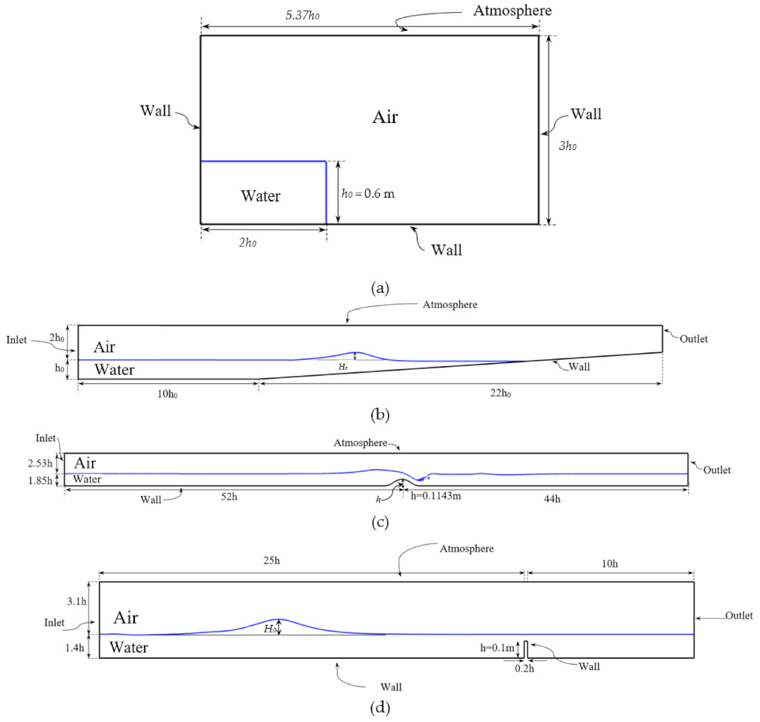
As summarized in Table 1, four sets of simulations were carried out in this study. Figure 1 shows the computational domain and boundary conditions used for the test cases. All the simulations were performed using a 2D domain. 2D domain simulation were performed, as benchmark simulations available in the literature have used 2D simulations, and it has been reported in the literature that 2D simulations replicate most of the flow features predicted by three dimensional simulations [48]. Effect of (RANS) turbulence modeling on the plunging wave breaking characteristics were studied for the solitary wave run-up case (discussed below), which showed that high turbulent eddy viscosity in the air flow deteriorated the breaking predictions. Further, Alberello et al. [48] reported that for 2D simulations wave breaking predictions were not significantly affected by turbulence models. Thus, most of the simulations were performed using laminar flow conditions.
Case #1 involved simulations for dam break without obstacle. This case involved a plunging breaking wave due flow reflection from the bounding wall. The simulations were performed using a computational domain of 3h0 × 5.37h0, where h0 is the initial water column depth of 0.6 m. The water column width was 2h0. The left, right, and bottom walls were specified to be no-slip boundary condition, while atmosphere conditions with zero pressure were specified at the top boundary. Proteus simulations were performed on five 5 systematically refined grids ranging from 28 thousand (K) to 88 K cells. The OpenFOAM simulations were performed using three 3 grid with 44 K, 64 K, and 87 K cells, such that the finest grid was of similar size for both solvers. For this case, the OpenFOAM and Proteus results were compared against each other, and validated against experimental data [49], and benchmark CFD results available in the literature using different multiphase models [15,50,51].
Case #2 involved simulations for solitary wave run-up on 1:15 slope (s). OpenFOAM simulations were performed for five different wave elevations H0/h0 = 0.06, 0.1, 0.3, 0.45, and 0.6. The breaking criterion = 0.41, 0.32, 0.19, 0.15, and 0.13 for H0/h0 = 0.06, 0.1, 0.3, 0.45, and 0.6, respectively. Grilli et al. [6] proposed that the type of wave breaking can be estimated from , as below:
Thus, no-breaking was expected for H0/h0 = 0.06, surging breaking for H0/h0 = 0.1, and plunging breaking for H0/h0 = 0.3, 0.45, and 0.6. Simulations over a range of wave height help assess the predictive capability of CFD methods for a range of wave breaking events spanning from no-breaking, to surging, to plunging breaking. Proteus simulations were performed for a selected plunging breaking case with H0/h0 = 0.45. The simulation domain was composed of two sections: the initial flat bottom section from x/h0 = [−10,0] and z/h0 = [−1,2] which was incorporated to stabilize the solitary wave inflow before the run up, and the slopping bottom section from x/h0 = [0,22.5] and z/h0 = [−1,2]. A no-slip boundary condition was used for the sloping bottom, atmospheric condition for the top surface, and solitary wave inflow was applied at the far-left inlet. The solitary wave was prescribed an initial condition using the Boussinesq wave equation described in Equations (8,9,10,11). Grid study was performed for both OpenFOAM and Proteus for the H0/h0 = 0.45 case. OpenFOAM simulations for other H0/h0 cases were performed using the finest 747 K cell grid. OpenFOAM and Proteus results were compared with each other, along with the potential flow results from [6] and validated using experimental data [2].
Case #3 involved flow over a bump, which resulted in a backward plunging breaking wave downstream of the bump as flow encounters reflection due to hydraulic jump. The flow conditions corresponded to the experimental conditions of [11] and the initial water depth is 1.85 h, where h = 0.1143 m is the bump height, i.e., the water depth over the bump is 0.85 h. Simulations were performed using a computational domain that extended from x/h = [−52,44] and z/h = [0,4.38], where the bump peak is located at the domain origin x,z = [0,h]. A uniform water inflow velocity of 0.87 m/s and air velocity of 0 m/s was used on the left face of the domain, outlet on the right face, atmospheric conditions on the top, and no-slip at the bottom surface. Proteus simulations were performed using multiple grid sizes ranging from 96 K to 972 K cells. OpenFOAM simulations were performed using two 2 grids consisting of 400 K and 1 million (M) cells. The OpenFOAM and Proteus simulations were compared against experimental data [11] and benchmark CFD results from [12].
Case #4 involved flow of solitary wave over a submerged rectangular obstacle with width to height ratio of 0.2. The solitary wave height H0/h0 = 0.5, and the water depth is 1.4 h, where h is the obstacle height. This case involved backward plunging breaking wave due to obstacle induced vortices. Simulations were performed using a rectangular domain with x/h = [–25,10] and z/h = [0,4.5]. The obstacle bottom-left corner was located at the origin of the domain x,z = [0,0]. The height of the barrier is h = 0.1 m and width w = 0.2h. The bottom surface and the obstacle were specified to be no-slip surfaces, and atmospheric condition was applied on the top surface. The solitary wave was prescribed an initial condition using the Boussinesq wave equation described in Equations (8)–(11). For this case only OpenFOAM simulations were performed using two grid resolutions of 838 K and 1.6 M cells. The results were validated against experimental data and CFD results from [8].
The computational cost for each test depends almost linearly with the grid size requirements. Thus, Case #4 is the most computationally extensive followed by Case #2 and 3, and Case #1 is the least expensive. In general, for similar grid size, the Proteus simulations required two times more memory and CPU time compared to OpenFOAM. However, a direct comparison between Proteus and OpenFOAM computational cost does not reflect the computational cost associated with VoF vs CLVoF. The two solvers use very different solution convergence, in particular finite-element Proteus requires much lower convergence tolerance compared to finite-volume OpenFOAM. In addition, the large memory requirement for Proteus is perhaps because the solver is Python based, whereas OpenFOAM is C++ based.
4. Results and Discussion
4.1. Dam Break
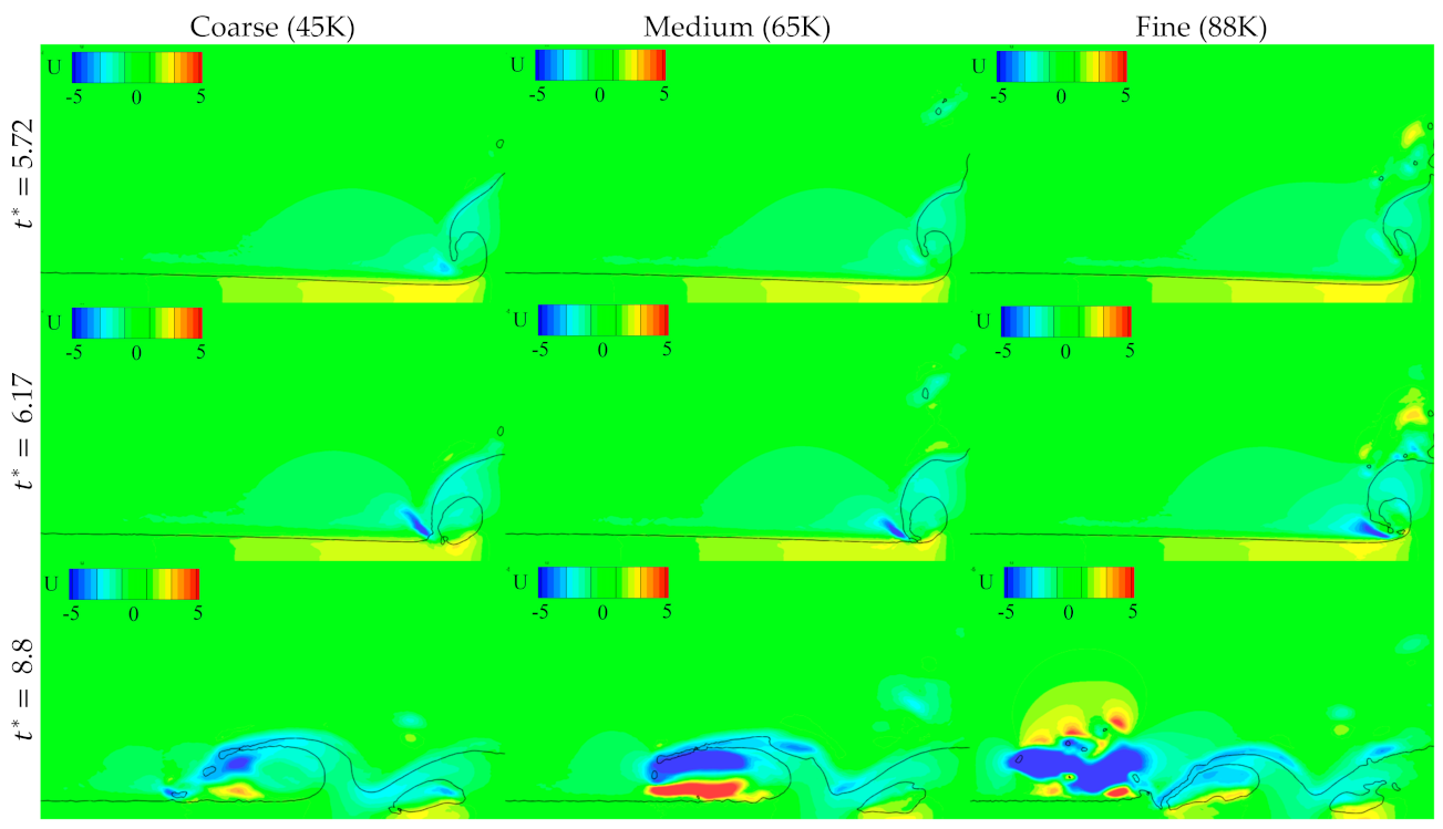
The grid study in Figure 2 shows that the wave elevation predictions qualitatively improved with grid resolution, and fine grid prediction resolved formation of droplets. The plunging breaking was somewhat delayed with grid refinement, and the differences were quite noticeable between the 44 K cells (coarse) and 64 K cells (medium) grids, and less noticeable between the medium and 87 K cells (fine) grids. Further, the plunger shape showed variation with grid refinement. As the grid was refined, the plunger became sharp, but the tips curled up and the breaking was not very sharp. The detailed results on all the different grids have been presented in Hubbard [43] and not shown herein. The results on the fine grid are used for the validation study below.
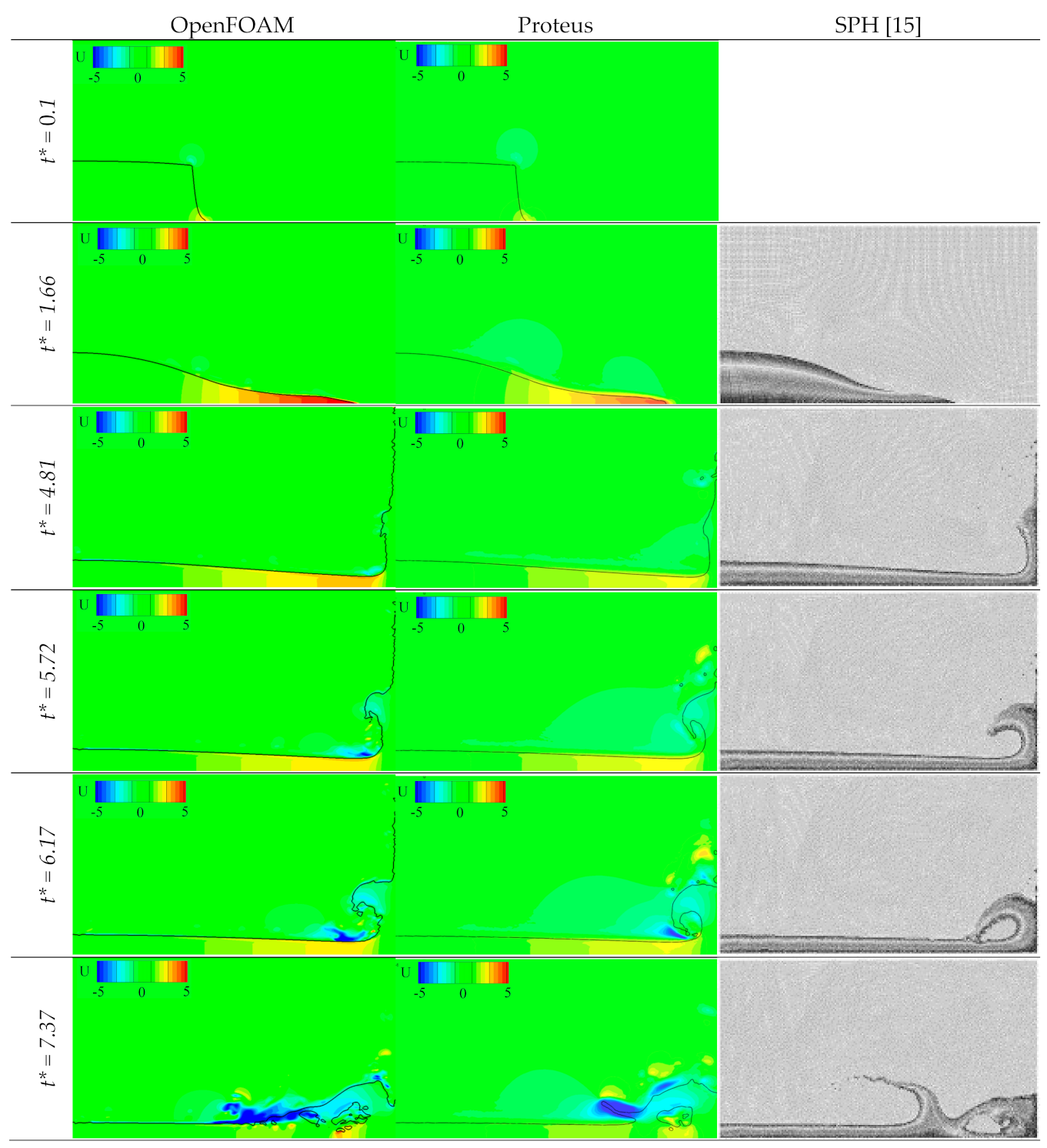
The OpenFOAM and Proteus predictions of the different stages of flow were compared against benchmark CFD data of [15] obtained using smoothed particle hydrodynamics (SPH) in Figure 3. At = 0.1, where h is the initial water depth, the water column starts to move towards the right of the domain due to the gravity force. At t* = 1.66, the water column collapses entirely and the front face of the water moves swiftly towards right of the domain. Both OpenFOAM and Proteus predictions are comparable at this stage. At t* = 4.81, the water collides with the right wall and moves upwards due to its momentum. Proteus predicts much smoother air–water interface than OpenFOAM and shows the formation of water droplets similar to SPH. At t* = 5.72, the water is reflected from the wall and plunger is formed. Both OpenFOAM and Proteus results shows that the plunger is more curled up compared to the SPH results. At t* = 6.17, the plunger predicted by Proteus seems to break on to the water surface, but the plunger is significantly curled compared to SPH results. The OpenFOAM predictions show that the plunger is still forming. At t* = 7.37, a second plunger is formed as the water is reflected from the water surface. Proteus shows a well-defined second plunger, but they are not formed well in OpenFOAM.
In Figure 4, the wave profiles at different stages of breaking at t* = 5.95, 6.20, 6.76, and 7.14 predicted by OpenFOAM (OF) and Proteus (PR) are compared with the boundary element method (BEM) results from [50], SPH results on coarse grid (SPH1), fine grid (SPH2) from [15], and level-set (LS) results reported in [51]. At t* = 5.95, the plunger predicted by BEM and SPH show similar shape and the Proteus result shows more curvature towards the waterbed. OpenFOAM follows Proteus plunger shape, however, the plunger is not well formed. At t* = 6.20, BEM and SPH results show the plunger touches the water surface at x = 4.12. OpenFOAM displays a contact point much closer to the wall at x = 4.5. Proteus follows SPH and BEM pattern, however a second plunger is already formed at x = 4.25. At t* = 6.76, the plunger has crashed onto the water surface and the second plunger is observed for SPH, LS and Proteus at around x = 3.75. Note that BEM results are not available for this stage of the flow. The second plunger is not visible in OpenFOAM results. At t* = 7.14, SPH, LS, and Proteus predictions show that the second plunger is preparing to crash onto the water surface for a second time, while OpenFOAM shows a small water elevation at the location of the second plunger.
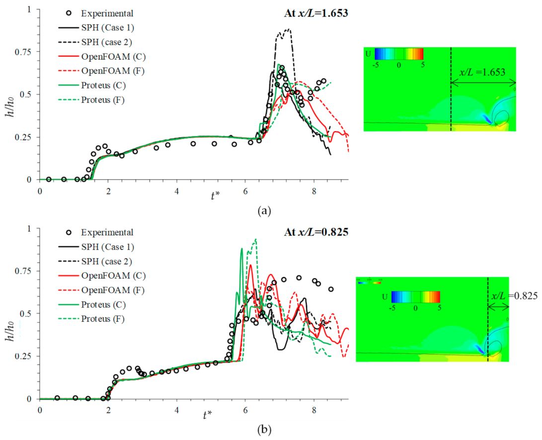
Figure 5 compares the total water height at x/L = 1.653 and 0.825 predicted by Proteus and OpenFOAM with experimental data and SPH results [15], where L = 5.37h0 is the length of the domain. As shown in the figure, the former location is closer to the initial water column than the latter. At x/L = 1.653, the water height is zero up to t* = 1.75 as the water from the dam break has not reached the probe location. The water depth shows a sharp increase after that, and experiments show a peak at t* = 2. The water depth increases sharply around t* = 6.4 as the water reflected from the back wall reaches the probe location. All the simulations, including the benchmark CFD results, fail to predict the peak at t* = 2, this suggests that fluid velocity is somewhat overpredicted in the simulations. All the simulations predict the increase in water depth at t* = 6.4 very well. The peak water depth at t* = 7.2 is predicted best by SPH on fine grid and Proteus on coarse grid. However, for t* > 7.2, the simulations show a sharp decrease in the water depth, except for those predicted by Proteus on the fine grid.
At x/L = 0.825, the water depth starts to increase at t* = 2 when the water from the dam break reaches the probe location. The second increase starts at t* = 5.4, when the water reflected from the wall reaches the probe location. Similar to the predictions at x/L = 1.653, none of the simulations predict the water depth peak at t* = 2. The second increase in water depth is predicted well by SPH simulations and Proteus simulations on coarse grid. OpenFOAM results on both coarse and fine grids and Proteus results on fine grid show a delay in the water depth increase, due to delay in the breaking. For t* > 6.8, simulations do not predict the higher water depth observed in the experiment.
4.2. Solitary Wave Run-Up over a Slope
A detailed grid study was performed using both OpenFOAM and Proteus for H0 /h0 = 0.45 case to identify appropriate grid resolution for the simulations. OpenFOAM simulations were also performed using RANS turbulence model to understand the effect of turbulence on the predictions. Readers are referred to Chambers [42] and Hubbard [43] for details. Salient points of the study are presented here.
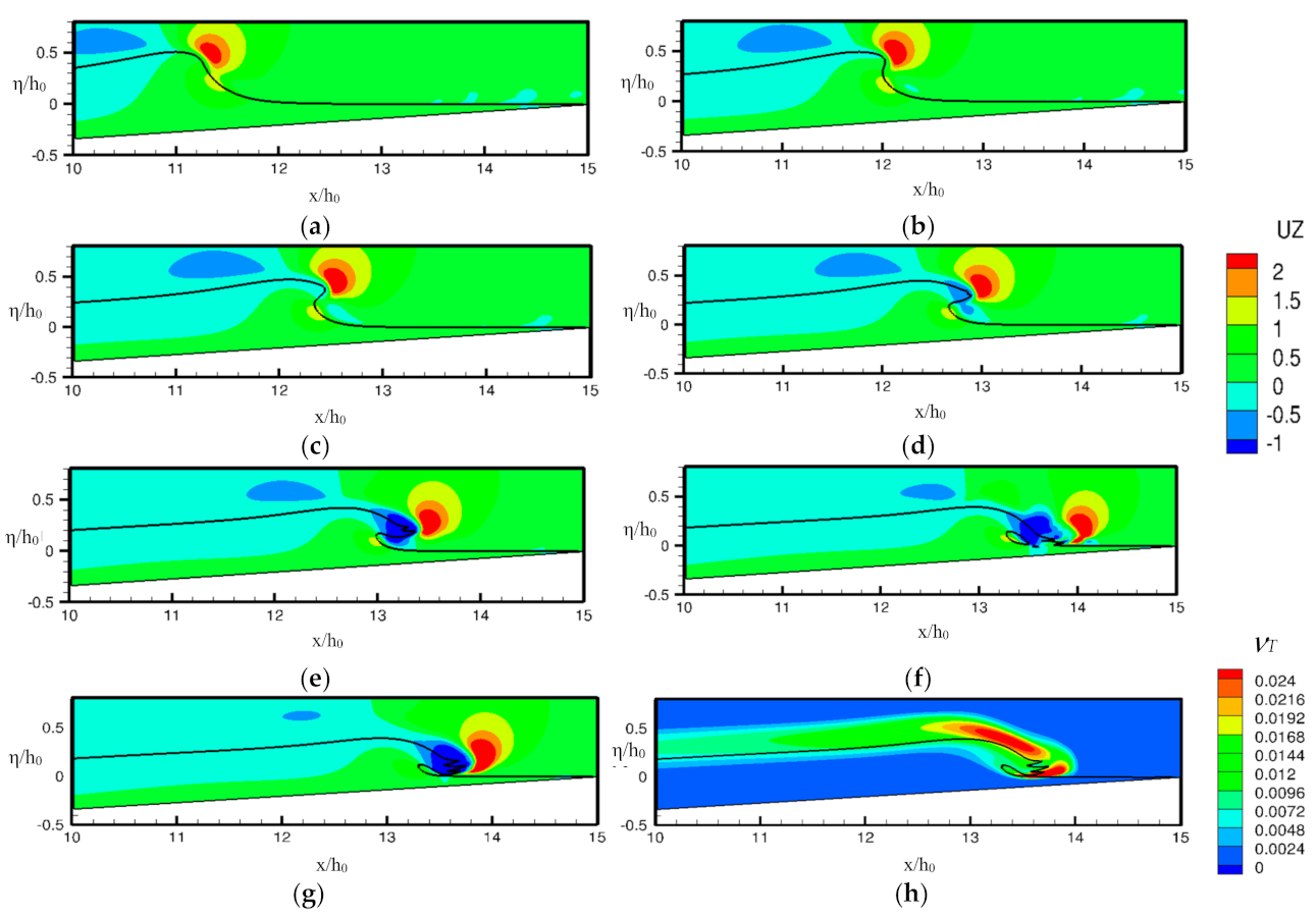
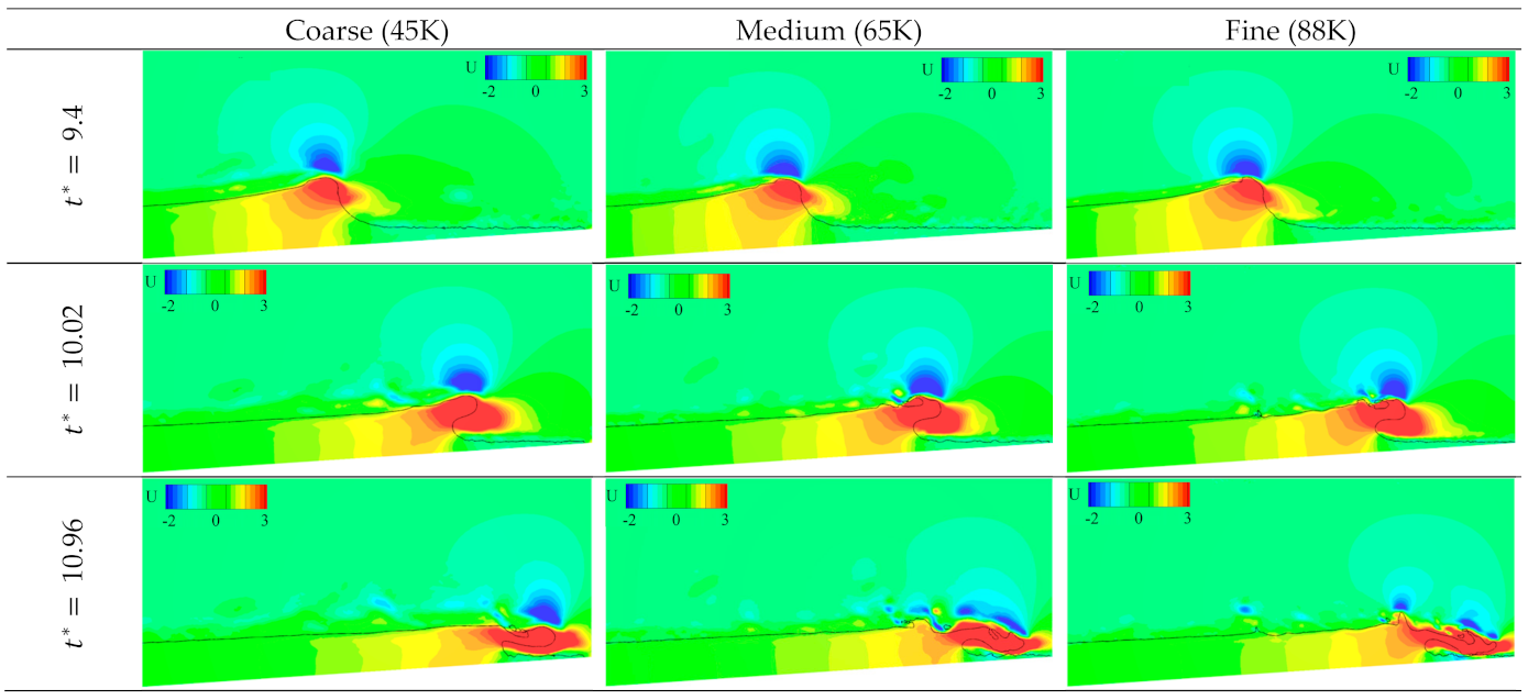
The evolution of the solitary wave for the H0 /h0 = 0.45 case as it moves over the slope is shown in Figure 6a–f. It can be observed that by = 9.4 the wave front starts to curve forward. By = 9.7 to 10 a plunger is formed which breaks forward by = 10.96. The interaction between the plunger and the water surface results in the formation of a small air cavity trapped at x = 13.5h0. The vertical velocity contours show the presence of high air velocity which pushes the plunger tip upwards, whereas the water velocity in the plunger moves it downwards. The OpenFOAM grid refinement study revealed that the free-surface resolution, in particular the plunger shape, improved with the grid refinement from 146 K (coarse) to 396 K (medium) grid, but no significant improvement was obtained on further grid refinement to 747 K (fine) cells. The Proteus predictions in Figure 7 showed significant changes on the grid resolution, in particular the free-surface was not smooth on the finer grids and surface peel-off (due to air flow opposite to water flow) increased with refinement. Considering a tradeoff between accuracy and computational cost, the medium grid is used for the validation study below.
The OpenFOAM RANS simulations (predictions at = 10.96 shown in Figure 6g) showed somewhat lower peak wave height and the plunger reconnection was delayed compared to the laminar case, and the plunger tip shows a zagged shape. To investigate this effect, the turbulent eddy viscosity predictions were analyzed. The results at = 10.96 (shown in Figure 6h) showed presence of high turbulent eddy viscosity (νT) in the air flow especially in the plunging flow and in the reconnection region, where the peak νT ~ 1.5 × 10⁴ν. The lower wave height is probably due to excessive fluid momentum decay by turbulent eddy viscosity, and the zagged plunger is probably due to augmentation of the air flow.
OpenFOAM simulations were also performed for two low wave heights H0 /h0 = 0.06 and 0.1. The wave elevation predictions for these cases are compared with Potential flow results [6] in Figure 8. For both the cases the OpenFOAM predictions compared very well with potential flow results. As expected, the H0/h0 = 0.06 case does not show any breaking as the base of the wave moves faster than the surface. The H0/h0 = 0.06 case shows a surging breaking behavior. The wave forms a crest, but a plunger is not formed. The wave crest rises vertically and collapses.
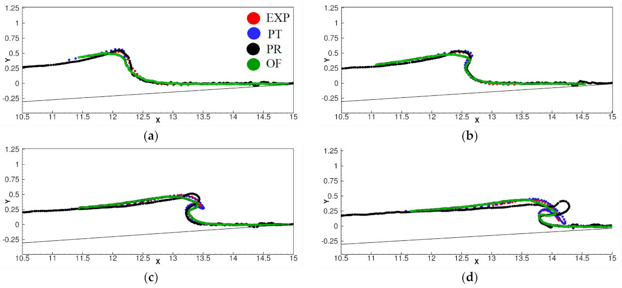
Proteus and OpenFOAM instantaneous wave elevation predictions for H0/h0 = 0.45 are compared against the experimental measurements from [2] and the potential flow results from [6] in Figure 9. Figure 9a,b shows the plunger formation, Proteus predictions at this stage compare very well with the experimental data and the potential flow results, whereas OpenFOAM somewhat underpredicts the peak wave height. In Figure 9c experimental data and the Potential flow results show the formation of thin and sharp plunger curving towards the waterbed. OpenFOAM fails to predict the thin edge of the plunger and Proteus displays a blunt plunger facing upwards. In Figure 9d experimental data and the Potential flow results show the breaking of the plunger onto the water surface. OpenFOAM results show that the plunger crash is delayed, whereas Proteus does not predict a sharp plunging pattern.
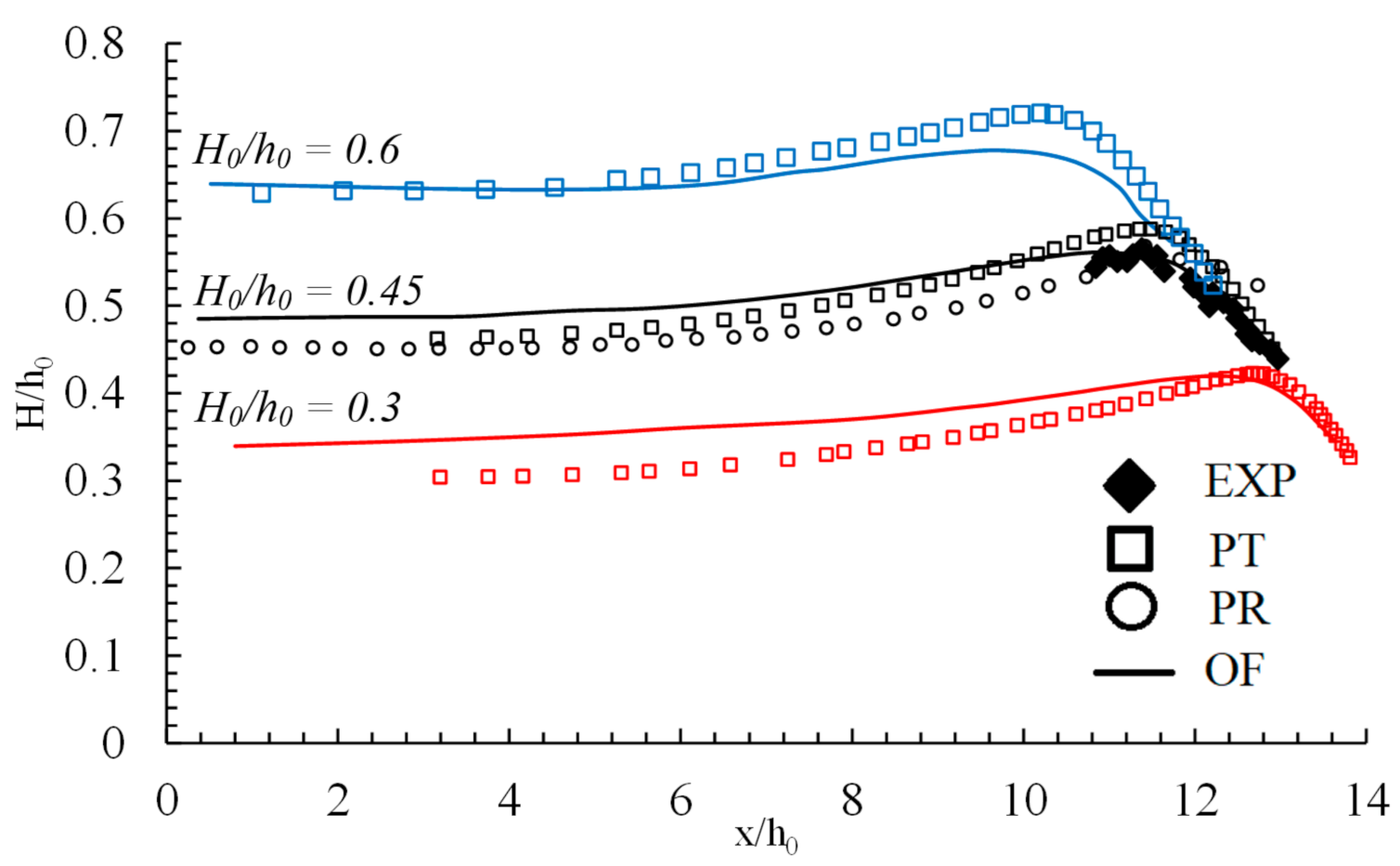
Figure 10 compares the peak wave height along the slope location predicted by OpenFOAM and Proteus for plunging breaking cases H0/h0 = 0.3, 0.45, and 0.6 with experimental data and Potential flow results. Note that Proteus results were obtained for H0/h0 = 0.45 only. Results show that the peak wave height occurs earlier as H0/h0 increases. The peak wave height corresponds to the instance when the plunger starts to form and move downwards. Thus, the breaking also occurs earlier with the increase in H0/h0. For H0/h0 = 0.3, the peak wave height is observed at x/h0 = 13, OpenFOAM overpredicts the wave height up until the peak location, but the predictions agree well with Potential flow after the wave plunges downward. For H0/h0 = 0.6, OpenFOAM underpredicts the peak wave height at x/h0 = 11. For H0/h0 = 0.45, both OpenFOAM and Proteus predict the correct plunging behavior, while the Potential flow overpredicts the peak wave height.
4.3. Flow over a Submerged Bump
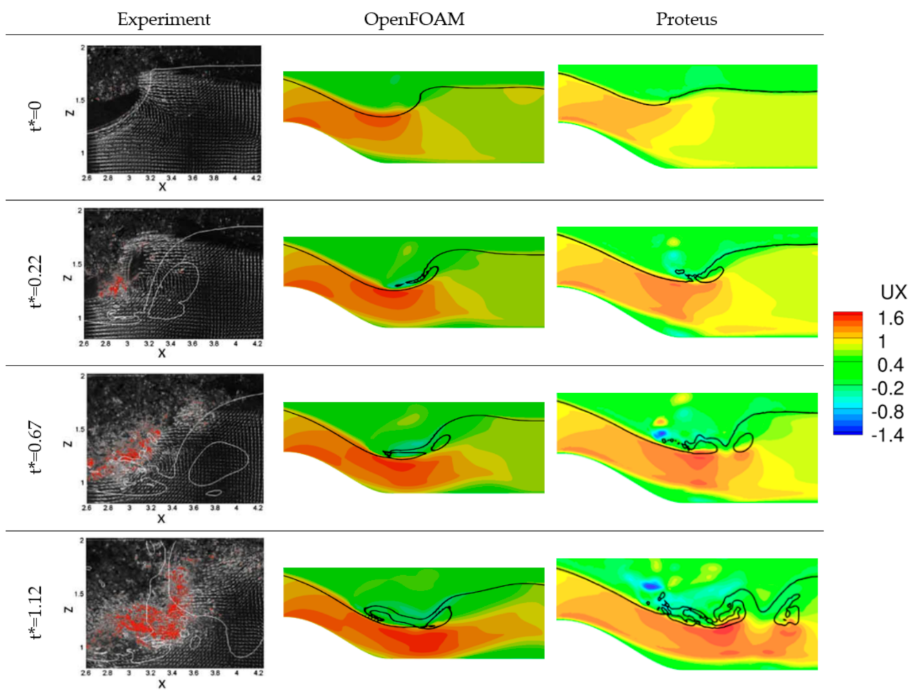
The free surface is flat prior to the bump, and the wave plunging is initiated by the presence of the submerged bump. As depicted in Figure 11, this case shows a series of wave breaking processes: high wave crest, first plunger, splash up, vertical jet, repeated plunger with moderate splash ups and vertical jet, and finally chaotic motions. The time is adjusted such that t* (t h/U) = 0 corresponds to the stage when the step wave crest is formed, and the backward plunger is at the verge of formation.
At t* = 0, OpenFOAM underpredicts the sharpness of the wave crest compared to the experiment, while Proteus fails to predict the crest well. At t* = 0.22, experiments show a sharp backward plunge. OpenFOAM predictions show an overturning jet which is about to interact with the water surface, However, the plunge is not that sharp and curved away from the surface. Proteus predicts a reconnection between the plunger and the water surface similar to the experiment, but the trapped water bubble is more elongated than in the experiment. At t* = 0.67, the experiment shows a splash up and formation of second plunger towards the left of the domain. OpenFOAM predicts a moderate splash up, while Proteus predicts the oblique splash up much better. At t* = 1.22, the experimental data shows a chaotic behavior and presence of a high vertical jet. OpenFOAM predicts less intense overturning jet compared to Proteus, and the latter seems to capture the presence of a second plunger and the vertical jet well.
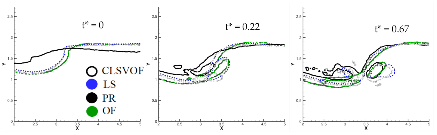
Figure 12 compares the water elevation profiles predicted by OpenFOAM and Proteus with the CLSVoF and LS predictions reported by [12] at three different stages of breaking. The benchmark CFD results from [12] do not show significant differences between the CLSVOF and LS predictions, except that the former captures the trapped air bubbles better than LS. At t* = 0, OpenFOAM predictions compare very well with the benchmark results, whereas Proteus fails to predict the vertical wave crest. At t* = 0.22, benchmark results show a sharp thin plunger breaking onto the water surface along with an air cavitation zone at x = 3.25h. Both OpenFOAM and Proteus predict the plunger breaking location at around x = 3h, and the trapped air bubble is more horizontally elongated. At t* = 0.67, as the wave crashes onto the water surface a splash up is observed. Proteus shows a good agreement with benchmark CFD results, while OpenFOAM predicts a moderate splash up.
4.4. Solitary Wave over a Submerged Rectangular Obstacle
For this case, the flow pattern upstream of the obstacle shows advection of the solitary wave, but the flow downstream of the obstacle involves interesting features associating breaking waves and vortex shedding. Thus, the analysis of the results focuses only on the section downstream of the obstacles in Figure 13 and Figure 14.
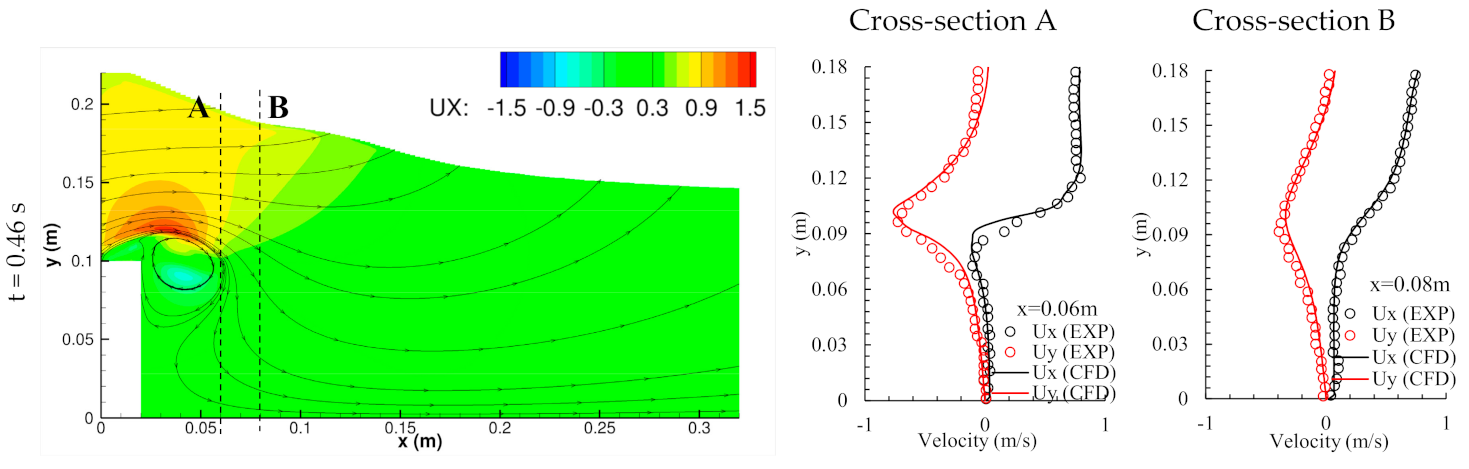
The experimental data [8] provides free surface elevation, velocity streamlines (or vectors) and vorticity contours at five intervals t = 0.46 s, 0.6 s, 0.74 s, 0.88 s, and 1.02 s. At t = 0.46 s, the incoming wave approaches the obstacle and a bulge grows at the water surface near the leeward side of the obstacle at x = 0.1 m. This bulge grows away from the obstacle to form a new wave crest at x = 0.23 m around t = 0.6 s. At this stage the initial incoming solitary wave crest has gradually decayed, and the solitary wave flow (mass) has been transferred to the new wave crest. This phenomenon is called crest–crest exchange [52]. At t = 0.74 s, the wave has entirely traveled over the obstacle, and the leeward side of the wave shows a steep slope. The steep slope continues to grow at t = 0.88 s and a plunger is about to form. At t = 1.02 s, a backward wave breaking is observed which is accompanied by water splash up, and the overturning jet entraps air bubbles into the water at x = 0.15 m.
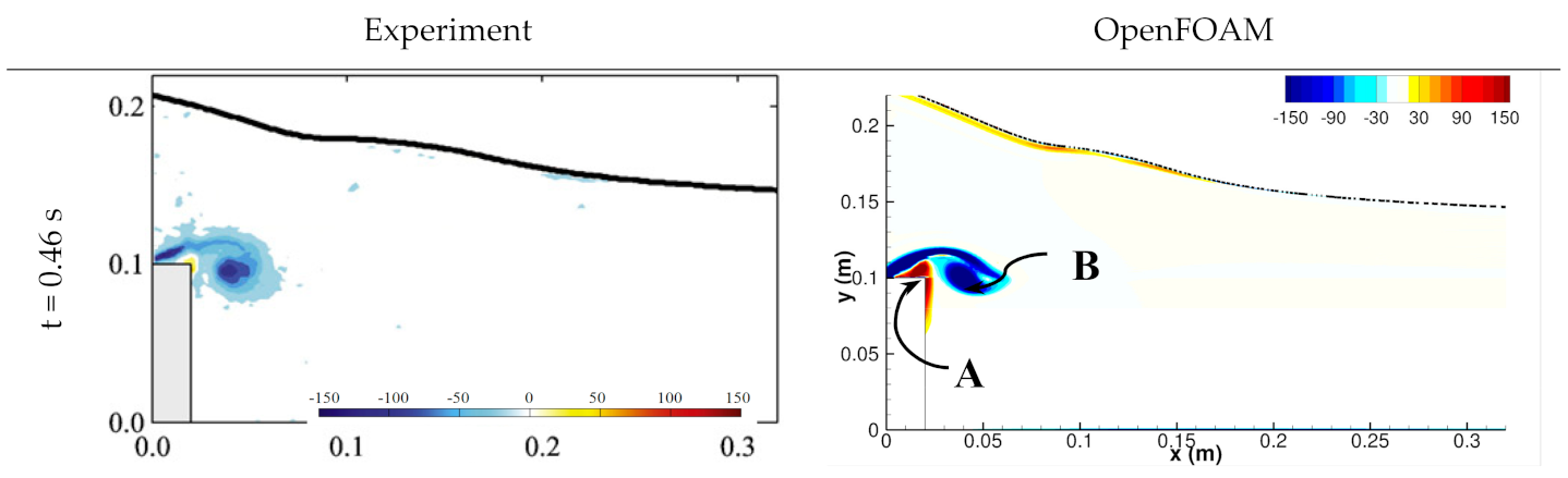
The vorticity contours in Figure 14 primarily show a vortex sheet emerging from the leading edge of the obstacle, which is shed and advected downstream. A secondary counter-rotating vortex is formed from the air–water interface at t = 0.88 s and shed downstream.
OpenFOAM predicts the four phases of the flow: wave transmission, crest to crest exchange, backward wave breaking, and secondary splash up consistent with the experimental data. One of the primary differences between the CFD prediction and experiment is the formation of the entrapped air-bubble at t = 1.02 s. The CFD predictions reported by [8] also showed a similar air bubble. The formation of the backward plunging jet and splash-up events are predicted better on finer grid than those on the coarse grid. The primary vortex shedding predicted by CFD compares very well with the experimental data. CFD provides a detailed description of the vortex shedding pattern compared to the experiment. At t = 0.46 s, a vortex sheet is formed from the obstacle leading edge followed by a counter-rotating vortex bubble on the top of the obstacle (marked as vortex A). The latter pushes the former away from the obstacle resulting in the vortex shedding (marked as vortex B). The CFD also predicts the formation of the secondary counter-rotating vortex from the air–water interface at t = 0.88 s, which is shed at t = 1.02 s. CFD predicts an additional counter-rotating vortex during the splash event (marked at vortex C), which is not predicted in the experiment. The CFD predictions also provide a detailed description of the interaction of the primary vortex with the bottom surface resulting in counter-rotating vortices.
The horizontal and vertical velocity profiles along cross-sections passing through the vortex core, and slightly downstream or upstream, are compared with experimental data in Figure 13 The predicted profiles show good agreement with the experimental data at the pre-wave breaking stages. Some discrepancies are observed post-breaking t = 0.88 s and 1.02 s for z > 0.06 m, in particular the streamwise and normal velocities are overpredicted.
A synthesis of the experimental and CFD results provides insight into the cause of the backward plunging breaking. The primary vortex shed from the obstacle caused the flow to stagnate downstream of the obstacle accelerating the flow in the narrow region above the vortex and below the free surface. This highly accelerating flow underwent a hydraulic jump behavior transferring mass from solitary wave to the secondary crest (crest–crest exchange). The accelerating flow in return induced a counter-rotating vortex underneath the free-surface overturning the flow backward, resulting in the plunging breaking pattern.
5. Conclusions
The study evaluates the capability of Navier–Stokes solvers in predicting forward and backward plunging breaking caused by either flow acceleration (such as over a slope or a submerged hump) or flow reflection from the wall or submerged obstacle induced vortices, including assessment of the effect of grid resolution and turbulence modeling on the predictions and comparison of VoF and CLSVoF air–water interface modeling methods. To achieve the objective, simulations have been performed using OpenFOAM, a finite-volume solver with the VoF method, and Proteus, a finite-element solver with a CLSVoF method. Four test cases were considered: dam break—which involves backward plunging breaking due to flow reflection from the wall; run-up of solitary waves over a slope—resulting in either no-breaking or surging or forward plunging breaking; uniform flow over a submerged bump—resulting in backward plunging breaking due to blockage of the downstream flow because of hydraulic jump; and solitary wave flow over a submerged obstacle—resulting in backward plunging breaking due to flow circulation induced by vortices shed from the obstacle.
The grid study shows that grid refinement helps improve the resolution of the air–water interface, particularly in the breaking and splash regimes; however, after a certain limit grid refinement does not improve the prediction of physical features. In fact, on very fine grids, instabilities were triggered at the air–water interface (primarily for the air flow) which induced surface peel-off or kinks and roll-up of the plunger tips.
The effect of the turbulence model was evaluated for the prediction of plunging breaking for solitary wave run-up over a slope. The RANS turbulence models predicted high eddy-viscosity in for the air flow, which decayed the fluid momentum and resulted in lower peak wave height during the run-up. High eddy viscosity was also predicted in the air-region close to the reconnection, which adversely affected the plunger shape. The laminar flow results were found to be both qualitatively and quantitatively better than the RANS results, thus most of the simulations were performed using laminar flow conditions.
Overall, both the finite-element CLSVoF and finite-volume VoF solvers predicted the large-scale plunging breaking characteristics, such as generation of the steep wave slope, plunger formation and breaking well; however, they varied in the prediction of the finer details. The CLSVoF solver predicts the splash-up event and secondary plunger better than the VoF solver; however, the latter predicts the plunger shape better than the former for the solitary wave run-up on a slope case. The CLSVoF solver also shows surface peel-off due to the generation of air flow in the direction opposite to the water flow. For the solitary wave flow over a submerged obstacle, CFD predictions reveal that the vortex generated underneath the free surface causes the backward plunging breaking wave. The free-surface vortex is formed due to flow acceleration in the narrow region above the obstacle and free-surface due to flow stagnation behind the obstacle.
Future work will focus on extending the simulation to 3D flows. Alberello et al. [48] reported that turbulence modeling becomes important for 3D simulations, and three-dimensional flow structures start to appear in the breaking region.
Author Contributions
Conceptualization, S.B., O.E.F. and C.K.; methodology, S.B.; software, B.C., G.H., C.K. and O.E.F.; validation, B.C., G.H., O.E.F. and S.B.; formal analysis, S.B.; investigation, S.B., B.C. and O.E.F.; resources, S.B., C.K.; data curation, S.B., B.C., G.H. and O.E.F.; writing—original draft preparation, S.B. and O.E.F.; writing—review and editing, S.B., O.E.F., and C.K.; visualization, S.B. and O.E.F.; supervision, S.B. and C.K.; project administration, S.B., C.K.; funding acquisition, S.B. and C.K. All authors have read and agreed to the published version of the manuscript.
Funding
Effort at Mississippi State University was sponsored by the Engineering Research & Development Center under Cooperative Agreement number W912HZ-17-2-0014. The views and conclusions contained herein are those of the authors and should not be interpreted as necessarily representing the official policies or endorsements, either expressed or implied, of the Engineering Research & Development Center or the U.S. Government.
Institutional Review Board Statement
Not applicable.
Informed Consent Statement
Not applicable.
Data Availability Statement
Data presented in the study can be obtained from authors upon request Email: [email protected].
Conflicts of Interest
The authors declare no conflict of interest.
References
- Helfrich, K.R. Internal solitary wave breaking and run-up on a uniform slope. J. Fluid Mech. 1992, 243, 133–154. [Google Scholar] [CrossRef]
- Li, Y.; Raichlen, F. Non-breaking and breaking solitary wave run-up. J. Fluid Mech. 2002, 456, 295–318. [Google Scholar] [CrossRef] [Green Version]
- Chou, C.; Ouyang, K. Breaking of Solitary Waves on Uniform Slopes. China Ocean Eng. J. 1999, 4, 429–442. [Google Scholar]
- Grilli, S.T.; Svendsen, I.A.; Subramanya, R. Breaking Criterion and Characteristics for Solitary Waves on Slopes. J. Waterw. Port, Coast. Ocean Eng. 1997, 123, 102–112. [Google Scholar] [CrossRef] [Green Version]
- U.S. Department of Transportation Federal Highway Administration. Available online: https://www.fhwa.dot.gov/engineering/hydraulics/pubs/09111/09112.pdf (accessed on 18 September 2020).
- Grilli, S.T.; Losada, M.Á.; Martin, F. Characteristics of Solitary Wave Breaking Induced by Breakwaters. J. Waterw. Port, Coast. Ocean Eng. 1994, 120, 74–92. [Google Scholar] [CrossRef] [Green Version]
- Wu, Y.-T. Numerical Investigation of Solitary Wave Interaction with a Submerged Vertical Thin Barrier. Master’s Thesis, National Cheng Kung University, Cheng Kung, Taiwan, 2010. [Google Scholar]
- Wu, Y.-T.; Hsiao, S.-C.; Huang, Z.-C.; Hwang, K.-S. Propagation of solitary waves over a bottom-mounted barrier. Coast. Eng. 2012, 62, 31–47. [Google Scholar] [CrossRef]
- Wang, J.; He, G.; You, R.; Liu, P. Numerical study on interaction of a solitary wave with the submerged obstacle. Ocean Eng. 2018, 158, 1–14. [Google Scholar] [CrossRef]
- Wang, Y.; Wang, G.; Li, G. Experimental study on the performance of the multiple-layer breakwater. Ocean Eng. 2006, 33, 1829–1839. [Google Scholar] [CrossRef]
- Ghosh, S. Free Surface Instabilities and Plunging Breaking Waves Downstream of a Bump in a Shallow Water Open Channel Flume. Ph.D. Thesis, The University of Iowa, Iowa City, IA, USA, 2008. [Google Scholar]
- Wang, Z.; Yang, J.; Koo, B.; Stern, F. A coupled level set and volume-of-fluid method for sharp interface simulation of plunging breaking waves. Int. J. Multiph. Flow 2009, 35, 227–246. [Google Scholar] [CrossRef]
- Stansby, P.K.; Chegini, A.; Barnes, T.C.D. The initial stages of dam-break flow. J. Fluid Mech. 1998, 374, 407–424. [Google Scholar] [CrossRef]
- Kamra, M.M.; Mohd, N.; Liu, C.; Sueyoshi, M.; Hu, C. Numerical and experimental investigation of three-dimensionality in the dam-break flow against a vertical wall. J. Hydrodyn. 2018, 30, 682–693. [Google Scholar] [CrossRef]
- Colagrossi, A.; Landrini, M. Numerical simulation of interfacial flows by smoothed particle hydrodynamics. J. Comput. Phys. 2003, 191, 448–475. [Google Scholar] [CrossRef]
- Alberello, A.; Iafrati, A. The Velocity Field underneath a Breaking Rogue Wave: Laboratory Experiments versus Numerical Simulations. Fluids 2019, 4, 68. [Google Scholar] [CrossRef] [Green Version]
- Wackers, J.; Koren, B.; Raven, H.C.; Van Der Ploeg, A.; Starke, A.R.; Deng, G.B.; Queutey, P.; Visonneau, M.; Hino, T.; Ohashi, K. Free-Surface Viscous Flow Solution Methods for Ship Hydrodynamics. Arch. Comput. Methods Eng. 2011, 18, 1–41. [Google Scholar] [CrossRef] [Green Version]
- Oger, G.; Rousset, J.M.; Le Touze, D.; Alessandrini, B.; Fxerrant, P. SPH simulations of 3-D slamming problems. In Proceedings of the 9th International Conference on Numerical Ship Hydrodynamics, Washington, DC, USA, 5–8 August 2007. [Google Scholar]
- Shibata, K.; Koshizuka, S.; Tanizawa, K. Three-dimensional numerical analysis of shipping water onto a moving ship using a particle method. J. Mar. Sci. Technol. 2009, 14, 214–227. [Google Scholar] [CrossRef]
- Hirata, N.; Hino, T. An Efficient Algorithm for Simulating Free-Surface Turbulent Flows around an Advancing Ship. J. Soc. Nav. Arch. Jpn. 1999, 1999, 1–8. [Google Scholar] [CrossRef] [Green Version]
- Starke, B.; van der Ploeg, A.; Raven, H. Viscous free surface flow computations for self-propulsion conditions using PARNASSOS. In Proceedings of the Gothenburg 2010: A Workshop on CFD in Ship Hydrodynamics, Gothenburg, Sweden, 7 December 2010. [Google Scholar]
- Alessandrini, B.; Delhommeau, G. A Fully Coupled Navier-Stokes Solver for Calculations of Turbulent Incompressible Free Surface Flow Past A Ship Hull. Int. J. Numer. Methods Fluid 1999, 29, 125–142. [Google Scholar] [CrossRef]
- Li, T.; Matusiak, J. Simulation of a modern surface ship with a wetted transom in a viscous flow. In Proceedings of the 11th International Offshore and Polar Engineering Conference, Stavanger, Norway, 17–22 June 2001. [Google Scholar]
- Sussman, M.; Fatemi, E.; Osher, S.; Smereka, P. A level set approach for computing solutions to incompressible two- phase flow II. In Proceedings of the Sixth International Symposium on Computational Fluid Dynamics, Lake Tahoe, NV, USA, 4–8 September 1995. [Google Scholar]
- Hino, T.; Ohashi, K.; Kobayashi, H. Flow Simulations Using Navier-Stokes Solver Surf. In Proceedings of the Gothenburg 2010: A Workshop on CFD in Ship Hydrodynamics, G2010 Workshop. Gothenburg, Sweden, 7 December 2010. [Google Scholar]
- Carrica, P.M.; Wilson, R.V.; Noack, R.; Xing, T.; Kandasamy, M.; Stern, F. A dynamic overset, single-phase level set approach for viscous ship flows and large amplitude motions and maneuvering. In Proceedings of the 26th symposium on Naval Hydrodynamics, Rome, Italy, 26–31 August 2006. [Google Scholar]
- Iafrati, A.; Di Mascio, A.; Campana, E.F. A level set technique applied to unsteady free surface flows. Int. J. Numer. Methods Fluids 2001, 35, 281–297. [Google Scholar] [CrossRef]
- Kim, H.; Yang, C.; Kim, H.J.; Chun, H.H. A Combined Local and Global Hull Form Modification Approach for Hydrodynamic Optimization. In Proceedings of the 28th Symposium on Naval Hydrodynamics, Pasadena, CA, USA, 12–17 September 2010. [Google Scholar]
- Queutey, P.; Visonneau, M. An interface capturing method for free-surface hydrodynamic flows. Comput. Fluids 2007, 36, 1481–1510. [Google Scholar] [CrossRef]
- Manzke, M.; Rung, T. Resistance Prediction and Sea Keeping Analysis with FreSCo+. In Proceedings of the Gothenburg 2010: A Workshop on CFD in Ship Hydrodynamics, G2010 Workshop. Gothenburg, Sweden, 7 December 2010. [Google Scholar]
- Bhushan, S.; Yoon, H.; Stern, F.; Guilmineau, E.; Visonneau, M.; Toxopeus, S.; Simonsen, C.; Aram, S.; Kim, S.-E.; Grigoropoulos, G. Assessment of CFD for Surface Combatant 5415 at Straight Ahead and Static Drift. J. Fluids Eng. 2019, 141, 051101. [Google Scholar] [CrossRef]
- Iafrati, A.; Babanin, A.; Onorato, M. Modulational Instability, Wave Breaking, and Formation of Large-Scale Dipoles in the Atmosphere. Phys. Rev. Lett. 2013, 110, 184504. [Google Scholar] [CrossRef] [PubMed] [Green Version]
- Cointe, R.; Tulin, M.P. A theory of steady breakers. J. Fluid Mech. 1994, 276, 1–20. [Google Scholar] [CrossRef]
- Rhee, S.H.; Stern, F. RANS Model for Spilling Breaking Waves. J. Fluids Eng. 2002, 124, 424–432. [Google Scholar] [CrossRef]
- Muscari, R.; Di Mascio, A. Numerical modeling of breaking waves generated by a ship’s hull. J. Mar. Sci. Technol. 2004, 9, 158–170. [Google Scholar] [CrossRef]
- Düz, B.; Scharnke, J.; Hallmann, R.; Tukker, J.; Khurana, S.; Blanchard, K. Comparison of the CFD Results to PIV Measurements in Kinematics of Spilling and Plunging Breakers. In Proceedings of the Volume 6B: Ocean Engineering, New York, NY, USA, 3–7 August 2020. [Google Scholar]
- Aggarwal, A.; Chella, M.A.; Bihs, H.; Myrhaug, D. Properties of breaking irregular waves over slopes. Ocean Eng. 2020, 216, 108098. [Google Scholar] [CrossRef]
- Muk, S.; Ong, M.C.; Obhrai, C.; Gatin, I.; Vukčević, V. Influences of free surface jump conditions and different k−ω SST turbulence models on breaking wave modelling. Ocean Eng. 2020, 217, 107746. [Google Scholar] [CrossRef]
- Yu, C.; Sheu, T.W. Development of a coupled level set and immersed boundary method for predicting dam break flows. Comput. Phys. Commun. 2017, 221, 1–18. [Google Scholar] [CrossRef]
- Jasak, H.; Jemcov, A.; Tukovic, Z. Openfoam: A C++ library for complex physics simulations. In Proceedings of the International Workshop on Coupled Methods in Numerical Dynamics, Dubrovnik, Croatia, 19–21 September 2007. [Google Scholar]
- Kees, C.E.; Akkerman, I.; Farthing, M.W.; Bazilevs, Y. A conservative level set method suitable for variable-order approximations and unstructured meshes. J. Comput. Phys. 2011, 230, 4536–4558. [Google Scholar] [CrossRef]
- Chambers, B. Numerical Simulations of Breaking Waves and Vehicle Fording Using OpenFOAM. Master’s Thesis, Mississippi State University, Starkville, MI, USA, 2017. [Google Scholar]
- Hubbard, G. Validation of Finite Element Couple Level-Set Volume of Fluid Method for Plunging Breaking Wave Prediction. Master’s Thesis, Mississippi State University, Starkville, MI, USA, 2020. [Google Scholar]
- Hirt, C.; Nichols, B. Volume of fluid (VOF) method for the dynamics of free boundaries. J. Comput. Phys. 1981, 39, 201–225. [Google Scholar] [CrossRef]
- Robertson, E.; Choudhury, V.; Bhushan, S.; Walters, D. Validation of OpenFOAM numerical methods and turbulence models for incompressible bluff body flows. Comput. Fluids 2015, 123, 122–145. [Google Scholar] [CrossRef]
- Bazilevs, Y.; Calo, V.; Cottrell, J.; Hughes, T.; Reali, A.; Scovazzi, G. Variational multiscale residual-based turbulence modeling for large eddy simulation of incompressible flows. Comput. Methods Appl. Mech. Eng. 2007, 197, 173–201. [Google Scholar] [CrossRef]
- Boussinesq, J. Théorie de l’intumescence liquide, applelée onde solitaire ou de translation, se propageant dans un canal rectangulaire. Comptes Rendus l’Académie Sci. 1871, 72, 755–759. [Google Scholar]
- Alberello, A.; Pakodzi, C.; Nelli, F.; Bitner-Gregersen, E.M.; Toffoli, A. Three Dimensional Velocity Field underneath a Breaking Rogue Wave. In Proceedings of the Volume 1: Offshore Technology, Stavanger, Norway, 30 November–1 December 2017. [Google Scholar]
- Zhou, Z.Q.; De Kat, J.O.; Buchner, B. A nonlinear 3-D approach to simulate green water dynamics on deck. In Proceedings of the Seventh International Conference on Numerical Ship Hydrodynamics, Nantes, France, 19–22 July 1999. [Google Scholar]
- Greco, M.; Landrini, M.; Faltinsen, O. Impact flows and loads on ship-deck structures. J. Fluids Struct. 2004, 19, 251–275. [Google Scholar] [CrossRef]
- Colicchio, G.; Landrini, M.; Chaplin, J.C. Level-set modelling of the air-water flow generated by a surface piercing body. In Proceedings of the 8th International Conference on Numerical Ship Hydrodynamics, Busan, Korea, 5–8 August 2003. [Google Scholar]
- Cooker, M.J.; Peregrine, D.H.; Vidal, C.; Dold, J.W. The interaction between a solitary wave and a submerged semicircular cylinder. J. Fluid Mech. 1990, 215, 1–22. [Google Scholar] [CrossRef] [Green Version]
Figure 1.
Simulation domain and boundary conditions for: (a) dam break, (b) solitary wave run-up on a 1:15 slope, (c) flow over a submerged bump, and (d) solitary wave over a submerged obstacle test cases.
Figure 1.
Simulation domain and boundary conditions for: (a) dam break, (b) solitary wave run-up on a 1:15 slope, (c) flow over a submerged bump, and (d) solitary wave over a submerged obstacle test cases.

Figure 2.
Development of water breaking stages predicted by Proteus on coarse, medium, and fine grids. The black line represents the air–water interface, and the contour colors represent the streamwise (horizontal) velocity. Results are shown for three non-dimensional simulation times = 5.72, 6.17 and 8.8.

Figure 3.
Predictions at different stage of the wave breaking for the dam break case. Results from OpenFOAM (left column), Proteus (middle) and SPH from Colagrossi and Landrini [15] (right column) at non-dimensional simulation time = 0.1, 1.66, 4.81, 5.72, 6.17 and 7.37 are compared. The black line represents the air–water interface, and the contour colors in the OpenFOAM and Proteus results show the streamwise (horizontal) velocity. SPH plots have been reprinted from Journal of Computational Physics, 191, Andrea Colagrossi and Maurizio Landrini, Numerical simulation of interfacial flows by smoothed particle hydrodynamics, pp. 448–475, Copyright (2021), with permission from Elsevier.

Figure 4.
Wave profiles at different breaking stages = 5.95, 6.20, 6.76. and 7.14. Boundary element method (BEM) results [50] are shown using red dots, smooth particle hydrodynamics (SPH) results [15] on coarse (SPH1) and fine (SPH2) are shown blue and yellow dots, respectively, level-set (LS) results from [51] are shown using black open circles, Proteus (PR) results are shown using black dots and OpenFOAM (OF) results are shown using green dots.

Figure 5.
Total water height over time at (a) x/L = 1.653 and (b) x/L = 0.825 as reported in the experiment (black circles), SPH (Case 1) on fine grid (black line), SPH (Case 2) on coarse grid (broken black line) [15], OpenFOAM on coarse grid (red line), OpenFOAM on fine grid (broken red line), Proteus on coarse grid (green line) and Proteus on fine grid (broken green line). The water height measurement locations are shown in the inset plots.

Figure 6.
Free-surface and contour of the vertical velocity at different stages of solitary wave flow during run-up over a 1:15 slope predicted by OpenFOAM on medium grid. The black line shows the air–water interface. The results are shown for non-dimensional time = (a) 9.08, (b) 9.4, (c) 9.71, (d) 10.02, (e) 10.34 and (f) 10.96. RANS predictions at
10.96 for (g) wave profile and contour of vertical velocity and (h) wave profile and contour of turbulent eddy viscosity (νT). The abscissa is non-dimensionalized by h0, i.e., X = x/h0.

Figure 7.
Development of the flow predicted by Proteus on coarse (left), medium (middle) and fine (right) grids at = 9.4 (top), 10.02 (middle) and 10.96 (bottom). The black contour lines show the air–water interface and the background colors show the u-velocity ranging from “−2” (blue) to 3 (red).
Figure 7.
Development of the flow predicted by Proteus on coarse (left), medium (middle) and fine (right) grids at = 9.4 (top), 10.02 (middle) and 10.96 (bottom). The black contour lines show the air–water interface and the background colors show the u-velocity ranging from “−2” (blue) to 3 (red).

Figure 8.
Wave elevation predicted by OpenFOAM (OF) is compared with Potential flow (PT) results [8] for initial wave heights H0/h0 = (a) 0.06 and (b) 0.10 at several time instances.
Figure 8.
Wave elevation predicted by OpenFOAM (OF) is compared with Potential flow (PT) results [8] for initial wave heights H0/h0 = (a) 0.06 and (b) 0.10 at several time instances.

Figure 9.
Comparison of the wave profiles predicted by OpenFOAM (OF) and Proteus (PR) with experimental data [2] (EXP) and Potential flow results [8] (PT) at (a) 9.08, (b) 9.71, (c) 10.02 and (d) 10.34.

Figure 10.
The peak wave heights obtained along the slope for H0/h0 = 0.3, 0.45 and 0.6 by Proteus (PR) and OpenFOAM (OF) are compared against experimental data (EXP) [2] and potential flow (PT) results [6].

Figure 11.
Comparison of the wave breaking process for flow over a submerged bump. From left to right: experimental PIV images [12], OpenFOAM and Proteus streamwise velocity contours and wave elevation. The black line show to the air–water interface. Non-dimensional simulation time . Experimental plot have been reprinted from Journal of Computational Physics, 191, Andrea Colagrossi and Maurizio Landrini, Numerical simulation of interfacial flows by smoothed particle hydrodynamics, pp. 448–475, Copyright (2021), with permission from Elsevier.

Figure 12.
Comparison of the wave profiles during the wave breaking process. Coupled Level-set VOF (CLSVOF) and Level-set (LS) from Wang et al. [12], OpenFOAM (OF) and Proteus (PR). Non-dimensional simulation time . The abscissa is non- dimensionalized by h, i.e., X = x/h.
Figure 12.
Comparison of the wave profiles during the wave breaking process. Coupled Level-set VOF (CLSVOF) and Level-set (LS) from Wang et al. [12], OpenFOAM (OF) and Proteus (PR). Non-dimensional simulation time . The abscissa is non- dimensionalized by h, i.e., X = x/h.

Figure 13.
Comparison of the OpenFOAM predictions with experimental data [8] for plunging breaking wave due to solitary wave flow over an obstacle. Free surface elevation and contour of streamwise velocity and flow streamlines (or vectors) (left panel) and streamwise (Ux) and vertical (Uz) velocity profiles at several cross-sections (right panels). The cross-sections have been marked in sub-figure (left panel). Plots are shown for t = 0.46 s, 0.6 s, 0.74 s, 0.88 s, and 1.02 s.


Figure 14.
Comparison of the experimental [8] and OpenFOAM contours of the vorticity during pre- and post-wave breaking for solitary wave flow over an obstacle. Experimental plots have been reprinted from Coastal Engineering, 62, Yun-Ta Wu, Shih-Chun Hsiao, Zhi-Cheng Huang and Kao-Shu Hwang, Propagation of solitary waves over a bottom-mounted barrier, pp. 31–47, Copyright (2021), with permission from Elsevier.


Table 1.
Summary of simulations performed in this study, including flow conditions and validation/comparison data used in the study.
Table 1.
Summary of simulations performed in this study, including flow conditions and validation/comparison data used in the study.
| Case # | Test Case | Solver | Grid | Flow Parameters | Breaking Type | Validation/Comparison Data |
|---|---|---|---|---|---|---|
| 1 | Dam break without obstacle | Proteus | 5 Grids: 28 K, 48 K, 64.5 K, 76.1 K, 88 K | h0 = 0.6 m | Wall reflected plunging breaking wave | Wave profile at different times against experiment [49] and CFD [15,50,51]. |
| OpenFOAM | 3 Grids: 44 K, 64 K, 87 K | |||||
| 2 | Solitary wave run-up on slope | Proteus | 4 Grids: 133 K, 368 K, 890 K, 1.2 M | H0/h0 = 0.45 | Forward plunging breaking and surging waves | Wave profile at different times and water depth against experiment [2] and CFD [6] |
| OpenFOAM | 3 Grids: 146 K, 396 K, 747 K | H0/h0 = 0.06, 0.1, 0.3, 0.45, 0.6 | ||||
| 3 | Flow over a submerged bump | Proteus | 4 Grids: 96 K, 196 K, 384 K, 972 K | h = 0.1143 m, h0 = 1.85h | Backward plunging breaking wave due flow reflection induced by hydraulic jump | Wave profile at different times against experiment and CFD [12] |
| OpenFOAM | 2 Grids: 400 K, 1.0 M | |||||
| 4. | Solitary wave over rectangular obstacle | OpenFOAM | 2 Grids: | h = 0.1 m, | Backward plunging breaking due to obstacle induced vortex | Velocity and wave elevation profiles at different breaking stages against experiment and CFD [8] |
| 838 K, 1.6 M | h0 = 1.4h, | |||||
| H0/h0 = 0.5 |
Publisher’s Note: MDPI stays neutral with regard to jurisdictional claims in published maps and institutional affiliations. |
© 2021 by the authors. Licensee MDPI, Basel, Switzerland. This article is an open access article distributed under the terms and conditions of the Creative Commons Attribution (CC BY) license (http://creativecommons.org/licenses/by/4.0/).
Share and Cite
MDPI and ACS Style
Bhushan, S.; El Fajri, O.; Hubbard, G.; Chambers, B.; Kees, C. Assessment of Numerical Methods for Plunging Breaking Wave Predictions. J. Mar. Sci. Eng. 2021, 9, 264. https://doi.org/10.3390/jmse9030264
AMA Style
Bhushan S, El Fajri O, Hubbard G, Chambers B, Kees C. Assessment of Numerical Methods for Plunging Breaking Wave Predictions. Journal of Marine Science and Engineering. 2021; 9(3):264. https://doi.org/10.3390/jmse9030264
Chicago/Turabian StyleBhushan, Shanti, Oumnia El Fajri, Graham Hubbard, Bradley Chambers, and Christopher Kees. 2021. "Assessment of Numerical Methods for Plunging Breaking Wave Predictions" Journal of Marine Science and Engineering 9, no. 3: 264. https://doi.org/10.3390/jmse9030264
Note that from the first issue of 2016, this journal uses article numbers instead of page numbers. See further details here.