Investigation of the Modulation of the Tidal Stream Resource by Ocean Currents through a Complex Tidal Channel

 ,
,  ,
, 
Abstract
:1. Introduction
1.1. Indonesia’s Energy Demand
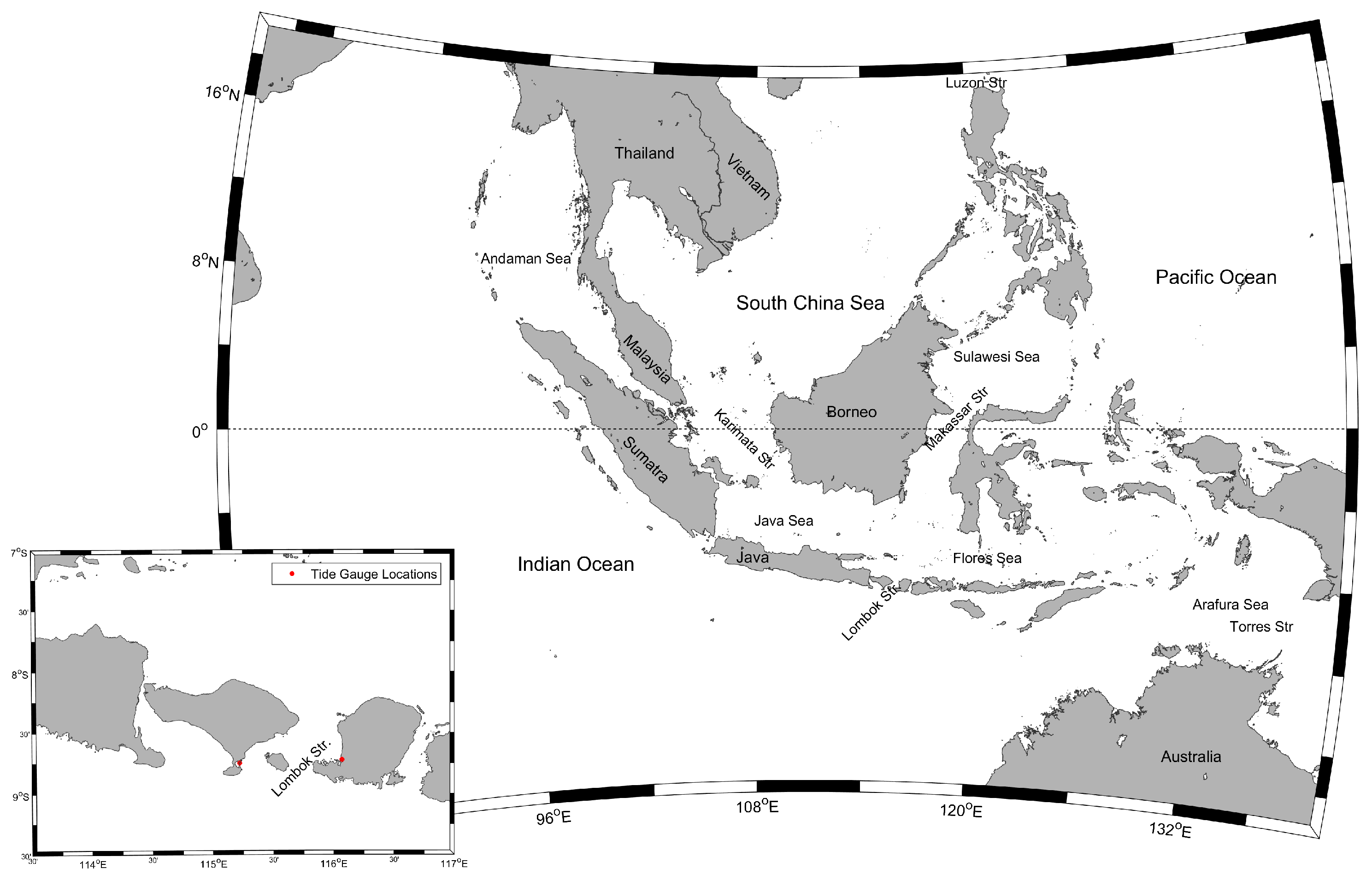
1.2. Indonesia’s Tides
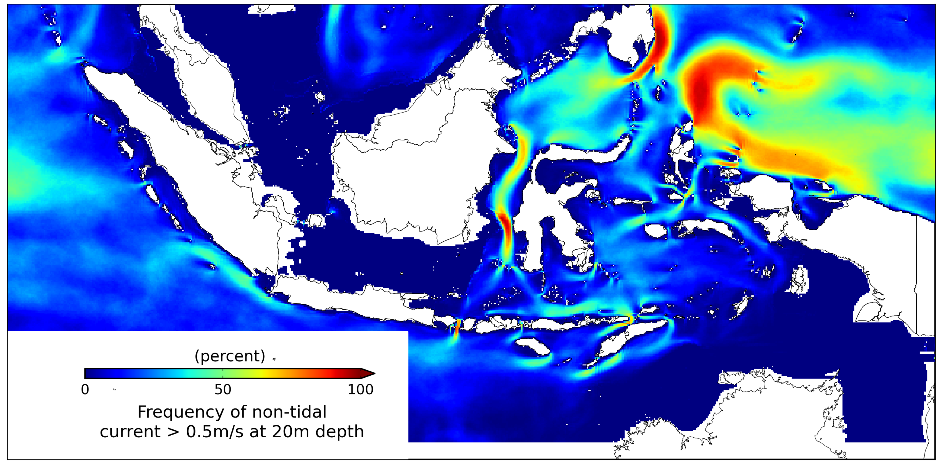
1.3. Indonesia’s Tidal Energy Resource
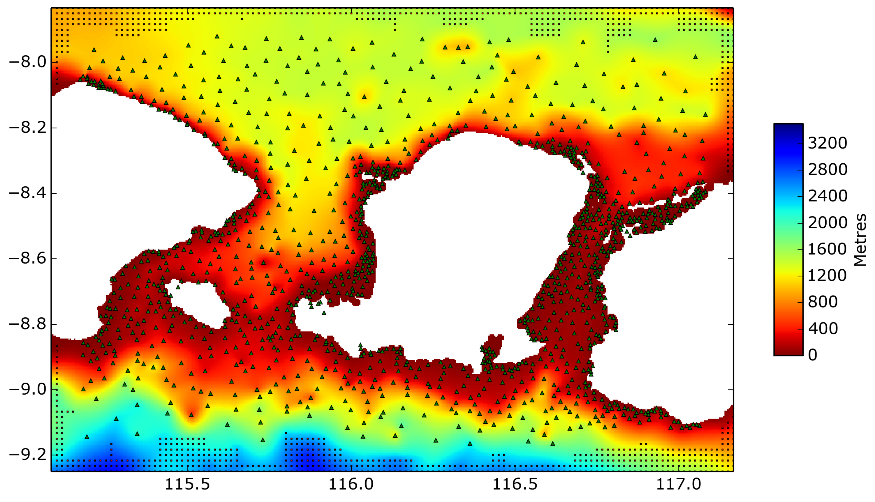
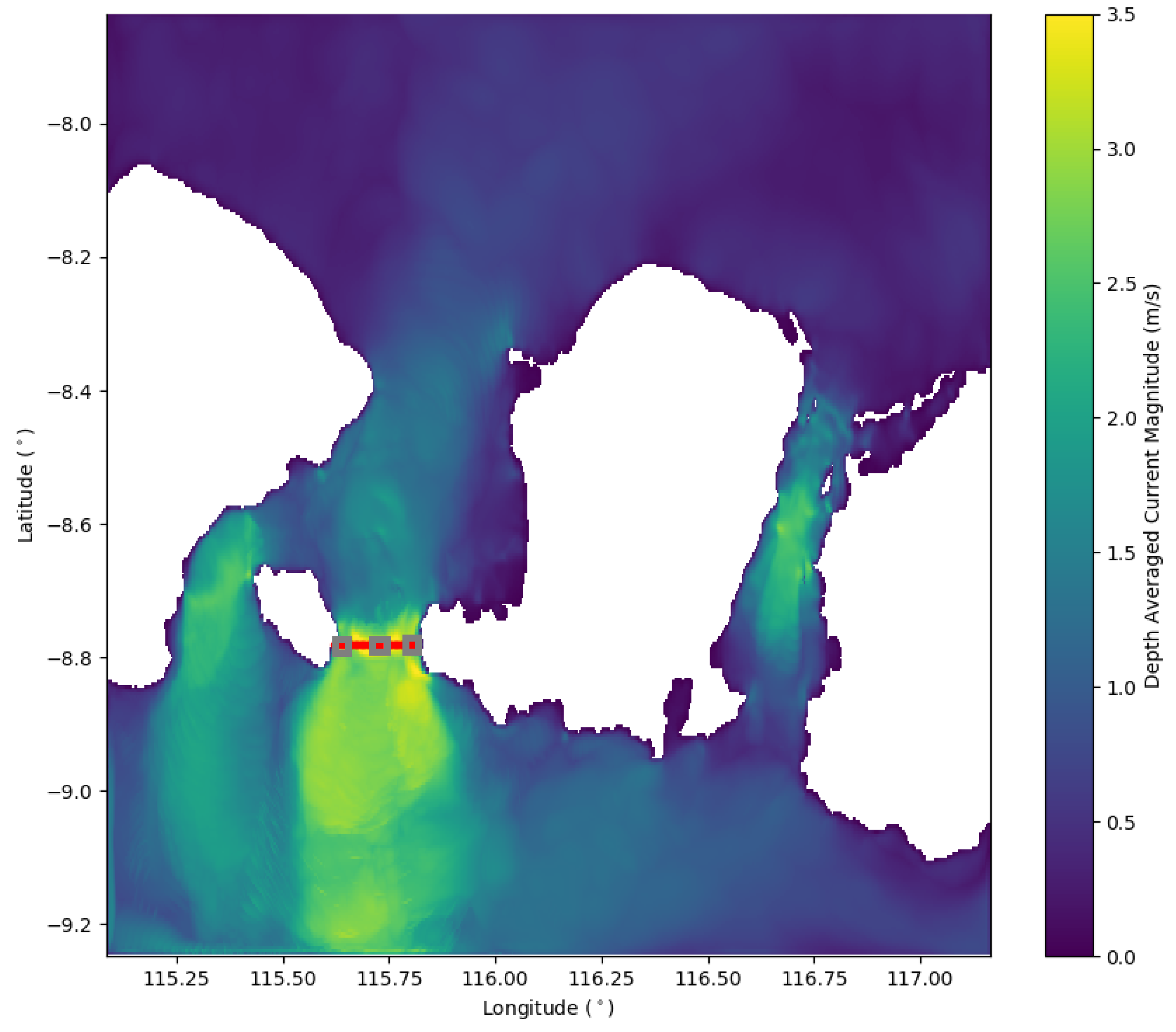
2. Materials and Methods
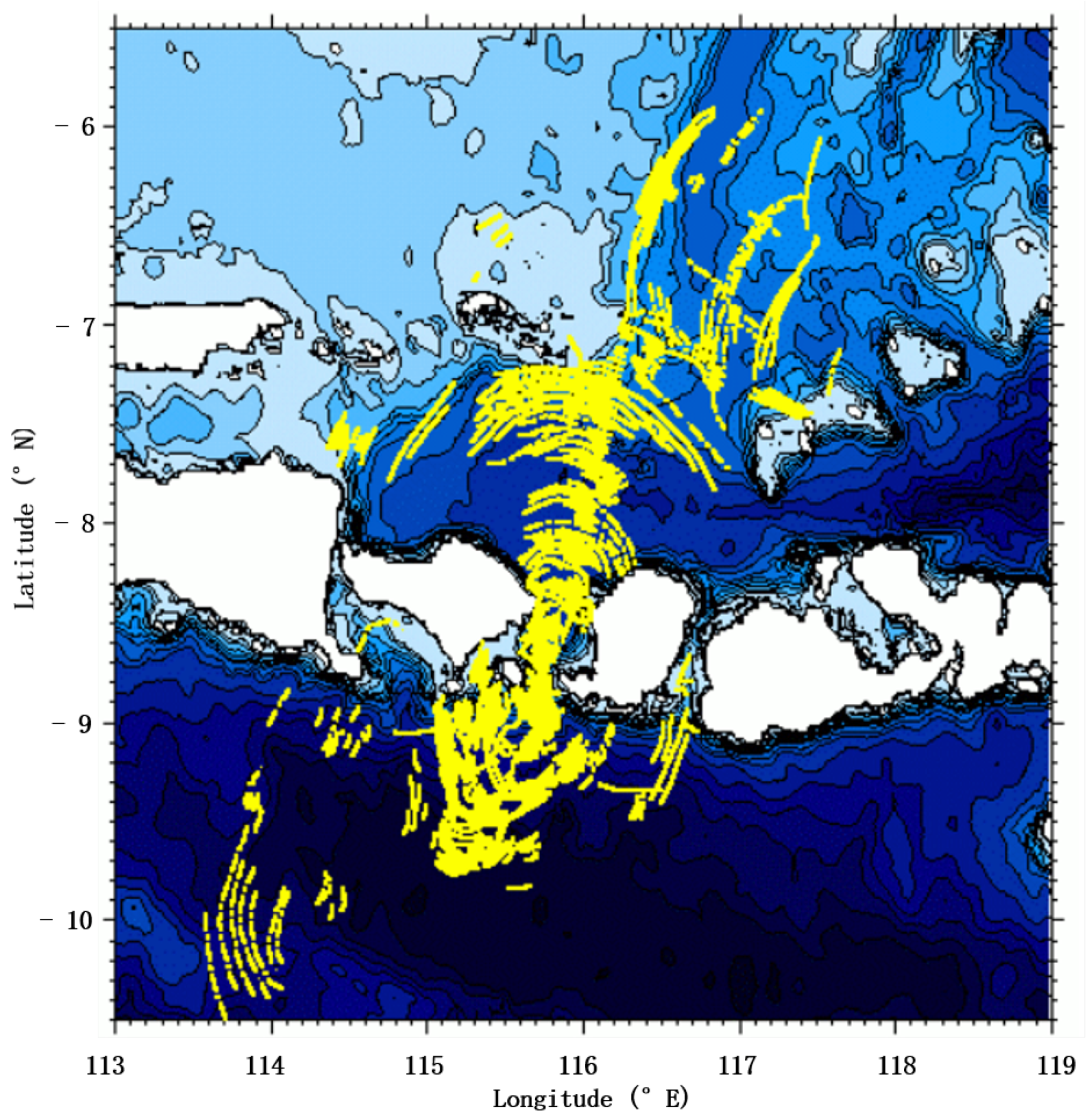
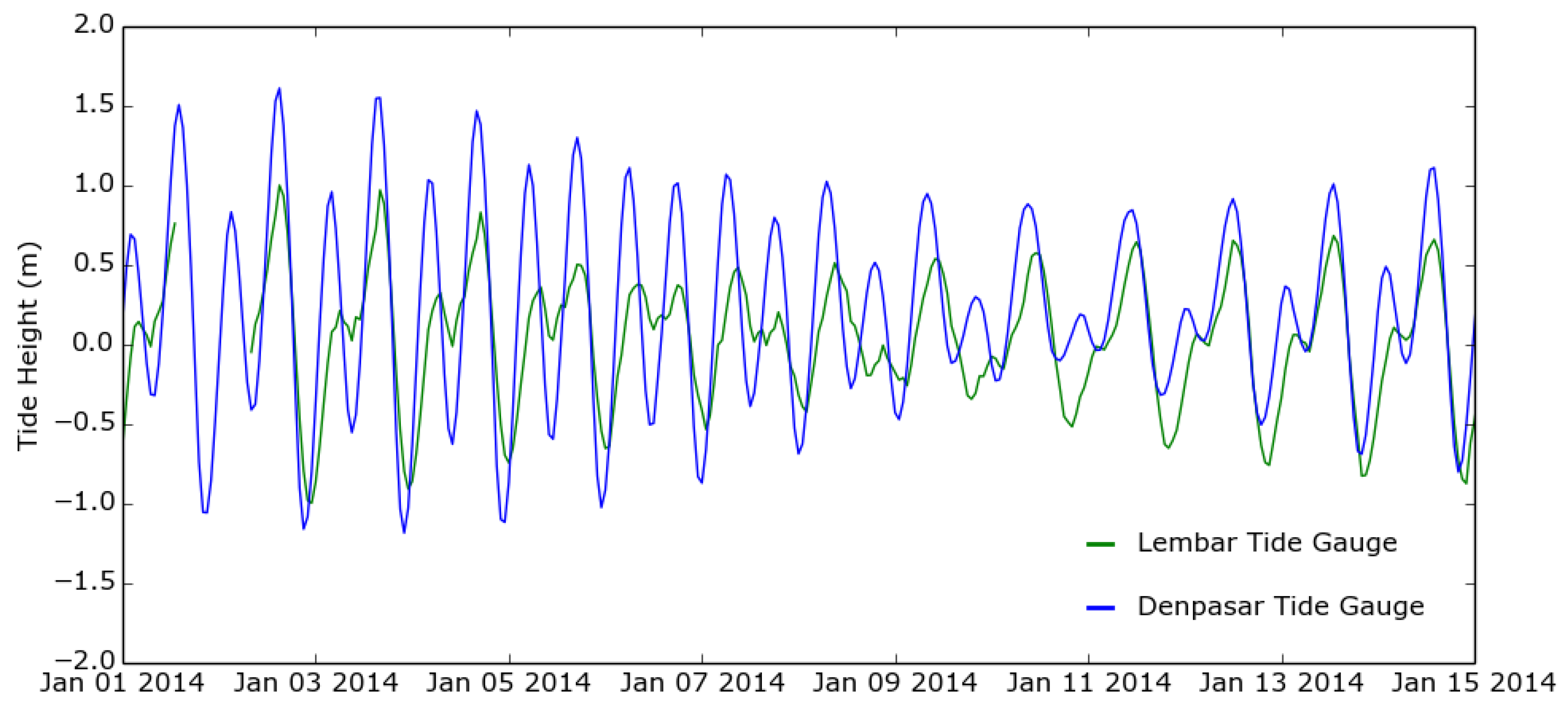
Model Validation
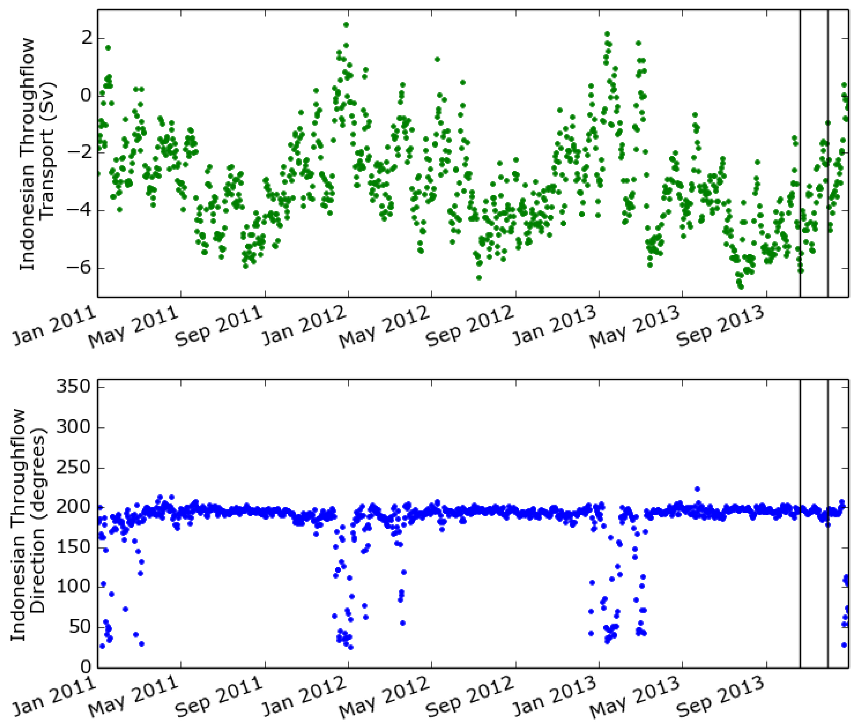
3. Results
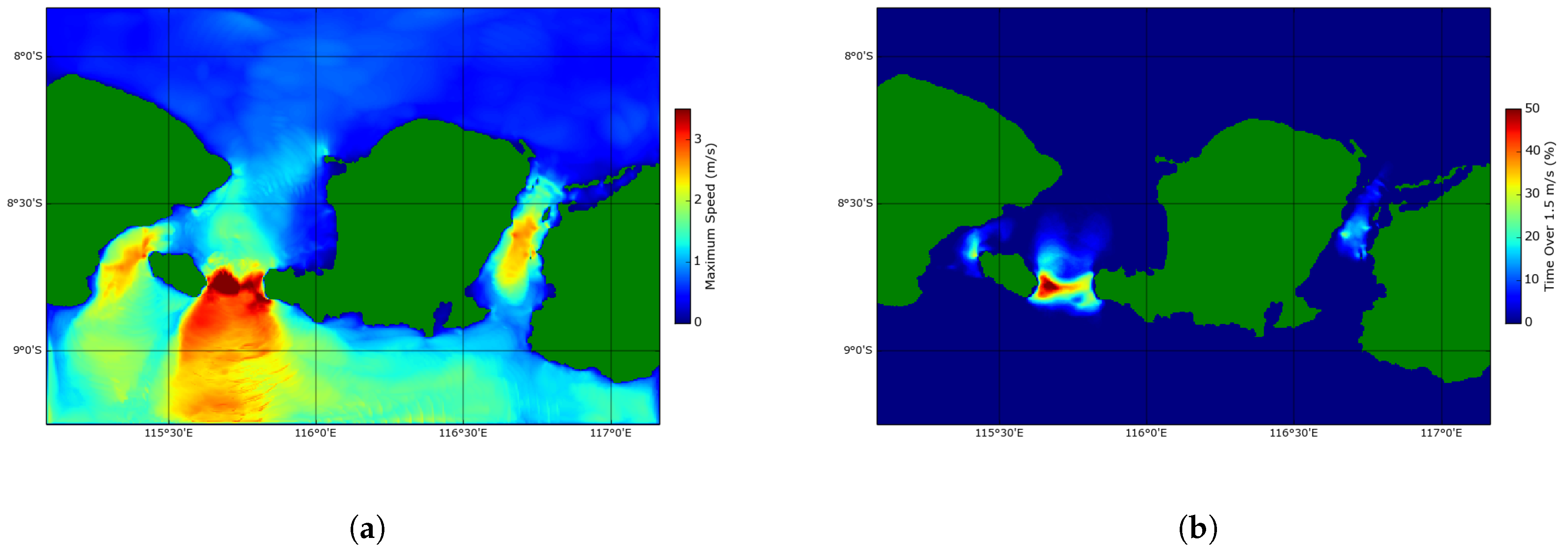
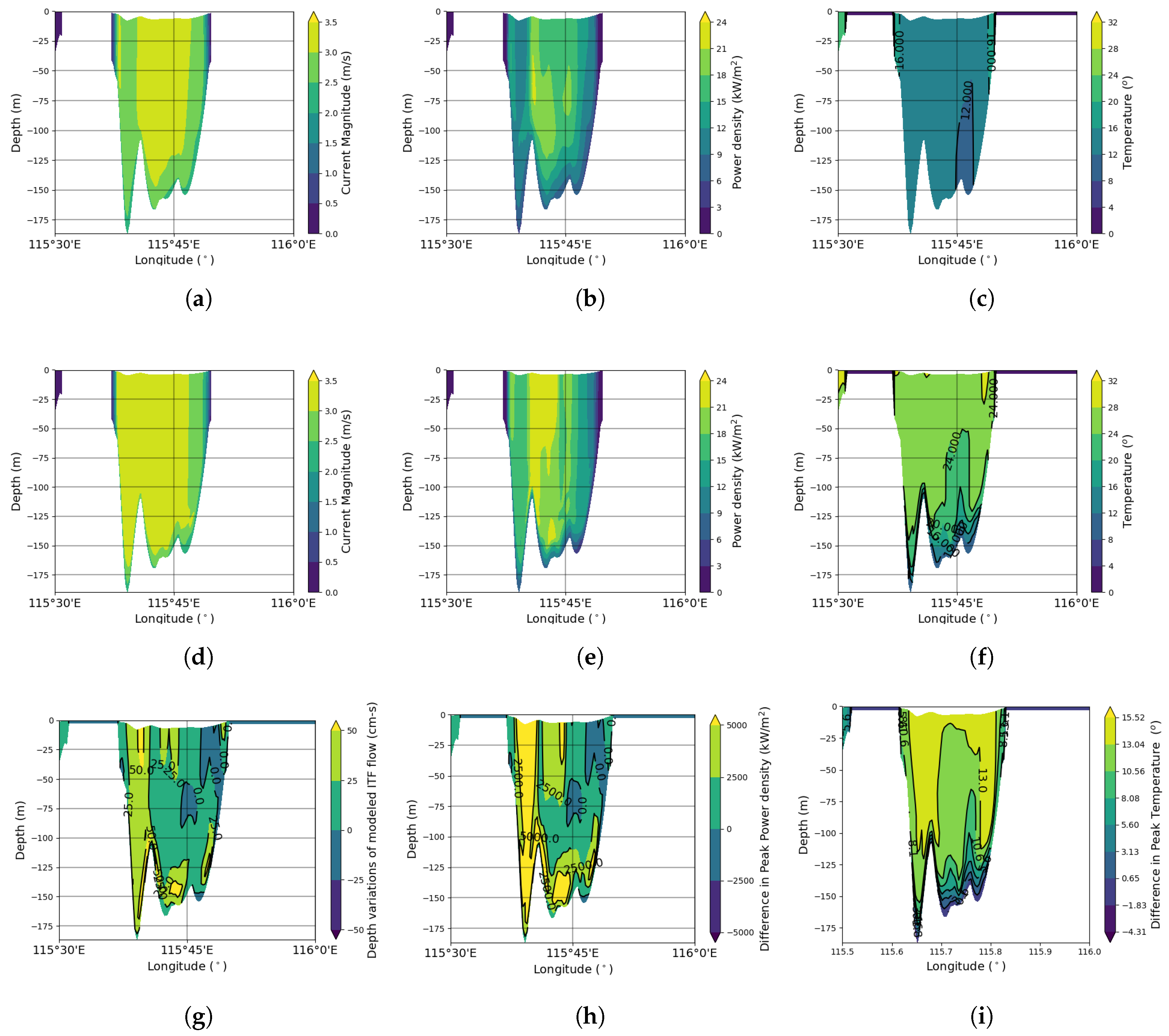
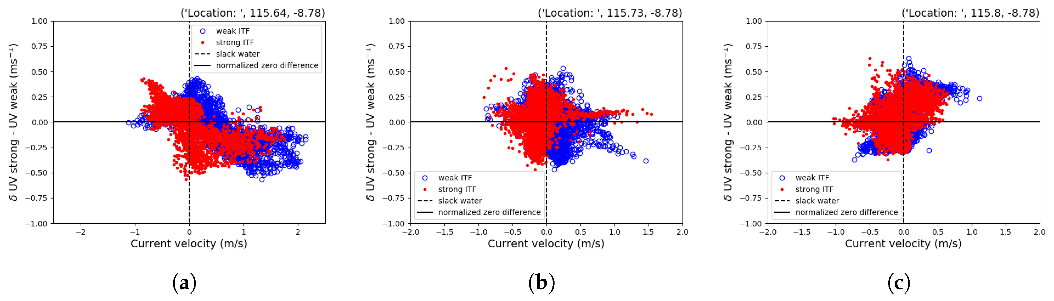
How Does the ITF Influence the Lombok Strait Tidal Resource?
4. Discussion
5. Conclusions
Author Contributions
Funding
Acknowledgments
Conflicts of Interest
Abbreviations
| GHG | Greenhouse Gas |
| ITF | Indonesian Through Flow |
| ROMS | Regional Ocean Modeling System |
| HYCOM | HYbrid Coordinate Ocean Model |
| OTPS | Oregon State University Tidal Prediction Software |
| RMSE | Root Mean Square Error |
| FES | Finite Element Solution |
| ROMS TO | ROMS Tide Only Simulation |
| ROMS ITF | ROMS Simulation Including the Indonesian Through Flow |
| POM | Princeton Ocean Model |
References
- Handayani, K.; Krozer, Y.; Filatova, T. Trade-offs between electrification and climate change mitigation: An analysis of the Java-Bali power system in Indonesia. Appl. Energy 2017, 208, 1020–1037. [Google Scholar] [CrossRef]
- Tharakan, P. Summary of Indonesia’s Energy Sector Assessment; ADB Indonesia: Metro Manila, Philippines, 2015. [Google Scholar]
- Firdaus, A.M.; Houlsby, G.T.; Adcock, T.A. Opportunities for Tidal Stream Energy in Indonesian Waters. In Proceedings of the 12th European Wave and Tidal Energy Conference, Cork, Ireland, 27 August–1 September 2017. [Google Scholar]
- Blunden, L.S.; Bahaj, A.S.; Aziz, N.S. Tidal current power for Indonesia? An initial resource estimation for the Alas Strait. Renew. Energy 2013, 49, 137–142. [Google Scholar] [CrossRef]
- Encyclopædia Britannica. Indonesia. Available online: https://www.britannica.com/place/Indonesia (accessed on 22 July 2019).
- Wyrtki, K. Indonesian through flow and the associated pressure gradient. J. Geophys. Res. Oceans 1987, 92, 12941–12946. [Google Scholar] [CrossRef]
- Jeans, G. Forecasting the Occurrence of Internal Solitons in Regions of Offshore Oil and Gas Activity; Oceanology International: London, UK, 2002. [Google Scholar]
- Mitnik, L.; Alpers, W.; Lim, H. Thermal plumes and internal solitary waves generated in the Lombok Strait studied by ERS SAR. In Proceedings of the ERS-Envisat Symposium: Looking down to Earth in the New Millennium, Gothenburg, Sweden, 16–20 October 2000; pp. 16–20. [Google Scholar]
- Kuswardani, R.T.D.; Qiao, F. Influence of the Indonesian Throughflow on the upwelling off the east coast of South Java. Chin. Sci. Bull. 2014, 59, 4516–4523. [Google Scholar] [CrossRef]
- Fang, G.; Wang, Y.; Wei, Z.; Fang, Y.; Qiao, F.; Hu, X. Interocean circulation and heat and freshwater budgets of the South China Sea based on a numerical model. Dyn. Atmos. Oceans 2009, 47, 55–72. [Google Scholar] [CrossRef]
- Gordon, A.L.; Fine, R.A. Pathways of water between the Pacific and Indian oceans in the Indonesian seas. Nature 1996, 379, 146. [Google Scholar] [CrossRef]
- Robins, P.E.; Neill, S.P.; Lewis, M.J.; Ward, S.L. Characterising the spatial and temporal variability of the tidal-stream energy resource over the northwest European shelf seas. Appl. Energy 2015, 147, 510–522. [Google Scholar] [CrossRef] [Green Version]
- Pawlowicz, R.; Beardsley, B.; Lentz, S. Classical tidal harmonic analysis including error estimates in MATLAB using T_TIDE. Comput. Geosci. 2002, 28, 929–937. [Google Scholar] [CrossRef]
- Cornett, A.; Toupin, M.; Nistor, I. Appraisal of IEC technical specification for tidal energy resource assessment at Minas Passage, Bay of Fundy, Canada. In Proceedings of the 11th European Wave and Tidal Energy Conference, Nantes, France, 6–11 September 2015. [Google Scholar]
- Neill, S.P.; Hashemi, M.R.; Lewis, M.J. The role of tidal asymmetry in characterizing the tidal energy resource of Orkney. Renew. Energy 2014, 68, 337–350. [Google Scholar] [CrossRef]
- Warner, J.C.; Sherwood, C.R.; Signell, R.P.; Harris, C.K.; Arango, H.G. Development of a three-dimensional, regional, coupled wave, current, and sediment-transport model. Comput. Geosci. 2008, 34, 1284–1306. [Google Scholar] [CrossRef]
- Amante, C.; Eakins, B.W. ETOPO1 Arc-Minute Global Relief Model: Procedures, Data Sources and Analysis; NOAA Technical Memorandum NESDIS NGDC-24; National Geophysical Data Center, Marine Geology and Geophysics Division: Boulder, CO, USA, March 2009.
- Egbert, G.D.; Erofeeva, S.Y. Efficient inverse modeling of barotropic ocean tides. J. Atmos. Ocean. Technol. 2002, 19, 183–204. [Google Scholar] [CrossRef]
- Dee, D.P.; Uppala, S.; Simmons, A.; Berrisford, P.; Poli, P.; Kobayashi, S.; Andrae, U.; Balmaseda, M.; Balsamo, G.; Bauer, P.; et al. The ERA-Interim reanalysis: Configuration and performance of the data assimilation system. Q. J. R. Meteorol. Soc. 2011, 137, 553–597. [Google Scholar] [CrossRef]
- Metzger, E.; Hurlburt, H.; Xu, X.; Shriver, J.F.; Gordon, A.; Sprintall, J.; Susanto, R.v.; Van Aken, H. Simulated and observed circulation in the Indonesian Seas: 1/12 global HYCOM and the INSTANT observations. Dyn. Atmos. Oceans 2010, 50, 275–300. [Google Scholar] [CrossRef]
- Susanto, R.; Mitnik, L.; Zheng, Q. Ocean internal waves observed in the Lombok Strait. Oceanography 2005, 18, 80–87. [Google Scholar] [CrossRef]
- Orhan, K.; Mayerle, R.; Narayanan, R.; Pandoe, W. Investigation of the Energy Potential From Tidal Stream Currents In Indonesia. Coast. Eng. Proc. 2017, 1, 10. [Google Scholar] [CrossRef]
- Carrere, L.; Lyard, F.; Cancet, M.; Guillot, A. FES 2014, a new tidal model—Validation results and perspectives for improvements. In Proceedings of the ESA Living Planet Symposium, Prague, Czech Republic, 9–13 May 2016. [Google Scholar]
- Ray, R.D.; Susanto, R.D. A fortnightly atmospheric ‘tide’at Bali caused by oceanic tidal mixing in Lombok Strait. Geosci. Lett. 2019, 6, 6. [Google Scholar] [CrossRef]
- Lewis, M.; Neill, S.; Hashemi, M.; Reza, M. Realistic wave conditions and their influence on quantifying the tidal stream energy resource. Appl. Energy 2014, 136, 495–508. [Google Scholar] [CrossRef] [Green Version]


© 2019 by the authors. Licensee MDPI, Basel, Switzerland. This article is an open access article distributed under the terms and conditions of the Creative Commons Attribution (CC BY) license (http://creativecommons.org/licenses/by/4.0/).
Share and Cite
Goward Brown, A.J.; Lewis, M.; Barton, B.I.; Jeans, G.; Spall, S.A. Investigation of the Modulation of the Tidal Stream Resource by Ocean Currents through a Complex Tidal Channel. J. Mar. Sci. Eng. 2019, 7, 341. https://doi.org/10.3390/jmse7100341
Goward Brown AJ, Lewis M, Barton BI, Jeans G, Spall SA. Investigation of the Modulation of the Tidal Stream Resource by Ocean Currents through a Complex Tidal Channel. Journal of Marine Science and Engineering. 2019; 7(10):341. https://doi.org/10.3390/jmse7100341
Chicago/Turabian StyleGoward Brown, Alice J., Matt Lewis, Benjamin I. Barton, Gus Jeans, and Steven A. Spall. 2019. "Investigation of the Modulation of the Tidal Stream Resource by Ocean Currents through a Complex Tidal Channel" Journal of Marine Science and Engineering 7, no. 10: 341. https://doi.org/10.3390/jmse7100341