Article

Coastal Flooding Caused by Extreme Coastal Water Level at the World Heritage Historic Keta City (Ghana, West Africa)

by
Emmanuel K. Brempong
1,2,3,*,
Rafael Almar
2,
Donatus Bapentire Angnuureng
1,
Precious Agbeko Dzorgbe Mattah
1,
Philip-Neri Jayson-Quashigah
4,
Kwesi Twum Antwi-Agyakwa
1,2 and
Blessing Charuka
1,2
1
Africa Centre of Excellence in Coastal Resilience (ACECoR), University of Cape Coast, Cape Coast 00223, Ghana
2
Laboratoire d’Etudes en Géophysique et Océanographie Spatiales (LEGOS), Université de Toulouse/CNRS/CNES/IRD, 31400 Toulouse, France
3
Department of Fisheries and Aquatic Sciences, School of Biological Sciences, University of Cape Coast, Cape Coast 00233, Ghana
4
Institute for Environment and Sanitation Studies, University of Ghana, Legon Box LG 209, Ghana
*
Author to whom correspondence should be addressed.
J. Mar. Sci. Eng. 2023, 11(6), 1144; https://doi.org/10.3390/jmse11061144
Submission received: 25 April 2023 / Revised: 23 May 2023 / Accepted: 25 May 2023 / Published: 30 May 2023

Abstract

:
Like low-lying sandy coasts around the world, the Ghanaian coast is experiencing increasingly frequent coastal flooding due to climate change, putting important socioeconomic infrastructure and people at risk. Our study assesses the major factors contributing to extreme coastal water levels (ECWLs) from 1994 to 2015. ECWLs are categorized into low, moderate, and severe levels corresponding to the 30th, 60th, and 98th percentiles, respectively. Using these three levels over the Pleiades satellite-derived digital elevation model topography, potential flood extent zones are mapped. ECWLs have the potential to flood more than 40% of the study area, including socioeconomically important sites such as tourist beach resorts, Cape St. Paul lighthouse, and Fort Prinzenstein. In this study, all coastal flooding events recorded by the municipality of Keta fall within the 98th percentile category. Our results show a gradual increase in the frequency of flooding over the years. Flooding events are caused by a compound effect of the tide, sea level anomaly, waves, and atmospheric conditions. Finally, while wave run-up is the major contributor to coastal flooding, the tide is the one varying most, which facilitates a simple early warning system based on waves and tide but adds uncertainty and complicates long-term predictability.

1. Introduction

Globally, coastal flooding affects coastal areas due to sea level rise (SLR). Coastal areas serve as homes for about 2.4 billion people (40% of the world’s population) [1], as well as provide high economic value to coastal countries [2]. Over the 21st century, projections have shown that SLR would increase the rate of coastal flooding globally [3]. This would possibly displace most people living in low-lying coastal zones and impact socioeconomic and ecological systems of great importance, particularly in Africa [4,5]. Generally, the main cause of coastal flooding is high water levels due to several factors. Coastal flooding is instigated by an amalgamation of numerous factors from the ocean and atmosphere, such as mean sea level changes, tides, storm surges, waves, river discharge, and rainfall [6]. When two or more of these factors occur simultaneously, the severity of flooding can worsen, leading to an amplified risk of coastal flooding. Examples of compound flooding events include river discharge and surges [7], rainfall and surges [8] on the coast of the United States, and rainfall, surge, and waves [9,10]. If these events are statistically dependent, meaning they share a mutual driving force, the likelihood of them occurring together is higher than expected when considering each variable separately. This increased likelihood of compound flooding events can lead to a higher chance of coastal flooding [6,11].
All these together would eventually lead to overtopping and inundating coastal defenses in low-lying areas, which potentially cause damage to life and property. Coastal flooding continues to pose a huge threat to coastal inhabitants. It is known to be one of the most dangerous and costly of natural disasters [12,13]. Therefore, it is essential to create awareness of the need to plan, mitigate, and consider alternatives to reduce the effects of coastal flooding. Understanding the occurrence of extreme coastal water levels (ECWLs) [11,14] can help support decision making in coastal zone management. This would help identify regions affected by a strong increase in flood risk and prioritize mitigation and adaptation efforts [15]. During ECWLs, overtopping is the main cause of coastal flooding, with much water surpassing the maximum coastal elevation (e.g., dunes, dykes, cliffs) [16]. Despite this, when overtopping occurs, all areas with low elevation do not submerge though this phenomenon mainly drives localized coastal flooding and damage to infrastructures.
Furthermore, overtopping due to ECWLs is even more catastrophic when there is a failure or absence of coastal protection, such as groins and revetments [17]. According to [18], the principal components of ECWLs are sea level anomaly (SLA), dynamic atmospheric conditions (DACs), tide (T), and wave run-up (R). On the Jamestown Beach in Accra, [19] noted that shoreline change responds in decreasing order to sea level variations (86%), waves (9%), and tidal cycles (5%) on daily bases. Wind-induced setup has limited effect on the shoreline, while the observed most important component of SLA at that coast was the influence from the inverse barometer. SLA is due to the steric effect, ocean circulation, and transfer of mass from the continents (ice sheets, glaciers, land water) to the ocean, DACs due to atmospheric pressure and winds, astronomical tide (T), and wave effects here referred to collectively as run-up (R), which includes a time-averaged component (setup) and an oscillatory component (swash) [18]. Quantifying these local contributions during flooding events is key, as their relative contribution varies spatiotemporally. One key factor to consider when assessing flooding and overtopping is a suitable and higher DEM resolution. A higher-resolution DEM tends to preserve the topographical terrain features thus determining where floods are most likely to cause problems for people and property and estimating how water interacts with the environment depending on high-quality DEM data. The precision and spatial resolution of the DEM affect the accuracy of forecasts of flood depths [20]. Numerous publications have extensively examined the justification for utilizing coarse DEM resolutions. They came to a conclusion that, despite their lack of precision, their model simulations offer a suitable trade-off between readily accessible (free) data, minimal computational requirements, and an appropriate depiction of hydrological processes and catchment responses. However, even while increased spatial resolution and accuracy frequently lead to better outcomes, it is rarely available since these are commercial and not freely available. Recently, the high-resolution DEMs from sources such as Pleiades stereo imagery have played a significant role in coastal morphology changes, making them a great tool to explore and use [21,22].
The eastern coast of Ghana is known to be the most vulnerable coast in Ghana. It experiences coastal flooding not less than twice every year [23]. In addition, the frequency and intensity of coastal flooding and erosion have increased. Over the past decade, the Volta Delta has significantly experienced coastal flooding events and duration [23,24,25]. Some studies have attributed this to intensive rainfall, oceanographic conditions (waves, sea level rise, and tides), and human activities (watershed management) [23].
On the other hand, the construction of the Akosombo dam on the Volta River has been identified as a major cause of erosion and flooding problems in the Volta Delta region [26,27,28]. In particular, the Keta District has been affected by coastal erosion and flooding. For this reason, one of Ghana’s largest sea defenses was constructed from 2000 to 2004 to control coastal erosion and flooding. Therefore, it is very important to understand hydrodynamic factors dominating coastal flooding in Keta and Volta Delta at large.
Our study uses Pleiades stereo images to develop the digital elevation model (DEM) and wave, tide, and sea level anomaly data from satellite and globally freely available reanalysis. The main aim of this study is to assess the predominant factors of coastal flooding in the Keta municipality. To achieve this, ECWLs were first categorized into three main percentiles (30th, 60th, and 98th); secondly, the spatial extent of flooding at each percentile was assessed; and finally, the dominant and most varying factors were assessed in the 98th percentile scenario. The importance of this study is that it explores the most dominant factors and thus provides reasons to consider these factors in implementing coastal flooding decisions.

2. Materials and Methods
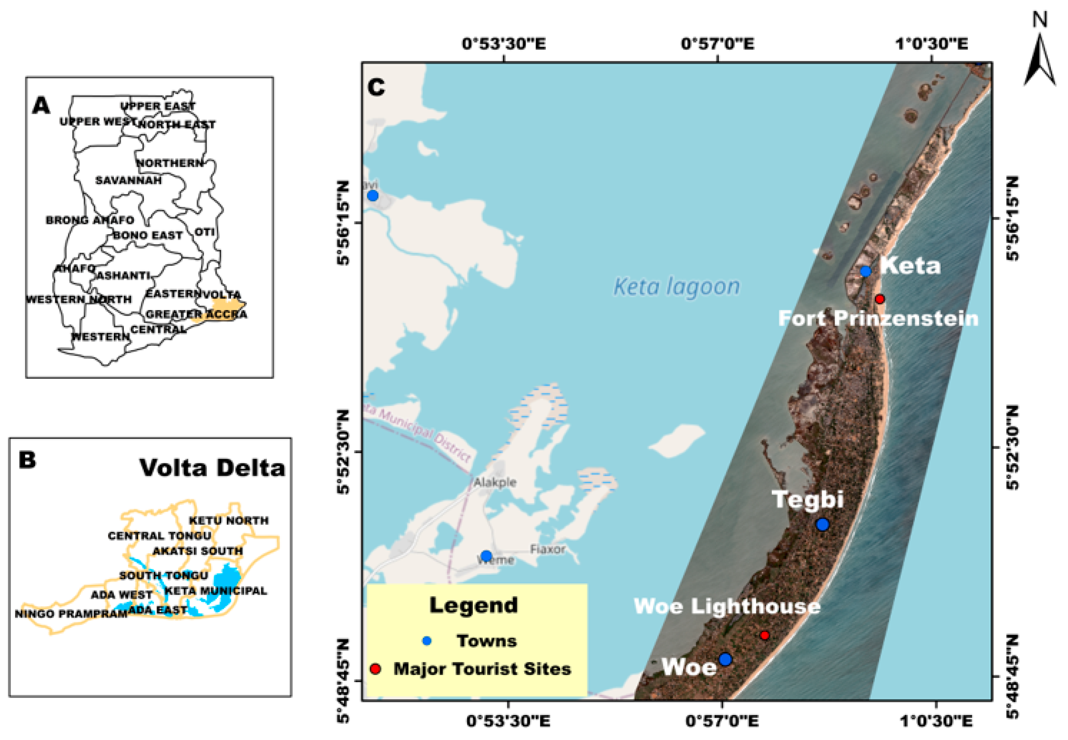
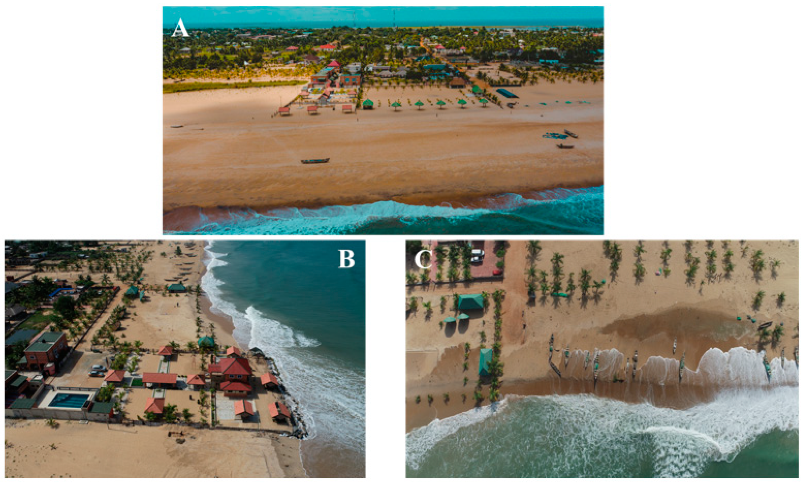
2.1. Study Area

Keta City is located in a large wetland-protected area of 1200 km2. Keta lies on the eastern coast of Ghana and is located precisely at the extreme east of the Volta Estuary. This study used Pleiades satellite imagery (Figure 1c) covering major towns such as Woe, Tegbi, and Keta. The largest lagoon in Ghana, the Keta Lagoon complex, is located in this municipality. The Keta Lagoon facilitates water transportation to surrounding communities and has the potential for large-scale commercial aquaculture. Generally, the municipality serves as a breeding ground for many sea turtles and a temporary passage point for migratory birds. The town is separated by a narrow sand strip separating the Keta Lagoon from the sea. Keta is in the Keta Basin, and its geology largely includes mud, wabbly sand, and gravel [29]. Studies by [30] indicate the presence of numerous canyons (valleys) in the deep waters, which also signify active erosion. In the past, rampant coastal flood and erosion cases were recorded, precisely in 1907 when the first coastal erosion occurred, then in 1924, 1949, 1986, 1996, and 1997 [31]. This has led to the construction of sea defense structures along the Keta municipality stretch.
The climate conditions are dry equatorial, with a mean rainfall below 1000 mm in May and July and sometimes late August and October. Generally, wind conditions are weak, with speeds less than 2.6 m/s [32,33]. Wave conditions are generally less than 3 m and a maximum period of 19.68 s in the direction south and southwest with an average period of 10.91 s. The tide condition is micro-tidal and estimated to be 1 m on average. The beaches are generally sandy with a median grain size of 0.6 mm, and most inhabitants survive by fishing and farming [34]. The inhabitants of Keta District are involved in various economic activities. These include agriculture, fisheries, salt harvesting, sand mining, and tourism. The agricultural and fishing sectors are more dominant than the other sectors. Fort Prizenstein and Woe Lighthouse are two major tourist sites in the Keta District. The Keta District is very important to the Volta Delta; therefore, it is imperative to assess and understand the factors that influence coastal flooding in this area and for the Volta Delta as a whole.

2.2. Datasets

This section describes the data used for this study. This study uses satellite imagery and hydrodynamic data for the Keta area.

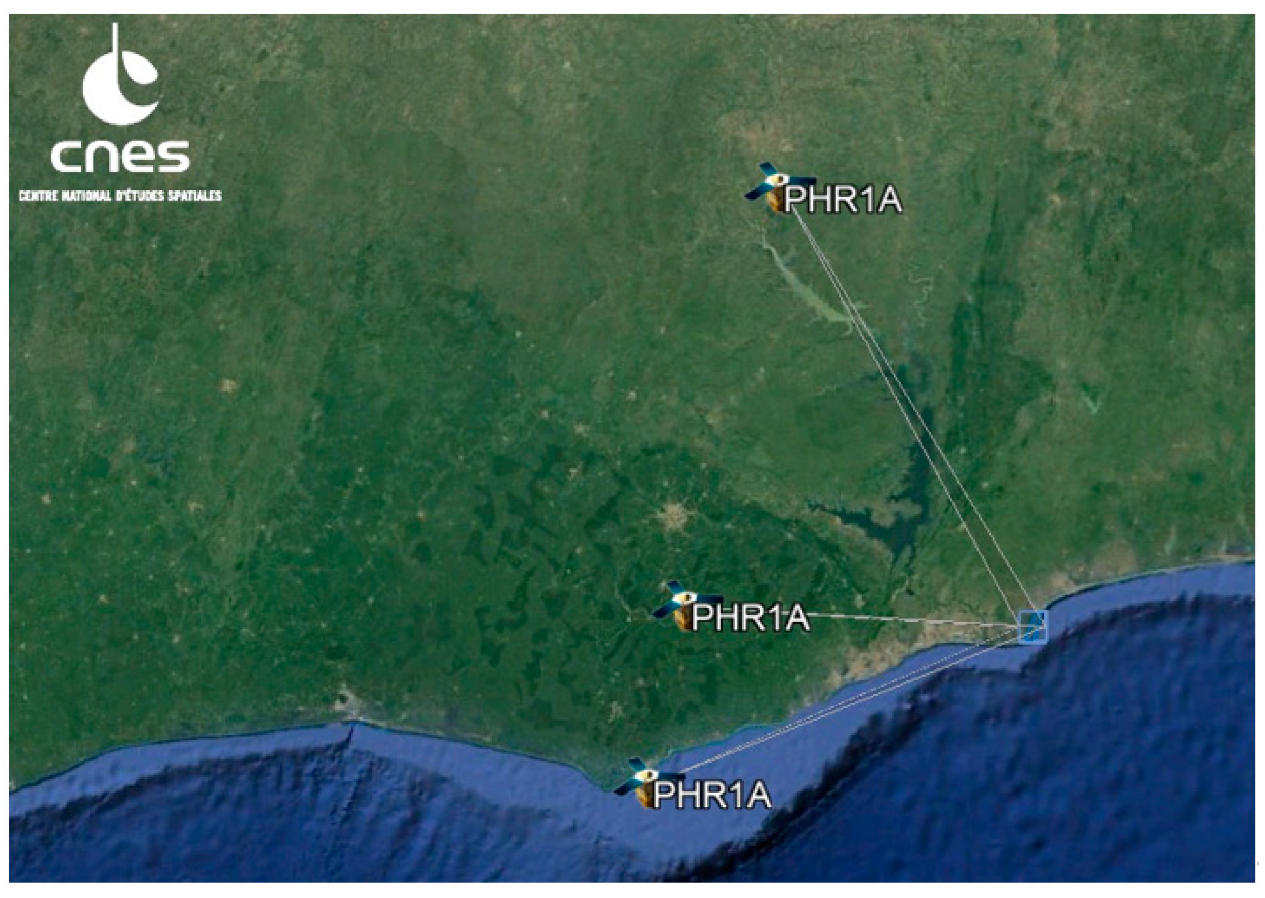
2.2.1. Pleiades Satellite Imagery and Acquisition

Satellite data provide key missing information for coastal management [35,36], including ocean drivers, land use, and vulnerability assessment [18,33].
It turns out that in West Africa, there are several gaps in coastal management. In addition, there is limited use of high-resolution satellites, thereby preventing any efficient mitigation measure on a broad scale.
The Pleiades satellites 1A and 1B were launched in 2011 and 2012, respectively, at an altitude of 694 km and can obtain a burst of up to 12 images during a single pass [37]. The Pleiades imagery comes in single or (tri)stereo images with panchromatic and multi-spectral images of respective ground pixel resolutions of 0.5 m and 2 m. Thus, the sensors of the Pleiades satellites work in the near-infrared and visible spectrum. However, the Pleiades imagery was first established in line with the French–Italian Optical and Radar Federated Earth Observation program (ORFEO). In recent years, other partners in Europe and other countries have used it in their studies. The major features of the Pleiades collection are explained in detail in the user guide of Pleiades imagery [38]. For this study, tri-stereo imagery was acquired from the Centre National D’etudes Spatiales (CNES).
At Keta, such burst and tri-stereo images (Figure 2) were acquired on 20 October 2020 and constituted the data used in this study. The time difference between the individual images is set for each acquisition to dT = 6 s. This gives a base-to-height (B-H) ratio for the two data sets of B/H = 0.12. Generally, for flat areas, a low B/H value provides better height accuracy of the stereoscopy [39]. The Pleiades images were acquired at an approximately equal tidal elevation of +0.8 m. These images were finally downloaded from Centre National D’etudes Spatiales (CNES) website. Unfortunately, these data are not freely available but were acquired with the help of LEGOS.

2.2.2. Hydrodynamic Data

To compute ECWLs, it is required to use hydrodynamic, meteorological, and tidal parameters [11]. For this study, the parameters used include; sea level anomaly (SLA), wave run-up (R), tide (T), and other atmospheric conditions (DACs). All parameters were referenced to the WGS84 datum and extracted at a grid point of latitude of 6.047366° and longitude of 1.080522°.
Tide data were extracted on the hourly resolution at the nearest grid point from the global tide FES (finite element solution) 2014 model [40]. These data were produced by the Laboratory of Geophysical and Oceanographic Spatial Studies of Toulouse (LEGOS). AVISO (Archiving, Validation and Interpretation of Satellite Oceanographic) data, with the support of the Centre National d’Etudes Spatiales (CNES), distributes the atmospheric pressure and winds component (DACs) generated by the MOG2D model from LEGOS of the Collecte Localisation Satellites (CLS) Space Oceanography Division [41]. More information can be found at http://www.aviso.altimetry.fr/ (accessed on 20 March 2022).
Altimetric-derived SLA, including global mean level rise (GMSLR), was extracted from AVISO’s nearest grided data point of the altimetry data point [42].
All wave run-up data were obtained from ERA-interim reanalysis (global climate and weather data available from 1979 onward) at a 0.5° × 0.5° resolution. These data were produced by the European Center for Medium-Range Weather Forecasting (ECMWF) model, which used wave data at 6-hourly resolution. The calculation of wave run-up (R) was performed using the dissipative beach equation proposed by [43] (see [11]).
R = 0.043√HsLo
Hs is the offshore significant wave height, and Lo is the wavelength. All the parameters mentioned above are resampled hourly from 1994 to 2015. All hydrodynamic data used in this study were freely available and extracted for the Keta area within its conforming grids.

2.3. Workflow and Methodology

This section describes all methods used in this study; this includes DEMs derived from the Pleiades, computing extreme coastal water levels (ECWLs), and flood extent mapping.

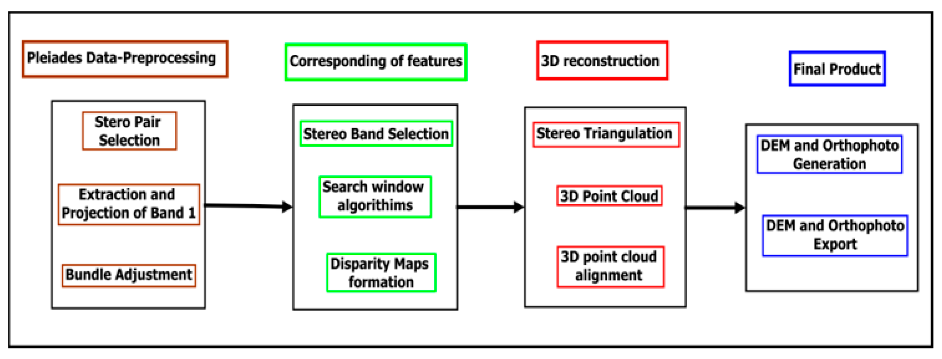
2.3.1. Pleiades-Derived Topography

Digital elevation models (DEMs) were generated from the Pleiades stereo imagery using the NASA AMES Stereo Pipeline (ASP) software to obtain the topographic variation of the beach. The ASP software uses the tri-stereogrammetry method, where DEMs are derived from the sensor level. For the tri-stereo methodology approach of ASP, three panchromatic images are taken as input (0.5 m resolution) [44]. These are then correlated pair by pair, and a final correlation between the two correlated pairs gives the output DEM. This method uses the rational polynomial coefficient (RPC), which accompanies the imagery and further provides a relationship between the satellite image and ground coordinates. The DEM was then orthorectified by referencing them to planimetric coordinates. This was performed using AMES Stereo Pipeline software. It has a feature that ortho-rectifies a sensor-level satellite image using its geometry by the accompanied RPC file and, in the process, creates a DEM at a set resolution (see also [21,22]). This DEM is automatically orthorectified, after which the satellite images at the sensor are projected onto the DEM so that the output images are fully orthorectified and corrected using ground control points [38]. The Pleiades panchromatic images (0.5 m resolution) produced a 2 m resolution DEM. The various steps involved in Pleiades imagery processing are summarized in Figure 3.

Pleiades Imagery Pre-Processing

This is the preliminary stage of Pleiades data processing. In this stage, data are selected and organized by matching similar features. The pairs of Pleiades images called 1 and 2 and 2 and 3 are selected and processed. After this, the stereo image pairs are selected, and band one is selected from each image and aligned using the affine-epipolar algorithm of ASP [45]. Images are pre-aligned. This process is carried out by identifying tie-points between them, which are then used to alternate the sensor spot to guarantee that pairs of conjugate epipolar lines are both col-linear and analogous to one of the image axes [46]. Due to the incompatibility of the ASP software with multi-band imagery, this study opted for a panchromatic image (band 1) as it offers a wide range of radiance data and suitable graphic and visual contrast, which aids in distinguishing image features from their respective shadows.

Corresponding of Features

In the ASP, features are matched with each other after the images are prepared for feature matching (Figure 3). The search window algorithms (SWs) in ASP approximates the superficial motion of each scene point by linking the search windows of each local window with each pixel in the stereo pair [47]. For each stereo pair, a relative disparity map is produced with a search window algorithm [45].

Reconstruction of Topography from Pleiades (3D Reconstruction)

After data are processed and corresponding features are identified, ASP uses the stereo triangulation algorithm method (Figure 3) to merge features to obtain a 3D location (x, y, z) of the nearby intersection between lines that link the sensor orbital location to all matched pixels in both the left and right images. This approach combines all the information on altitudes, the model of each sensor, and the disparity map. The result of the process is a raster format consisting of four bands containing triangulated coordinates for x, y, and z, as well as a triangulation error metric stored in the fourth band. This metric is useful in evaluating the quality of the sensor model, ephemeris/attitude data, and the disparity matches [41]. Next, the output is transformed into a 3D point cloud, which is geocoded using the WGS84 UTM 31N coordinate system and ellipsoid heights. The post-processing stage of the ASP involves determining the orthometric heights of the 3D point cloud using ground control points (GCPs) with known orthometric heights to calculate a height correction factor for the 3D point cloud [48]. Ground control points (GCPs) in the form of concrete pillars buried at ground level and marked for identification purposes were used for the study. These GCPs were obtained from [49] for the Keta area. The GCPs obtained were in the form of X, Y, and Zs of ground pillars. They were connected to the Ghana meter grid system to establish and coordinate the concrete pillars as ground control points (GCPs). This process followed the standards set by the Ghana Survey Department, ensuring consistency and conformity. The static differential GPS (D-GPS) method was employed to observe each control point, with an average observation time of not more than 30 min. These observations were referenced to the established Ghana national coordinated pillars [49]. Finally, the 3D point cloud is utilized to generate DEMs and orthophotos. The final DEM and orthophotos are exported and saved for further analysis using the ASP stereo-RPC algorithms.

2.3.2. The Altimeter Corrected Elevations Version 2 (ACE2)

To assess the quality of DEMs for coastal flooding studies, DEM was downloaded from the website of the Data Center in NASA’s Earth Observing System Data and Information System (EOSDIS). ACE2 is the second iteration of the global digital elevation model that the Shuttle Radar Topography Mission produced using satellite radar altimetry (SRTM). Version 1 data have been upgraded with the release of the Altimeter Corrected Elevations Version 2 (ACE2) generated by combining satellite radar altimetry with SRTM. Global Observations to Benefit the Environment (GLOBE), the original altimeter corrected elevations (ACEs) digital elevation model (DEM), and additional matrices produced by reprocessing European remote sensing (ERS-1) images are among the data sources used in the adjustment. The three arc seconds data (90 m) were downloaded with the same datum for this study to compare with Pleiades-derived DEM [50].

2.3.3. Computing Extreme Coastal Water Level (ECWL)

Using the hourly datasets described earlier, ECWLs were calculated hourly from 1994 to 2015. This approach followed the [7] formula.
ECWL = SLA + DAC + T + R
Three major percentiles were used to show how severe ECWLs go; the 30th, 60th, and 98th percentiles were obtained and further confirmed with in situ flood occurrence dates from 2000 to 2015 from the National Disaster Management Organization of the Keta District. In Keta, extreme coastal water levels (ECWLs) are determined using an approach that combines several parameters such as sea level anomaly (SLA), storm surge height caused by atmospheric pressure and winds (DACs), astronomical tide level (T), and height of wave breaking (R). The worst scenario of water levels is defined as the top 2% or 98th percentile to determine the physical impact of ECWLs in the area. The cumulative annual occurrence of the time spent over this threshold is computed over the study period. Topographic data are set to a geoidal coordinate system to assess the potential for overtopping and flooding. ECWLs are converted to geodetic data using the vertical datum value of [51] to superimpose with the topographic data. Finally, MATLAB software’s linear regression is used to analyze the trend of ECWLs in the Keta area based on annualized data.

2.3.4. Flood Extent Mapping

Potential flood extent zones were mapped using the bathtub inundation model. This approach assumes that areas would be flooded with elevations lower than the ECWL for all percentiles. Flooded areas are mapped in the geographic information system (GIS) environment using a simple calculation (Equation (3)). All elevations in each cell of the Pleiades DEM are equated against a predicted ECWL, and all cells that fall below the ECWL are considered flooded. Since only data on the elevation are needed for its application, the approach allows for estimates without detailed hydrological data [52].
Using the raster calculator tool in ArcGIS 10.4, ECWLs for the different percentiles were computed to assess areas that fall below ECWLs along Keta City. All ECWLs for the three percentiles were considered for a bathtub analysis. This approach is frequently used for this type of analysis [53,54,55,56]. The ESRI’s ArcGIS 10.4 and MATLAB software was used for statistical calculation and map development.
Elevation projection by ECWL(p) = (DEM ≤ ECWL (p))
where (p) are percentiles (30th, 60th, or 98th percentile).

3. Results

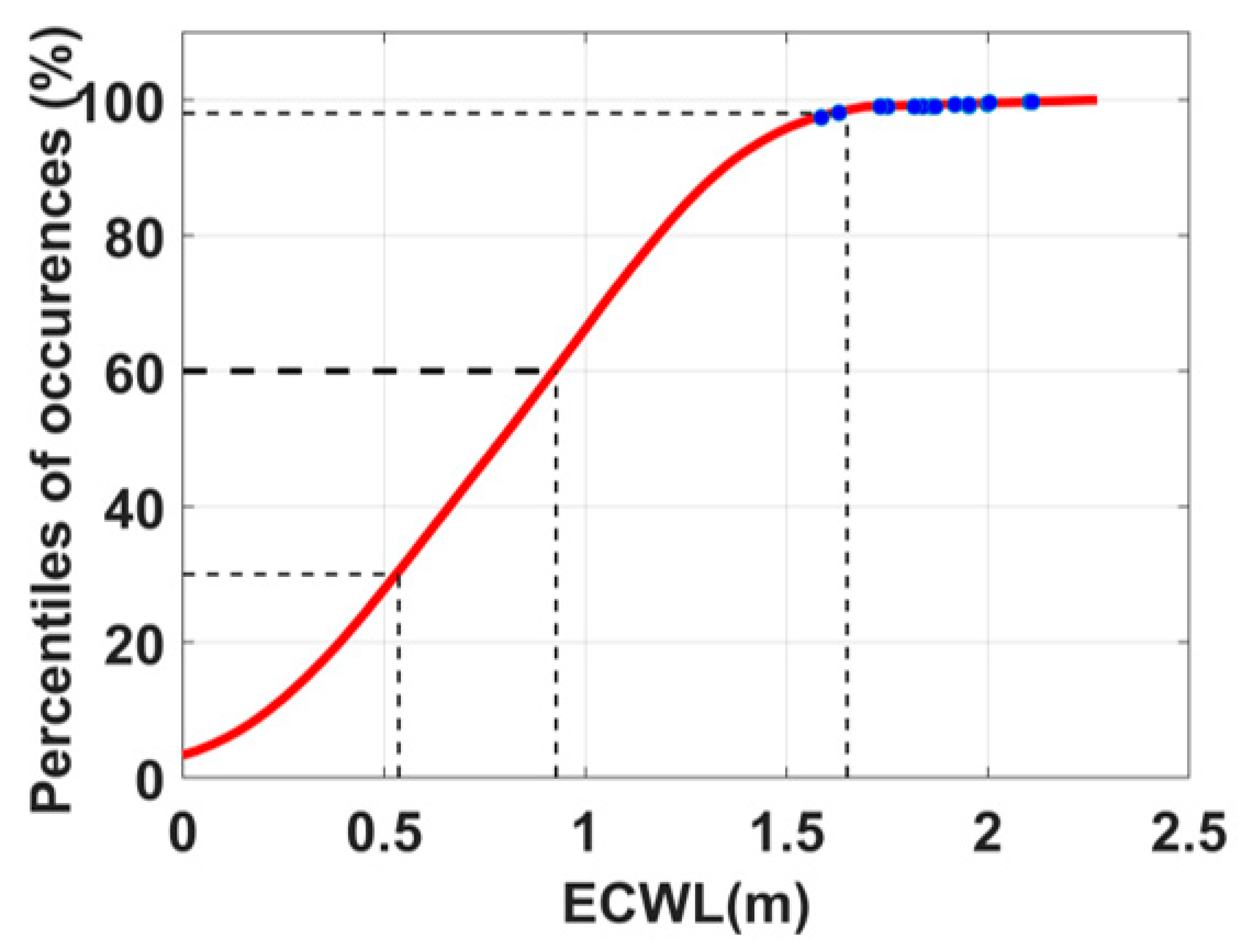
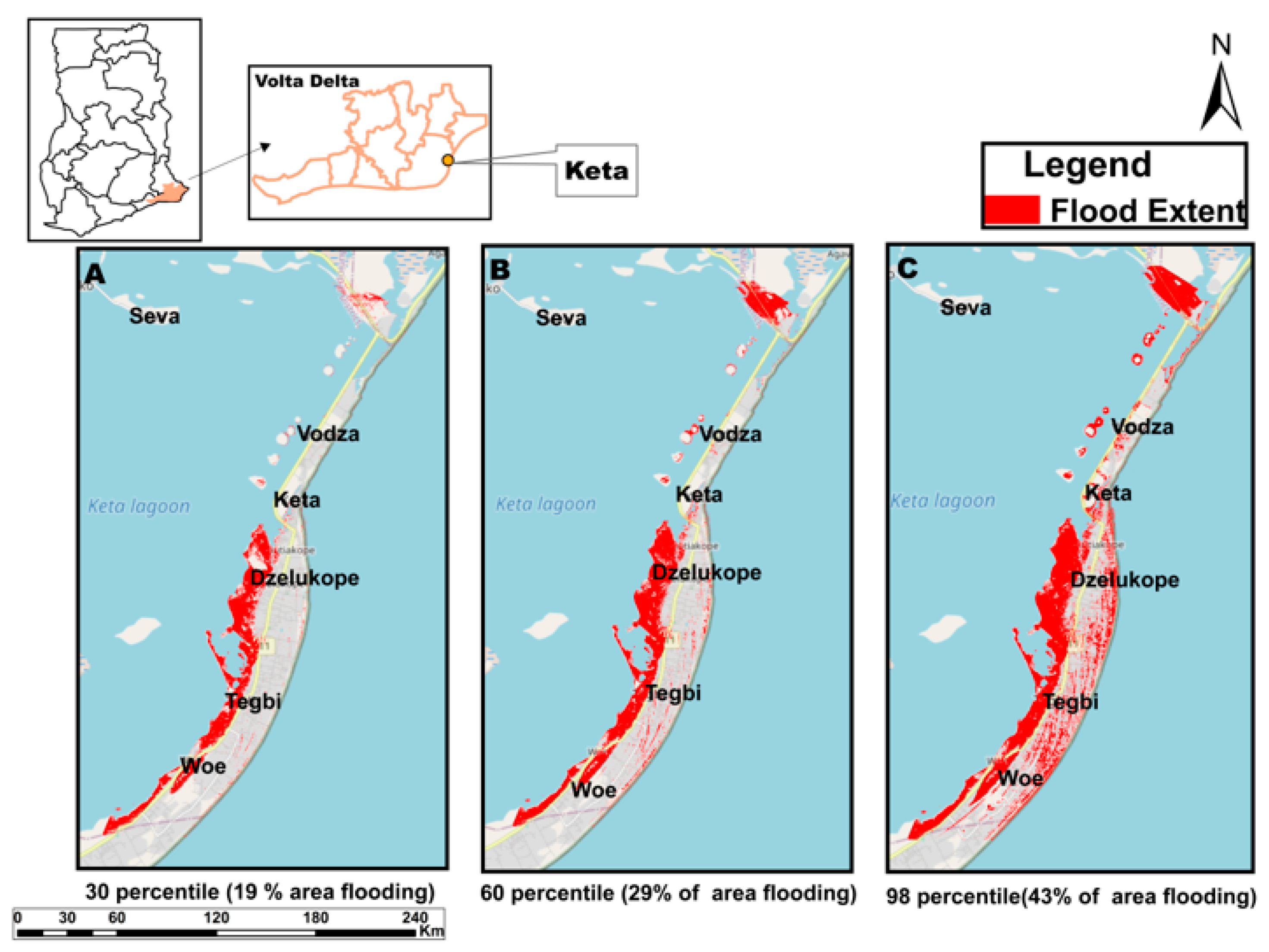
3.1. Percentile of Coastal Flood Occurrences

All ECWLs were ranked 30th, 60th, and 98th percentiles, corresponding to 0.54 m, 0.97 m, and 1.62 m, respectively. For example, from Figure 4, flood events obtained from the National Disaster Management Organization (NADMO) in the Keta District occurred around the 98th percentile (1.62 m).

3.2. Time Spent on 98th Percentile

Generally, for the 98th percentile, the maximum time spent on coastal flooding is 200 h per year. However, there is an increase in time spent from 1994 to 2015. Figure 5 shows a gradual increase in hours spent every year.

3.3. In-Situ Flood Occurrence Data

All data obtained from NADMO show that coastal flooding usually occurs from June to September (Table 1). July represents the most dominant month of coastal flooding between 2002 and 2015. While June is the least month of flood occurrence.

3.4. Flood Extent Mapping concerning Percentiles

Figure 6 shows the extent and percentage of potentially flooded areas for all percentiles. The highest percentage of the area flooded was recorded in the 98th percentile. The figure shows that 43% of the area would potentially flood. The 30th and 60th percentiles showed that 19% and 29% of the area would potentially be flooded, respectively. However, the most severe flooding is observed in the 98th percentile scenario.

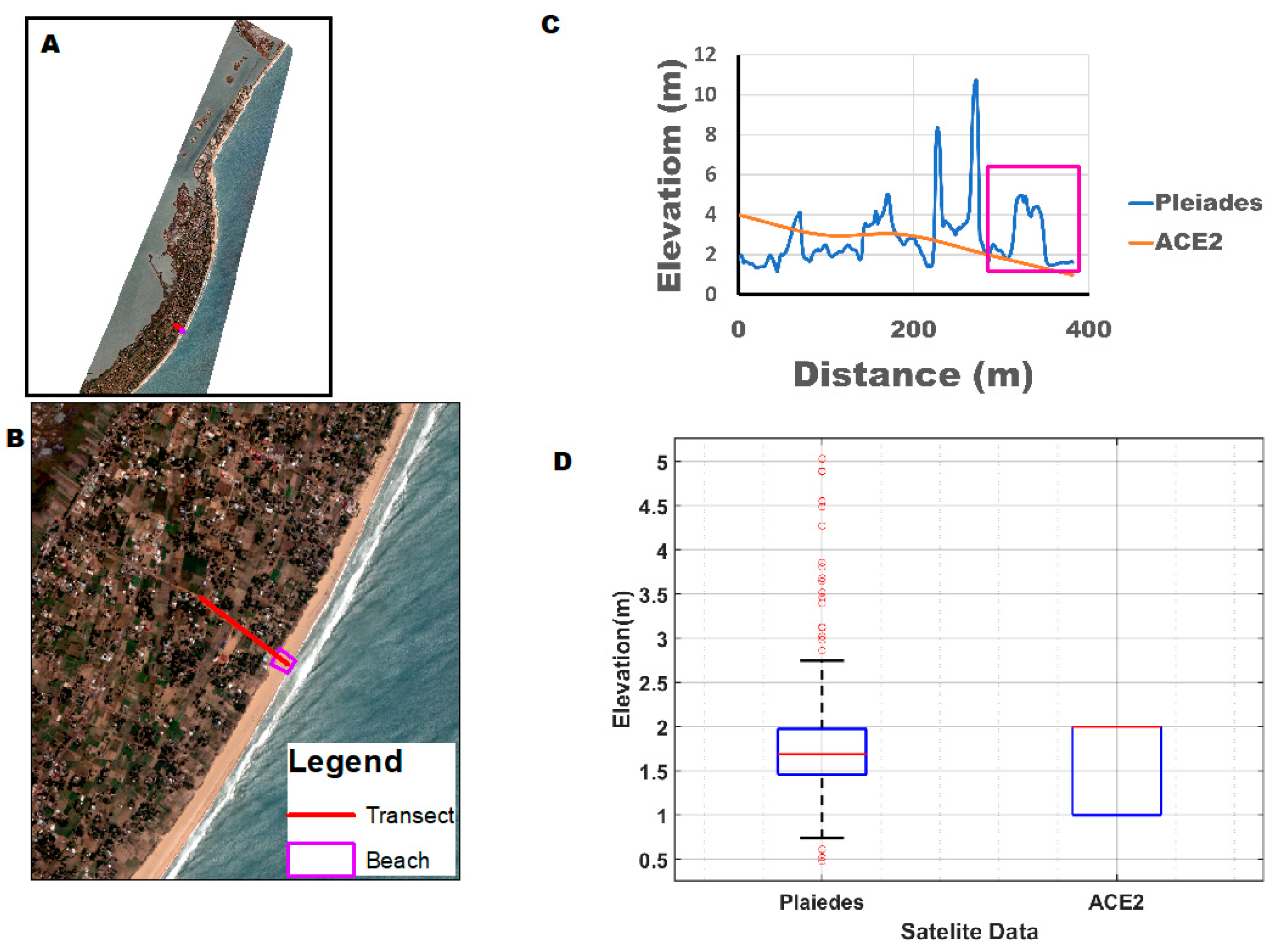
3.5. Comparison of Pleiades DEM and ACE2 DEM

A simple comparison between the two DEMs was assessed to show the ability of Pleiades DEMs to capture beach evolution and coastal flooding. Figure 7A and B show the location of the transect (red line) from which elevation profiles were extracted for both Pleiades and ACE2 DEMs. Figure 7C exhibits profile variations extracted for a distance of about 600 m, and this further shows a maximum elevation of 11 m high for Pleiades DEM and 2 m high for ACE2 DEM. This shows a very suitable representation and variation in the beach’s topography. Figure 7D is a box plot showing the variation and distribution of elevation along the transect. While Pleiades DEM shows a suitable elevation distribution and variation, ACE2 DEM barely shows any variation distribution in elevation within the same transect.

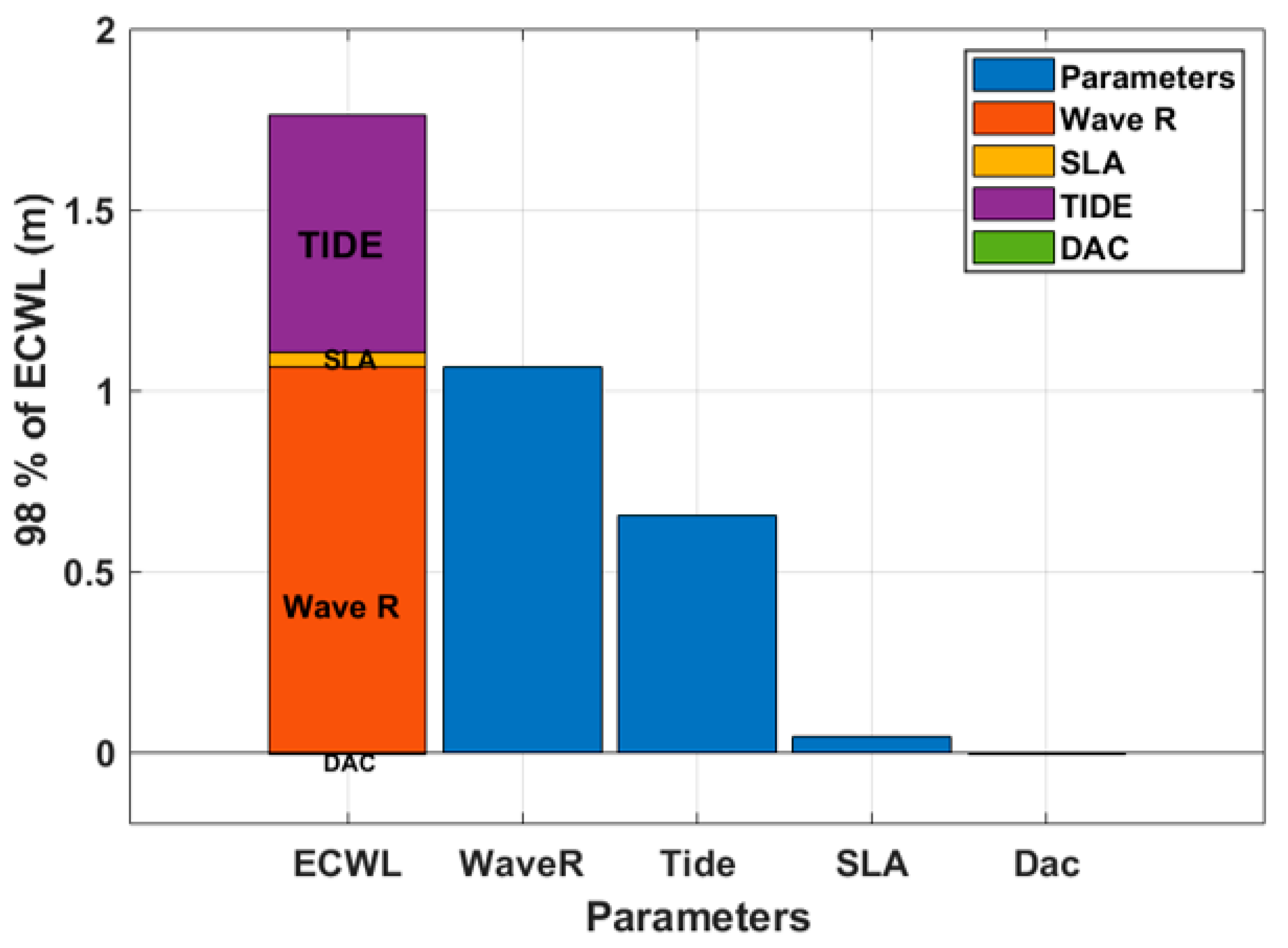
3.6. Hydrodynamic Contributors of Coastal Flooding

The major factors contributing to coastal flooding in the 98th percentile was evaluated from 1994 to 2015. Figure 8 shows the distribution of dominant factors in the ECWL. Waves have the highest contribution of 1.2 m compared to all other factors. Tide is the second highest contributor with 0.6 m, followed by SLA and DACs. Figure 8 shows that wave run-up dominates 98% of ECWLs to coastal flooding, followed by the tides, SLA, and DACs.

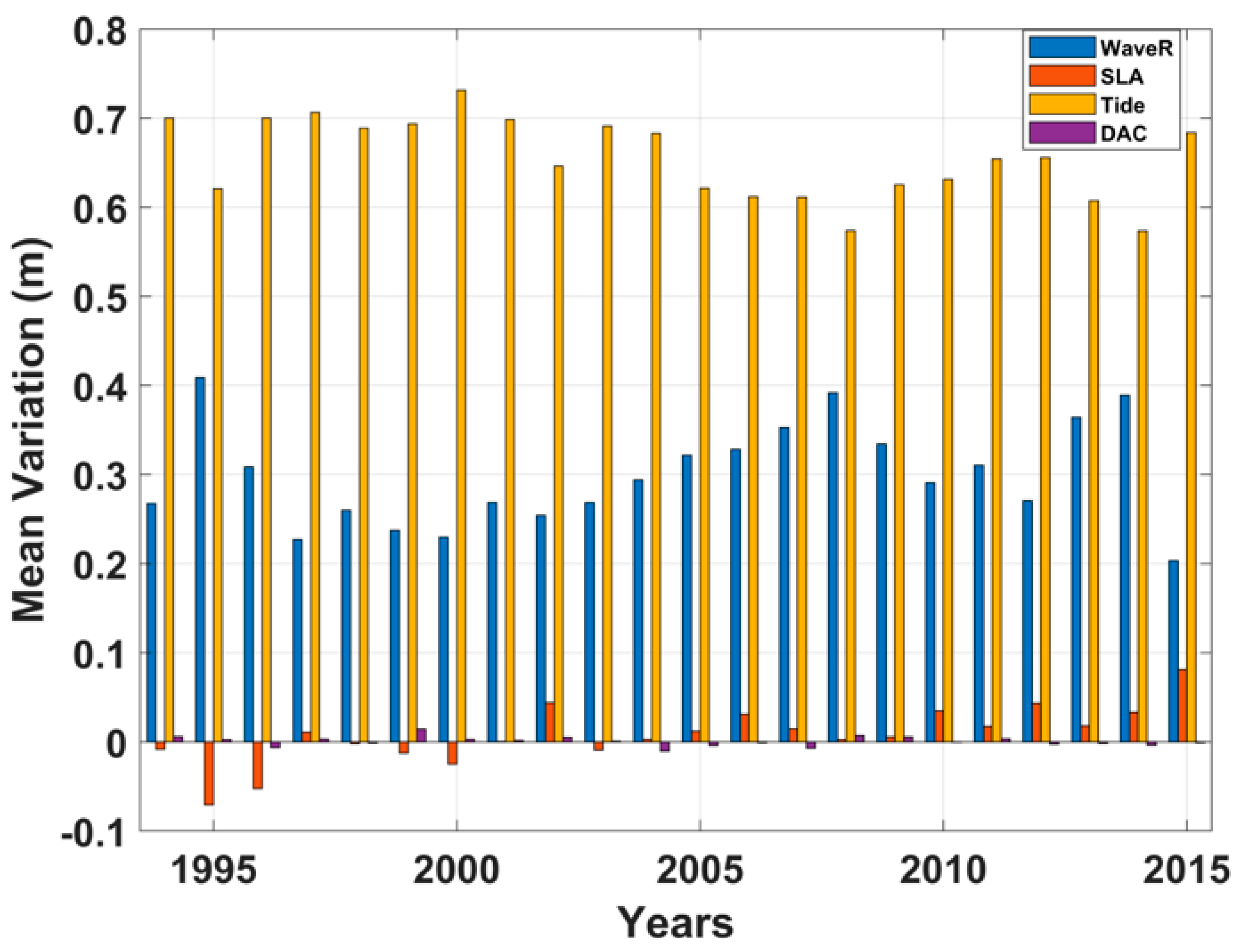
3.7. Variability of ECWL Parameters

Figure 9 shows the variability of parameters in 98% of ECWLs. A mean deviation plot was plotted to assess the variability between each parameter. From Figure 9, tide shows the highest variability among all the parameters, with about 0.75 m of variation. Though wave dominates from Figure 8, tides vary greatly during coastal flooding of 98% of ECWLs. On the other hand, parameters such as SLA and DACs exhibit very low variability between −0.05 and 0.05 m.

4. Discussion

Generally, low-lying regions experience coastal flooding. The findings of this study indicate that even with the smallest level of extreme coastal water levels (ECWLs), coastal flooding occurs. This phenomenon is common in low-lying areas such as deltas. Coastal flooding due to ECWLs can result from a single factor or a compound effect from several factors. On average, the Volta Delta experiences frequent flooding events (Figure 10) [32]. Most of these events have been attributed to “tidal waves”. However, as global warming increases extreme sea levels in the coming decades, coastal flooding is expected to become more frequent [57]. To understand which parameter contributes the most to extreme coastal events, all ECWLs were aggregated into severity ranks where the 98th percentile is the most severe, the 60th percentile is severe, and the 30th percentile is less severe. This study shows that all coastal flooding events in Keta District are in the 98th percentile of coastal flooding. This further indicates that coastal flooding in the Keta area was reported as a severe event from 2002 to 2015. ECWLs can result from a single ocean factor such as high tide, wave, or SLA. However, combining all these factors makes the scenario worse and more extreme. Coastal flooding at a given location occurs at varying temporal and spatial scales. This study shows that over the years, there has generally been an increase in the time spent by ECWLs. From Figure 5, the time spent by ECWLs reaches values as high as 200 hrs/year. This is consistent with the general sentiment of coastal flooding in the Volta Delta of Ghana over the past decade. In addition, global warming is still on the rise and thus accounts for the increase in flooding events and time spent per year during the most extreme events.
The spatial extent of coastal flooding by ECWLs shows that most of the area is potentially flooded in the 98th percentile of coastal flooding. Interestingly, in the 98th percentile case, parts of the main road and houses would potentially flood in the most extreme case. This is because the area is generally low-lying, and any minute increase in ECWLs would result in coastal flooding. The annual number of hours shows a positive (i.e., increasing) trend (calculated using the hourly ECWL time series for all years) (Figure 5.). The highest increase rates were observed in the 98th percentile and 2015. This is possible because coastal areas generally have low ECWL variability (time series variance). Thus, even a small increase in regional sea level can greatly impact coastal flooding [58]. ECWLs at the coast results from various, sometimes unrelated contributions, i.e., both natural and anthropogenic [59]. These include tides, meteorological processes, wave conditions, and sea level anomalies. Assessing the combination of these factors helps reduce the risk posed by coastal flooding [60].
For this reason, many global studies have attributed the cause of coastal flooding to sea level rise without considering the role of other factors along the coast [61,62,63,64]. This factor is equally important, as knowing about it would reduce the magnitude and exposure of physical damage. Appropriate planning and mitigation measures can be implemented with proper forecasting of extreme coastal events and a better understanding of the major contributors to coastal flooding at the local scale [65,66]. It is, however, worth knowing that, from Figure 7, Pleiades DEM can capture enough beach variations, such as the back beach, berm, and nearshore topography, compared to global DEM. This is relevant for coastal flooding studies since beach topography is very important for coastal flood prediction and how coastal structures impact and protect beaches.
Furthermore, in this study, wave run-up is the primary contributor to ECWLs for the Keta area. This confirms studies indicating that the Volta Delta is primarily wave-dominated, and thus all beaches are primarily formed and affected by wave activity [66,67]. In this study, the ECWLs at the 98th percentile have the wave run-up contributing as much as 70% to them (see Figure 8). In general, in the swash zone, single waves propagate beyond the slope of the beach and shoreline [68,69]. This area experiences significant erosion and wave overtopping during storms, as seen in Figure 10C. Water continuously covers and uncovers this area (Figure 10B). In particular, during a strong storm surge, waves affect the barrier beach or foredune more [70]. This also confirms the study by [18], which indicates that coastal flooding occurrences are expected to increase significantly in the coming decades.
For this reason, as the sea level rises, the study results show that considering wave contributions to long-term changes in total water level at the coast would lead to more accurate decadal forecasts and longer-term projections of total water level at the coast. Figure 9 shows the variability of the contributors in the ECWL. The tide is more variable on all time scales. Normally, the tide varies, including diurnal, biweekly with spring and neap tides, and seasonal and interannual scales. This explains why the tide is the most variable parameter among all parameters despite the predominance of waves in Figure 8. However, it is impossible to predict the phase between the tide and the wave run-up, which depend on independent factors. Overall, this increases the uncertainty of both short-term deterministic forecasts [17], while the probabilistic approach is more suitable for long-term prediction of overtopping and flooding [71]. Other factors, such as SLA and DACs, contribute to ECWLs, but their effects are rarely seen in the ECWLs. Using the Pleiades-derived DEM has proven to show how promising the Pleiades would contribute to studies in the coastal environment compared to global DEMs. This would be very helpful locally, particularly for coastal managers and engineers. Although operational accuracy without a ground control point is not yet possible for coastal studies at this stage (as stated by [22,35,72]), the limitations in accuracy encountered suggest that satellite-based topography monitoring can be a significant advancement in overcoming long-standing technological barriers in monitoring, thereby supporting local coastal engineering and coastal monitoring. By offering local perspectives, this study offers valuable insights for developing evidence-based measures to minimize damage and injury. As a result, using ECWLs will attract considerable attention from diverse audiences in West Africa, including researchers, practitioners, decision makers, and policymakers from various fields such as catchment management, engineering, economics, disaster management, and science-informed policy planning.

5. Conclusions

This study quantified coastal flooding from 1994 to 2015 in the historical city of Keta in the Volta Delta, Ghana. High-resolution coastal topography derived from Pleiades satellites and extreme coastal water levels (ECWLs), including wave contribution, were used to map potential flood areas. During the most severe situation (98% percentile of ECWLs), 43% of the Keta area is potentially flooded, including roads and inhabitants’ houses. The major hydrodynamic contributor to coastal flooding is wave run-up, which differs from Senegal, where tide dominates. On the other hand, while wave run-up dominates, the tide is more variable, indicating the key role of the phasing between components. The time spent (hrs/year) with potential severe flooding from 1994 to 2015 is increasing due to global mean sea level rise, as observed by satellite altimetry. It will most likely accelerate over the twentieth century with more and more people being displaced. Our local findings can help decrease exposure to damage and injury by developing pertinent science-based protection and mitigation solutions.

Author Contributions

Conceptualization, E.K.B. and R.A.; methodology, R.A. and E.K.B.; validation, E.K.B.; formal analysis, E.K.B.; investigation, data curation, E.K.B., R.A. and D.B.A.; writing—original draft preparation; E.K.B.; writing—review and editing, E.K.B., R.A., D.B.A., P.-N.J.-Q., K.T.A.-A. and B.C.; supervision, R.A., D.B.A. and P.A.D.M. All authors have read and agreed to the published version of the manuscript.

Funding

This research was funded by the Africa Centre of Excellence in Coastal Resilience (ACECoR), University of Cape Coast, with support from the World Bank and the Government of Ghana, World Bank ACE Grant Number is credit number 6389-G and Institute of Research Development coast under control project (IRD/JEAI) and the ACE PARTNER project of IRD.

Institutional Review Board Statement

Not applicable.

Informed Consent Statement

Not applicable.

Data Availability Statement

Not applicable.

Acknowledgments

This paper is part of a Ph.D. thesis under the Africa Centre of Excellence in Coastal Resilience (ACECoR), the University of Cape Coast, with the support of the World Bank and the Government of Ghana.

Conflicts of Interest

The authors declare no conflict of interest.

References

  1. Braun, A. Retrieval of digital elevation models from Sentinel-1 radar data—Open applications, techniques, and limitations. Open Geosci. 2021, 13, 532–569. [Google Scholar] [CrossRef]
  2. McGranahan, G.; Balk, D.; Anderson, B. The rising tide: Assessing the risks of climate change and human settlements in low elevation coastal zones. Environ. Urban. 2007, 19, 17–37. [Google Scholar] [CrossRef]
  3. Peter Sheng, Y.; Paramygin, V.A.; Yang, K.; Rivera-Nieves, A.A. A sensitivity study of rising compound coastal inundation over large flood plains in a changing climate. Sci. Rep. 2022, 12, 3403. [Google Scholar] [CrossRef] [PubMed]
  4. Dada, O.; Almar, R.; Morand, P.; Menard, F. Towards West African coastal social-ecosystems sustainability: Interdisciplinary approaches. Ocean Coast. Manag. 2021, 211, 105746. [Google Scholar] [CrossRef]
  5. Vousdoukas, M.I.; Clarke, J.; Ranasinghe, R.; Reimann, L.; Khalaf, N.; Duong, T.M.; Ouweneel, B.; Sabour, S.; Iles, C.E.; Trisos, C.H.; et al. African heritage sites threatened as sea-level rise accelerates. Nat. Clim. Chang. 2022, 12, 256–262. [Google Scholar] [CrossRef]
  6. Marcos, M.; Rohmer, J.; Vousdoukas, M.I.; Mentaschi, L.; Le Cozannet, G.; Amores, A. Increased Extreme Coastal Water Levels Due to the Combined Action of Storm Surges and Wind Waves. Geophys. Res. Lett. 2019, 46, 4356–4364. [Google Scholar] [CrossRef]
  7. Olbert, A.I.; Moradian, S.; Nash, S.; Comer, J.; Kazmierczak, B.; Falconer, R.A.; Hartnett, M. Combined statistical and hydrodynamic modelling of compound flooding in coastal areas—Methodology and application. J. Hydrol. 2023, 620, 129383. [Google Scholar] [CrossRef]
  8. Wahl, T.; Mudersbach, C.; Jensen, J. Assessing the hydrodynamic boundary conditions for risk analyses in coastal areas: A multivariate statistical approach based on Copula functions. Nat. Hazards Earth Syst. Sci. 2012, 12, 495–510. [Google Scholar] [CrossRef]
  9. Bilskie, M.V.; Hagen, S.C. Defining Flood Zone Transitions in Low-Gradient Coastal Regions. Geophys. Res. Lett. 2018, 45, 2761–2770. [Google Scholar] [CrossRef]
  10. Paprotny, D.; Vousdoukas, M.I.; Morales-Nápoles, O.; Jonkman, S.N.; Feyen, L. Compound flood potential in Europe. Hydrol. Earth Syst. Sci. Discuss. 2018, preprint. [Google Scholar] [CrossRef]
  11. Almar, R.; Ranasinghe, R.; Bergsma, E.W.J.; Diaz, H.; Melet, A.; Papa, F.; Vousdoukas, M.; Athanasiou, P.; Dada, O.; Almeida, L.P.; et al. A global analysis of extreme coastal water levels with implications for potential coastal overtopping. Nat. Commun. 2021, 12, 3775. [Google Scholar] [CrossRef]
  12. Nerem, R.S.; Beckley, B.D.; Fasullo, J.T.; Hamlington, B.D.; Masters, D.; Mitchum, G.T. Climate-change–driven accelerated sea-level rise detected in the altimeter era. Proc. Natl. Acad. Sci. USA 2018, 115, 2022–2025. [Google Scholar] [CrossRef] [PubMed]
  13. Church, J.A.; Clark, P.U.; Cazenave, A.; Gregory, J.M.; Jevrejeva, S.; Levermann, A.; Merrifield, M.A.; Milne, G.A.; Nerem, R.S.; Nunn, P.D.; et al. Sea-Level Rise by 2100. Science 2013, 342, 1445. [Google Scholar] [CrossRef] [PubMed]
  14. Gregory, J.M.; Griffies, S.M.; Hughes, C.W.; Lowe, J.A.; Church, J.A.; Fukimori, I.; Gomez, N.; Kopp, R.E.; Landerer, F.; Cozannet, G.L.; et al. Concepts and Terminology for Sea Level: Mean, Variability and Change, Both Local and Global. Surv. Geophys. 2019, 40, 1251–1289. [Google Scholar] [CrossRef]
  15. De Moel, H.; Jongman, B.; Kreibich, H.; Merz, B.; Penning-Rowsell, E.; Ward, P.J. Flood risk assessments at different spatial scales. Mitig. Adapt. Strat. Glob. Chang. 2015, 20, 865–890. [Google Scholar] [CrossRef]
  16. Van der Meer, J.; Nieuwenhuis, J.-W.; Steendam, G.J.; Reneerkens, M.; Steetzel, H.; van Vledder, G. Wave Overtopping Measurements at a Real Dike. Coast. Struct. 2019, 2019, 1107–1117. [Google Scholar] [CrossRef]
  17. Bertin, X.; Li, K.; Roland, A.; Zhang, Y.J.; Breilh, J.F.; Chaumillon, E. A modeling-based analysis of the flooding associated with Xynthia, central Bay of Biscay. Coast. Eng. 2014, 94, 80–89. [Google Scholar] [CrossRef]
  18. Melet, A.; Meyssignac, B.; Almar, R.; Le Cozannet, G. Under-estimated wave contribution to coastal sea-level rise. Nat. Clim. Chang. 2018, 8, 234–239. [Google Scholar] [CrossRef]
  19. Angnuureng, D.B.; Appeaning Addo, K.; Almar, R.; Dieng, H. Influence of sea level variability on a micro-tidal beach. Nat. Hazards 2018, 93, 1611–1628. [Google Scholar] [CrossRef]
  20. Vaze, J.; Teng, J.; Spencer, G. Impact of DEM accuracy and resolution on topographic indices. Environ. Model. Softw. 2010, 25, 1086–1098. [Google Scholar] [CrossRef]
  21. Almeida, L.; Almar, R.; Bergsma, E.; Berthier, E.; Baptista, P.; Garel, E.; Dada, O.; Alves, B. Deriving High Spatial-Resolution Coastal Topography From Sub-meter Satellite Stereo Imagery. Remote Sens. 2019, 11, 590. [Google Scholar] [CrossRef]
  22. Taveneau, A.; Almar, R.; Bergsma, E.W.J.; Sy, B.A.; Ndour, A.; Sadio, M.; Garlan, T. Observing and Predicting Coastal Erosion at the Langue de Barbarie Sand Spit around Saint Louis (Senegal, West Africa) through Satellite-Derived Digital Elevation Model and Shoreline. Remote Sens. 2021, 13, 2454. [Google Scholar] [CrossRef]
  23. Appeaning Addo, K.; Jayson-Quashigah, P.-N.; Codjoe, S.N.A.; Martey, F. Drone as a tool for coastal flood monitoring in the Volta Delta, Ghana. Geoenviron. Disasters 2018, 5, 17. [Google Scholar] [CrossRef]
  24. Bokpe, S. Azizanya is drowning 2010. Available online: http://sethbnews09.blogspot.com/2010/08/helpazizanya-is-drowning-friday-august.html (accessed on 23 April 2023).
  25. Matteo, F. West Africa is being swallowed by the sea. October 2016. Available online: http://foreignpolicy.com/2016/10/21/west-africa-is-being-swallowed-by-the-seaclimate-change-ghana-benin (accessed on 23 April 2023).
  26. Anthony, E.J. Patterns of Sand Spit Development and Their Management Implications on Deltaic, Drift-Aligned Coasts: The Cases of the Senegal and Volta River Delta Spits, West Africa. In Sand and Gravel Spits; Randazzo, G., Jackson, D.W.T., Cooper, J.A.G., Eds.; Coastal Research Library; Springer International Publishing: Cham, Switzerland, 2015; Volume 12, pp. 21–36. ISBN 978-3-319-13715-5. [Google Scholar]
  27. Appeaning Addo, K.; Brempong, E.K.; Jayson-Quashigah, P.N. Assessment of the dynamics of the Volta river estuary shorelines in Ghana. Geoenviron. Disasters 2020, 7, 19. [Google Scholar] [CrossRef]
  28. Ly, C.K. The role of the Akosombo Dam on the Volta river in causing coastal erosion in central and eastern Ghana (West Africa). Mar. Geol. 1980, 37, 323–332. [Google Scholar] [CrossRef]
  29. Akpati, B.N. Geologic structure and evolution of the Keta basin, Ghana, West Africa. Geol. Soc. Am. Bull. 1978, 89, 124. [Google Scholar] [CrossRef]
  30. Kabo-bah, A.; Diji, C.J. (Eds.) Sustainable Hydropower in West Africa: Planning, Operation, and Challenges; Academic Press, an imprint of Elsevier: London, UK; San Diego, CA, USA, 2018; ISBN 978-0-12-813016-2. [Google Scholar]
  31. Garr, E. Infrastructure policy reforms and rural poverty reduction in Ghana: The case of the Keta Sea Defence Project, University of the Western Cape. 2010. Available online: https://core.ac.uk/download/pdf/58913725.pdf (accessed on 23 April 2023).
  32. Addo, K.A.; Nicholls, R.J.; Codjoe, S.N.A.; Abu, M. A Biophysical and Socioeconomic Review of the Volta Delta, Ghana. J. Coast. Res. 2018, 345, 1216–1226. [Google Scholar] [CrossRef]
  33. Roest, L.W.M. The coastal system of the Volta delta, Ghana Opportunities and strategies for development. Available online: https://pure.tudelft.nl/ws/files/37464456/Roest_2018_The_coastal_system_of_the_Volta_delta.pdf (accessed on 20 March 2023).
  34. Duku, E.; Dzorgbe Mattah, P.A.; Angnuureng, D.B. Assessment of wetland ecosystem services and human wellbeing nexus in sub-Saharan Africa: Empirical evidence from a socio-ecological landscape of Ghana. Environ. Sustain. Indic. 2022, 15, 100186. [Google Scholar] [CrossRef]
  35. Turner, I.L.; Harley, M.D.; Almar, R.; Bergsma, E.W.J. Satellite optical imagery in Coastal Engineering. Coast. Eng. 2021, 167, 103919. [Google Scholar] [CrossRef]
  36. Almar, R.; Bergsma, E.W.J.; Maisongrande, P.; de Almeida, L.P.M. Wave-derived coastal bathymetry from satellite video imagery: A showcase with Pleiades persistent mode. Remote Sens. Environ. 2019, 231, 111263. [Google Scholar] [CrossRef]
  37. Almar, R.; Stieglitz, T.; Addo, K.A.; Ba, K.; Ondoa, G.A.; Bergsma, E.W.J.; Bonou, F.; Dada, O.; Angnuureng, D.; Arino, O. Coastal Zone Changes in West Africa: Challenges and Opportunities for Satellite Earth Observations. Surv. Geophys. 2023, 44, 249–275. [Google Scholar] [CrossRef]
  38. Gleyzes, M.A.; Perret, L.; Kubik, P. Pleiades system architecture and main performances. Int. Arch. Photogramm. Remote Sens. Spat. Inf. Sci. 2012, XXXIX-B1, 537–542. [Google Scholar] [CrossRef]
  39. Jacobsen, K.; Topan, H. Corrigendum to “DEM Generation with short base length pleiades triplet”. Int. Arch. Photogramm. Remote Sens. Spat. Inf. Sci. 2015, XL-3/W2, 297. [Google Scholar] [CrossRef]
  40. Carrere, L.; Lyard, F.; Cancet, M.; Guillot, A. FES 2014, a new tidal model on the global ocean with enhanced accuracy in shallow seas and in the Arctic region. In Proceedings of the EGU General Assembly, Vienna, Austria, 12–17 April 2015. [Google Scholar]
  41. Soudarin, L.; Rosmordu, V.; Guinle, T.; Nino, F.; Birol, F.; Mertz, F.; Schgounn, C.; Gasc, M. Aviso+: Altimetry satellite data and products for ocean-oriented applications (and others). In Proceedings of the 20th EGU General Assembly, EGU2018, Vienna, Austria, 4–13 April 2018; p. 1608. [Google Scholar]
  42. Marti, F.; Cazenave, A.; Birol, F.; Passaro, M.; Léger, F.; Niño, F.; Almar, R.; Benveniste, J.; Legeais, J.F. Altimetry-based sea level trends along the coasts of Western Africa. Adv. Space Res. 2021, 68, 504–522. [Google Scholar] [CrossRef]
  43. Stockdon, H.F.; Holman, R.A.; Howd, P.A.; Sallenger, A.H. Empirical parameterization of setup, swash, and runup. Coast. Eng. 2006, 53, 573–588. [Google Scholar] [CrossRef]
  44. Rupnik, E.; Pierrot-Deseilligny, M.; Delorme, A. 3D reconstruction from multi-view VHR-satellite images in MicMac. ISPRS J. Photogramm. Remote Sens. 2018, 139, 201–211. [Google Scholar] [CrossRef]
  45. Palaseanu-Lovejoy, M.; Bisson, M.; Spinetti, C.; Buongiorno, M.F.; Alexandrov, O.; Cecere, T. High-Resolution and Accurate Topography Reconstruction of Mount Etna from Pleiades Satellite Data. Remote Sens. 2019, 11, 2983. [Google Scholar] [CrossRef]
  46. Shean, D.E.; Alexandrov, O.; Moratto, Z.M.; Smith, B.E.; Joughin, I.R.; Porter, C.; Morin, P. An automated, open-source pipeline for mass production of digital elevation models (DEMs) from very-high-resolution commercial stereo satellite imagery. ISPRS J. Photogramm. Remote Sens. 2016, 116, 101–117. [Google Scholar] [CrossRef]
  47. Facciolo, G.; Franchis, C.D.; Meinhardt, E. MGM: A Significantly More Global Matching for Stereovision. In Proceedings of the British Machine Vision Conference 2015, Swansea, UK, 7–10 September 2015; pp. 90.1–90.12. [Google Scholar]
  48. Knuth, F.; Shean, D.; Bhushan, S.; Schwat, E.; Alexandrov, O.; McNeil, C.; Dehecq, A.; Florentine, C.; O’Neel, S. Historical Structure from Motion (HSfM): Automated processing of historical aerial photographs for long-term topographic change analysis. Remote Sens. Environ. 2023, 285, 113379. [Google Scholar] [CrossRef]
  49. Jayson-Quashigah, P.-N.; Appeaning Addo, K.; Amisigo, B.; Wiafe, G. Assessment of short-term beach sediment change in the Volta Delta coast in Ghana using data from Unmanned Aerial Vehicles (Drone). Ocean Coast. Manag. 2019, 182, 104952. [Google Scholar] [CrossRef]
  50. Mesa-Mingorance, J.L.; Ariza-López, F.J. Accuracy Assessment of Digital Elevation Models (DEMs): A Critical Review of Practices of the Past Three Decades. Remote Sens. 2020, 12, 2630. [Google Scholar] [CrossRef]
  51. Collilieux, X.; Wöppelmann, G. Global sea-level rise and its relation to the terrestrial reference frame. J. Geod. 2011, 85, 9–22. [Google Scholar] [CrossRef]
  52. Yunus, A.; Avtar, R.; Kraines, S.; Yamamuro, M.; Lindberg, F.; Grimmond, C. Uncertainties in Tidally Adjusted Estimates of Sea Level Rise Flooding (Bathtub Model) for the Greater London. Remote Sens. 2016, 8, 366. [Google Scholar] [CrossRef]
  53. Leal-Alves, D.C.; Weschenfelder, J.; Albuquerque, M.d.G.; Espinoza, J.M. de A.; Ferreira-Cravo, M.; Almeida, L.P.M. de Digital elevation model generation using UAV-SfM photogrammetry techniques to map sea-level rise scenarios at Cassino Beach, Brazil. SN Appl. Sci. 2020, 2, 2181. [Google Scholar] [CrossRef]
  54. Didier, D.; Baudry, J.; Bernatchez, P.; Dumont, D.; Sadegh, M.; Bismuth, E.; Bandet, M.; Dugas, S.; Sévigny, C. Multihazard simulation for coastal flood mapping: Bathtub versus numerical modelling in an open estuary, Eastern Canada. J. Flood Risk Manag. 2019, 12, e12505. [Google Scholar] [CrossRef]
  55. Rizzo, A.; Vandelli, V.; Gauci, C.; Buhagiar, G.; Micallef, A.S.; Soldati, M. Potential Sea Level Rise Inundation in the Mediterranean: From Susceptibility Assessment to Risk Scenarios for Policy Action. Water 2022, 14, 416. [Google Scholar] [CrossRef]
  56. Snoussi, M.; Ouchani, T.; Niazi, S. Vulnerability assessment of the impact of sea-level rise and flooding on the Moroccan coast: The case of the Mediterranean eastern zone. Estuar. Coast. Shelf Sci. 2008, 77, 206–213. [Google Scholar] [CrossRef]
  57. Walsh, K.J.E.; McInnes, K.L.; McBride, J.L. Climate change impacts on tropical cyclones and extreme sea levels in the South Pacific—A regional assessment. Glob. Planet. Chang. 2012, 80–81, 149–164. [Google Scholar] [CrossRef]
  58. Taherkhani, M.; Vitousek, S.; Barnard, P.L.; Frazer, N.; Anderson, T.R.; Fletcher, C.H. Sea-level rise exponentially increases coastal flood frequency. Sci. Rep. 2020, 10, 6466. [Google Scholar] [CrossRef]
  59. Woodworth, P.L.; Melet, A.; Marcos, M.; Ray, R.D.; Wöppelmann, G.; Sasaki, Y.N.; Cirano, M.; Hibbert, A.; Huthnance, J.M.; Monserrat, S.; et al. Forcing Factors Affecting Sea Level Changes at the Coast. Surv. Geophys. 2019, 40, 1351–1397. [Google Scholar] [CrossRef]
  60. Imani, M.; Kuo, C.-Y.; Chen, P.-C.; Tseng, K.-H.; Kao, H.-C.; Lee, C.-M.; Lan, W.-H. Risk Assessment of Coastal Flooding under Different Inundation Situations in Southwest of Taiwan (Tainan City). Water 2021, 13, 880. [Google Scholar] [CrossRef]
  61. Amores, A.; Marcos, M.; Pedreros, R.; Le Cozannet, G.; Lecacheux, S.; Rohmer, J.; Hinkel, J.; Gussmann, G.; Van Der Pol, T.; Shareef, A.; et al. Coastal Flooding in the Maldives Induced by Mean Sea-Level Rise and Wind-Waves: From Global to Local Coastal Modelling. Front. Mar. Sci. 2021, 8, 665672. [Google Scholar] [CrossRef]
  62. Mimura, N. Sea-level rise caused by climate change and its implications for society. Proc. Jpn. Acad. Ser. B 2013, 89, 281–301. [Google Scholar] [CrossRef]
  63. Nicholls, R.J. Analysis of global impacts of sea-level rise: A case study of flooding. Phys. Chem. Earth Parts A/B/C 2002, 27, 1455–1466. [Google Scholar] [CrossRef]
  64. Nicholls, R.J.; Tol, R.S.J. Impacts and responses to sea-level rise: A global analysis of the SRES scenarios over the twenty-first century. Phil. Trans. R. Soc. A. 2006, 364, 1073–1095. [Google Scholar] [CrossRef] [PubMed]
  65. Ciavola, P.; Ferreira, O.; Haerens, P.; Van Koningsveld, M.; Armaroli, C. Storm impacts along European coastlines. Part 2: Lessons learned from the MICORE project. Environ. Sci. Policy 2011, 14, 924–933. [Google Scholar] [CrossRef]
  66. Anthony, E.J.; Orford, J.D. Between Wave- and Tide-Dominated Coasts: The Middle Ground Revisited. J. Coast. Res. 2002, 36, 8–15. [Google Scholar] [CrossRef]
  67. Jayson-Quashigah, P.-N.; Appeaning Addo, K.; Wiafe, G.; Amisigo, B.A.; Brempong, E.K.; Kay, S.; Angnuureng, D.B. Wave dynamics and shoreline evolution in deltas: A case study of sandy coasts in the Volta delta of Ghana. Interpretation 2021, 9, SH99–SH113. [Google Scholar] [CrossRef]
  68. Deng, B.; Zhang, W.; Yao, Y.; Jiang, C. A laboratory study of the effect of varying beach slopes on bore-driven swash hydrodynamics. Front. Mar. Sci. 2022, 9, 956379. [Google Scholar] [CrossRef]
  69. Chen, W.; Van Der Werf, J.J.; Hulscher, S.J.M.H. A review of practical models of sand transport in the swash zone. Earth-Sci. Rev. 2023, 238, 104355. [Google Scholar] [CrossRef]
  70. Mehrtens, B.; Lojek, O.; Kosmalla, V.; Bölker, T.; Goseberg, N. Foredune growth and storm surge protection potential at the Eiderstedt Peninsula, Germany. Front. Mar. Sci. 2023, 9, 1020351. [Google Scholar] [CrossRef]
  71. Vousdoukas, M.I.; Mentaschi, L.; Voukouvalas, E.; Verlaan, M.; Jevrejeva, S.; Jackson, L.P.; Feyen, L. Global probabilistic projections of extreme sea levels show intensification of coastal flood hazard. Nat. Commun. 2018, 9, 2360. [Google Scholar] [CrossRef] [PubMed]
  72. Cisse, C.O.T.; Brempong, E.K.; Taveneau, A.; Almar, R.; Sy, B.A.; Angnuureng, D.B. Extreme coastal water levels with potential flooding risk at the low-lying Saint Louis historic city, Senegal (West Africa). Front. Mar. Sci. 2022, 9, 993644. [Google Scholar] [CrossRef]
Figure 1. A map of the study area showing (A) an image of Ghana with all districts and the Volta Delta shaded in yellow; (B) an image of the Volta Delta showing all the districts with the water bodies in the Volta Delta; and (C) an image of Keta District with Pleiades multi-spectral satellite image superimposed showing the major towns and tourist sites in the Keta District of the Volta Delta, Ghana (Gulf of Guinea, West Africa).
Jmse 11 01144 g001
Figure 2. An image of the tri-stereo images (PHR1A) acquired on 20 October 2020 for the Keta study area (made using Google Earth).
Jmse 11 01144 g002
Figure 3. A summary of the methodology for NASA’s Ames Stereo Pipeline software (ASP) for structure from motion procedure workflow implemented in this study. This approach derives DEMs and orthophotos from satellite imagery.
Jmse 11 01144 g003
Figure 4. A percentile distribution plot of extreme coastal water levels from 1994 to 2015 showing the 30th, 60th, and 98th percentile with occurrences of coastal flooding obtained from NADMO in blue dots.
Jmse 11 01144 g004
Figure 5. Time spent by an occurrence at the 98th percentile in hours per year from 1994 to 2015, showing blue dots of maximum annual ECWL data and red trend line from 1994 to 2015.
Jmse 11 01144 g005
Figure 6. Flood extent mapping for each scenario of ECWLs where: (A) 30th percentile of ECWLs with 19% of the area being potentially flooded, (B) 60th percentile of ECWLs with 29% of the area being potentially flooded, (C) 98th percentile of the area being potentially flooded.
Jmse 11 01144 g006
Figure 7. (A) An orthophoto of the Pleiades imagery for the Keta municipality with a red line. (B) The zoomed-in orthophoto of the selected transect and a purple box showing the beach area. (C) Elevation variation for Pleiades and ACE2 with a purple box showing the beach area of the transect. (D) A box plot of elevation along the transect shows the distribution of Pleiades and ACE2 imagery elevation values.
Jmse 11 01144 g007
Figure 8. Hydrodynamic contributors to coastal flooding at 98%, showing the contribution of all parameters in ECWLs at 98% of ECWLs. The extreme left shows a stack bar plot of all parameters, with wave R, tide, SLA, and DACs showing the dominance hierarchy, respectively. All plots in blue show varying levels of these parameters in the same hierarchy.
Jmse 11 01144 g008
Figure 9. Variation in contributors of ECWLs from 1994 to 2015 using the yearly mean deviation of all parameters for 98% of ECWLs from 1994 to 2015.
Jmse 11 01144 g009
Figure 10. The imagery of beach resorts affected by ECWLs; (A) an aerial view of two major beach resorts (Aborigines beach resort and Agblor Lodge) in Keta without flooding; (B) gradual flooding of the Agblor Lodge and Aborigines beach resort being affected by ECWLs; (C) an aerial view of wave overtopping in the Keta area due to ECWLs. (Photo A obtained from https://www.agblorlodge.com/gallery_cat/aerial-photograph/ (accessed on 21 April 2023); photo credit of B and C: Brempong Emmanuel).
Jmse 11 01144 g010
Table 1. The occurrence of coastal flooding was obtained from NADMO from 2002 to 2015. Generally, all data obtained from NADMO range between 2002 and 2015. There are no data available from 1994 to 2002. All data sets were collected by observing flooding and reporting by the NADMO office in Keta, Ghana.
Year of OccurrenceMonth of Occurrence
2002August
2003September
2004July
2005July
2006September
2007July
2008August
2009September
2010August
2011July
2012June
2013July
2014August
2015September
Disclaimer/Publisher’s Note: The statements, opinions and data contained in all publications are solely those of the individual author(s) and contributor(s) and not of MDPI and/or the editor(s). MDPI and/or the editor(s) disclaim responsibility for any injury to people or property resulting from any ideas, methods, instructions or products referred to in the content.

