Effects of Mud Supply and Hydrodynamic Conditions on the Sedimentary Distribution of Estuaries: Insights from Sediment Dynamic Numerical Simulation

Abstract

Estuaries are important sediment facies in the fluvial-to-marine transition zone, are strongly controlled by dynamic interactions of tides, waves, and fluvial flows, and show various changes in depositional processes and sediment distribution. Deep investigations on the sediment dynamic processes of the sand component of estuaries have been conducted; however, the understanding of how mud supply affects estuaries’ sedimentary characteristics and morphology is still in vague. Herein, the effects of mud concentration, mud transport properties, fluvial discharge, and tidal amplitude on the sedimentary characteristics of an estuary were systematically analyzed using sedimentary dynamic numerical simulation. The results show that the mud concentration has significant effects on the morphology of tidal channels in estuaries, which become more braided with a lower mud concentration, and straighter, with reduced channel migration, with a higher mud concentration. The mud transport properties, namely, setting velocity, critical bed shear stress for sedimentation, and erosion, mostly affect the ratio between the length and width (RLW) of the sand bar; a sheet-like sand bar with a lower RLW value develops in the lower settling velocity, while there are obvious strip shaped bars with a high RLW value in the higher settling velocity case. Moreover, the effects of hydrodynamic conditions on sedimentary distribution were analyzed by changing the tidal amplitudes and fluvial discharges. The results show that a higher tidal amplitude is often accompanied by a stronger tidal energy, which induces a more obvious seaward progradation, while a higher fluvial discharge usually yields a higher deposition rate and yields a greater deposition thickness. From the above numerical simulations, the statistical characteristics of tidal bars and mud interlayers were further obtained, which show good agreement with modern sedimentary characteristics. This study suggests that sedimentary dynamic numerical simulation can provide insights into an efficient quantitative method for analyzing the effects of mud components on the sediment processes of estuaries.

1. Introduction

The fluvial-to-marine transition zone is the area with the most complex sedimentary environments controlled by the continuous interaction of fluvial flows, tide currents, and waves [1,2,3,4]. Among which, estuaries are typical sediment systems [5,6], comprising predominantly sand components and minor mud components and salt marshes [7]. The interaction between mud and sand helps in promoting the long-term morphology of estuaries. Since the mud component has higher erosion resistance and lower sedimentary rate than the sand component [8,9], the mud layer can reduce the re-erosion of the underlying sand body and afford more stable sand bars and banks. Hence, the mud component might help in the dynamic balancing between sand body erosion and deposition in estuaries [10].

Recently, increasing attention has been paid to the sedimentary distribution and reservoir architecture of estuaries [11,12], and a series of works has been conducted on the main controlling factors of estuary sedimentation [13,14], such as fluvial discharge, slope angle, and wave. Winterwerp [15] believed that source supply direction is the main controlling factor in the location of mud deposits and hydrodynamic conditions are a secondary controlling factor. Verlaan [16] studied the mud distribution characteristics of different source supplies in estuaries and found that marine mud mainly settles in the entrance channels of lower estuaries, while relatively small amounts are deposited further upstream. Conversely, fluvial mud is mainly deposited in the inner estuary. Cleveringa and Dam [17] implied that hydrodynamic conditions have significant affects on the locations of mudflats, as mudflats exhibit a faster migration with rapid changes in flood-dominated peak velocities. Conversely, Kleinhans and M. [18] argued that the hydrodynamic conditions only change their scales instead of changing the location of mudflats. Schramkowski et al. [19] and Toffolon and Crosato [20] argued that hydrodynamic conditions are the major factor affecting the development of sand bars in an estuary. The length of sand bars is positively correlated with fluvial discharge and tidal range. Wave-generated currents are a third mechanism leading to sediment transport and sand bar morphodynamics [21]. The research show that waves mainly act on the shape of the estuary. Waves cause the estuary to widen and limit the deposition of mud. Although previous studies have provided a certain understanding on the sedimentary characteristics of estuaries and the factors affecting tidal bar development, there are several controversial points. Consequently, exploring the effects of mud supply and hydrodynamic conditions on the development mechanism of estuary sedimentation is necessary. Many research methods have been applied to estuary sediments, including sedimentary record analysis, modern sedimentary anatomy, physical simulation, and numerical simulation [22,23,24,25,26]. The lack of recorded information and the limitations of experimental operation have led to large errors in the experimental results of traditional research methods. Meanwhile, advances in computer technology have promoted the rapid development of sedimentary numerical simulation. Sedimentary dynamic numerical simulation has become the mainstream research method for investigating different hydrodynamic and sedimentary driving mechanisms [27,28], providing strong support for studying the morphological dynamics and stratigraphic patterns [7]. Weisscher et al. [29] published the use of the morphological dynamic model Nays2D to determine the impact of dynamic inflow disturbances on river patterns. Edmonds and Slingerland [30] argued the effect of flow velocity and sediment transport on the sedimentary body formation using sedimentary dynamic numerical simulation. van de Lageweg et al. [13] suggested that fluvial discharge and tidal amplitude have a functional relationship between mud-deposit coverage and mud-deposit thickness based on numerical simulation. Tang et al. [28] used numerical simulation to study the reservoir configuration of tidal-controlled estuaries. Hence, sedimentary numerical simulation is used to simulate the geomorphic evolution of estuaries, which provides a new idea for analyzing the characteristics of mud deposition [31].

Herein, sedimentary dynamic numerical simulation was used to set different mud supply and hydrodynamic conditions, perform the sedimentation simulation of the tidal bar and its interlayer, and explore the effects of the controlling factors on the sedimentary development and distribution of an estuary. Nine cases of an idealized estuary model were designed for identifying effect of the key factors, namely, mud concentration, mud transport properties, fluvial discharge, and tidal amplitude on the sedimentary characteristics of the estuary. This paper is arranged as follows. Section 2 introduces the simulation setting and numerical parameters, Section 3 shows the simulation results of nine scenarios, and Section 4 compares the numerical models and natural estuaries and discusses the length, thickness, and frequency distributions of mud interlayers in detail.

2. Method and Parameters

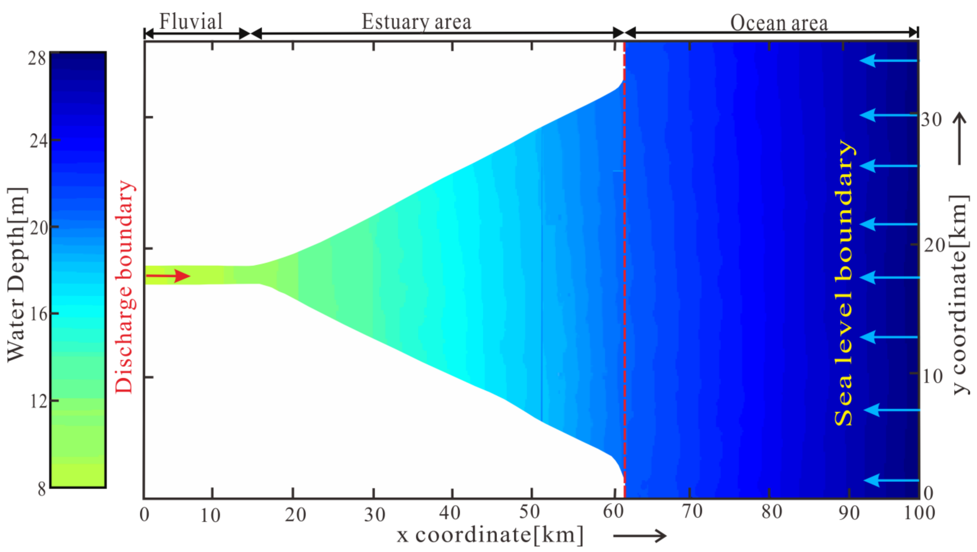
2.1. Numerical Simulation Method

The sedimentary processes in estuaries are simulated using the computational fluid dynamics software Delft3D [32], which uses numerical calculation methods to solve the Navier–Stokes equations and sediment transport based on an interleaved uniform finite-difference grid with the alternating direction implicit method. The flow module of Delft3D has been extensively applied to the study of topography and geomorphology in semi-enclosed coastal areas such as shallow seas, estuaries, and deltas [33,34,35,36]. The tidal–fluvial interaction of weakly forced stratified estuary systems is calculated using the momentum equations (Equations (1)–(3)).

$$\frac{\partial u}{\partial t}+\frac{u}{\sqrt{G_{\xi \xi }}}\frac{\partial u}{\partial \xi }+\frac{v}{\sqrt{G_{\eta \eta }}}\frac{\partial v}{\partial \eta }+\frac{w}{d+\zeta }\frac{\partial u}{\partial \sigma }-\frac{v^2}{\sqrt{G_{\xi \xi }}\sqrt{G_{\eta \eta }}}\frac{\partial \sqrt{G_{\eta \eta }}}{\partial \xi }+\frac{uv}{\sqrt{G_{\xi \xi }}\sqrt{G_{\eta \eta }}}\frac{\partial \sqrt{G_{\xi \xi }}}{\partial \eta }-fv=-\frac{1}{{\rho }_0\sqrt{G_{\xi \xi }}}{P}_{\xi }+F_{\xi }+\frac{1}{{\left(d+\zeta \right)}^2} \frac{\partial }{\partial \sigma }\left({\nu }_V\frac{\partial u}{\partial \sigma }\right)+M_{\xi }$$

(1)

$$\frac{\partial v}{\partial t}+\frac{u}{\sqrt{G_{\xi \xi }}}\frac{\partial v}{\partial \xi }+\frac{v}{\sqrt{G_{\eta \eta }}}\frac{\partial v}{\partial \eta }+\frac{w}{d+\zeta }\frac{\partial u}{\partial \sigma }+\frac{uv}{\sqrt{G_{\xi \xi }}\sqrt{G_{\eta \eta }}}\frac{\partial \sqrt{G_{\eta \eta }}}{\partial \xi }-\frac{u^2}{\sqrt{G_{\xi \xi }}\sqrt{G_{\eta \eta }}}\frac{\partial \sqrt{G_{\xi \xi }}}{\partial \eta }+fu=-\frac{1}{{\rho }_0\sqrt{G_{\eta \eta }}}{P}_{\eta }+F_{\eta }+\frac{1}{{\left(d+\zeta \right)}^2} \frac{\partial }{\partial \sigma }\left({\nu }_V\frac{\partial v}{\partial \sigma }\right)+M_{\eta }$$

(2)

$$\frac{\partial \zeta }{\partial t}+\frac{1}{\sqrt{G_{\xi \xi }}\sqrt{G_{\eta \eta }}}\frac{\partial \left(\left(d+\zeta \right)u\sqrt{G_{\eta \eta }}\right)}{\partial \xi }\frac{1}{\sqrt{G_{\xi \xi }}\sqrt{G_{\eta \eta }}}\frac{\partial \left(\left(d+\zeta \right)v\sqrt{G_{\eta \eta }}\right)}{\partial \eta }-\frac{\partial w}{\partial \sigma }=\left(d+\zeta \right) \left(q_{in}-q_{out}\right)$$

(3)

where $t$ is time (s), $\xi$ and $\eta$ are horizontal coordinates, $\sigma$ is the scaled vertical coordinate, $u$ is the flow velocity in the $\xi$-direction (ms⁻¹), $v$ is the fluid velocity in the $\eta$-direction (ms⁻¹), $w$ is the fluid velocity in the z-direction (ms⁻¹), $\zeta$ is the water level above some horizontal plane of reference (datum), $F_{\xi }$ and $F_{\eta }$ are turbulent momentum fluxes in the $\xi$ and $\eta$ directions (ms⁻²), $\sqrt{G_{\xi \xi }}$ and $\sqrt{G_{\eta \eta }}$ are coefficients used to transform the curvilinear to rectangular ones, $M_{\xi } \mathrm{and} M_{\eta }$ are the sources or sinks of momentum in the $\xi$ and $\eta$ directions (ms⁻²), $P_{\xi }$ and $P_{\eta }$ are gradient hydrostatic pressures in the $\xi$ and $\eta$ directions (kgm⁻²s⁻²), $f$ is the Coriolis parameter (s⁻¹), d is the depth below some horizontal plane of reference (datum), ${\nu }_V$ is the vertical eddy viscosity (m²s⁻¹), and $q_{in}$ and $q_{out}$ are the local sources and sinks of water per unit of volume (s⁻¹), respectively.

The three-dimensional transport of suspended sediment is calculated by solving the three-dimensional advection–diffusion equation for the suspended sediment components (Equation (4)).

$$\frac{\partial c^{\left(l\right)}}{\partial t}+\frac{\partial u{c}^{\left(l\right)}}{\partial x}+\frac{\partial v{c}^{\left(l\right)}}{\partial y}+\frac{\partial \left(w-w_s^{\left(l\right)}\right)c^{\left(l\right)}}{\partial z}-\frac{\partial }{\partial x}\left({\epsilon }_{s,x}^{\left(l\right)}\frac{\partial c^{\left(l\right)}}{\partial t}\right)-\frac{\partial }{\partial y}\left({\epsilon }_{s,y}^{\left(l\right)}\frac{\partial c^{\left(l\right)}}{\partial x}\right)-\frac{\partial }{\partial z}\left({\epsilon }_{s,z}^{\left(l\right)}\frac{\partial c^{\left(l\right)}}{\partial z}\right)=0$$

(4)

Here x, y, and z are the Cartesian coordinates(m), $c^{\left(l\right)}$ is the mass concentration of sediment (kgm⁻³), ${\epsilon }_{s,x}^{\left(l\right)}$, ${\epsilon }_{s,x}^{\left(l\right)}$, ${\epsilon }_{s,y}^{\left(l\right)}$, and ${\epsilon }_{s,z}^{\left(l\right)}$ are the eddy diffusivities of sediment(m²s⁻¹), and $w_s^{\left(l\right)}$ is the sediment settling velocity (ms⁻¹).

The sediment components are mainly of two types: cohesive and noncohesive components. The cohesive sediment component is controlled by the suspended-transport (Equation (4)), while the noncohesive sediment component is partly in suspension and partly through bed load [37]. For cohesive sediment components, the Partheniades–Krone formulations are used for calculating the fluxes between the water phase and bed [38]. Because the noncohesive sediment components in estuaries are mainly fine-grained mud, the Engelund–Hansen transport equation is selected [39] so that the sediment transport for bedload is calculated directly.

$$E^{\left(l\right)}=M^{\left(l\right)}S\left({\tau }_{cw},{\tau }_{cr,e}^{\left(l\right)}\right)$$

(5)

$$D^{\left(l\right)}=w^{\left(l\right)}{c}_b^{l}S\left({\tau }_{cw},{\tau }_{cr,d}^{\left(l\right)}\right)$$

(6)

$$c_b^{\left(l\right)}=c^{\left(l\right)}\left(z=\frac{\Delta Z_b}{2}\right),t$$

(7)

$$Q=\frac{0.05\alpha q^5}{\sqrt{g}{C}^3{\Delta }^2{D}_{50}}$$

(8)

where $E^{\left(l\right)}$ is the erosion flux of mud (kgm⁻²s⁻¹), $M^{\left(l\right)}$ is the erosion parameter (kgm⁻²s⁻¹), $D^{\left(l\right)}$ is the deposition flux of mud (kgm⁻²s⁻¹), $w^{\left(l\right)}$ is the fall velocity (ms⁻¹), $c_b^{\left(l\right)}$ is the average sediment concentration, S is the erosion or deposition step function, ${\tau }_{cw}$ is the maximum bed shear stress due to currents and waves (Nm⁻²), ${\tau }_{cr,e}^{\left(l\right)}$ is the critical shear stress for erosion (Nm⁻²), ${\tau }_{cr,d}^{\left(l\right)}$ is the critical shear stress for deposition (Nm⁻²), $Q$ is sediment transport (m³m⁻¹s⁻¹), $q$ is the magnitude of flow velocity (ms⁻¹), $\alpha$ is calibration coefficient, $\Delta$ is the relative density $\left({\rho }_s-{\rho }_w\right)/{\rho }_w$, and $D_{50}$ is the median grain size (m).

2.2. Numerical Simulation Parameters

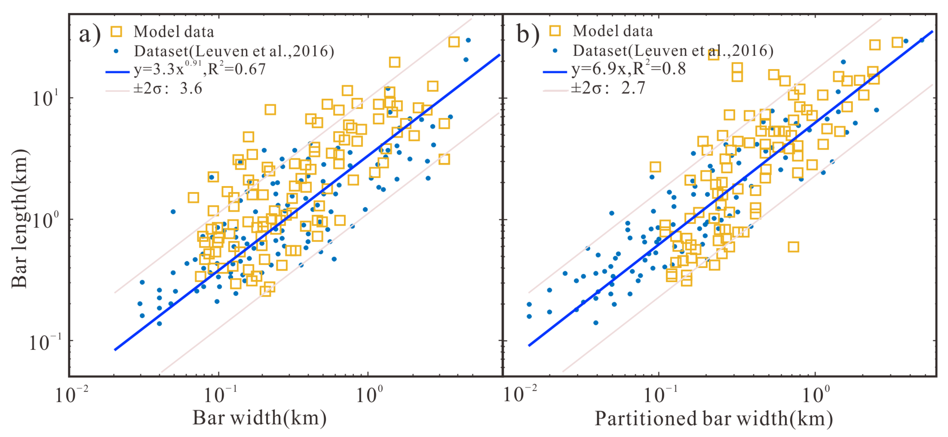
The simulated estuary shape is characterized by an ideal funnel shape [40]. The model domain is 36 km × 100 km, comprising part of the fluvial zone, estuary area, and ocean area (Figure S1). The model comprises equal grids with a resolution of 200 m × 160 m, and the grid aspect ratios align consistent with the geometry of the funnel-shaped estuary. Following grid refinement, it facilitates the observation of more morphological details, such as smaller tidal channels and smaller-sized bar features [41]. The grid size is kept constant to improve the simulation convergence. The straight river is 15 km in length and 1.92 km in width, flowing into the inner estuary area (Figure 1). The length of the estuary area is set to be 45 km. The width of the estuary area increases from 2 km at the fluvial inlet to 30 km at the mouth of the estuary (Figure 1). The ocean area has a length of 40 km and width of 36 km. The bed level decreases linearly from the upstream fluvial boundary to the mouth of the estuary, and the overall slope of the model is set to 0.017 (Figure S2). The water depths are set to 8 m at the fluvial boundary and 28 m at the mouth of the estuary. This forms the estuary at the end of the rising sea-level cycle, and the sea level remains constant during the model runs [3]. The schematic of the model settings is shown in Figure 1.

Discharge boundary and open sea boundary are the open boundary conditions used. The average current, tidal frequency, and tidal range height of modern estuaries can provide reference for the model parameters [27,28,42,43]. We set the total fluvial discharge to a constant value of 3000 m³s⁻¹ to keep a sufficient and stable source supply for the estuary (

Table 1. Initial parameter type, initial value, and range of the default model.

Parameter	Symbol	Unit	Value	Range
Initial water depth	-	m	28	-
Discharge	-	m3s−1	3000	1500–4500
Tidal amplitude	-	m	6.7	3.4–7.2
Time step	dt	min	0.5	0–999
Threshold sediment thickness	-	m	0.05	0.005–10
Threshold depth	-	m	0.1	0–10
Min water depth for bed level change	SedThr	m	0.1	0.1–10
Morphological scale factor	H	-	100	1–400
Number of under layers	MxNULyr	-	400	-
Thickness of each under layer	ThUnLyr	m	0.1	-
Thickness of the transport layer	ThTrLyr	m	0.2	-
Erosion of adjacent dry cells	-	-	0.5	0–1

). The tidal boundary condition is the semidiurnal tide with a tidal amplitude of 6.7 m, providing continuous seaward transport power for estuary sediments (Table 1). For ensuring stability and accuracy, a time step of 0.5 min is used. The simulation time is set to 1 yr with a morphological scale factor of 100, which is comparable to a century of sedimentary evolution [41]. Although the large-scale time span of the simulation, the effects of the sea level change and organisms are ignored for generalization and simplicity. The stratigraphic record of the estuary sedimentation sequence is updated in each time step, including the bed level and stratigraphic sediment thickness (Table 1) [44,45]. The sediment subsurface is shown according to a multilayer concept [44,46]; hence, the virtual sedimentary successions of the estuary are set to 400 layers, each with a thickness of 0.1 m [41]. The underlayer fixed substrate tracks the sediment composition over time in the vertical direction. If the remaining sediment thickness is less than the sediment thickness threshold of 0.05 m and erosive conditions are expected. Above the underlayer, a transport layer of 0.2 m is used to exchange the sediment with the fluid layer (Table 1). To stabilize the complex hydrodynamic calculation, a factor for the erosion of adjacent dry cells is specified that determines the proportion of erosion evenly distributed to the adjacent cells. This factor is 0.5 in our simulation, meaning that half of the erosion that occurs in wet cells is distributed to adjacent dry cells [41].

The majority of the sediment supplied to estuaries consist of sand, with mud components and salt marshes [7]. Hence, noncohesive sand sediment and cohesive mud sediment are the sediment components used in the model [47]. For sediment supply, the flow carries sand and mud that supply the estuary area at a fixed concentration, meaning that sediment delivery to the model depends on hydrodynamic conditions. The total sediment supply is set to 7 kgm⁻³ in the simulation. Two types of noncohesive sand sediment components and three types of cohesive mud sediment components are used.

Table 2. Sediment fraction types and parameter settings for each sediment component in the models.

Sediment Component	Type	Median Sediment Diameter (μm)	Setting Velocity (mms−1)	Critical Bed Shear Stress for Sedimentation (Nm−2)	Critical Bed Shear Stress for Erosion (Nm−2)
Sand1 (S1)	NonCohesive	125	-	-	-
Sand2 (S2)	NonCohesive	80	-	-	-
Mud1 (M1)	Cohesive	-	0.86	1000	0.3
Mud2 (M2)	Cohesive	-	0.25	1000	0.5
Mud3 (M3)	Cohesive	-	0.16	1000	0.6

lists each sediment component property. Cohesive sediment components are defined in terms of setting velocity and critical bed shear stress rather than grain size [48], wherein the default setting velocity is 0.25 mms⁻¹, critical shear stress for erosion is 0.5 Nm⁻², and critical shear stress for sedimentation is 1000 Nm⁻². If the bed shear stress for sedimentation of the cohesive sediment fractions is larger than the critical value, no sedimentation occurs; otherwise, mixed sediment fluxes are calculated following the Partheniades–Krone equations.

A specific model parameter space is designed for investigating the effects of sediment composition and transport on estuary evolution (

Table 3. Parameter list of all model scenarios.

Model Scenario	Type	Case ID	Fluvial Mud (kgm−3)	Sediment Class	Tidal Amplitude (m)	Discharge (m3s−1)	Note
Base model	default	01	1.75	S1 S2 M2	6.7	3000	Fluvial mud input
Mud supply	mud concentration	02	3.5	S1 S2 M2	6.7	3000	Higher fluvial mud
		03	0	S1 S2	6.7	3000	No mud, only sand
	mud transport properties	04	1.75	S1 S2 M1	6.7	3000	Higher mud cohesive
		05	1.75	S1 S2 M3	6.7	3000	Lower mud cohesive
Hydrodynamic condition	tidal amplitude	06	1.75	S1 S2 M2	3.4	3000	Lower tide
		07	1.75	S1 S2 M2	7.2	3000	Higher tide
	fluvial discharge	08	1.75	S1 S2 M2	6.7	1500	Lower discharge
		09	1.75	S1 S2 M2	6.7	4500	Higher discharge

). The model is run in nine estuary scenarios under the same initial conditions. The model scenarios are analyzed by studying the effect of mud concentration, mud transport properties, tidal amplitude, and fluvial discharge on the sedimentary characteristics. Fluvial mud supply concentration at the upstream boundary is varied to assess the effect of mud concentration on estuary morphology. The effect of mud transport characteristics is further discussed by comparing scenarios with mud inputs with different setting velocities and erosion shear stress. Common factor analysis is used to further study the role of fluvial discharge and tidal amplitude on sedimentary distribution and to clarify the main factors that control the mud distribution characteristics in estuaries. These simulation results are quantitatively analyzed and compared to each other. Finally, the simulation results are compared with data from real estuaries.

The sedimentary characteristics are presented in the form of a map, which assesses the sedimentary distribution and tidal bar morphology or cross-sectional view to enable the study of channel depth variation and sediment thickness evolution. From the three-dimensional sedimentary data, cumulative sedimentation and erosion are further calculated. The sedimentary components are tracked along with the vertical and horizontal directions, and each x and y coordinate point in the model space is recorded to represent the change in the corresponding bar elevation, i.e., decreasing elevation reflects the erosion process and increasing elevation reflects the deposition process [14].

3. Results

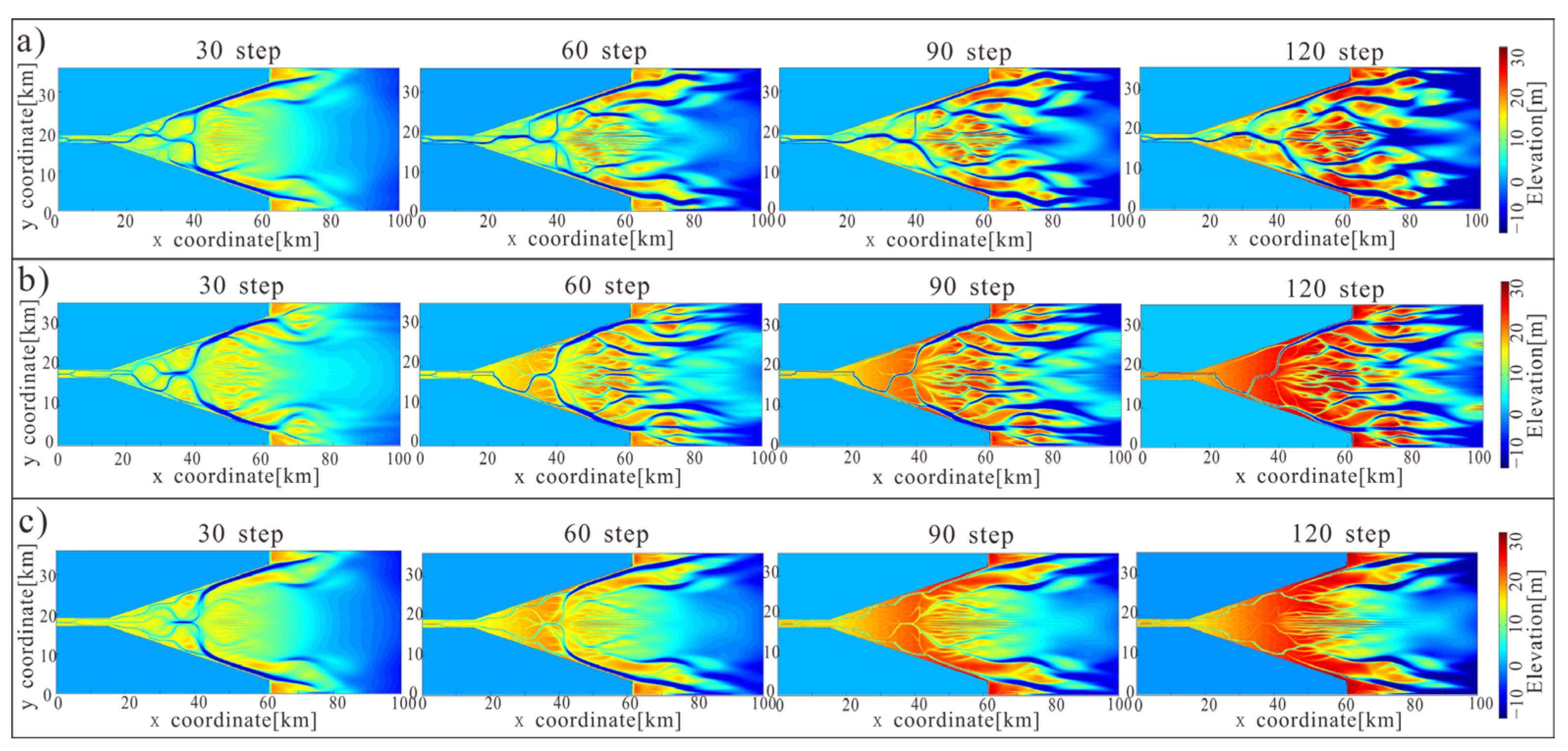
3.1. Effect of Mud Concentration on the Sedimentary Characteristics

For analyzing the effect of mud concentration on sediment characteristics, three sets of comparative scenarios are set, namely, no mud supply (zero mud concentration), lower mud concentration, and higher mud concentration (Table 3). In the simulation, mud supply concentration is changed by adjusting the sand–mud ratio and the total sediment supply is set constant. The sand–mud ratio of the smaller mud concentration model is 3:1, and the sand–mud ratio of the larger mud concentration model is 1:1 (Table 3).

The number of bar and tidal channel morphologies changes considerably with changing the supply of mud concentration (Figure 2). For the case with no mud supply (Case 03), the tidal channel in estuaries has a high degree of cutting and a large number of tidal bars (Figure 2a). Compared to Case 01, when the mud concentration is 1.75 kgm⁻³, the degree of development of the tidal bar in the inner estuary is not high, but tidal bar thickness increases (Figure 2b). Tidal channels develop in the middle and outer estuaries, which become more braided owing to unhindered bank erosion. For the mud concentration of 3.5 kgm⁻³ (Case 02), sediment diffusion becomes slight, and the tidal bar has a high degree of sedimentation in the inner estuary (Figure 2c). Compared with Cases 01 and 03, the tidal channels for higher mud concentration mainly develop in the middle of the river, which are straighter and less migrated. Figure 2 shows that the number of tidal bars decreases with increasing mud concentration and channel migration decreases greatly. Hence, it is concluded that the presence of mud components prevents sediment transport and increases erosion resistance, affording more stable tidal bars and banks.

In Figure 3, erosion is obvious in the channel without mud supply at the beginning of the simulation, with a mean channel depth of 3.23 m (Figure 3a). The number of active channels and the mean channel depth decrease when the mud concentrations are 1.75 and 3.5 kgm⁻³, with mean channel depths of 2.58 m and 1.59 m, respectively (Figure 3a). At the end of the simulation, the sand-based estuary forms a deeper channel incision, and the mean depth of the channel is 4.21 m (Figure 3b). In the model with mud concentration of 3.5 kgm⁻³, the mean channel depth is 2.02 m, and the erosion rate is 28% lower than that of the no mud supply model. In addition, the mean channel depth is 3.61 m in the inner estuary, and the mean channel depths of the middle and outer estuaries are 3.80 m and 4.04 m, respectively. The mean channel depth tends to increase as the distance increases from the supply source (Figure 3c). This is because the fluvial mud input enhances the mud deposition at the top of the inner estuary and causes the silting of mud components in the channel. The above simulation results indicate that mud components tend to deposit in the channel and the inner estuary with increasing mud concentration. These mud-dominated sediments are resistant to erosion, thus slowing down the erosion rate and reducing the tidal bar mobility.

Mud concentration has a significant effect on the thickness and distribution of mud deposits in the estuary. When there is no mud supply, mud deposits derived from the initial stratigraphy are stirred up by the fluvial flows and tides and 90% of the mud deposits are thinner than 0.47 m. When the mud concentration is 1.75 kgm⁻³, 50% of the mud-deposit thickness is less than 0.36 m and 90% of the mud-deposit thickness is less than 1.80 m in estuary sedimentation. For the mud concentration of 3.5 kgm⁻³, 50% of the mud-deposit thickness is less than 0.36 m and 90% of the mud-deposit thickness is less than 1.92 m. Mud-dominated sediment aggradation occurs more rapidly with increasing mud concentration, yielding thicker mud deposits and higher bed levels. The simulation results herein indicate that the higher the mud concentration, the greater the mud-deposit thickness, and the stronger the self-confinement of the estuary. This self-confinement leads to a smaller surface area and narrower estuaries, eventually affecting the sedimentary characteristics of estuaries. In addition, there is an inevitable relationship between estuary morphology and sediment supply [49].

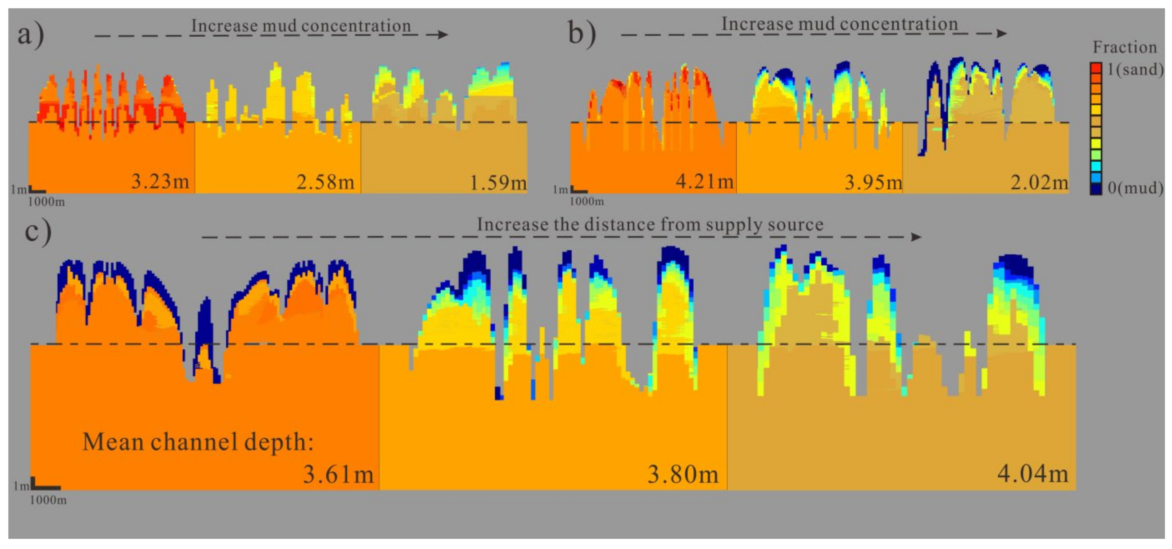
3.2. Effects of Mud Transport Properties on the Tidal Bar Characteristics

The mud transport properties cause complicated processes acting on sediment erosion and deposition under physicochemical forces [50]. This section focuses on the effects of mud transport properties, namely, settling velocity and erosion shear stress on mud deposition (Figures S3 and S4). Table 2 and Table 3 list the parameter settings for each sediment component and the type of mud component for each scenario, respectively.

The simulation results show that the morphological characteristics are less affected by the change in mud transport properties at the early stage of simulation. However, significant changes occur in tidal channel development as the simulation continues. For higher and medium settling velocities (Cases 03 and 04; Case 01), the sediment deposition rate is faster in the inner estuary with an average sediment thickness of more than 20 m (Figure 4a,b). At the beginning of the simulation, multiple channels are developed in the inner estuary, the sediment is deposited along both sides of the bed and channel in the inner estuary, and the channels are developed on both sides simultaneously. For higher settling velocity, at the end of the simulation, these also happen (Figure 4a). For medium settling velocity, at the end of the simulation, the sediment accumulates in the inner estuary, which makes part of the channel fill with sediment and develop a single channel (Figure 4b). The estuary with a lower settling velocity shares many similarities in geomorphic morphology with the no mud model. For the lower settling velocity (Case 05), relatively large channel mobility and mean channel depth are observed (Figure 4c). From the perspective of the inner and outer estuaries, the channel is better developed in the inner estuary and the tidal channel is wide and deep in the outer estuary (Figure 4c). Comparing Cases 01, 04, and 05, as the settling velocity decreases, the degree of sediment diffusion increases and the thickness of sediment decreases.

The length, width, and thickness distribution of the bar are further calculated based on the simulation results to quantitatively influence the mud sediment properties on the scale of the tidal bar [51]. The thickness of the tidal bar increases with increasing distance from the estuary mouth. In the higher settling velocity simulation scenario (Case 04), average tidal bar thicknesses in the inner and outer estuaries of 8.2 and up to 28 m are measured (Figure 5a). For lower settling velocity (Case 05), there is an increased average tidal bar thickness from 4 to 19.8 m from the inner estuary to the outer estuary (Figure 5a). The thickness of tidal bars gradually becomes thinner near the ocean area. The tidal bar width is microscopically affected by location and the setting velocity, and the distribution is concentrated between 1 and 4 km (Figure 5b). To be more specific, the tidal bar shape varies with the mud transport properties. In a sediment supply system with a lower setting velocity (Case 05), the RLW values of the tidal bar vary from 1 to 5 (Figure 5c). The higher setting velocity has a great influence on the RLW of the tidal bar, and the ratio is mainly concentrated from 4 to 15 (Case 04; Figure 5c). In addition, the tidal bar increasingly tends to become a long strip and the RLW is higher with increasing distance from the estuary mouth (Figure 5c). This is because the bar has a tendency of avulsion under a strong hydrodynamic disturbance while being protected by the strong cohesion of mud fractions, yielding a strip-shaped bar morphology. More specifically, the tidal bar shape varies with the mud transport properties. In a sediment supply system with a lower setting velocity (Case 05), the RLW value of the tidal bar mainly vary between 1 and 5 (Figure 5c). The higher setting velocity has great influence on the RLW of tidal bar, and the ratio is mainly concentrated between 4 and 15 (Case 04; Figure 5c). Furthermore, the tidal bar increasingly tends to become long strip shape and the RLW is higher as the distance from the estuary mouth increases (Figure 5c). This is because the bar has a tendency of avulsion under the strong hydrodynamic disturbance and, at the same time, it is protected by the strong cohesion of mud fractions. Hence, settling velocity is one of the key factors affecting the development of bar morphology.

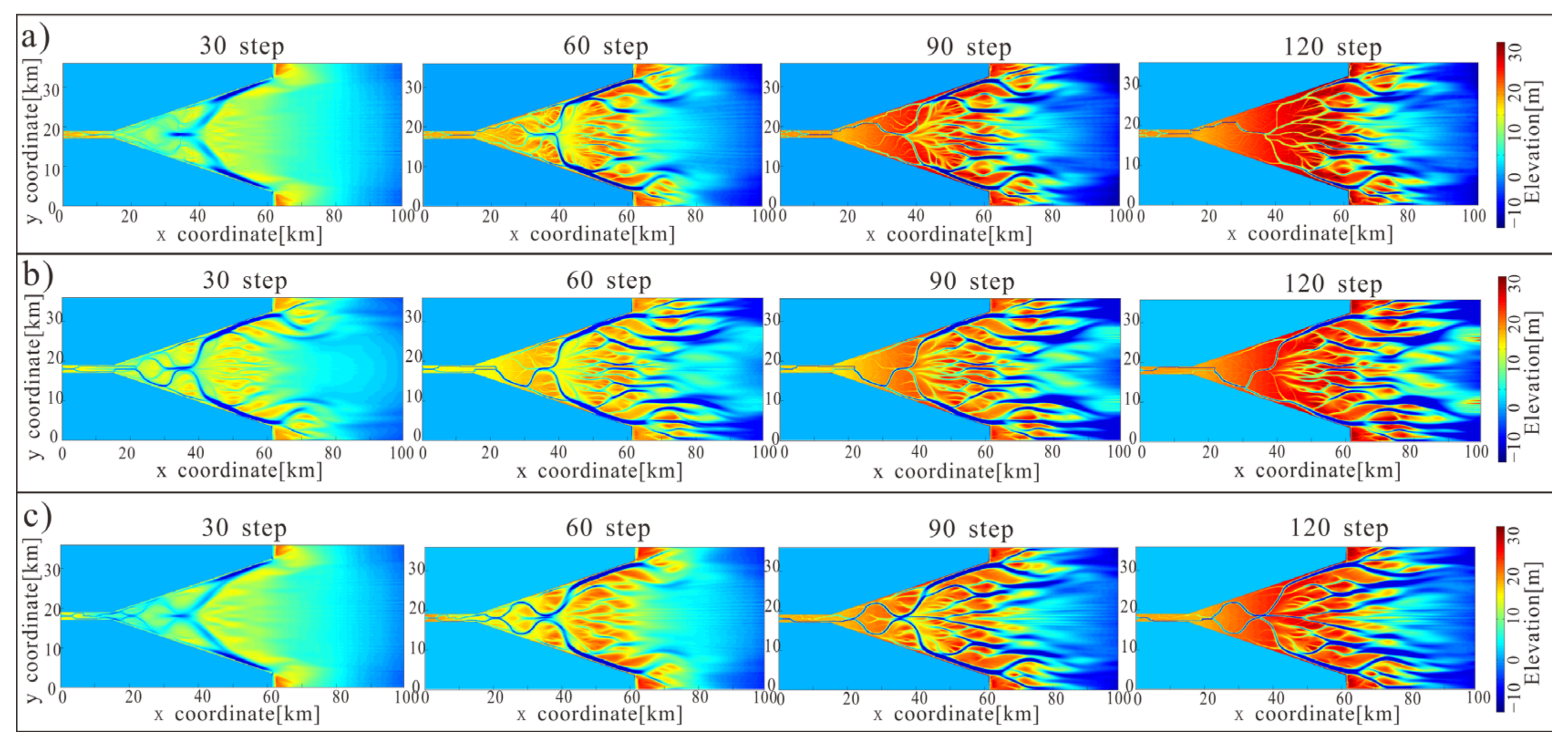
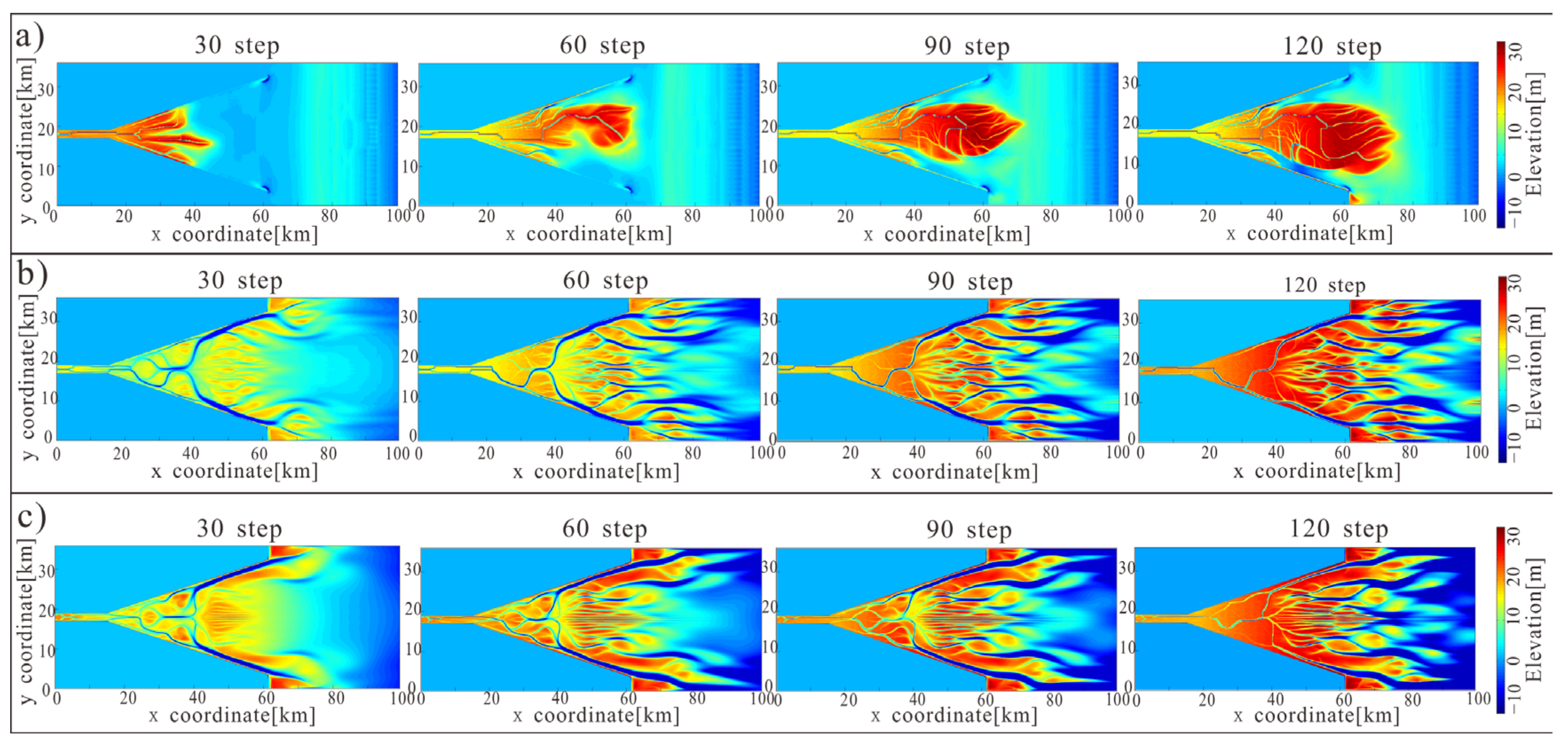
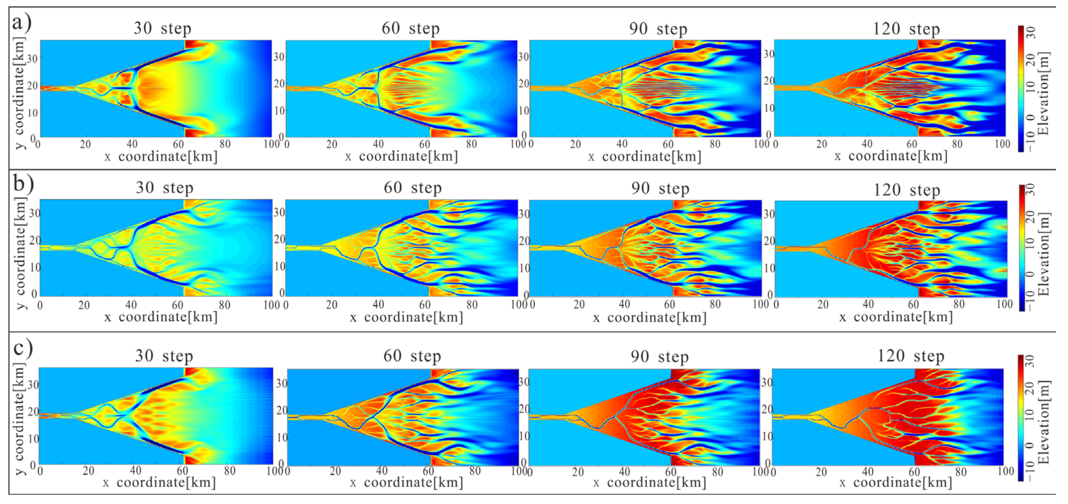
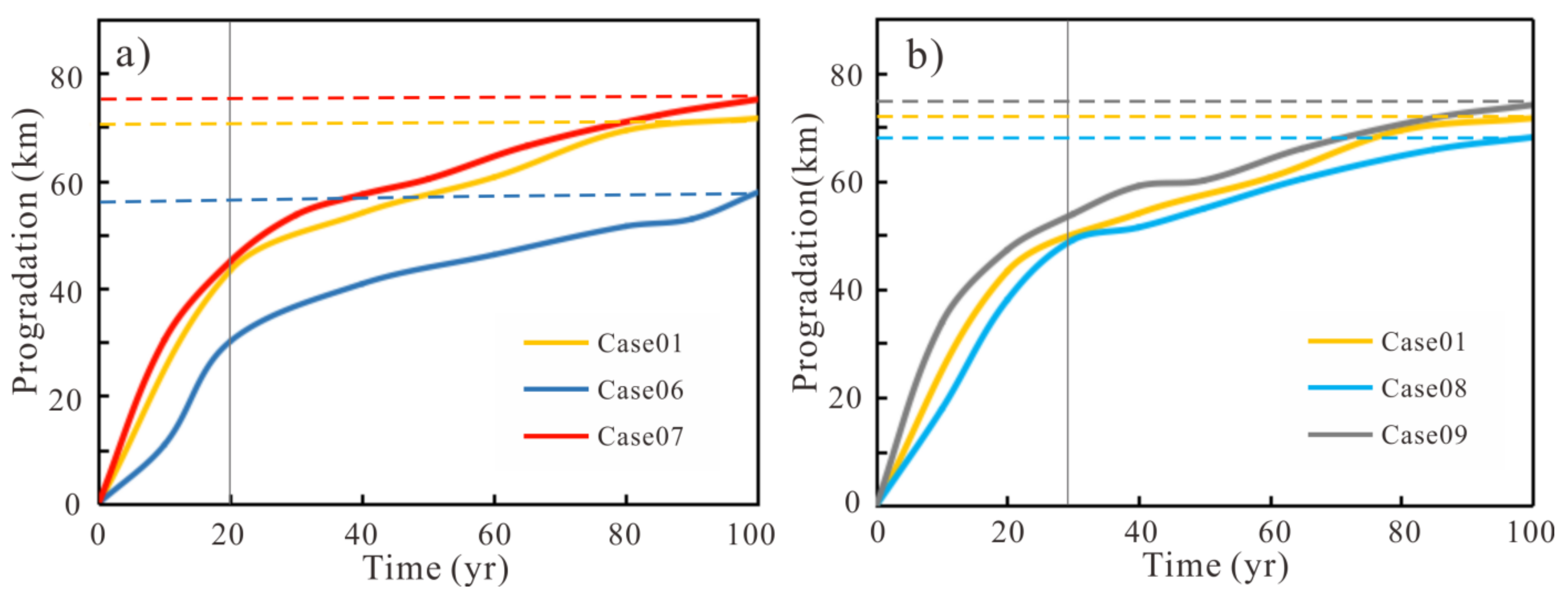
3.3. Effects of Hydrodynamic Conditions on the Sedimentary Distribution in Estuaries

In estuaries, tides are the most important driving force for sediment transport, and fluvial discharge plays an important role in sediment source supply. The interaction of tidal amplitude and fluvial discharge in estuaries has led to a continuously evolving morphology with river channels and bars. In this section, the effects of hydrodynamic conditions on sedimentary distribution are analyzed by changing tidal amplitudes and fluvial discharges. Table 3 lists the specific parameter settings.

It is concluded that the development degree of the tidal bar changes obviously with tidal amplitude (Figure 6). With a lower tidal amplitude of 3.4 m (Case 06), the inner estuary is covered with mud deposition and shows slight progradation (Figure 6a). Although the sediment thickness is the highest among the case of tidal amplitudes (mean 25 m), the tidal bar has not developed very well, only with a mean thickness of 2.1 m. This is because the fluvial sand-carrying and sand-flushing plays a dominant role in estuaries, the tidal action is extremely weak, and hence, there is almost no sediment being reprocessed. For the estuary with a medium tidal amplitude of 6.8 m (Case 01) and higher tidal amplitude of 7.2 m (Case 07), the inner estuary develops multiple deeper channels. In the outer estuary, the tidal bar is well developed with a more complex shape owing to erosion and redeposition (Figure 6b,c). The increased tidal amplitude makes the sediment deposit farther seaward, yielding a smaller mean sediment thickness in the entire estuary. In summary, the greater the tidal amplitude, the greater the degree of the seaward migration of the tidal bar and the deeper is the erosion of tidal channels.

The simulation results show that fluvial discharge considerably affects the development rate and sediment thickness of tidal bars. For lower fluvial discharge (Case 08), the tidal bar exhibits an elliptical shape in the inner estuary of ~4.5 m thickness (Figure 7a). For higher fluvial discharge (Case 09), the inner estuary bars appear to be an elongated shape, with a faster development rate (Figure 7c). In addition, the tidal bars gradually develop to a complex bar. The higher the fluvial discharge, the higher the deposition rate. In the later stage of the simulation, the sediments are concentrated in the middle and outer estuaries, where the sediment thickness is the largest. Based on the simulation results, this implies that river-dominated estuaries form larger and thicker deposits, which more easily cause the transition from filled estuaries to deltas [13,52].

The evolution of sediment progradation in Figure 8 shows that the range of sediment progradation in estuaries is concentrated at 70 km under the three fluvial discharge conditions, indicating a slight effect of fluvial discharge on sediment transport distance. The increase in tidal amplitude brings an obvious prograde seaward. The progradation area in the lower tidal amplitude accounts for 53% of the estuary (Figure 8a), and the range of the progradation is ~58 km. The progradation area can reach the entire estuary in the higher tidal amplitude (Figure 8b). This indicates that tidal energy is the major factor that determines the range of sediment progradation in estuaries [15]. In addition, the higher fluvial discharge with higher tidal amplitude keeps the sediment in a suspended state, affording a more dynamic system. When the discharge is high and the tidal amplitude is low, the estuary fills and eventually evolves into a delta. This finding demonstrates that in the absence of a sea-level rise and fall, hydrodynamic conditions are enough to alter sediment retrogradation and progradation behavior [2,53].

4. Discussion

4.1. Comparison with Modern Sedimentation

The development of tidal bars and the sedimentary distribution characteristics in estuaries change with the changes of various factors. Based on sedimentary dynamic simulations, we quantified the effects of mud concentration, mud transport properties, tidal amplitude, and fluvial discharge on the sedimentary characteristics of the estuary. The numerical simulation results indicate that tidal amplitude plays a major role in tidal bar morphology. The greater the tidal amplitude, the higher the degree of development of tidal bars in estuaries, consistent with Schramkowski et al. [19]. Mud concentration and fluvial discharge also have a significant effect on estuary sediment thickness. With a higher mud concentration, relatively higher fluvial discharge, and lower tidal amplitude, the estuary sediment thickness becomes larger and the deposition area becomes wider, which is in good agreement with the simulation results of Hibma et al. [54].

The sediment in the models is similar to modern estuaries in terms of their distribution characteristics and behavior. There is a relatively large proportion of erosion sediments on both sides of the channel in the simulation results (Figure 4), forming mudflat deposition in agreement with the characteristics of modern estuary datasets [55]. There are fewer mud deposits in the center of the outer estuary compared to mudflats along the flank of the basin, and a similar pattern has been observed in the Western Scheldt [16,50]. The Scheldt estuary consists mainly of sand with a small amount of mud deposition [47]. The estuary has a freshwater discharge of 120 m³s⁻¹, and fluvial mud supply is 100 × 10⁶ kgyr⁻¹ [47]. Likewise, the Scheldt estuary supplied mud deposition from a single channel as in the simulated model.

Figure 9 demonstrates the cumulative probability distribution of mud-deposit thickness covering the top of the modeled estuary and Scheldt estuary. Average mud-deposit thicknesses of the modeled and Scheldt estuaries are 1.0 and 1.2 m, respectively (Figure 9). This is because the mud input in the Scheldt estuary is ~15% higher [13]. Here, the mud-deposit thickness of the Scheldt estuary increases from 1.3 m near the head to 2.7 m near the mouth [47]. About 60% of the mud-deposit thickness obtained from the models is less than 0.5 m, and 90% of the mud-deposit thickness is concentrated from 0.05 to 3.0 m (Figure 9), in general accordance with the Scheldt estuary of sediment distribution. From the above statistical characteristics of sediment thickness, the simulated estuary is in good agreement with modern sedimentation.

Comparing the dimensions of individual tidal bars from the datasets collected by Leuven et al. [55] with the tidal bars of the simulation results, it is found that the aspect ratios of the tidal bars are in the range of 3–10. The lengths of tidal bars in our simulations are concentrated at ~10 km, and the widths are distributed at 1.5 km and partitioned bar widths are distributed at 0.8 km (Figure 10), with a similar scatter to the datasets. Most of the simulated scatter points are distributed within the range of higher or lower confidence limit trends, and the tidal bars are close to the modern estuary bar size. Meanwhile, the bar morphology in the estuary models is consistent with the natural bar. A natural estuary is developed from the seaward direction with a sidebar, distributary bar, compound bar, U-shaped bar, and linear bar. The simulation herein shows that the linear bars are concentrated in the outer estuary, especially in the case with a tidal amplitude of 7.2 m (Figure 6). The U-shaped bars appear in the middle of the outer estuary, and the compound bars are stored in the inner estuary at the later stage of the simulation. The distributary bars are the most obvious in the case with a fluvial discharge of 1500 m³s⁻¹ (Figure 7). From the comparative analysis of statistical data, the sedimentary characteristics of estuaries obtained using the sedimentary dynamic numerical simulation method are in good agreement with modern sedimentation characteristics.

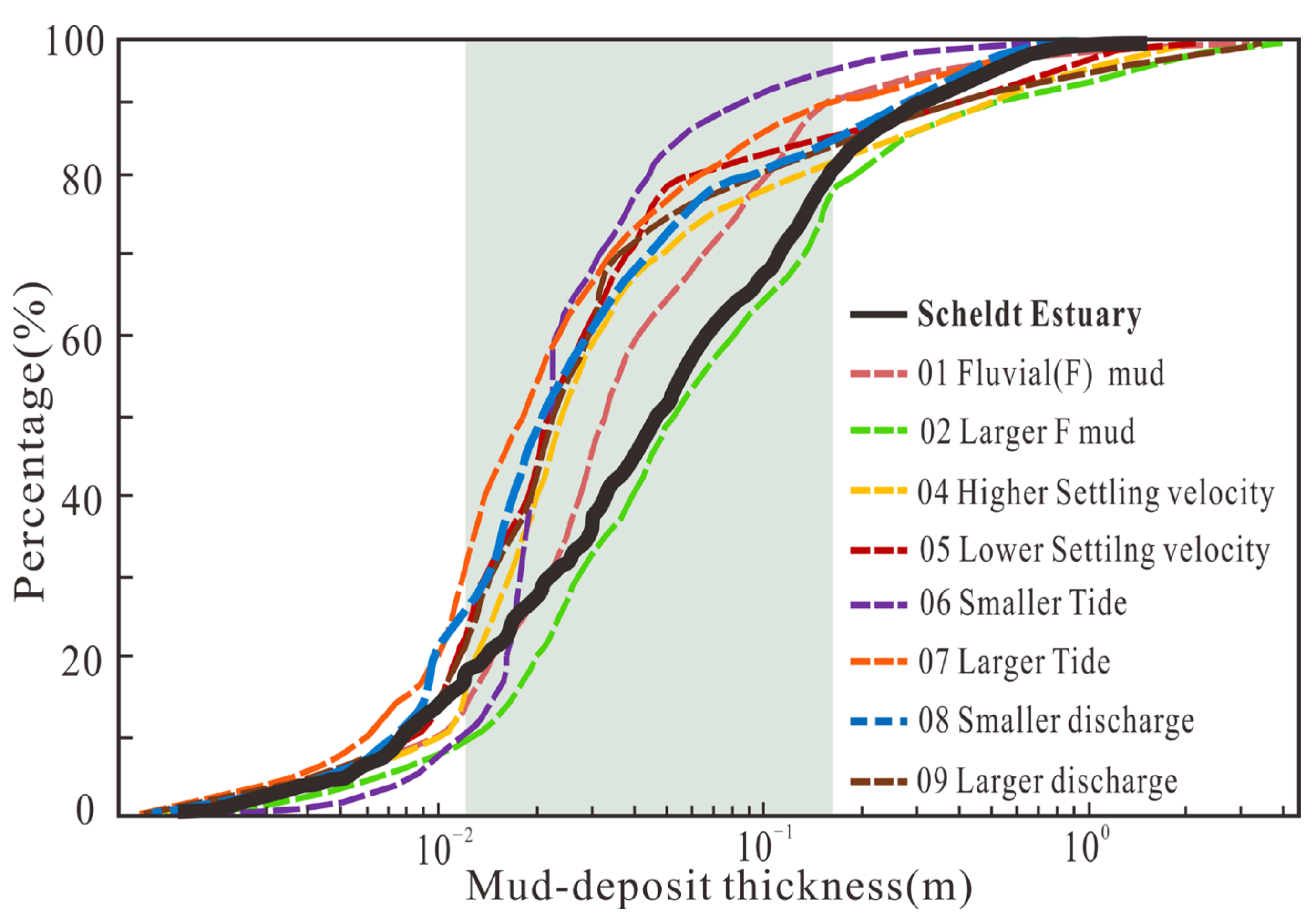
4.2. Distribution of the Mud Deposits

Mud deposits are mainly stored in the estuary in two forms. Most of the mud is deposited at the top of the estuary in the form of mudflats, and a small amount is deposited in the middle of the bar as mud interlayers. The mud interlayer is formed in connection with the sedimentary environment, and the banded mudstone wall easily develops [56]. The estuary model reproduces the three-dimensional internal structure of the mud interlayer, enabling us to further study the quantified distribution of interlayers in modern estuaries. Based on the statistical data, the thickness of the mud interlayer is concentrated in 0.4–0.6 m, and a small part of the mud interlayer can reach 1.5 m thickness (

Table 4. Descriptive statistics of the sediment progradation and the mud interlayers in the estuary model.

Case ID	Average Sediment Progradation (km)	Length of Mud Interlayer (km)	Thickness of Mud Interlayer (m)	Distribution Frequency (Pieces)
01	67.3	4.93	0.47	1.23
02	60.8	5.41	0.52	0.98
03	70.1	-	-	-
04	58.8	5.59	0.50	0.92
05	62.0	7.03	0.32	1.20
06	57.5	2.47	0.28	0.48
07	75.4	7.19	0.39	0.57
08	65.3	3.89	0.41	0.68
09	69.6	5.43	0.72	1.05

). The length of mud interlayers varies considerably, with some of them concentrated in 2–4 km and others concentrated in 8–10 km, with the maximum length of the mud interlayer reaching 16 km (Table 4).

The increased mud concentration has a positive feedback effect on the length and thickness of the mud interlayer (Table 4) [56]. Conversely, the alteration of mud concentration is opposite to the sediment progradation, in which the higher mud concentration cases restrict seaward progradation (Table 4). The average mud interlayer thickness and length are similar in most cases and no significant trend for changing mud properties or mud supply sources is observed. The effect of hydrodynamic conditions is intense for the internal structure of the mud interlayer [56]. The thickness of the interlayer increases with increasing fluvial discharge, but the length of the interlayer varies poorly with fluvial discharge. Under the smallest discharge, the interlayer length is the smallest (Table 4). With increasing tidal intensity, the thickness of the interlayer decreases, while the length of the interlayer increases and changes (Table 4). The above observations suggest that the tide is the main controlling factor and fluvial current is a secondary controlling factor for the length of the interlayer. For the thickness of the interlayer, the fluvial currents exerted the primary control and tides had a secondary effect. The quantitative statistics of the thickness and distribution of mud interlayer are of great significance for the classification and understanding of the internal architecture of estuaries [56].

5. Conclusions

A process-based numerical simulation method is proposed to investigate the effect of mud supply and hydrodynamic conditions on the sedimentary development and distribution in estuaries. Our model demonstrates the effect of mud supply, sediment transport, and hydrodynamic conditions on the long-term evolution of estuaries. The statistical data obtained using this the model provide a quantitative analysis of the process–product relationship in estuaries. A series of morphological maps and cross-sectional view results show that the estuary develops into dynamic channels and sandbars flanked by mudflats, and the thickness is in the range of 1–2 m. About 60% of the thickness of mud deposits is between 0.21 m and 0.36 m, and 90% of the mud deposits are more than 0.69 m thick. Meanwhile, a small amount of mud is deposited in the middle of the bar as mud interlayers. The thickness of the mud interlayer is concentrated from 0.4 to 0.6 m; however, the length varies considerably, up to 16 km. The study concludes that mud supply strengthens self-confinement, and a higher mud concentration yields stable tidal bars and banks as well as reduced channel migration. Conversely, the estuary without mud supply is less resistant to erosion and more highly incised; thus, there are more tidal bars. Mud transport properties considerably affect the tidal bar morphology. The estuary tidal bar with a higher settling velocity has a high degree of development and a larger length-to-width ratio, mainly forming a long strip tidal bar. The study of hydrological conditions focuses on rivers and tides, and fluvial discharge and tidal amplitude form negative feedback on the dynamic balance between deposition and erosion. When the fluvial discharge is low and the tidal amplitude is high, mud deposits are suspended in the estuary so that less mud settles. Meanwhile, with lower fluvial discharge and higher tidal amplitude, the estuary fills up and eventually becomes a tidal delta. The sediments in the models are in good agreement with sedimentation in modern estuaries in terms of their distribution characteristics and behavior. It is hoped that the sedimentary dynamic numerical simulation method used herein can help predict variations in stratigraphic structures and provide guidance for the further exploration and development of estuary sedimentary reservoirs.

References

1. Galloway, W.E. Process Framework for Describing the Morphologic and Stratigraphic Evolution of Deltaic Depositional Systems; Houston Geological Society: Houston, TX, USA, 1975; pp. 87–98. [Google Scholar]
2. Dalrymple, R.W.; Zaitlin, B.A.; Boyd, R. Estuarine Facies Models: Conceptual Basis and Stratigraphic Implications. J. Sediment. Res. 1992, 62, 1130–1146. [Google Scholar] [CrossRef]
3. Dalrymple, R.W.; Choi, K. Morphologic and facies trends through the fluvial–marine transition in tide-dominated depositional systems: A schematic framework for environmental and sequence-stratigraphic interpretation. Earth-Sci. Rev. 2007, 81, 135–174. [Google Scholar] [CrossRef]
4. Gugliotta, M.; Saito, Y.; Van Lap, N.; Thi Kim Oanh, T.; Nakashima, R.; Tamura, T.; Uehara, K.; Katsuki, K.; Yamamoto, S. Process regime, salinity, morphological, and sedimentary trends along the fluvial to marine transition zone of the mixed-energy Mekong River delta, Vietnam. Cont. Shelf Res. 2017, 147, 7–26. [Google Scholar] [CrossRef]
5. Van der Wegen, M.; Wang, Z.B.; Savenije, H.H.G.; Roelvink, J.A. Long-term morphodynamic evolution and energy dissipation in a coastal plain, tidal embayment. J. Geophys. Res-Earth Surf. 2008, 113, F03001. [Google Scholar] [CrossRef] [Green Version]
6. Gugliotta, M.; Saito, Y.; Nguyen, V.L.; Ta, T.K.O.; Tamura, T. Sediment distribution and depositional processes along the fluvial to marine transition zone of the Mekong River delta, Vietnam. Sedimentology 2019, 66, 146–164. [Google Scholar] [CrossRef]
7. Dalman, R.; Weltje, G.J.; Karamitopoulos, P. High-resolution sequence stratigraphy of fluvio-deltaic systems: Prospects of system-wide chronostratigraphic correlation. Earth Planet. Sci. Lett. 2015, 412, 10–17. [Google Scholar] [CrossRef]
8. Van Ledden, M.V.; Kesteren, W.; Winterwerp, J.C. A conceptual framework for the erosion behaviour of sand–mud mixtures. Cont. Shelf Res. 2004, 24, 1–11. [Google Scholar] [CrossRef]
9. Le Hir, P.; Cayocca, F.; Waeles, B. Dynamics of sand and mud mixtures: A multiprocess-based modelling strategy. Cont. Shelf Res. 2011, 31, S135–S149. [Google Scholar] [CrossRef] [Green Version]
10. Schuurman, F.; Shimizu, Y.; Iwasaki, T.; Kleinhans, M.G. Dynamic meandering in response to upstream perturbations and floodplain formation. Geomorphology 2016, 253, 94–109. [Google Scholar] [CrossRef]
11. Dalrymple, R.W.; Baker, E.K.; Harris, P.T.; Hughes, M.G. Sedimentology and Stratigraphy of a Tide-Dominated, Foreland-Basin Delta (Fly River, Papua New Guinea). In Tropical Deltas of Southeast Asia; SEPM (Society for Sedimentary Geology): Tulsa, OK, USA, 2003; pp. 143–173. [Google Scholar]
12. Fenies, H.; Tastet, J.P. Facies and architecture of an estuarine tidal bar (the Trompeloup bar, Gironde Estuary, SW France). Mar. Geol. 1998, 150, 149–169. [Google Scholar] [CrossRef]
13. Van de Lageweg, W.I.; Braat, L.; Parsons, D.R.; Kleinhans, M.G. Controls on mud distribution and architecture along the fluvial-to-marine transition. Geology 2018, 46, 971–974. [Google Scholar] [CrossRef] [Green Version]
14. Van de Lageweg, W.I.; Feldman, H. Process-based modelling of morphodynamics and bar architecture in confined basins with fluvial and tidal currents. Mar. Geol. 2018, 398, 35–47. [Google Scholar] [CrossRef]
15. Winterwerp, J.C. Fine sediment transport by tidal asymmetry in the high-concentrated Ems River: Indications for a regime shift in response to channel deepening. Ocean Dyn. 2011, 61, 203–215. [Google Scholar] [CrossRef] [Green Version]
16. Verlaan, P. Marine vs Fluvial Bottom Mud in the Scheldt Estuary. Estuar. Coast. Shelf Sci. 2000, 50, 627–638. [Google Scholar] [CrossRef]
17. Cleveringa, J.; Dam, G. Slib in de Sedimentbalans van de Westerschelde; Eindrapport G-3, 1630/U12376/C/GD; Vlaams Nederlandse Scheldecommissie: Bergen op Zoom, The Netherlands, 2013. [Google Scholar]
18. Kleinhans, M.G. Sorting out river channel patterns. Prog. Phys. Geogr 2010, 34, 287–326. [Google Scholar] [CrossRef]
19. Schramkowski, G.P.; Schuttelaars, H.M.; de Swart, H.E. The Effect of Geometry and Bottom Friction on Local Bed Forms in a Tidal Embayment. Cont. Shelf Res. 2002, 22, 182–1833. [Google Scholar] [CrossRef]
20. Toffolon, M.; Crosato, A. Developing Macroscale Indicators for Estuarine Morphology: The Case of the Scheldt Estuary. J. Coast. Res. 2007, 231, 195–212. [Google Scholar] [CrossRef]
21. Tessier, B. Stratigraphy of tide-dominated estuaries. In Principles of Tidal Sedimentology; Davis, R.A., Jr., Dalrymple, R.W., Eds.; Springer: Dordrecht, The Netherlands, 2012; pp. 109–128. [Google Scholar]
22. Sprovieri, M.; Bonanno, A.; Mazzola, S.; Patti, B. Cyclostratigraphy: A methodological approach. Riv. Ital. Paleontol. Stratigr. 2002, 108, 179–182. [Google Scholar] [CrossRef]
23. Die Moran, A.D.; Abderrezzak, K.E.K.; Mosselman, E.; Habersack, H.; Lebert, F.; Aelbrecht, D.; Laperrousaz, E. Physical model experiments for sediment supply to the old Rhine through induced bank erosion. Int. J. Sediment. Res. 2013, 28, 431–447. [Google Scholar] [CrossRef]
24. Leuven, J.R.; Braat, L.; van Dijk, W.M.; de Haas, T.; Van Onselen, E.; Ruessink, B.; Kleinhans, M.G. Growing forced bars determine nonideal estuary planform. J. Geophys. Res. Earth Surf. 2018, 123, 2971–2992. [Google Scholar] [CrossRef]
25. Peng, Y.; Olariu, C.; Steel, R.J. Recognizing tide-and wave-dominated compound deltaic clinothems in the rock record. Geology 2020, 48, 1149–1153. [Google Scholar] [CrossRef]
26. Alshammari, B.; Mountney, N.P.; Colombera, L.; Al-Masrahy, M.A. Sedimentology and stratigraphic architecture of a fluvial to shallow-marine succession: The Jurassic Dhruma Formation, Saudi Arabia. J. Sediment. Res. 2021, 91, 773–794. [Google Scholar] [CrossRef]
27. Liu, X.; Lu, S.; Mingming, T.; Sun, D.; Tang, J.; Zhang, K.; He, T.; Qi, N.; Lu, M. Numerical Simulation of Sedimentary Dynamics to Estuarine Bar under the Coupled Fluvial-Tidal Control. Diqiu Kexue-Zhongguo Dizhi Daxue Xuebao/Earth Sci.-J. China Univ. Geosci 2020, 46, 2944–2957. [Google Scholar] [CrossRef]
28. Tang, M.; Lu, S.; Zhang, K.; Yin, X.; Ma, H.; Shi, X.; Liu, X.; Chu, C. A three dimensional high-resolution reservoir model of Napo Formation in Oriente Basin, Ecuador, integrating sediment dynamic simulation and geostatistics. Mar. Pet. Geol. 2019, 110, 240–253. [Google Scholar] [CrossRef]
29. Weisscher, S.A.H.; Shimizu, Y.; Kleinhans, M.G. Upstream perturbation and floodplain formation effects on chute-cutoff-dominated meandering river pattern and dynamics. Earth Surf. Process. Landf. 2019, 44, 2156–2169. [Google Scholar] [CrossRef]
30. Edmonds, D.A.; Slingerland, R.L. Mechanics of river mouth bar formation: Implications for the morphodynamics of delta distributary networks. J. Geophys. Res.-Earth Surf. 2007, 112, F02034. [Google Scholar] [CrossRef] [Green Version]
31. Burpee, A.P.; Slingerland, R.L.; Edmonds, D.A.; Parsons, D.; Best, J.; Cederberg, J.; McGuffin, A.; Caldwell, R.; Nijhuis, A.; Royce, J. Grain–size controls on the morphology and internal geometry of river-dominated deltas. J. Sediment. Res. 2015, 85, 699–714. [Google Scholar] [CrossRef] [Green Version]
32. Van Ledden, M.; Wang, Z.B.; Winterwerp, H.; de Vriend, H. Sand-mud morphodynamics in a short tidal basin. Ocean. Dyn. 2004, 54, 385–391. [Google Scholar] [CrossRef]
33. Lesser, G.R.; Roelvink, J.A.; van Kester, J.; Stelling, G.S. Development and validation of a three-dimensional morphological model. Coast. Eng 2004, 51, 883–915. [Google Scholar] [CrossRef]
34. Guo, L.; van der Wegen, M.; Wang, Z.B.; Roelvink, D.; He, Q. Exploring the impacts of multiple tidal constituents and varying river flow on long-term, large-scale estuarine morphodynamics by means of a 1-D model. J. Geophys. Res.-Earth Surf. 2016, 121, 1000–1022. [Google Scholar] [CrossRef]
35. Vona, I.; Palinkas, C.M.; Nardin, W. Sediment Exchange Between the Created Saltmarshes of Living Shorelines and Adjacent Submersed Aquatic Vegetation in the Chesapeake Bay. Front. Mar. Sci. 2021, 8, 727080. [Google Scholar] [CrossRef]
36. Zhu, Q.; Wiberg, P.L.; Reidenbach, M.A. Quantifying Seasonal Seagrass Effects on Flow and Sediment Dynamics in a Back-Barrier Bay. J. Geophys. Res.-Oceans 2021, 126, e2020JC016547. [Google Scholar] [CrossRef]
37. Caldwell, R.L.; Edmonds, D.A. The effects of sediment properties on deltaic processes and morphologies: A numerical modeling study. J. Geophys. Res.-Earth Surf. 2014, 119, 961–982. [Google Scholar] [CrossRef]
38. Partheniades, E. Erosion and Deposition of Cohesive Soils. Am. Soc. Civ. Eng. 1965, 91, 105–139. [Google Scholar] [CrossRef]
39. Engelund, F.A.; Hansen, E. A Monograph on Sediment Transport in Alluvial Streams. Hydrotechnical Construction; Tekniskforlag: Copenhagen, Denmark, 1967. [Google Scholar]
40. Davies, G.; Woodroffe, C.D. Tidal estuary width convergence: Theory and form in North Australian estuaries. Earth Surf. Process. Landf. 2010, 35, 737–749. [Google Scholar] [CrossRef]
41. Dam, G.; van der Wegen, M.; Labeur, R.J.; Roelvink, D. Modeling centuries of estuarine morphodynamics in the Western Scheldt estuary. Geophys. Res. Lett. 2016, 43, 3839–3847. [Google Scholar] [CrossRef] [Green Version]
42. Guo, L.; van der Wegen, M.; Roelvink, D.; He, Q. Exploration of the impact of seasonal river discharge variations on long-term estuarine morphodynamic behavior. Coast. Eng. 2015, 95, 105–116. [Google Scholar] [CrossRef]
43. Khojasteh, D.; Glamore, W.; Heimhuber, V.; Felder, S. Sea level rise impacts on estuarine dynamics: A review. Sci. Total Environ 2021, 780, 146470. [Google Scholar] [CrossRef]
44. Roelvink, J.A. Coastal morphodynamic evolution techniques. Coast. Eng. 2006, 53, 277–287. [Google Scholar] [CrossRef]
45. Braat, L.; van Kessel, T.; Leuven, J.R.F.W.; Kleinhans, M.G. Effects of mud supply on large-scale estuary morphology and development over centuries to millennia. Earth Surf. Dyn. 2017, 5, 617–652. [Google Scholar] [CrossRef]
46. Ribberink, J.S.; Blom, A.; van der Scheer, P.; van Straalen, M.P. Multi-fraction techniques for sediment transport and morphological modeling in sand-gravel rivers. River Flow 2002, 2002, 731–739. [Google Scholar]
47. Geleynse, N.; Storms, J.E.A.; Walstra, D.-J.R.; Jagers, H.R.A.; Wang, Z.B.; Stive, M.J.F. Controls on river delta formation; insights from numerical modelling. Earth Planet. Sci. Lett 2011, 302, 217–226. [Google Scholar] [CrossRef]
48. Van der Vegt, H.; Storms, J.E.A.; Walstra, D.J.R.; Howes, N.C. Can bed load transport drive varying depositional behaviour in river delta environments? Sediment. Geol. 2016, 345, 19–32. [Google Scholar] [CrossRef] [Green Version]
49. Gugliotta, M.; Saito, Y. Matching trends in channel width, sinuosity, and depth along the fluvial to marine transition zone of tide-dominated river deltas: The need for a revision of depositional and hydraulic models. Earth-Sci. Rev. 2019, 191, 93–113. [Google Scholar] [CrossRef]
50. Van Kessel, T.; Vanlede, J.; de Kok, J. Development of a mud transport model for the Scheldt estuary. Cont. Shelf Res. 2011, 31, S165–S181. [Google Scholar] [CrossRef] [Green Version]
51. Gugliotta, M.; Saito, Y.; Nguyen, V.L.; Ta, T.K.O.; Tamura, T.; Fukuda, S. Tide-and river-generated mud pebbles from the fluvial to marine transition zone of the Mekong River Delta, Vietnam. J. Sediment. Res. 2018, 88, 981–990. [Google Scholar] [CrossRef]
52. Feldman, H.; Demko, T. Recognition and prediction of petroleum reservoirs in the fluvial/tidal transition—ScienceDirect. Dev. Sedimentol. 2015, 68, 483–528. [Google Scholar] [CrossRef]
53. Boyd, R. Classification of clastic coastal depositional environments. Sediment. Geol. 1992, 80, 139–150. [Google Scholar] [CrossRef]
54. Hibma, A.; de Vrient, H.J.; Stive, M.J.F. Numerical modelling of shoal pattern formation in well-mixed elongated estuaries. Estuar. Coast. Shelf Sci. 2003, 57, 981–991. [Google Scholar] [CrossRef]
55. Leuven, J.R.F.W.; Kleinhans, M.G.; Weisscher, S.A.H.; van der Vegt, M. Tidal sand bar dimensions and shapes in estuaries. Earth-Sci. Rev. 2016, 161, 204–223. [Google Scholar] [CrossRef] [Green Version]
56. Yang, J.; Zhang, K.; Chen, H.; Lu, S.; Wan, X.; Tang, M.; Xiao, D.; Zhang, C. Genesis of mudstone dikes and their impact on oil accumulations in D-F oilfield of Oriente Basin, Ecuador. Oil Gas Geol. 2017, 38, 1156–1164. [Google Scholar] [CrossRef]
Figure 1. Schematic of the conceptual model of the estuary. The color indicates bathymetry, with an initial depth of 8 m in the fluvial boundary and 28 m in the ocean area.
Jmse 11 00174 g001
Figure 2. Sediment erosion changes in estuaries at different mud concentrations: (a) represents the mud concentration of 0 kgm−3 (Case 03), (b) represents the mud concentration of 1.75 kgm−3 (Case 01), and (c) represents the mud concentration of 3.5 kgm−3 (Case 02). The records of the four stages (30, 60, 90 and 120) represent sediment erosion morphology after 25, 50, 75, and 100 years, respectively. Colors represent the elevation of accumulated erosion sediments, referred to as elevation.
Jmse 11 00174 g002
Figure 3. Simulated cross section of the channel in estuaries. From left to right in (a,b): mud concentrations of 0 kgm−3 (Case 03), 1.75 kgm−3 (default, Case 01), and 3.5 kgm−3 (Case 02). (a) Cross section (x = 45 km) of the channel after two simulated months. (b) Cross section (x = 45 km) of the channel after one simulated year. (c) From left to right: the cross section of the inner (x = 30 km), middle (x = 45 km), and outer estuaries (x = 60 km) in the default model.
Jmse 11 00174 g003
Figure 4. Sediment erosion changes in estuaries at different mud transport properties: (a) represents the higher settling velocity (Case 04), (b) represents the medium settling velocity (Case 01), and (c) represents the lower settling velocity (Case 05).
Jmse 11 00174 g004
Figure 5. Statistics of (a) bar thickness, (b) bar width, and (c) the ratio between length and width of the bar along the estuary X-section.
Jmse 11 00174 g005
Figure 6. Sediment erosion changes in estuaries at different tidal amplitudes: (a) represents the tidal amplitude of 3.4 m (Case 06), (b) represents the tidal amplitude of 6.8 m (Case 01), and (c) represents the tidal amplitude of 7.2 m (Case 07).
Jmse 11 00174 g006
Figure 7. Sediment erosion changes in estuaries at different fluvial discharges: (a) represents the fluvial discharge of 1500 m3s−1 (Case 08), (b) represents the fluvial discharge of 3000 m3s−1 (Case 01), and (c) represents the fluvial discharge of 4500 m3s−1 (Case 09).
Jmse 11 00174 g007
Figure 8. Evolution of sediment progradation over time. (a) Effects of tidal amplitude variation on sediment progradation. (b) Effects of fluvial discharge variation on sediment progradation.
Jmse 11 00174 g008
Figure 9. The cumulative probability distribution graphs of mud-deposit thickness for Scheldt estuary and all estuary models.
Jmse 11 00174 g009
Figure 10. Comparison of simulation results with modern estuaries [55]. (a) Correlation of bar length and width. (b) Correlation of bar length and partitioned bar width.
Jmse 11 00174 g010