
Hybrid Lattice-Boltzmann-Potential Flow Simulations of Turbulent Flow around Submerged Structures
 , ,
, ,
Abstract
:1. Introduction
2. The Lattice Boltzmann Method
2.1. Summary of Macroscopic Flow Equations
2.2. Lbm Basics
2.3. Macroscopic Equations for the Perturbation LBM
2.4. Les Turbulence Modeling with the Perturbation LBM
3. Turbulent Wall Model
3.1. Overview
3.2. Combining the LBM/pLBM with the Turbulent Wall Model
3.3. Numerical Implementation of Wall Model in the LBM
3.4. Modified Wall Model Implementation for the pLBM
4. Applications
4.1. Simulation of a Turbulent Channel Flow
4.2. Simulations of Turbulent Flow around a Submerged Foil
4.2.1. Overview
4.2.2. Simulations with the LBM-LES, with Turbulent Wall Model
4.2.3. Simulations with the pLBM-LES, with Turbulent Wall Model
5. Conclusions
Author Contributions
Funding
Institutional Review Board Statement
Informed Consent Statement
Data Availability Statement
Conflicts of Interest
Appendix A. Convergence of pLBM Simulations towards Results of the Perturbation NS Equations
Appendix A.1. CE Expansion
Appendix A.2. Particle DF Moments
References
- Grilli, S.T.; Dias, F.; Guyenne, P.; Fochesato, C.; Enet, F. Progress in fully nonlinear potential flow modeling of 3D extreme ocean waves. In Advances in Numerical Simulation of Nonlinear Water Waves; Ma, Q.W., Ed.; Vol. 11 in Series in Advances in Coastal and Ocean Engineering; World Scientific Publishing Co. Pte. Ltd.: Singapore, 2010; Chapter 3; pp. 75–128. ISBN 978-981-283-649-6. [Google Scholar]
- Hirt, C.; Nichols, B. Volume of fluid method for dynamics of free boundaries. J. Comput. Phys. 1981, 39, 201–221. [Google Scholar] [CrossRef]
- Biausser, B.; Grilli, S.T.; Fraunie, P.; Marcer, R. Numerical analysis of the internal kinematics and dynamics of three-dimensional breaking waves on slopes. Int. J. Offshore Polar Eng. 2004, 14, 247–256. [Google Scholar]
- Harris, J.C.; Grilli, S.T. A perturbation approach to large-eddy simulation of wave-induced bottom boundary layer flows. Intl. J. Numer. Meth. Fluids 2012, 68, 1574–1604. [Google Scholar] [CrossRef]
- d’Humieres, D.; Ginzburg, I.; Krafczyk, M.; Lallem, P.; Luo, L.-S. Multiple Relaxation-Time Lattice Boltzmann models in three-dimensions. R. Soc. Lond. Philos. Trans. Ser. A 2002, 360, 437–451. [Google Scholar] [CrossRef] [PubMed]
- Geller, S.; Krafczyk, M.; Tölke, J.; Turek, S.; Hron, J. Benchmark computations based on Lattice-Boltzmann, Finite Element and Finite volume Methods for laminar Flows. Comp. Fluids 2006, 35, 888–897. [Google Scholar] [CrossRef]
- He, X.; Luo, L.-S. Lattice Boltzmann model for the incompressible Navier–Stokes equation. J. Stat. Phys. 1997, 88, 927–944. [Google Scholar] [CrossRef]
- Janssen, C.; Krafczyk, M. A lattice Boltzmann approach for free-surface-flow simulations on non-uniform block-structured grids. Comput. Math. Appl. 2010, 59, 2215–2235. [Google Scholar] [CrossRef] [Green Version]
- Janssen, C.F. Kinetic Approaches for the Simulation of Non-Linear Free Surface Flow Problems in Civil and Environmental Engng. Ph.D. Thesis, Technical Univ. Braunschweig, Braunschweig, Germany, 2010. [Google Scholar]
- Krafczyk, M.; Tölke, J.; Luo, L.-S. Large-eddy simulations with a multiple-relaxation-time LBE model. Int. J. Mod. Phys. B 2003, 17, 33–39. [Google Scholar] [CrossRef]
- Alessandrini, B. Thèse d’Habilitation en Vue de Diriger les Recherches; Ecole Centrale de Nantes: Nantes, France, 2007. [Google Scholar]
- Grilli, S.T. On the Development and Application of Hybrid Numerical Models in Nonlinear Free Surface Hydrodynamics. In Proceedings of the Keynote lecture in International Conference on Hydrodynamics, Nantes, France, 8 September 2008; Ferrant, P., Chen, X.B., Eds.; pp. 21–50. [Google Scholar]
- Guignard, S.; Grilli, S.T.; Marcer, R.; Rey, V. Computation of shoaling and breaking waves in nearshore areas by the coupling of BEM and VOF methods. In Proceedings of the 9th Offshore and Polar Engineering Conference, ISOPE99, Brest, France, 30 May 1999; Volume III, pp. 304–309. [Google Scholar]
- Reliquet, G.; Drouet, A.; Guillerm, P.-E.; Gentaz, L.; Ferrant, P. Simulation of wave-ship interaction in regular and irregular seas under viscous flow theory using the SWENSE method. In Proceedings of the 30th Symposium on Naval Hydrodynamics, Tasmania, Australia, 7 November 2014. [Google Scholar]
- Janssen, C.; Krafczyk, M. Free surface flow simulations on GPGPUs using the LBM. Comput. Math. Appl. 2011, 61, 3549–3563. [Google Scholar] [CrossRef] [Green Version]
- Tölke, J. Implementation of a lattice Boltzmann kernel using the compute unified device architecture developed by nvidia. Comput. Vis. Sci. 2008, 1, 29–39. [Google Scholar] [CrossRef]
- Tölke, J.; Krafczyk, M. Teraflop computing on a desktop PC with GPUs for 3D CFD. Int. J. Comput. Fluid Dyn. 2008, 22, 443–456. [Google Scholar] [CrossRef]
- O’Reilly, C.M.; Grilli, S.T.; Harris, J.C.; Mivehchi, A.; Janssen, C.F.; Dahl, J.M. A Hybrid Solver Based on Efficient BEM-potential and LBM-NS Models: Recent LBM Developments and Applications to Naval Hydrodynamics. In Proceedings of the 27th Offshore and Polar Engineering Conference, ISOPE17, San Francsico, CA, USA, 25–30 June 2017; Intl. Society of Offshore and Polar Engng.: San Francisco, CA, USA, 2017; pp. 713–720. [Google Scholar]
- Janssen, C.F.; Grilli, S.T.; Krafczyk, M. Modeling of Wave Breaking and Wave-Structure Interactions by Coupling of Fully Nonlinear Potential Flow and Lattice-Boltzmann Models. In Proceedings of the 20th Offshore and Polar Engineering Conference, ISOPE10, Beijing, China, 20–25 June 2010; Intl. Society of Offshore and Polar Engng.: Beijing, China, 2010; pp. 686–693. [Google Scholar]
- Harris, J.C.; Dombre, E.; Benoit, M.; Grilli, S.T.; Kuznetsov, K.I. Nonlinear time-domain wave-structure interaction: A parallel fast integral equation approach. Intl. J. Numer. Meth. Fluids 2022, 94, 188–222. [Google Scholar] [CrossRef]
- Grilli, S.T.; Horrillo, J. Numerical Generation and Absorption of Fully Nonlinear Periodic Waves. J. Eng. Mech. 1997, 123, 1060–1069. [Google Scholar] [CrossRef] [Green Version]
- Grilli, S.T.; Svendsen, I.A.; Subramanya, R. Breaking Criterion and Characteristics for Solitary Waves on Slopes. J. Waterw. Port Coast. Ocean. Eng. 1997, 123, 102–112. [Google Scholar] [CrossRef] [Green Version]
- Grilli, S.T.; Subramanya, R. Numerical Modeling of Wave Breaking Induced by Fixed or Moving Boundaries. Comput. Mech. 1996, 17, 374–391. [Google Scholar] [CrossRef]
- O’Reilly, C.; Grilli, S.T.; Dahl, J.M.; Banari, A.; Janssen, C.F.; Shock, J.J.; Uberrueck, M. Solution of viscous flows in a hybrid naval hydrodynamic scheme based on an efficient Lattice Boltzmann Method. In Proceedings of the 13th International Conference on Fast Sea Transportation, FAST 2015, Washington, DC, USA, 1–4 September 2015. [Google Scholar]
- O’Reilly, C.M.; Grilli, S.T.; Harris, J.C.; Mivehchi, A.; Janssen, C.F.; Dahl, J. Development of a hybrid LBM-potential flow model for Naval Hydrodynamics. In Proceedings of the 15th Journées de l’hydrodynamique, JH2016, Brest, France, 22–24 November 2016. [Google Scholar]
- O’Reilly, C.M.; Janssen, C.F.; Grilli, S.T. A Lattice Boltzmann based perturbation method. Comput. Fluids 2020, 213, 104723. [Google Scholar] [CrossRef]
- Asmuth, H.; Janßen, C.F.; Olivares-Espinosa, H.; Ivanell, S. Wall-modeled lattice Boltzmann large-eddy simulation of neutral atmospheric boundary layers. Phys. Fluids 2021, 33, 105111. [Google Scholar] [CrossRef]
- Banari, A.; Gehrke, M.; Janßen, C.F.; Rung, T. Numerical simulation of nonlinear interactions in a naturally transitional flat plate boundary layer. Comput. Fluids 2020, 203, 104502. [Google Scholar]
- Gehrke, M.; Rung, T. Periodic hill flow simulations with a parameterized cumulant lattice Boltzmann method. Int. J. Numer. Methods Fluids 2022, 94, 1111–1154. [Google Scholar] [CrossRef]
- Malaspinas, O.; Sagaut, P. Wall model for large-eddy simulation based on the lattice Boltzmann method. J. Comput. Phys. 2014, 275, 25–40. [Google Scholar] [CrossRef]
- Banari, A.; Mauzole, Y.; Hara, T.; Grilli, S.T.; Janssen, C.F. The simulation of turbulent particle-laden channel flow by the Lattice Boltzmann method. Intl. J. Num. Meth. Fluids 2015, 79, 491–513. [Google Scholar] [CrossRef]
- Schochet, S. The mathematical theory of low Mach number flows. ESAIM Math. Model. Numer. Anal. 2005, 39, 441–458. [Google Scholar] [CrossRef]
- Buick, J.; Greated, C. Gravity in lattice Boltzmann models. Phys. Rev. E 2000, 61, 5307–5320. [Google Scholar] [CrossRef] [PubMed] [Green Version]
- Lallem, P.; Luo, L.-S. Theory of the lattice Boltzmann method: Dispersion, dissipation, isotropy, galilean invariance, and stability. Phys. Rev. E 2000, 61, 6546–6562. [Google Scholar] [CrossRef] [PubMed] [Green Version]
- Musker, A. Explicit expression for the smooth wall velocity distribution in a turbulent boundary layer. AIAA J. 1979, 17, 655–657. [Google Scholar] [CrossRef]
- Balaras, E.; Benocci, C. Applications of Direct and Large Eddy Simulation; AGARD: Neuilly sur Seine, France, 1994; pp. 2-1–2-6. [Google Scholar]
- Nagib, M.H.; Chauhan, A.K. Variations of von Kármán coefficient in canonical flows. Phys. Fluids 2008, 20, 101518. [Google Scholar] [CrossRef]
- Hoyas, S.; Jiménez, J. Scaling of velocity fluctuations in turbulent channels up to Reτ = 2000. Phys. Fluids 2009, 18, 011702. [Google Scholar] [CrossRef] [Green Version]
- Dean, R.B. A single formula for the complete velocity profile in a turbulent boundary layer. J. Fluids Eng. 1976, 9, 723–726. [Google Scholar] [CrossRef]
- Cabrit, O. Direct simulations for wall modeling of multicomponent reacting compressible turbulent flows. Phys. Fluids 2009, 21, 055108. [Google Scholar] [CrossRef]
- Mei, R.; Dazhi, Y.; Wei, S.; Luo, L.-S. Force evaluation in the lattice Boltzmann method involving curved geometry. Phys. Rev. E 2002, 65, 041203. [Google Scholar] [CrossRef] [Green Version]
- Filippova, O.; Hänel, D. Boundary-fitting and local grid refinement for lattice-BGK models. Int. J. Mod. Phys. C 1998, 9, 1271–1279. [Google Scholar] [CrossRef]
- Gregory, N.; O’Reilly, C.L. Low-Speed Aerodynamic Characteristics of NACA 0012 Aerofoil Section, including the Effects of Upper-Surface Roughness Simulating Hoar Frost; Ministry of De-fence Aeronautical Research Council Reports and Memoranda, No. 3726; Ministry of De-fence Aeronautical Research Council: London, UK, 1973. [Google Scholar]
- Sheldahl, R.E.; Klimas, P.C. Aerodynamic Characteristics of Seven Symmetrical Airfoil Sections through 180-Degree Angle of Attack for Use in Aerodynamic Analysis of Vertical Axis Wind Turbines; Sandia National Laboratories Energy Report, SAND80-2114; Sandia National Laboratories: Albuquerque, NM, USA, 1981. [Google Scholar]
- Drela, M.; Youngren, H. Xfoil 6.94 User Guide. 2001. Available online: http://clubmodelisme.free.fr/liens/files/xfoil/xfoil_doc.pdf (accessed on 1 September 2022).
- Wilhelm, S.; Jacob, J.; Sagaut, P. An explicit power-law-based wall model for lattice Boltzmann method-Reynolds-averaged numerical simulations of the flow around airfoils. Phys. Fluids 2018, 30, 065111. [Google Scholar] [CrossRef]
- Kerwin, J.E.; Hadler, J.B. The Principles of Naval Architecture Series: Propulsion. In Society of Naval Architects and Marine Engineers; University of Michigan Library: Ann Arbor, MI, USA, 2010. [Google Scholar]
- Mivehchi, A.; Harris, J.C.; Grilli, S.T.; Dahl, J.M.; O’Reilly, C.M.; Kuznetsov, K.; Janssen, C.F. A hybrid solver based on efficient BEM-potential and LBM-NS models: Recent BEM developments and applications to naval hydrodynamics. In Proceedings of the 27th Offshore and Polar Engineering Conference, ISOPE17, San Francsico, CA, USA, 25–30 June 2017; Intl. Society of Offshore and Polar Engng.: San Francisco, CA, USA, 2017; pp. 721–728. [Google Scholar]
- Banari, A.; Janssen, C.F.; Grilli, S.T. An efficient lattice Boltzmann multiphase model for 3D flows with large density ratios at high Reynolds numbers. Comput. Math. Appl. 2014, 68, 1819–1843. [Google Scholar] [CrossRef]
- Guo, Z.; Zheng, C.; Shi, B. Discrete lattice effects on the forcing term in the lattice Boltzmann method. Phys. Rev. E 2002, 65, 046308.1–046308.6. [Google Scholar] [CrossRef]


 ) 10, (
 ) 20, (
 ) 30, and N = 40 (
 ). Musker’s profile [35] (
 ) is shown for comparison. Note, for clarity, results for , 30, and 40 were shifted by , 20, and 30, respectively. (d) Friction coefficient on the plates as a function of Reynolds number, computed with the pLBM (symbols), compared to [39]’s experimental data: mean () and upper/lower bounds (- - - -).
) 10, () 20, () 30, and N = 40 (). Musker’s profile [35] () is shown for comparison. Note, for clarity, results for , 30, and 40 were shifted by , 20, and 30, respectively. (d) Friction coefficient on the plates as a function of Reynolds number, computed with the pLBM (symbols), compared to [39]’s experimental data: mean () and upper/lower bounds (- - - -).
) is shown for comparison. Note, for clarity, results for , 30, and 40 were shifted by , 20, and 30, respectively. (d) Friction coefficient on the plates as a function of Reynolds number, computed with the pLBM (symbols), compared to [39]’s experimental data: mean () and upper/lower bounds (- - - -).
) 10, () 20, () 30, and N = 40 (). Musker’s profile [35] () is shown for comparison. Note, for clarity, results for , 30, and 40 were shifted by , 20, and 30, respectively. (d) Friction coefficient on the plates as a function of Reynolds number, computed with the pLBM (symbols), compared to [39]’s experimental data: mean () and upper/lower bounds (- - - -). ), i = j = 2) (
 ), i = j = 3) (
 ), and i = 1, j = 2) (
 ).
), i = j = 2) (), i = j = 3) (), and i = 1, j = 2) ().
).
), i = j = 2) (), i = j = 3) (), and i = 1, j = 2) ().
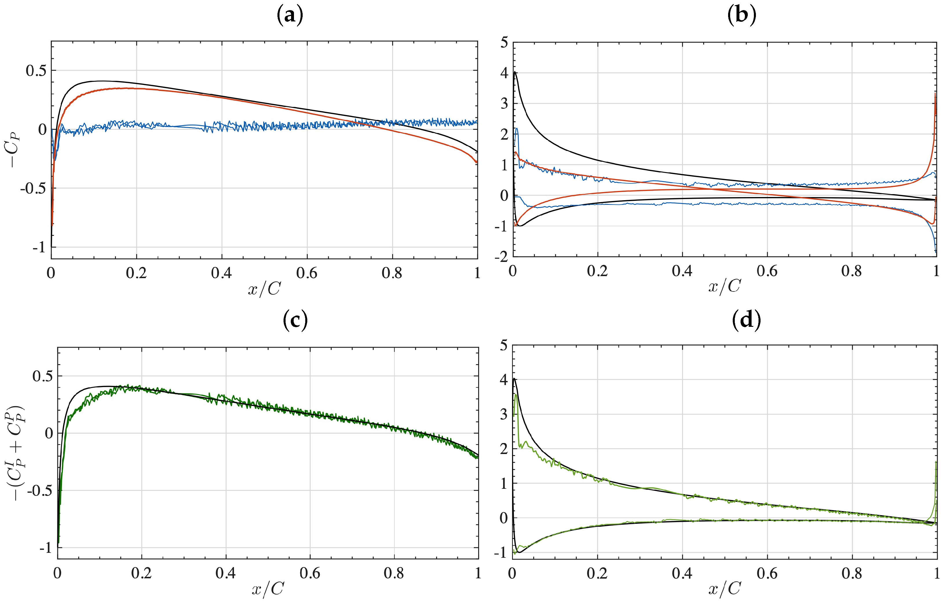
 )
,
()
,
, and ()
.; compared to: (⋄) Xfoil results and measurements by [43] for Re = , for rough (—) and smooth (- - -) foils, and [44] at Re = , for a smooth foil (– - –).
)
,
()
,
, and ()
.; compared to: (⋄) Xfoil results and measurements by [43] for Re = , for rough (—) and smooth (- - -) foils, and [44] at Re = , for a smooth foil (– - –).
)
,
()
,
, and ()
.; compared to: (⋄) Xfoil results and measurements by [43] for Re = , for rough (—) and smooth (- - -) foils, and [44] at Re = , for a smooth foil (– - –).
)
,
()
,
, and ()
.; compared to: (⋄) Xfoil results and measurements by [43] for Re = , for rough (—) and smooth (- - -) foils, and [44] at Re = , for a smooth foil (– - –).
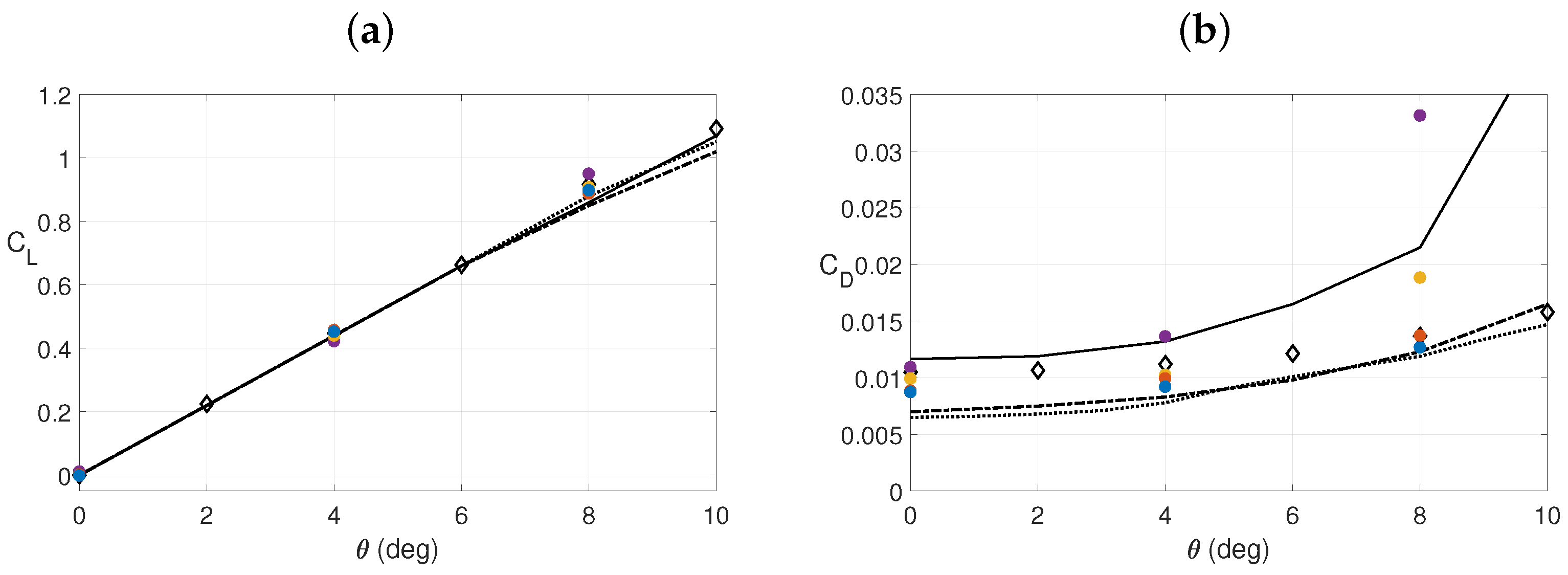
 ) , (
) , ( ), , and (
 ) , at angles of attack: (a) and (b) , compared to () Xfoil results.
) , (), , and () , at angles of attack: (a) and (b) , compared to () Xfoil results.
) , at angles of attack: (a) and (b) , compared to () Xfoil results.
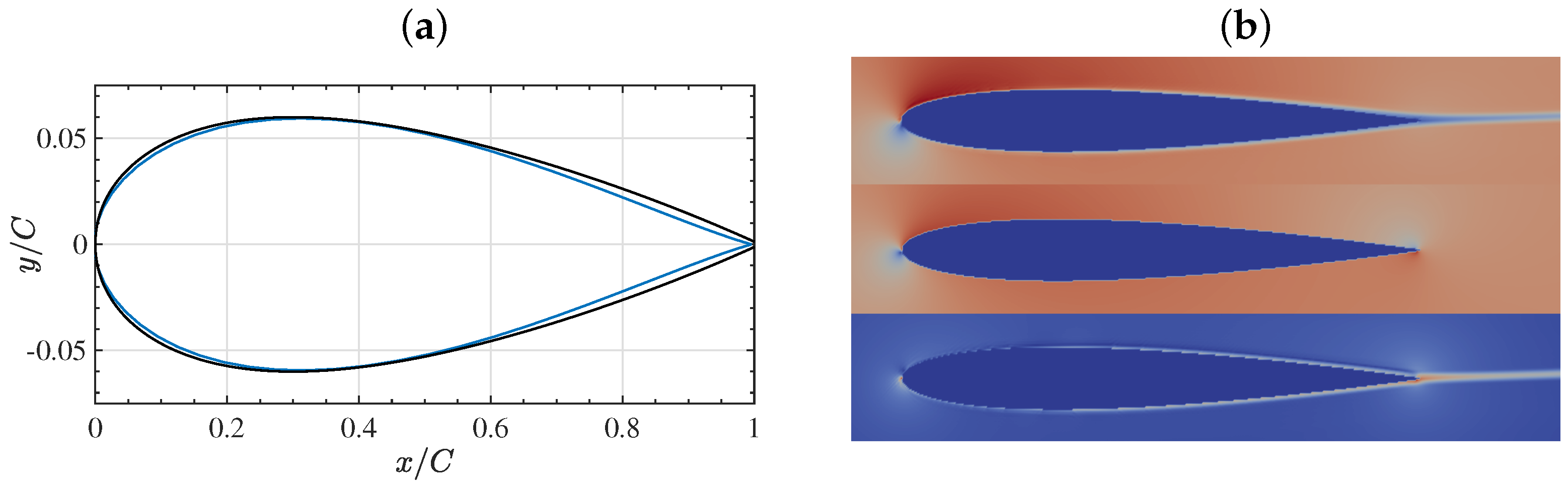
) , (), , and () , at angles of attack: (a) and (b) , compared to () Xfoil results. ), used to compute the potential (inviscid) flow component of the flow around the NACA-0012 foil profile (—-) in the pLBM. (b) Module of flow velocity calculated with the pLBM at steady state, for and : (top) total velocity, ; (middle) inviscid velocity, ; and (bottom) perturbation velocity, .
), used to compute the potential (inviscid) flow component of the flow around the NACA-0012 foil profile (—-) in the pLBM. (b) Module of flow velocity calculated with the pLBM at steady state, for and : (top) total velocity, ; (middle) inviscid velocity, ; and (bottom) perturbation velocity, .
), used to compute the potential (inviscid) flow component of the flow around the NACA-0012 foil profile (—-) in the pLBM. (b) Module of flow velocity calculated with the pLBM at steady state, for and : (top) total velocity, ; (middle) inviscid velocity, ; and (bottom) perturbation velocity, . ),
()
,
(),
()
. Xfoil simulation results are plotted as black diamonds (⋄), the measurements of [43] for Re = for a rough foil (—), and smooth foil (- - -), and the measurements of [44] at Re = for a smooth foil (– - –).
),
()
,
(),
()
. Xfoil simulation results are plotted as black diamonds (⋄), the measurements of [43] for Re = for a rough foil (—), and smooth foil (- - -), and the measurements of [44] at Re = for a smooth foil (– - –).
),
()
,
(),
()
. Xfoil simulation results are plotted as black diamonds (⋄), the measurements of [43] for Re = for a rough foil (—), and smooth foil (- - -), and the measurements of [44] at Re = for a smooth foil (– - –).
),
()
,
(),
()
. Xfoil simulation results are plotted as black diamonds (⋄), the measurements of [43] for Re = for a rough foil (—), and smooth foil (- - -), and the measurements of [44] at Re = for a smooth foil (– - –). )/ (), and (c,d) total coefficient, (
 ).
)/ (), and (c,d) total coefficient, ().
).
)/ (), and (c,d) total coefficient, ().

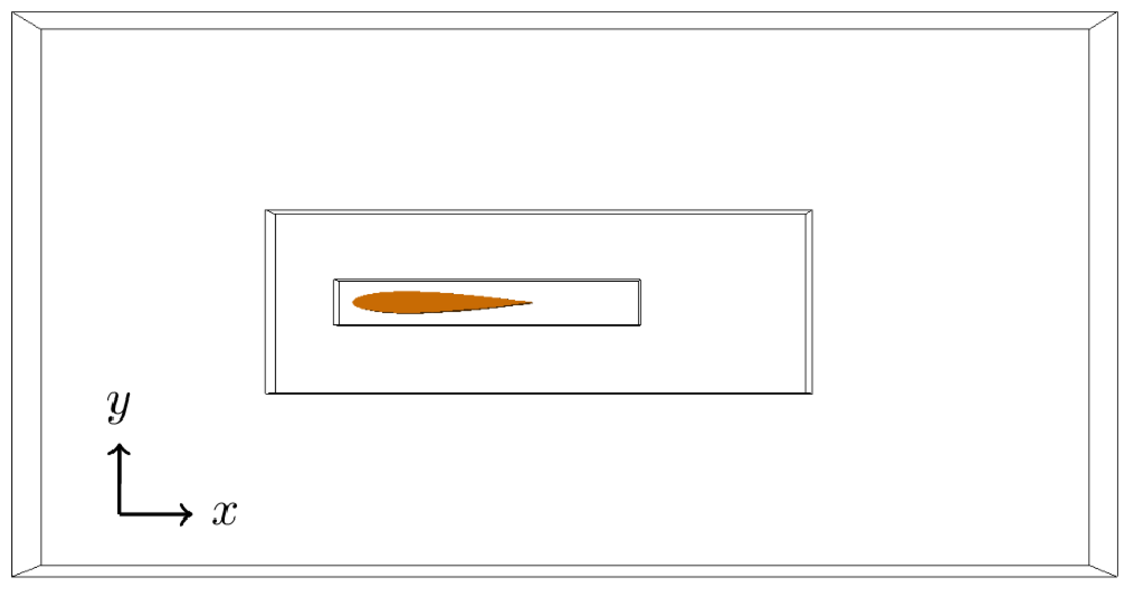
| Grid | Min. Extent | Dimensions | Nesting |
|---|---|---|---|
| Ratio | |||
| 0 | (−23.7 −30.0 −0.3) | (72.0, 60.0, 0.8) | 32 |
| 1 | (−1.85 −1.5 −0.1) | (6.0, 3.0, 0.4) | 8 |
| 2 | (−0.45 −0.25 0.0) | (3.0, 1.0, 0.25) | 2 |
| 3 | (−0.1 −0.125 0.025) | (1.7, 0.25, 0.2) | 1 |
Publisher’s Note: MDPI stays neutral with regard to jurisdictional claims in published maps and institutional affiliations. |
© 2022 by the authors. Licensee MDPI, Basel, Switzerland. This article is an open access article distributed under the terms and conditions of the Creative Commons Attribution (CC BY) license (https://creativecommons.org/licenses/by/4.0/).
Share and Cite
O’Reilly, C.M.; Grilli, S.T.; Janßen, C.F.; Dahl, J.M.; Harris, J.C. Hybrid Lattice-Boltzmann-Potential Flow Simulations of Turbulent Flow around Submerged Structures. J. Mar. Sci. Eng. 2022, 10, 1651. https://doi.org/10.3390/jmse10111651
O’Reilly CM, Grilli ST, Janßen CF, Dahl JM, Harris JC. Hybrid Lattice-Boltzmann-Potential Flow Simulations of Turbulent Flow around Submerged Structures. Journal of Marine Science and Engineering. 2022; 10(11):1651. https://doi.org/10.3390/jmse10111651
Chicago/Turabian StyleO’Reilly, Christopher M., Stephan T. Grilli, Christian F. Janßen, Jason M. Dahl, and Jeffrey C. Harris. 2022. "Hybrid Lattice-Boltzmann-Potential Flow Simulations of Turbulent Flow around Submerged Structures" Journal of Marine Science and Engineering 10, no. 11: 1651. https://doi.org/10.3390/jmse10111651