Hyperparameter Optimization for the LSTM Method of AUV Model Identification Based on Q-Learning

Abstract

An accurate mathematical model is a basis for controlling and estimating the state of an Autonomous underwater vehicle (AUV) system, so how to improve its accuracy is a fundamental problem in the field of automatic control. However, AUV systems are complex, uncertain, and highly non-linear, and it is not easy to obtain through traditional modeling methods. We fit an accurate dynamic AUV model in this study using the long short-term memory (LSTM) neural network approach. As hyper-parameter values have a significant impact on LSTM performance, it is important to select the optimal combination of hyper-parameters. The present research uses the improved Q-learning reinforcement learning algorithm to achieve this aim by improving its recognition accuracy on the verification dataset. To improve the efficiency of action exploration, we improve the Q-learning algorithm and choose the optimal initial state according to the Q table in each round of learning. It can effectively avoid the ineffective exploration of the reinforcement learning agent between the poor-performing hyperparameter combinations. Finally, the experiments based on simulated or actual trial data demonstrate that the proposed model identification method can effectively predict kinematic motion data, and more importantly, the modified Q-Learning approach can optimize the network hyperparameters in the LSTM.

1. Introduction

The ocean occupies most of the earth’s surface and is an important area for commercial activities, scientific research, and resource extraction, and its impact is critical to all aspects [1,2]. Over the past half-century, oceanographic research has shown that the oceans and seafloor are critical to understanding the planet. Exploring the marine environment provides valuable knowledge for many areas of science and engineering. AUVs have been widely used in marine engineering due to their unique advantages. Autonomous underwater vehicles (AUVs) equipped with various sensors have broad applications in scientific, military, and commercial missions, such as deep-sea exploration, cable/pipe tracking, feature tracking, and more [3].

AUVs are complex nonlinear coupled systems, and it is challenging to model them accurately [4,5]. Therefore, studying the non-linear mechanism of AUV systems and finding mathematical methods that can accurately express them have become the focus of AUV research, which has essential educational and economic value [6,7,8,9]. Neural network models have recently been widely used in AUV system model identification. In the identification networks, recursive structures are adapted to acquire dynamic information and improve the communication between neurons [10]. The experimental results show that the method can fit the AUV system. The weight values of the network were tuned using a hybrid algorithm of the genetic algorithm (GA) and the error backpropagation algorithm (BP) [11]. Moreover, the neural network with the hybrid learning algorithm improves the learning speed of convergence and identification accuracy. An approximation of the lumped disturbance and estimation of the parametric uncertainty is achieved by a dynamic neural network [12]. The Bayesian network is used to construct a state observer for robot control when both the actuator and sensor models are used [13]. A multi-scale attention-based long short-term memory (LSTM) model is adopted to identify the ship’s non-linear model under different ocean conditions. The experiment results show that the LSTM model has higher prediction accuracy than the traditional support vector regression (SVR) and radial basis function (RBF) model [14]. Ref. [15] also shows that the LSTM method has a high quality of time-series prediction and has important practical applications. Therefore, this study uses an LSTM neural network approach for AUV system identification.

Neural networks have good non-linear mapping ability and have been widely used in system identification, especially in non-linear systems [16,17,18]. The value of the neural network hyperparameters can significantly affect its performance [19]. However, its value has no theoretical guidance, and different systems often require different values. Therefore, it is of great practical significance to study a method for automatic optimization of hyperparameters of system identification algorithm [20,21].

In response to the above problems, some optimization methods of neural network model structure based on reinforcement learning have been proposed. Meta-modeling based on reinforcement learning enables automated generation of high-performing convolutional neural network (CNN) architectures for a given learning task [22]. A novel multi-objective reinforcement learning method is proposed for hyperparameter optimization to solve the limitations in the actual environment, such as latency and CPU utilization [23]. A context-based meta-RL approach is used to maximize the accuracy of the validation set [24]. It can tackle the data-inefficiency problem of hyperparameter optimization. The above methods have proved the effectiveness of reinforcement learning in hyperparameter optimization. If the hyperparameter optimization problem of a neural network is regarded as a reinforcement learning problem of continuous state-action space, such as deep Q network (DQN) [25] or proximal policy optimization (PPO) [26], the algorithm needs to go through hundreds or even thousands of times of learning to ensure convergence. When the computing resources are minimal, it is not suitable for the situation where the search space of parameters is ample or the performance evaluation of the algorithm is very expensive. Therefore, the Q-learning [27] algorithm is selected in this paper to solve the hyperparameter optimization problem of the LSTM neural network.

Our main objective in this paper is to identify the AUV model and optimize hyperparameters using an improved Q-learning LSTM neural network method. The main contributions of this paper lie in the following three points: (1) We adopt the LSTM method to identify the AUV dynamic model and conduct an in-depth analysis of its principle; (2) Reinforcement learning framework to solve the hyperparameter optimization problem of the LSTM method; (3) The method’s effectiveness in this paper is verified by verifying the actual AUV dataset.

The rest of the paper is organized as follows: Section 2 provides the AUV’s hydrodynamic model and force analysis. Section 3 describes in details of the proposed method. The experimental results are presented and discussed in Section 4. Finally, Section 5 gives the main conclusions and discusses future work.

2. AUV Model Analysis

2.1. AUV Hydrodynamic Model

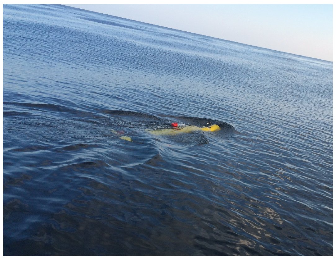
This research focuses on the "Sailfish" 210 AUV developed by the Underwater Vehicle Laboratory of Ocean University of China (Qingdao, China), as shown in Figure 1. The cabin structure comprises four sections: the bow, the navigation cabin, the electronic energy cabin, and the propulsion system cabin. A unified electrical and mechanical interface is used between the cabins, which is beneficial for us to configure different loads for the AUV for different task requirements. The bow is generally equipped with an underwater acoustic communication machine; the navigation cabin includes attitude and heading reference system (AHRS), global positioning system (GPS), doppler velocity log (DVL), etc. The electronic energy cabin includes batteries, industrial computer systems, etc.; the propulsion system cabin mainly includes steering gear and thruster motors. The experiments carried out in this paper are based on the "Sailfish" 210 AUV platform, which has a maximum speed of 5 kn (2.5 m/s). The parameters are shown in

Table 1. The parameters of the AUV model.

Definition	Symbol	Unit	Numerical Value
Mass	m	kg	73
Diameter	d	mm	210
Length	l	m	2.2
Center of gravity	$x_G,y_G,z_G$	mm	$0,0,0.02$
Center of buoyancy	$x_B,y_B,z_B$	mm	$0,0,0$
Moment of inertia	$I_x,I_y,I_z$	kg·m${}^2$	$0.4,24.5,24.5$

.

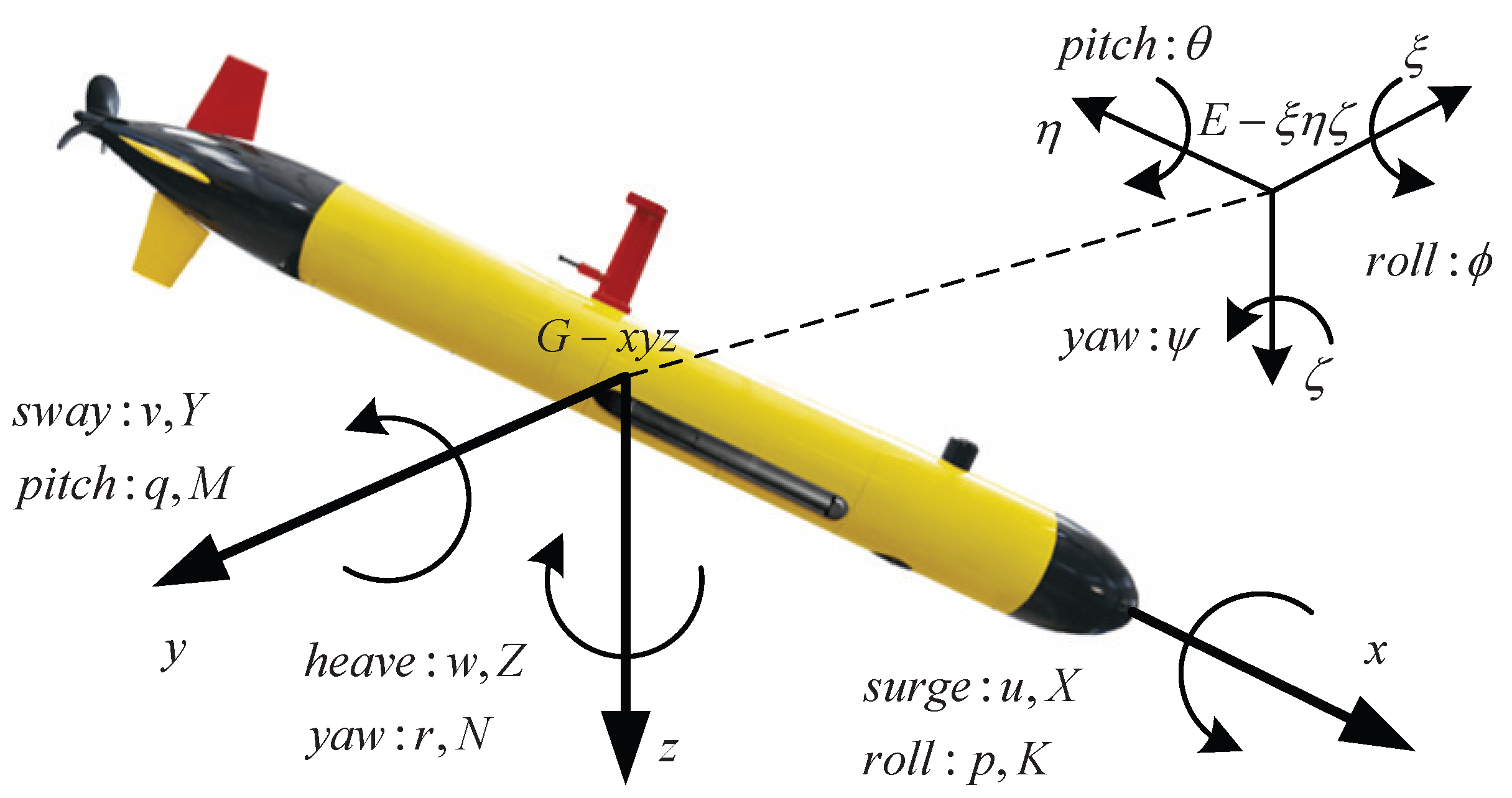
The general motion of the AUV was described with two coordinate systems, body-fixed reference frame $(G-xyz)$ and earth-fixed reference frame $(E-\xi \eta \zeta )$ [28]. AUV translational and rotational motions are described in six degrees of freedom (6DOF) as follows:

$$\begin{array}{c}\eta ={\left[{\eta }_1^T{\eta }_2^T\right]}^T,{\eta }_1={\left[\eta \xi \zeta \right]}^T,{\eta }_2={\left[\varphi \theta \psi \right]}^T\hfill \\ v={\left[v_1^T{v}_2^T\right]}^T,v_1={\left[uvw\right]}^T,v_2={\left[pqr\right]}^T\hfill \\ \tau ={\left[{\tau }_1^T{\tau }_2^T\right]}^T,{\tau }_1={\left[XYZ\right]}^T,{\tau }_2={\left[KMN\right]}^T\hfill \end{array}$$

(1)

where ${\eta }_1$ and ${\eta }_2$ refer to the position and orientation of the AUV with respect to the earth-fixed reference frame, $\upsilon$ denotes the translational and rotational speeds with respect to the body-fixed reference frame, ${\tau }_1$ and ${\tau }_2$ refer to the external forces and moments with respect to the body-fixed reference frame. A diagram of the AUV coordinate system is shown in Figure 1.

Translational velocities $\left[uvw\right]$ are converted from linear velocities $\left[\dot{\xi }\dot{\eta }\dot{\zeta }\right]$ by $T_1$:

$$T_1=\left[\begin{array}{ccc}cos\psi cos\theta & cos\psi sin\theta sin\varphi -sin\psi cos\varphi & cos\psi sin\theta cos\varphi +sin\psi sin\varphi \\ sin\psi cos\theta & sin\psi sin\theta sin\varphi +cos\psi cos\varphi & sin\psi sin\theta cos\varphi -cos\psi sin\varphi \\ -sin\theta & cos\theta sin\varphi & cos\theta cos\varphi \end{array}\right]$$

(2)

Then,

$$\left[\begin{array}{c}\begin{array}{c}\dot{\xi }\\ \dot{\eta }\end{array}\\ \dot{\zeta }\end{array}\right]=T_1\left[\begin{array}{c}u\\ v\\ w\end{array}\right]$$

(3)

The angular rates $\left[\dot{\varphi }\dot{\theta }\dot{\psi }\right]$ are converted to the rotational velocities $\left[pqr\right]$ by $T_2$:

$$T_2=\left[\begin{array}{ccc}1& sin\varphi tan\theta & cos\varphi tan\theta \\ 0& cos\varphi & -sin\varphi \\ 0& sin\varphi /cos\theta & cos\varphi /cos\theta \end{array}\right]$$

(4)

Thus,

$$\left[\begin{array}{c}\begin{array}{c}\dot{\varphi }\\ \dot{\theta }\end{array}\\ \dot{\psi }\end{array}\right]=T_2\left[\begin{array}{c}p\\ q\\ r\end{array}\right]$$

(5)

The general motion is described in $(G-xyz)$ by Equation (6), where the first three equations describe the translation and the last three describe rotation:

$$\left\{\begin{array}{c}m[(\dot{u}-vr+wq)-x_G(q^2+r^2)+y_G(pq-\dot{r})+z_G(pr+\dot{q})]=\sum X\\ m[(\dot{v}-wp+ur)-y_G(r^2+p^2)+z_G(qr-\dot{p})+x_G(qp+\dot{r})]=\sum Y\\ m[(\dot{w}-uq+vq)-z_G(p^2+q^2)+x_G(rp-\dot{q})+y_G(rq+\dot{p})]=\sum Z\\ I_x\dot{p}+(I_z-I_y)qr+m[y_G(\dot{w}+pv-qu)-z_G(\dot{v}+ru-pw)]=\sum K\\ I_y\dot{q}+(I_x-I_z)rp+m[z_G(\dot{u}+wq-vr)-x_G(\dot{w}+pv-uq)]=\sum M\\ I_z\dot{r}+(I_y-I_x)pq+m[x_G(\dot{r}+ur-pw)-y_G(\dot{u}+qw-vr)]=\sum N\end{array}\right.$$

(6)

where:

m: AUV mass.

$x_G,y_G,z_G$: the position of centre gravity of the AUV.

$I_x,I_y,I_z$: the moment of inertia of the AUV.

$u,v,w$: velocities along the x-axis, y-axis, and z-axis of the AUV.

$p,q,r$: roll angular velocity, pitch angular velocity and yaw angular velocity.

$\dot{u},\dot{v},\dot{w},\dot{p},\dot{q},\dot{r}$: linear acceleration and angular acceleration.

$\sum X,\sum Y,\sum Z,\sum K,\sum M,\sum N$: external force and moment.

2.2. The Dynamical Principles AUV Model Identification

The dynamic model mathematically describes the essential law of the interaction between the AUV and the environment, which can well reflect the state transition of the AUV under the action of force. This paper will realize the AUV model identification based on the dynamic model. The external force (moment) exerted on the AUV mainly includes gravity and buoyancy, hydrodynamic force, rudder force, thrust force, etc. [29]. The force analysis and model identification principle are detailed below.

2.2.1. The Static Force

The static force of the AUV is generated by the gravity P and buoyancy B. The center of buoyancy and center of gravity coordinates in the body-fixed frame are $(0,0,0)$ and $(0,0,z_e)$. The component of the static force in the earth-fixed frame is $(0,0,P-B)$, which can be obtained by converting it to the motion coordinate system by Equation (7):

$$\left\{\begin{array}{c}X=-(P-B)sin\left(\theta \right)\hfill \\ Y=-(P-B)cos\theta sin\varphi \hfill \\ Z=-(P-B)cos\theta cos\varphi \hfill \\ K=-phcos\theta sin\varphi \hfill \\ M=-phsin\theta \hfill \\ N=0\hfill \end{array}\right.$$

(7)

where p is the underwater full displacement of AUV and h represents the depth of AUV.

2.2.2. Hydrodynamic Force

The hydrodynamic forces of AUV are usually divided into inertial hydrodynamic forces and viscous hydrodynamic forces, and the interaction between the two is ignored. In infinitely deep, wide and still water, the hydrodynamic forces of the AUV depend only on its motion and is a function of motion parameters $u,v,w,p,q,r,\dot{u},\dot{v},\dot{w},\dot{p},\dot{q},\dot{r}$. According to the idea of Taylor expansion, the hydrodynamic forces $(X_H,Y_H,Z_H)$ and the moments $(K_H,M_H,N_H)$ are expanded to obtain the expression of the hydrodynamic forces:

$$\begin{array}{c}{X}_H=[X_{qq}{q}^2+X_{rr}{r}^2+X_{rp}rp]+[X_{\dot{u}}\dot{u}+X_{vr}vr+X_{wq}wq]+[X_{u\left|u\right|}u\left|u\right|+\hfill \\ X_{vv}{v}^2+X_{ww}{w}^2]\hfill \\ Y_H=[Y_{\dot{r}}\dot{r}+Y_{qr}qr+Y_{\dot{p}}\dot{p}+Y_{pq}pq+Y_{p\left|p\right|}p\left|p\right|]+[Y_{\dot{v}}\dot{v}+Y_{vq}vq+Y_{wr}wr+\hfill \\ Y_{wp}wp]+[Y_{r}ur+Y_{v\left|r\right|}\frac{v}{\left|v\right|}{\left(v^2+w^2\right)}^{\raisebox{1ex}{$1$}\!\left/ \!\raisebox{-1ex}{$2$}\right.}\left|r\right|+Y_{p}up]+[Y_0{u}^2+Y_{v}uv+\hfill \\ Y_{v\left|v\right|}v{\left(v^2+w^2\right)}^{\raisebox{1ex}{$1$}\!\left/ \!\raisebox{-1ex}{$2$}\right.}]+Y_{vw}vw\hfill \\ Z_H=[Z_{\dot{q}}\dot{q}+Z_{rr}{r}^2+Z_{pp}{p}^2+Z_{rp}rp]+[Z_{\dot{w}}\dot{w}+Z_{vr}vr+Z_{vp}vp]+[Z_{q}uq+\hfill \\ Z_{w\left|q\right|}\frac{w}{\left|w\right|}{\left(v^2+w^2\right)}^{\raisebox{1ex}{$1$}\!\left/ \!\raisebox{-1ex}{$2$}\right.}\left|q\right|]+[Z_0{u}^2+Z_{w}uw+Z_{w\left|w\right|}w{\left(v^2+w^2\right)}^{\raisebox{1ex}{$1$}\!\left/ \!\raisebox{-1ex}{$2$}\right.}]+\hfill \\ [Z_{\left|w\right|}u\left|w\right|+Z_{ww}\left|w{\left(v^2+w^2\right)}^{\raisebox{1ex}{$1$}\!\left/ \!\raisebox{-1ex}{$2$}\right.}\right|]+Z_{vv}{v}^2\hfill \\ K_H=[K_{\dot{p}}\dot{p}+K_{\dot{r}}\dot{r}+K_{qr}qr+K_{pq}pq+K_{p\left|p\right|}p\left|p\right|]+[K_{p}up+K_{r}ur+K_{\dot{v}}\dot{v}]+\hfill \\ [K_{vq}vq+K_{wp}wp+K_{wr}wr]+[K_0{u}^2+K_{v}uv+K_{v\left|v\right|}v\left|v\right|{\left(v^2+w^2\right)}^{\raisebox{1ex}{$1$}\!\left/ \!\raisebox{-1ex}{$2$}\right.}]+\hfill \\ K_{vw}vw\hfill \\ M_H=[M_{\dot{q}}\dot{q}+M_{rr}{r}^2+M_{q\left|q\right|}q\left|q\right|+M_{pp}{p}^2+M_{rp}rp]+[M_{\dot{w}}\dot{w}+M_{vr}vr+\hfill \\ M_{vp}vp]+[M_{q}uq+M_{\left|w\right|q}q{\left(v^2+w^2\right)}^{\raisebox{1ex}{$1$}\!\left/ \!\raisebox{-1ex}{$2$}\right.}]+[M_0{u}^2+M_{w}uw+\hfill \\ M_{w\left|w\right|}w{\left(v^2+w^2\right)}^{\raisebox{1ex}{$1$}\!\left/ \!\raisebox{-1ex}{$2$}\right.}]+[M_{\left|w\right|}u\left|w\right|+M_{ww}\left|w{\left(v^2+w^2\right)}^{\raisebox{1ex}{$1$}\!\left/ \!\raisebox{-1ex}{$2$}\right.}\right|]+M_{vv}{v}^2\hfill \\ N_H=[N_{\dot{r}}\dot{r}+N_{qr}qr+N_{r\left|r\right|}r\left|r\right|+N_{\dot{p}}\dot{p}+N_{pq}pq]+[N_{\dot{v}}\dot{v}+N_{wr}wr+N_{vq}vq+\hfill \\ N_{wp}wp]+[N_{r}ur+N_{\left|v\right|r}r{\left(v^2+w^2\right)}^{\raisebox{1ex}{$1$}\!\left/ \!\raisebox{-1ex}{$2$}\right.}+N_{p}up]+[N_0{u}^2+N_{v}uv+\hfill \\ N_{v\left|v\right|}v{\left(v^2+w^2\right)}^{\raisebox{1ex}{$1$}\!\left/ \!\raisebox{-1ex}{$2$}\right.}]+N_{vw}vw\hfill \end{array}$$

(8)

2.2.3. Thrust

The thrust generated by the propeller is calculated as follows:

$$X_T=(1-t)\rho n^2{D}^4{K}_T$$

(9)

where r: the propeller rotational speed; D: the propeller diameter; t: thrust derating factor; $\rho$: the water density; and $K_T$: dimensionless thrust coefficient. $K_T$ is a function related to the advance ratio $J=\frac{u(1-w)}{nD}$, which can be approximated as:

$$K_T=k_0+k_{1}J+k_2{J}^2$$

(10)

where $k_0,k_1,k_2$ are a constant coefficients.

$n=\frac{u(1-w)}{DJ}$ can be obtained from the advance ratio formula, and the relevant variables are substituted into Equation (9), the functional relationship between thrust and speed can be obtained with the following equation:

$$X_T=\frac{1}{2}\rho L^2{u}^2(a_T+b_T+c_T)$$

(11)

where L is the body length, $a_T=\mu k_2$, $b_T=\mu k_1/\phantom{\mu k_{1}J}J$, $c_T=\mu k_0/\phantom{\mu k_0{J}^2}{J}^2$, $\mu =2(1-t){(1-w)}^2{D}^2/\phantom{2(1-t){(1-w)}^2{D}^2{L}^2}{L}^2$.

2.2.4. Rudder Force

This paper discusses the underactuated underwater robot, whose rudder force comes from a pair of horizontal and vertical rudders mounted on its tail. When the rudder moves at speed V and angle of attack $\alpha$, it will be subjected to two parts of force: lift force perpendicular to the direction of the water flow, and the resistance along the direction of the water flow, the calculation formula is as follows:

$$\begin{array}{c}L=\frac{1}{2}{C}_L\rho A_R{V}^2\hfill \\ D=\frac{1}{2}{C}_D\rho A_R{V}^2\hfill \end{array}$$

(12)

where $C_L$ is the lift coefficient, $C_D$ is the drag coefficient, and $A_R$ is the cross-sectional area of the rudder.

2.2.5. The Principle of Identification

$F_{else}={[X_{else},Y_{else},Z_{else},K_{else},M_{else},N_{else}]}^T$ is used to represent static force, thrust force, rudder force, and disturbance force. Then, using the superposition principle, we can obtain the AUV force expression:

$$F=F_H+F_{else}$$

(13)

Bring Equation (13) into Equation (6), and simplify the equation of motion, we can obtain:

$$E\dot{X}=F_{vis}+F_{else}$$

(14)

where:

$$X={\left[u,v,w,p,q,r\right]}^T$$

(15)

$$E=\left[\begin{array}{cccccc}m-X_{\dot{u}}& 0& 0& 0& m{z}_G& -m{y}_G\\ 0& m-Y_{\dot{v}}& 0& m{z}_g& 0& m{x}_G-Y_{\dot{r}}\\ 0& 0& m-Z_{\dot{w}}& m{y}_G& -m{x}_G-Z_{\dot{q}}& 0\\ 0& -m{z}_G& m{y}_G& I_x-K_{\dot{p}}& 0& 0\\ m{z}_G& 0& -m{x}_G-M_{\dot{w}}& 0& I_y-M_{\dot{q}}& 0\\ -m{y}_G& m{x}_G-N_{\dot{v}}& 0& 0& 0& I_z-N_{\dot{r}}\end{array}\right]$$

(16)

$F_{vis}={\left[X_{vis},Y_{vis},Z_{vis},K_{vis},M_{vis},N_{vis}\right]}^T$ is non-inertial hydrodynamic force.

It can be seen from the above analysis that the acceleration of the AUV is recorded as the combined action of the non-inertial hydrodynamic force and other forces except the hydrodynamic force, denoted as $\dot{X}=f(u,v,w,p,q,r,n,{\delta }_r,{\delta }_s)$. Further, the acceleration results from the non-inertial hydrodynamic force $F_{vis}=f_H(u,v,w,p,q,r)$, the thrust force $F_T=f_T(u,n)$, and the rudder force $F_{L/D}=f_{\delta }(u,{\delta }_r,{\delta }_s)$.

Based on the above analysis of the AUV model, the AUV states are denoted as $X_t=[x,y,z,\varphi ,\theta ,\psi ,u,v,w,p,q,r]$, then the state changes can be expressed as $\Delta X_t=f_1(\varphi ,\theta ,\psi ,u,v,w,p,q,r,n,{\delta }_r,{\delta }_s)$. The historical data of AUV implies the causal relationship of its dynamic model and has the characteristics of a hidden Markov model, which can be used to build an AUV data-driven model.

3. AUV Model Identification Method

AUV system identification is essentially a mathematical modeling method. Its primary purpose is to build its mathematical model, which can be used in many aspects, such as controller involvement, system prediction, and system simulation. We can see from the above that the AUV system is a complex and uncertain, highly nonlinear system, and it is not easy to obtain an accurate dynamic model. We aim at this problem by adopting a data-driven model identification method based on LSTM neural network. Further, the Q method is used to optimize its hyperparameters to improve the learning efficiency of the LSTM neural network.

3.1. Fundamentals of System Identification

Identification based on a neural network means that the neural network is directly used to learn the mapping relationship between input and output. The learning criterion minimizes the error between the network’s output and the system’s actual output. From the above, the goal of learning is to minimize the objective function of error [30], which is as follows:

$$E=\frac{1}{2}{(y\left(t\right)-y_n\left(t\right))}^2$$

(17)

where, $y_n\left(t\right)$ is the output of the neural network at time t, and $y\left(t\right)$ is the actual output of the system at time t. Neural networks can fit any function with arbitrary precision. In principle, the desired output will be obtained as long as there is enough training data and input.

Since the environment is full of time-series information, the information before and after them is related to a certain extent. For example, AUV’s position and attitude data are all data sequences that change with time. Additionally, the LSTM [31,32] is good at processing this kind of data information. Its basic structure is shown in Figure 2.

The network structure introduces a cell state which contains all the information at the last moment. When new information is encountered, a series of operations will be taken to choose between the old and new information. Coupled with the introduced “memory-forgetting” mechanism, the processing of long-term series data can be realized. The structure mainly includes input, forget, and output gates. The input are $h_{t-1}$ and $x_t$, the output is $h_t$, and the cell states are $c_{t-1}$ and $c_t$.

The forget gate controls the time dependence and effects of previous inputs and determines which states are remembered or forgotten. The output of the forget gate is:

$$o_f=\sigma (w_f{x}_t+u_f{h}_{t-1})C_{t-1}$$

(18)

The input gate is also called the selection memory stage. It is to decide the degree of consideration for the current moment. The calculations for each part are as follows:

$$\left\{\begin{array}{c}{i}_t=\sigma (w_i{x}_t+u_i{h}_{t-1})\hfill \\ {C_t}^{\prime }=tanh(w_c{x}_t+u_c{h}_{t-1})\hfill \\ C_t=f_t{C}_{t-1}+{C_t}^{\prime }{i}_t\hfill \end{array}\right.$$

(19)

The output gate determines the final output information. The computational procedure is summarized as follows.

$$\left\{\begin{array}{c}{O}_t=\sigma (w_o{x}_t+u_o{h}_{t-1})\hfill \\ h_t=O_{t}tanh\left(C_t\right)\hfill \end{array}\right.$$

(20)

The above is the basic principle of the neural network LSTM, which uses the gated state to selectively memorize the input information to meet memory needs, while forgetting the long-term sequence information.

3.2. Identification Principle and Process

After the actual test of AUV, we can obtain the dataset required for model identification. After removing the invalid data, an input and output model is established according to the navigation control instruction information of the AUV and its posture information. According to Equation (14), we can obtain:

$$\dot{x}=\frac{dx}{dt}=\left[\begin{array}{c}{x}_4\\ x_5\\ x_6\\ E_1{F}_1\\ E_2{F}_2\\ \begin{array}{c}{E}_3{F}_3\hfill \\ \begin{array}{c}{x}_{10}\\ x_{11}\\ x_{12}\\ E_4{F}_4\\ E_5{F}_5\\ E_6{F}_6\end{array}\hfill \end{array}\end{array}\right]$$

(21)

where, $\left\{\begin{array}{c}{x}_1=x,x_2=y,x_3=z,x_4=u,x_5=v,x_6=w,x_7=\varphi ,x_8=\theta ,x_9=\psi ,\\ x_{10}=p,x_{11}=q,x_{12}=r\\ F=F(\varphi ,\theta ,\psi ,u,v,w,p,q,r,n,{\delta }_r,{\delta }_s)\end{array}\right.$. The subscripts of the matrices $E_n$ and $F_n$ represent the row and column of the matrix, respectively. Next, the learned AUV dynamic model can be expressed as:

$$P(x_t^{\prime },u_t^{\prime }):(x_t^{\prime },u_t^{\prime })\to (y_{t+1}^{\prime }-y_t^{\prime })=\Delta y_t^{\prime }$$

(22)

where $u_t^{\prime }$ is comprised of the thruster command $n_t$ and rudder angle commands $({\delta }_{r_t},{\delta }_{s_t})$.

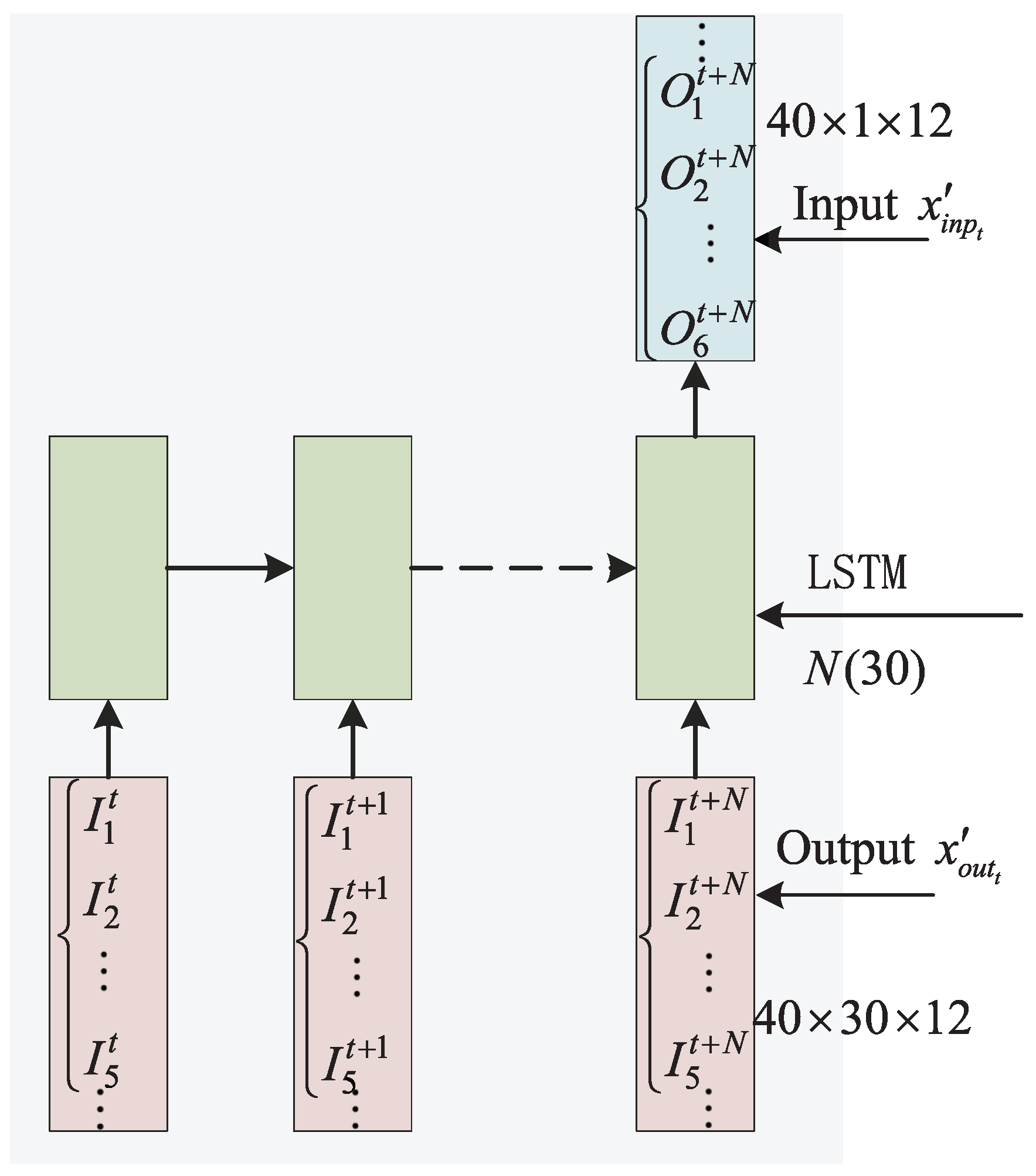
The structure of the LSTM-based AUV model is shown in Figure 3. The input elements of the input layer is $x_{in{p}_t}^{\prime }=[x_t^{\prime },u_t^{\prime }]$, and the output of neural network is $x_{ou{t}_t}^{\prime }=[\Delta y_t^{\prime }]$. The attitude and speed information of the next moment can be obtained by using the control instruction, attitude and speed information of 20 sets of time-series data. The learned model can be optimized according to the set loss function. More details of network architectures are described below.

To avoid inconsistencies due to different relative scale sizes of different features, we normalize the data as follows:

$$f:x\to x^{\prime }=\frac{x-x_{min}}{x_{max}-x_{min}}$$

(23)

where $x,x^{\prime }\in R$, $x_{min}=min\left(x\right)$, $x_{max}=max\left(x\right)$.

Model evaluation criteria are mainly used to evaluate the accuracy of the recognition model. In this study, the mean square error between the output of the neural network and the actual output is used as the evaluation index, as follows:

$$MSE=\frac{1}{N}\sum _{n=1}^N{\left[d\right(n)-y(n\left)\right]}^2$$

(24)

where $d\left(n\right)$ is the output of the neural network, $y\left(n\right)$ is the system’s actual output, and N is the number of datasets calculated at one time.

For the system identification of the AUV in this study, the model is trained by minimizing the error $M=\frac{1}{\left|D\right|}{\displaystyle \sum _{(I,\Delta y^{\prime })\in D}}\frac{1}{2}\left|\right|(\Delta y_t^{\prime }-O)|{|}^2$, where $O=P\left(I\right)$, the training dataset D consists of input–output training pairs $I:(x^{\prime },u^{\prime })\to O:(\Delta y)$. The multi-step error is adopted to test the effectiveness of the learned dynamic model, as shown in Equation (25).

$$M^H=\frac{1}{|D_H|}\sum _{(O^{\prime },{u^{\prime }}_t,\Delta y^{\prime })\in D_H}\frac{1}{H}\sum _{h=1}^H\frac{1}{2}\left|\right|(\Delta y-P\left((O_{4-12}^{\prime },u_t^{\prime })\right))|{|}^2$$

(25)

where $O_{4-12}^{\prime }$ represents the desired input data $(\varphi ,\theta ,\psi ,u,v,w,p,q,r)$ from the first four columns of the output data $O^{\prime }$ obtained in the previous step. Additionally, the training dataset $D_H$ consists of input–output data pairs $I:(O_{4-12}^{\prime },u^{\prime })\to O:(\Delta y)$. To sum up, the learned multi-step model can update the AUV state $(x,y,z,\varphi ,\theta ,\psi ,u,v,w,p,q,r)$ in a cyclic manner using only action instructions $u^{\prime }$.

3.3. Hyperparameter Optimization for Identification Algorithm

3.3.1. MDP Modeling of LSTM Hyperparameter Optimization Problems

The performance of the LSTM algorithm is highly dependent on hyperparameters. Moreover, different tasks often require different hyperparameter configurations. To achieve high-precision identification of the AUV system, we adopt reinforcement learning to optimize the hyperparameter configuration of the LSTM network.

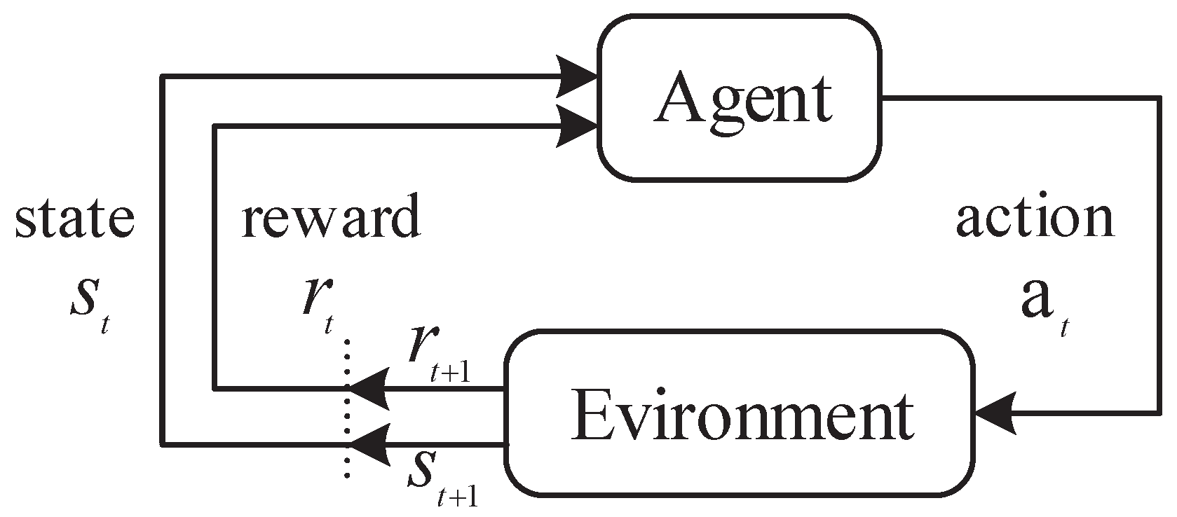
Reinforcement learning is one of the many categories of machine learning methods in which the best/suboptimal strategy is determined by interacting with dynamic environments [33]. A Markov Decision Process (MDP) includes five elements: $M=\langle S,A,R,T,\gamma \rangle$: where:

S: the set of possible states.

A: the set of actions generated by the policy.

R: reward model.

T: dynamics model, the probability of reaching the next state with the current state and action.

$\gamma$: discount factor (between 0 and 1).

Figure 4 shows the basic structure of reinforcement learning. In this way, the agent learns how to map states to actions. At time t, the agent receives state $s_t$ and produces action $a_t$, then transitions to the next state $s_{t+1}$ and obtains reward $r_t$. The process does not stop until the final condition is reached. To improve the optimization efficiency, the hyperparameter optimization of the LSTM neural network is regarded as a reinforcement learning problem with discrete state space and discrete action space. Then, the above elements are designed for this problem.

Action space: The hyperparameters to be optimized and the candidate values of each hyperparameter are determined according to the LSTM network model structure. We concentrate on the number of neurons $N_{n1}$ and $N_{n2}$ in the hidden layers, batch size $N_b$ and time step $N_{ts}$ in this study, while other settings are determined empirically. Therefore, the hyperparameters to be optimized and their candidate values are shown in

Table 2. The optimized hyperparameters and variation ranges.

Hyperparameter	Variation Range
The number of neurons (1)	$(50,100,150,200)$
The number of neurons (2)	$(50,100,150,200)$
Batch size	$(8,16,32,64)$
Time step	$(5,10,15,20)$

.

State space: In this paper, the current hyperparameter configuration a of the network is taken as the state s at time t. Then, the state space S is the same as the action space A, that is, ($N_{n1}$, $N_{n2}$, $N_b$, $N_{ts}$).

Reward: It can be seen from the previous analysis that the error of identification decreases with a decreasing output error. So we define the immediate reward as the root mean square error of test sets with Equation (26).

$$r=-\frac{1}{N_t}\sum _{n=1}^{N_t}{[d_t\left(n\right)-y_t\left(n\right)]}^2$$

(26)

where $N_t$ is the number of datasets, $d_t$, and $y_t$ present the output of network and the real output on the testing set, respectively.

3.3.2. Hyperparameter Optimization Method

The hyperparameter optimization problem of the LSTM neural network is defined as a reinforcement learning problem with discrete state space and action space. Reinforcement learning methods for value function or policy approximation through neural networks, such as DQN, are also suitable for solving reinforcement learning problems with discrete action spaces. However, this kind of algorithm needs much learning to ensure convergence, and it is not suitable for these methods when the computing resources are very limited. Thus, the Q-Learning algorithm is selected in this paper to solve the problem.

Q-Learning is a temporal difference algorithm designed to solve the reinforcement learning problem. The optimal action policy ${\pi }^{\ast }:s_t\to a_t$ can be obtained by maximizing the action value Q function $Q\left(s_t,a_t\right)$, which reflects the long-term impact of an action. The Q function is updated according to Equation (27):

$$Q\left(s_t,a_t\right)=\left(1-\alpha \right)Q\left(s_t,a_t\right)+\alpha \left[r_t+\gamma \underset{a_{t+1}}{max}Q\left(s_{t+1},a_{t+1}\right)\right]$$

(27)

where $0<\alpha <1$ is a learning rate, $0<\gamma <1$ is the discount factor.

The structure of the LSTM hyperparameter optimization method based on Q-Learning is shown in Figure 5. The hyperparameter optimization process is as follows: first, the Q-value table is initialized with zeros, and the initial hyperparameter configurations (that is, initial state $s_0$) are randomly selected in the action space. Then, the action $a_t$ is chosen according to the e-greedy selection rule. Next, we perform the new action $a_t$ and the system acquires a new state $s_{t+1}$ and reward $r_{t+1}$. Finally, the Q-value table is updated according to the formula. The round ends when the termination conditions are met.

To improve the optimization efficiency of hyperparameters, we improve the above methods. In each round of learning, in addition to randomly selecting the initial state in the first round, the agent selects the current best hyperparameter configuration as the initial state to start optimization. It can effectively avoid the ineffective exploration of the reinforcement learning agent between the poor-performing hyperparameter combinations.

3.4. Identification Algorithm

After introducing the model identification method based on LSTM and the hyperparameter optimization method based on improved Q-learning, we can obtain the complete process and framework of the method in this paper. The algorithm flow of hyperparameter optimization for the LSTM method of AUV model identification based on Q-Learning is shown in

Table 3. AUV Model Identification Algorithm.

AUV Model Identification Algorithm
Given a training datasets, including input and output datasets
do for episode in 1 to count
Network initialization: Initialize neural network hyperparameters
do for t in 1 to T
Choose optimized hyperparameters
Calculate network output
Calculate the error between the true output and the output of the network
Update neural network
Update Q table
end for
end for

.

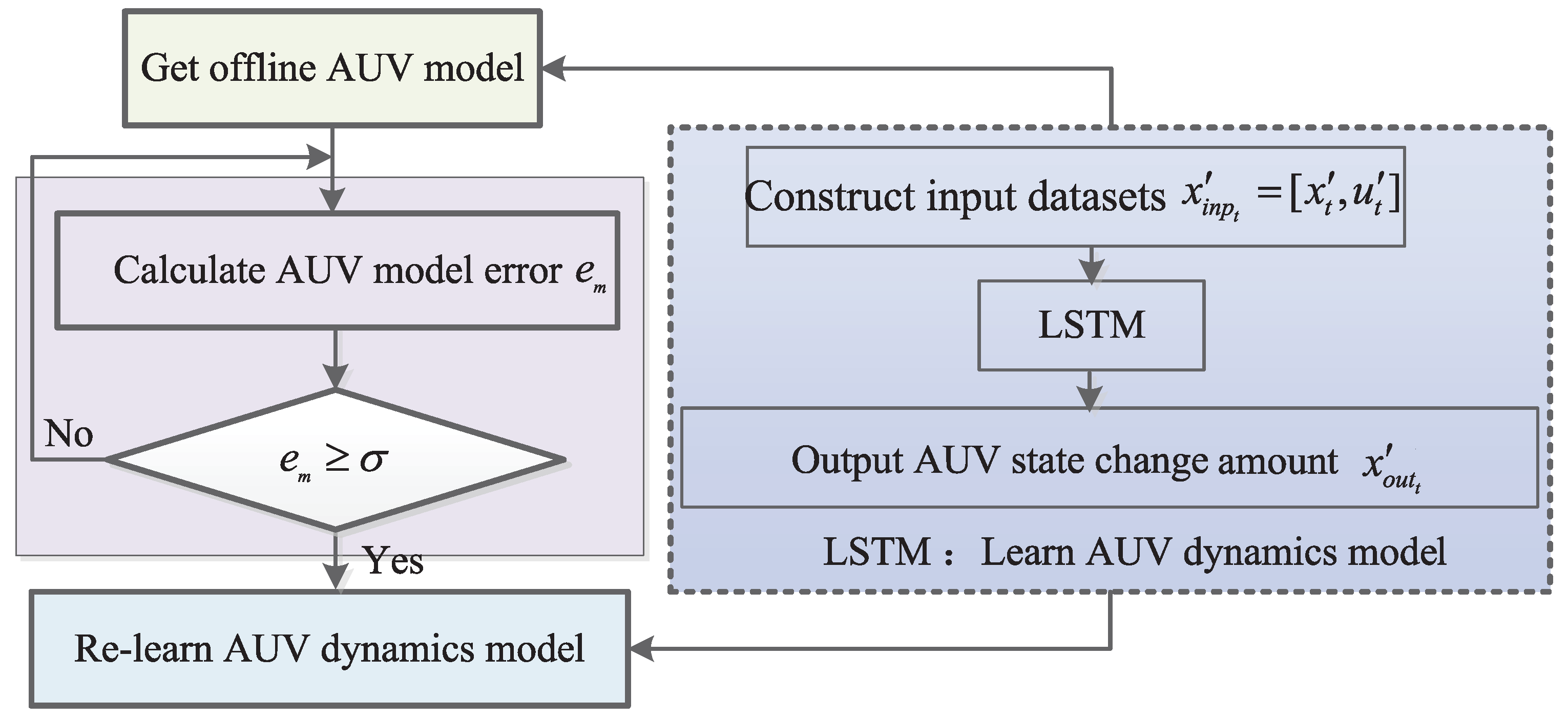
Figure 6 shows a detailed system model identification block diagram. Offline models can be obtained by offline training through real historical data. During the actual sailing, the system will regularly check the accuracy of the learned dynamics model. If the error is greater than $\sigma$ pre-determined empirically and does not meet the requirements, the model will be retrained based on new real-time data.

4. Results

In order to verify the effectiveness of the proposed method, numerous experiments have been performed. The experiments were divided into two parts based on simulation data (see Section 4.1) and real data (see Section 4.2). Simulations were run on the model described in Section 2. The real data were acquired by the Sailfish AUV.

4.1. Results on Simulation Data

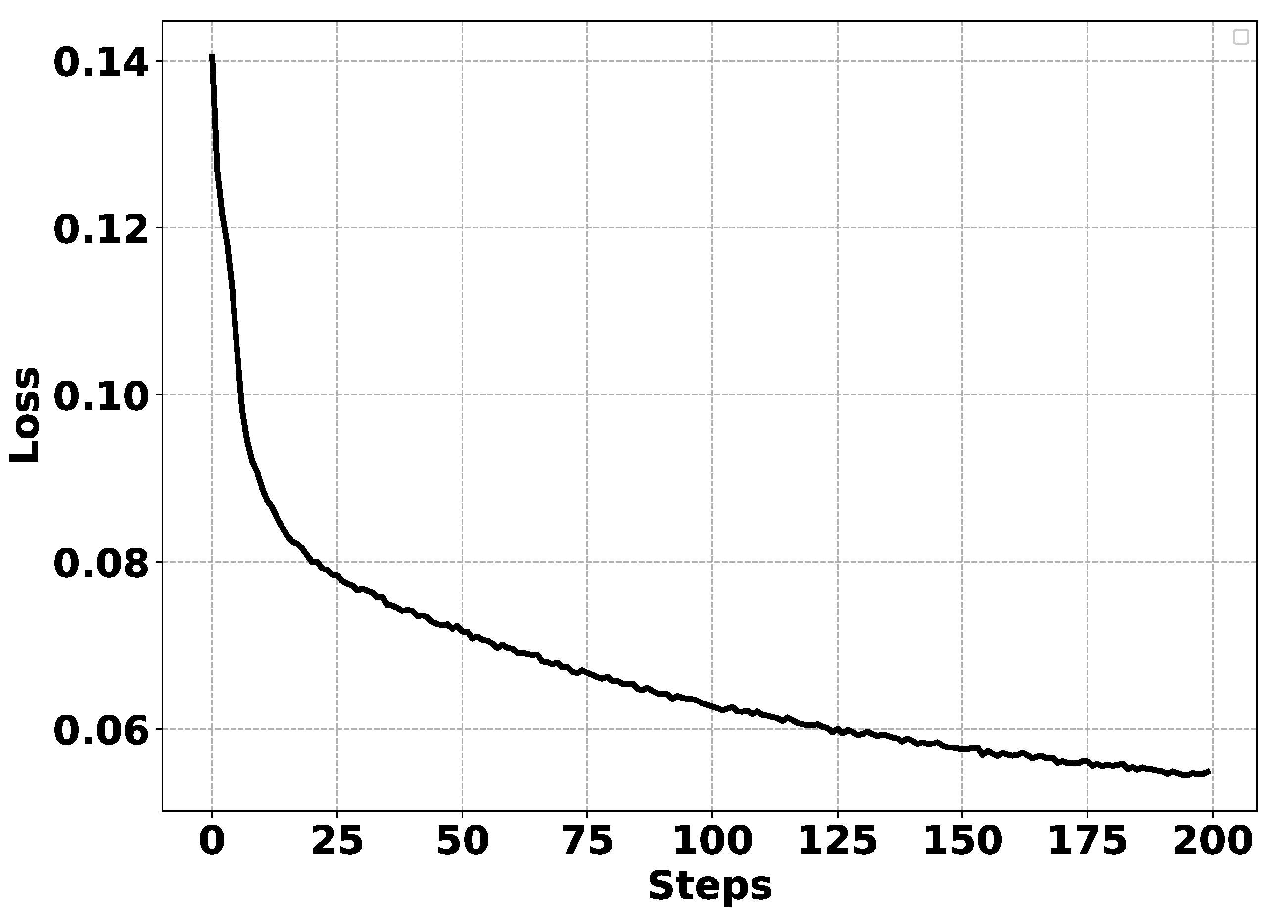
First, the validity of AUV system identification based on the LSTM neural network is verified. A set of hyperparameters is randomly set for the LSTM neural network, and a system identification experiment is carried out for the above AUV simulation system. In total, 4990 input and output data pairs are used for model identification, of which 4000 sets of data are used as training sets to train the LSTM neural network. The other 990 sets of data are used as validation sets to test the recognition effect of the model. The number of training is set to 100.

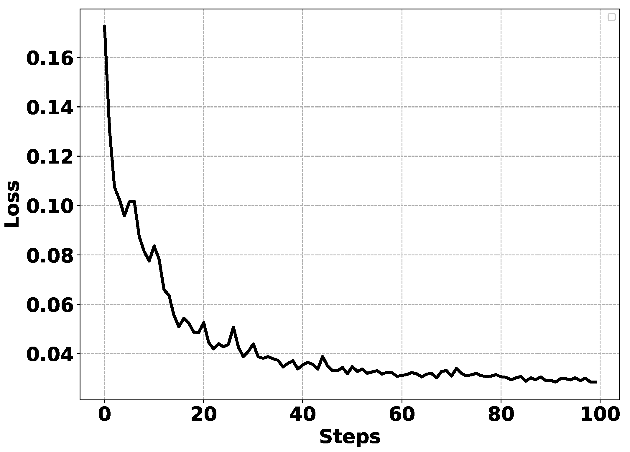
The change curve of the loss function during training is shown in Figure 7. As shown in the figure, the loss curve converges during training, and the value of the loss function decreases with iterations. From the perspective of the convergence of the loss curve, the application of the LSTM neural network can effectively realize the identification of the AUV system.

After 100 times of training, the validation dataset is brought into the network model to test. After calculation, the squared sum of the output error is 8.490711, and the mean and variance of the absolute value of the error are 0.1761263 and 0.0145471, respectively. We can see that the output of the LSTM network model can fit the actual output of the system after 100 times of training. However, the error between the network output and the real output is large. The fitting curve between the network output and the real output will be shown in the comparison results of different methods later.

The large output fitting error of the above LSTM neural network model is because the hyperparameter settings of the model are not suitable. The identification accuracy is greatly affected by the network hyperparameter settings. Inappropriate hyperparameter settings may even lead to non-convergence. In order to achieve high-precision system identification, a reinforcement learning algorithm is used to optimize the selection of the hyperparameters of the above neural network.

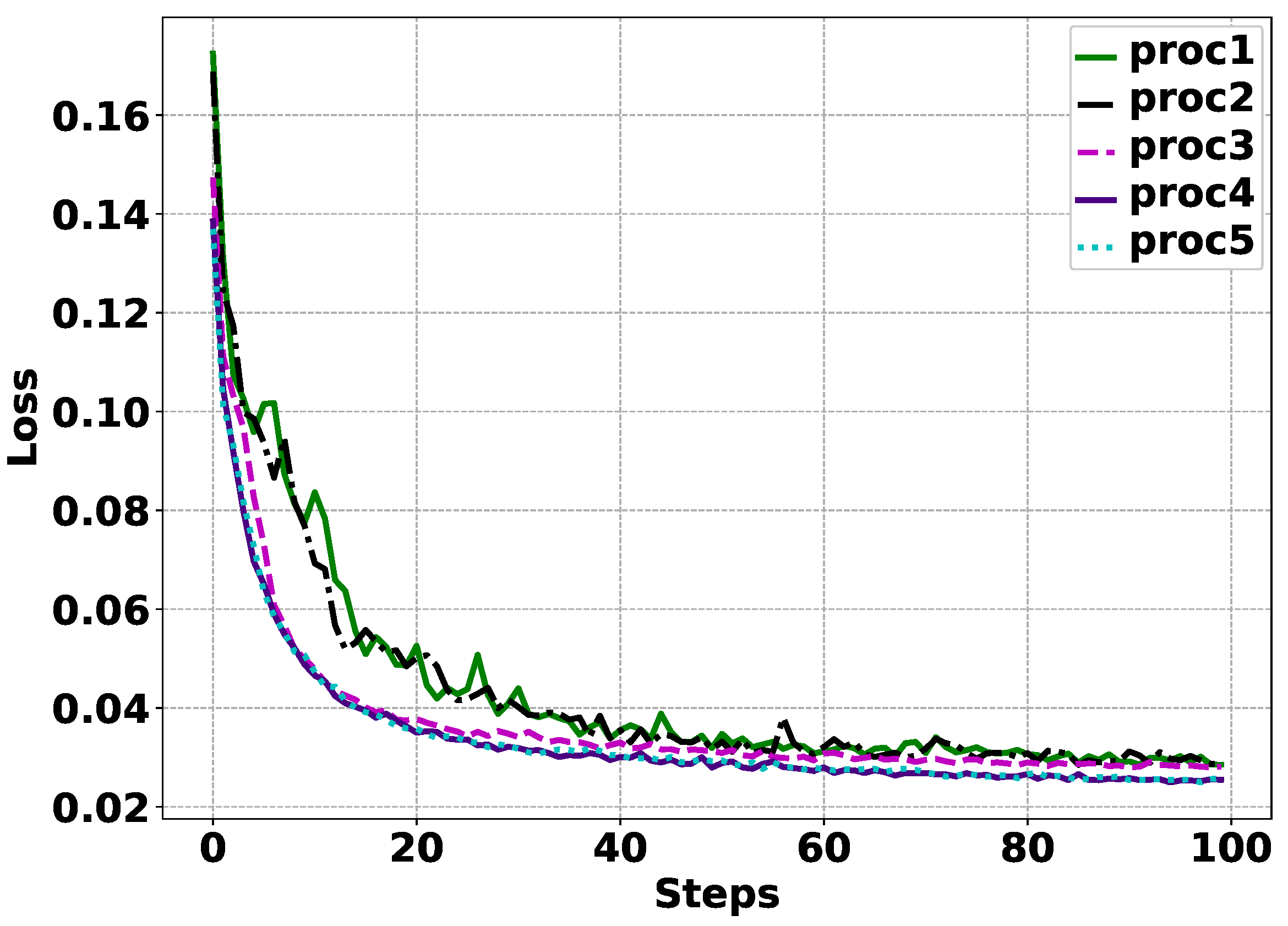
Data were divided into training and test sets during each test, yielding a training set of 4000 and a test set of 990. The proposed method was performed for 100 episodes. To demonstrate the optimization performance of the method, we compare the results of five different stages (proc1-0th episode, proc2-25th episode, proc3-50th episode, proc4-75th episode, and proc5-100th episode).

We can see from the above results that the five optimized LSTM neural network models can make the loss curve converge quickly, shown in Figure 8. It can be also noticed that the convergence speed increases as the episode increases, and this method has prominent optimization characteristics.

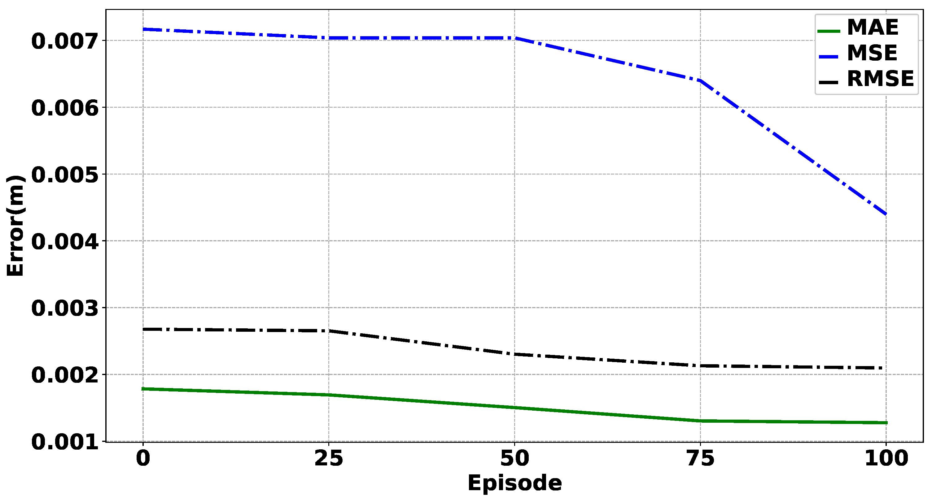
The statistical results of the output errors of the five groups of LSTM neural network models on the validation set are recorded in

Table 4. Results of LSTM neural network hyperparameter optimization.

Episode	Hyperparameter Combination	Mean Absolute Error	Mean Squared Error	Root Mean Square Error
0	$(50,50,8,10)$	$0.001784$	$7.167763\times {10}^{-6}$	$0.002677$
25	$(100,100,32,15)$	$0.001693$	$7.037789\times {10}^{-6}$	$0.002652$
50	$(100,150,8,20)$	$0.001503$	$6.737789\times {10}^{-6}$	$0.002302$
75	$(150,50,32,15)$	$0.001304$	$6.397751\times {10}^{-6}$	$0.002129$
100	$(50,100,8,10)$	$0.001277$	$4.396948\times {10}^{-6}$	$0.002096$

. In order to make the trend of MSE more apparent, it is enlarged 1000 times and displayed in Figure 9. As can be seen from the graph, the MAE, MSE and RMSE of the error of making predictions on the validation set decrease as the number of episodes increases. The above results also demonstrate the performance of the method from a statistical point of view.

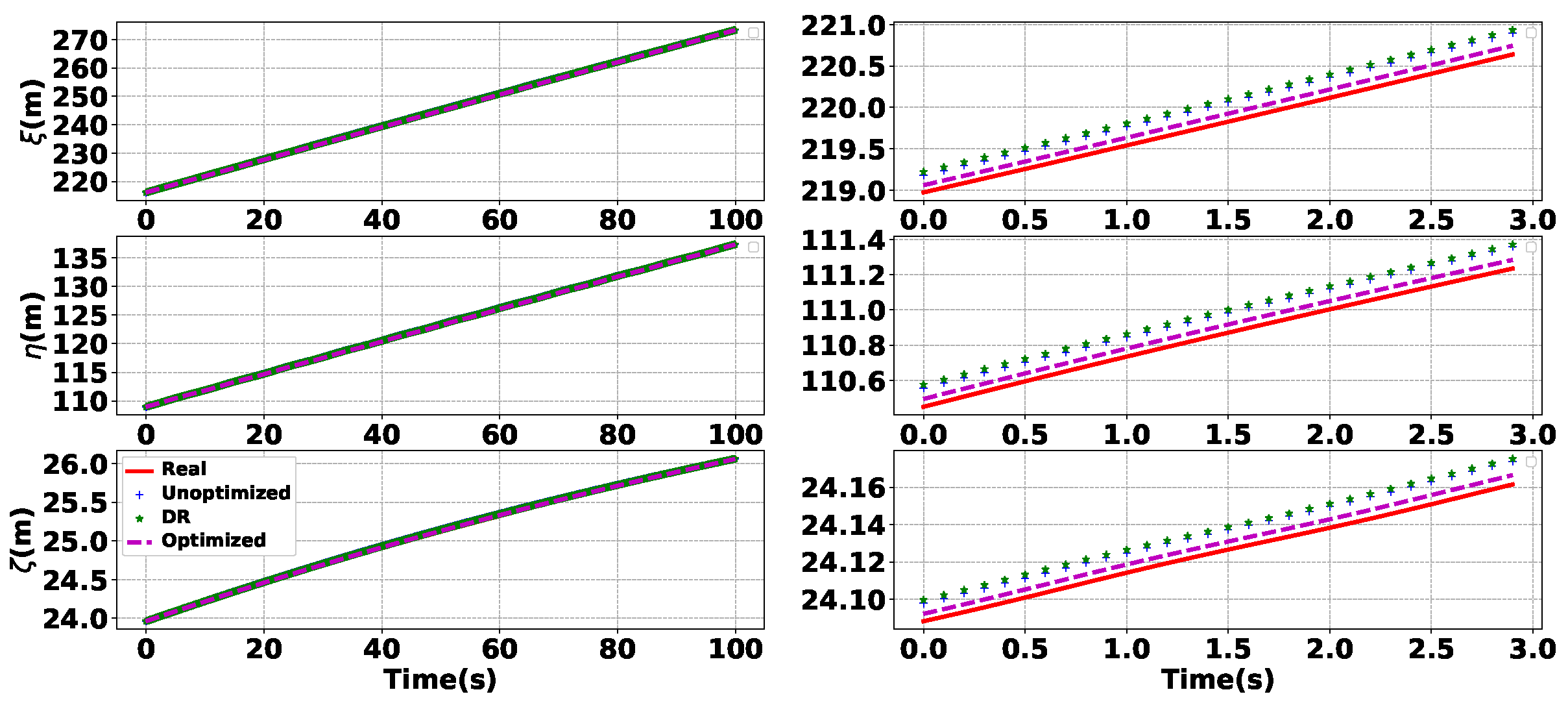
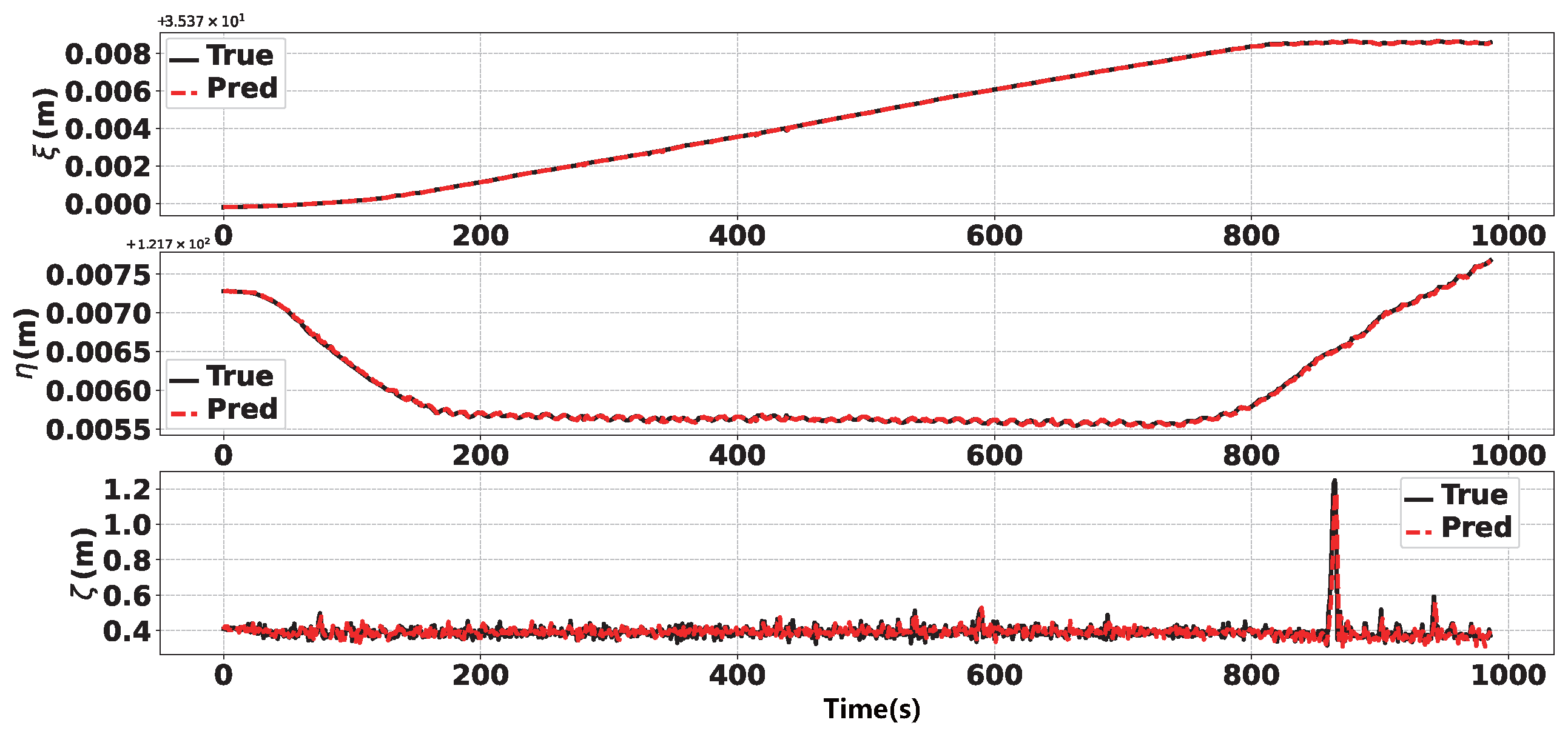
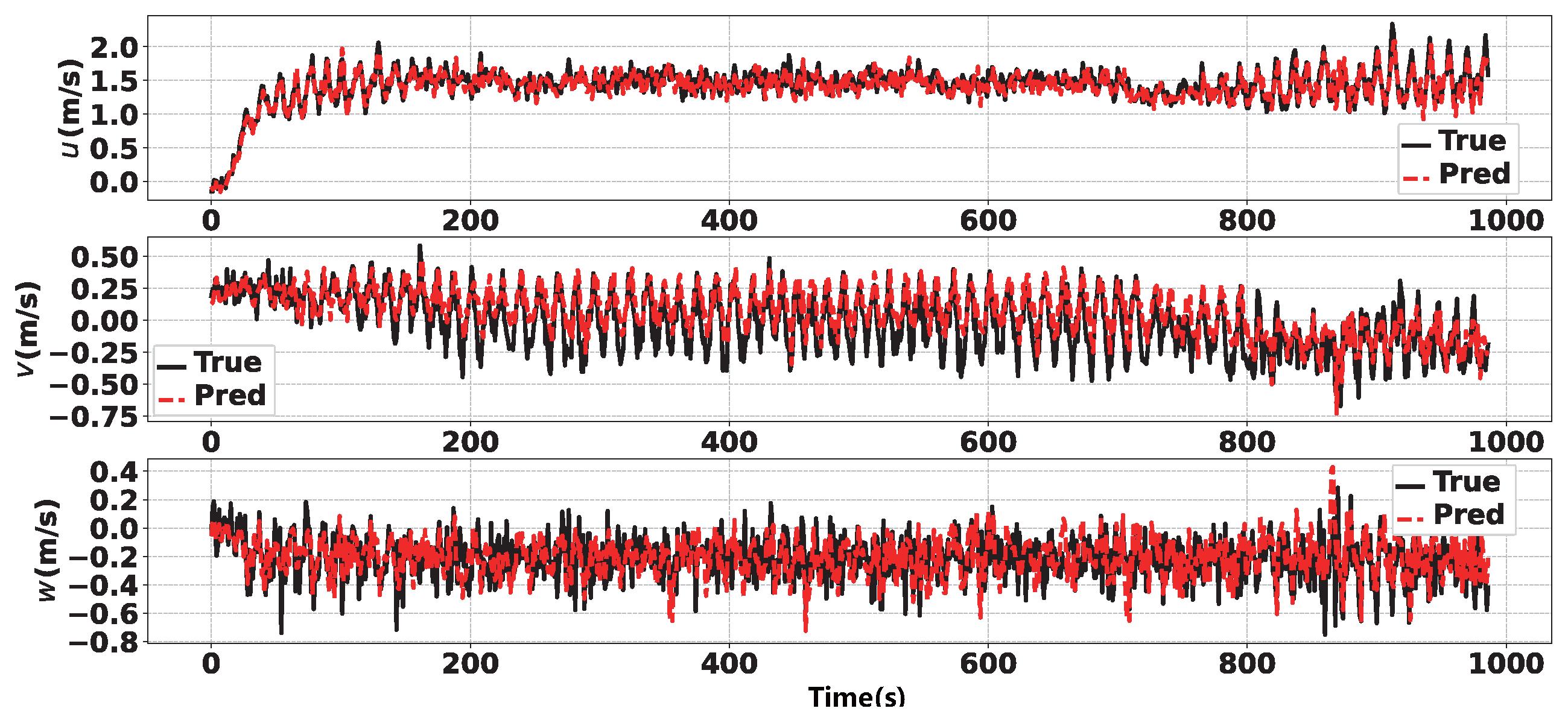
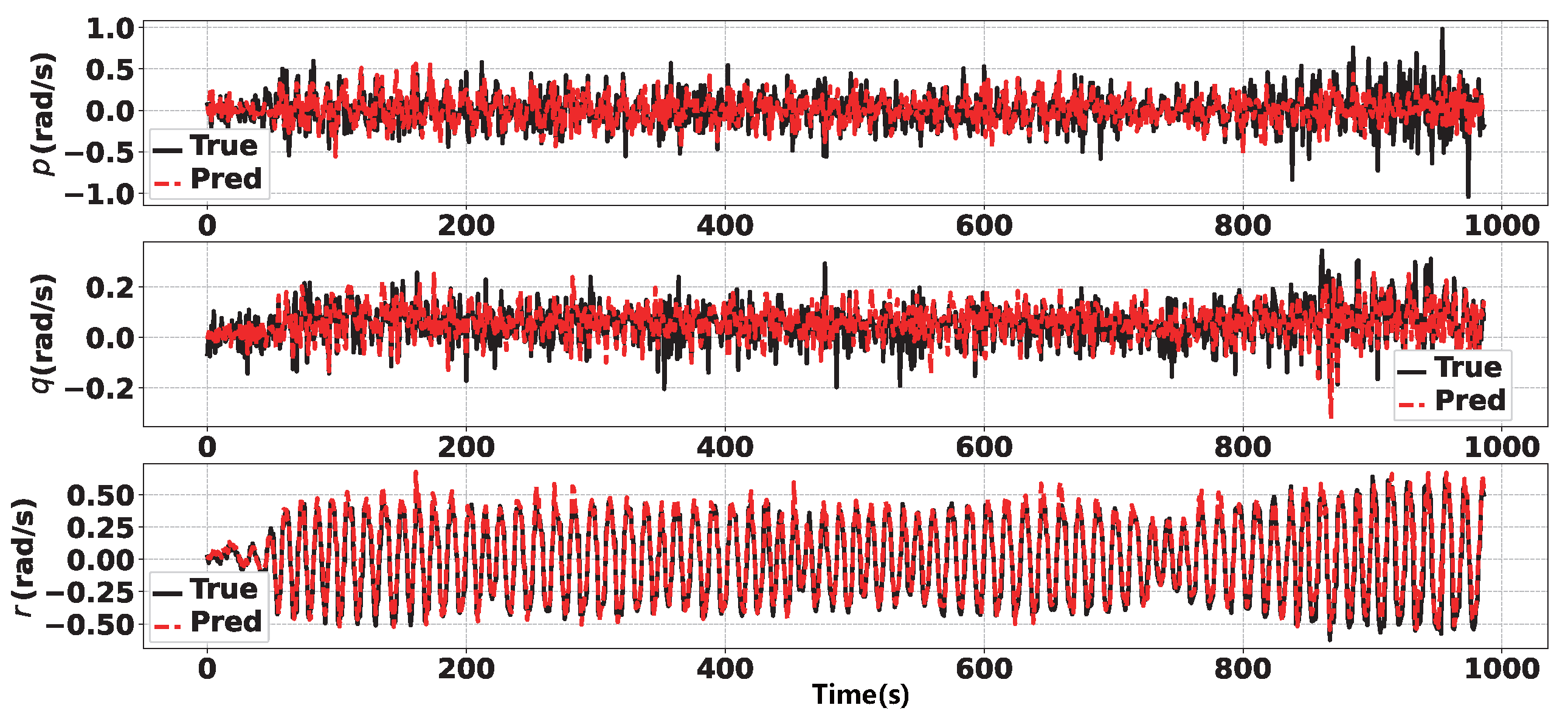
In order to further illustrate the advantages of this method, we compared the effect of the method before and after optimization with the commonly used DR algorithm. We compare the prediction results on the validation set optimized after 0 episodes and 100 episodes with the results predicted by the DR algorithm. The fitting curves of the network output and the real output of the AUV’s position, linear velocity, angle, and angular velocity are shown in Figure 10, Figure 11, Figure 12 and Figure 13, respectively. It can be seen from the figure that the optimized LSTM model makes the output of the 12 variables of the identification model have better agreement with the actual system output. In order to more clearly reflect the effectiveness of the method proposed in this paper, the MAE, MSE, and RMSE indicators of the prediction error are shown in

Table 5. Error comparison of different methods.

Method	MAE	MSE	RMSE
Unoptimized	$0.001784$	$7.167763\times {10}^{-6}$	$0.002677$
DR	$0.001802$	$7.203546\times {10}^{-6}$	$0.002825$
Optimized method	$0.001277$	$4.396948\times {10}^{-6}$	$0.002096$

. Compared with the unoptimized approach and DR, our method shows superior performance, with less MAE (28.42%, 29.13%), MSE (38.66%, 38.96%), and RMSE (21.70%, 25.81%). It can be seen that the deviation between the output of our method and the actual system is smaller than that of the other two methods.

4.2. Results on Real Data

The AUV dataset is required for training and validating the LSTM neural network model identification method. Therefore, the experiments of data collection should be carried out first. The experiments were carried out on the Sailfish AUV, as shown in Figure 14.

The actual data includes the sensor’s noise in the acquisition process, and it is more difficult to obtain an accurate model than the simulation. Therefore, the method performed 200 episodes. The experimental dataset is divided into training and testing sets, yielding a training set of 4000 and a test set of 990. From the loss curve of the LSTM neural network in the training process, this method has prominent learning characteristics, as shown in Figure 15.

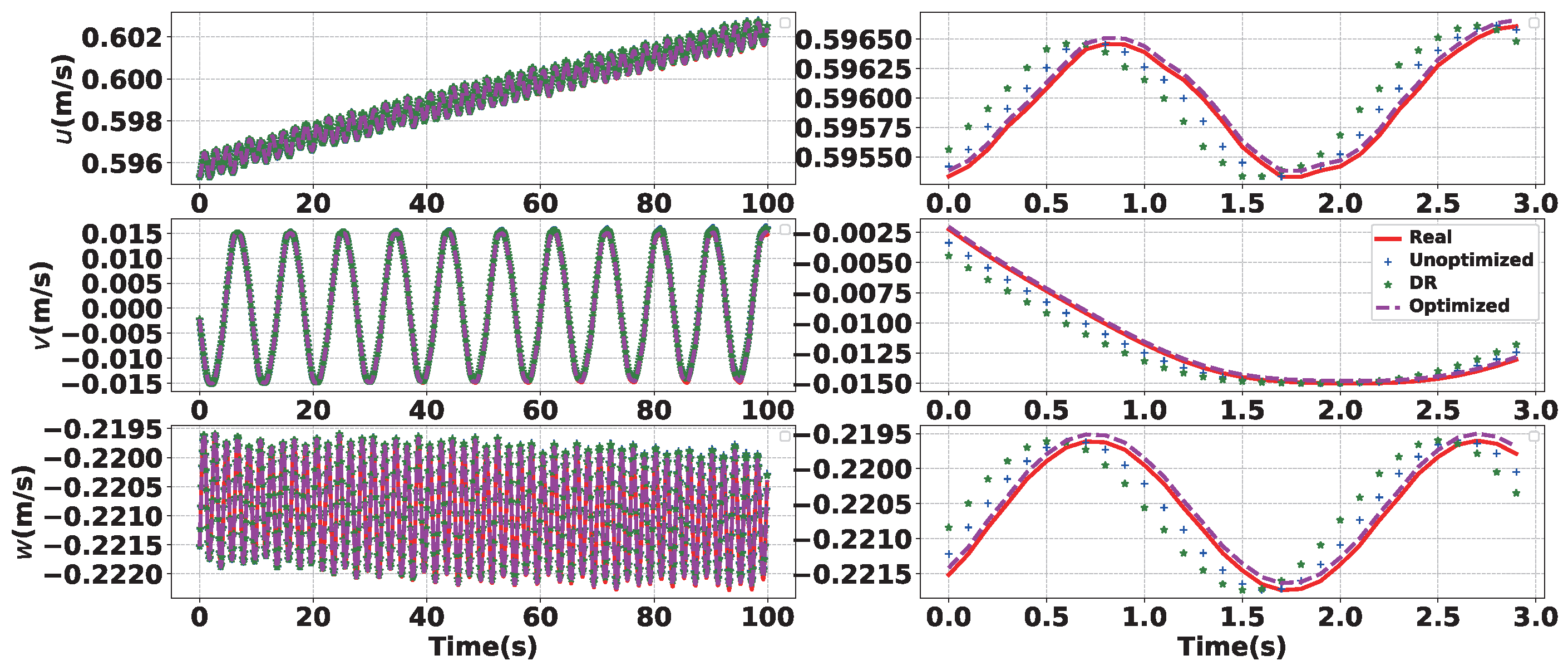
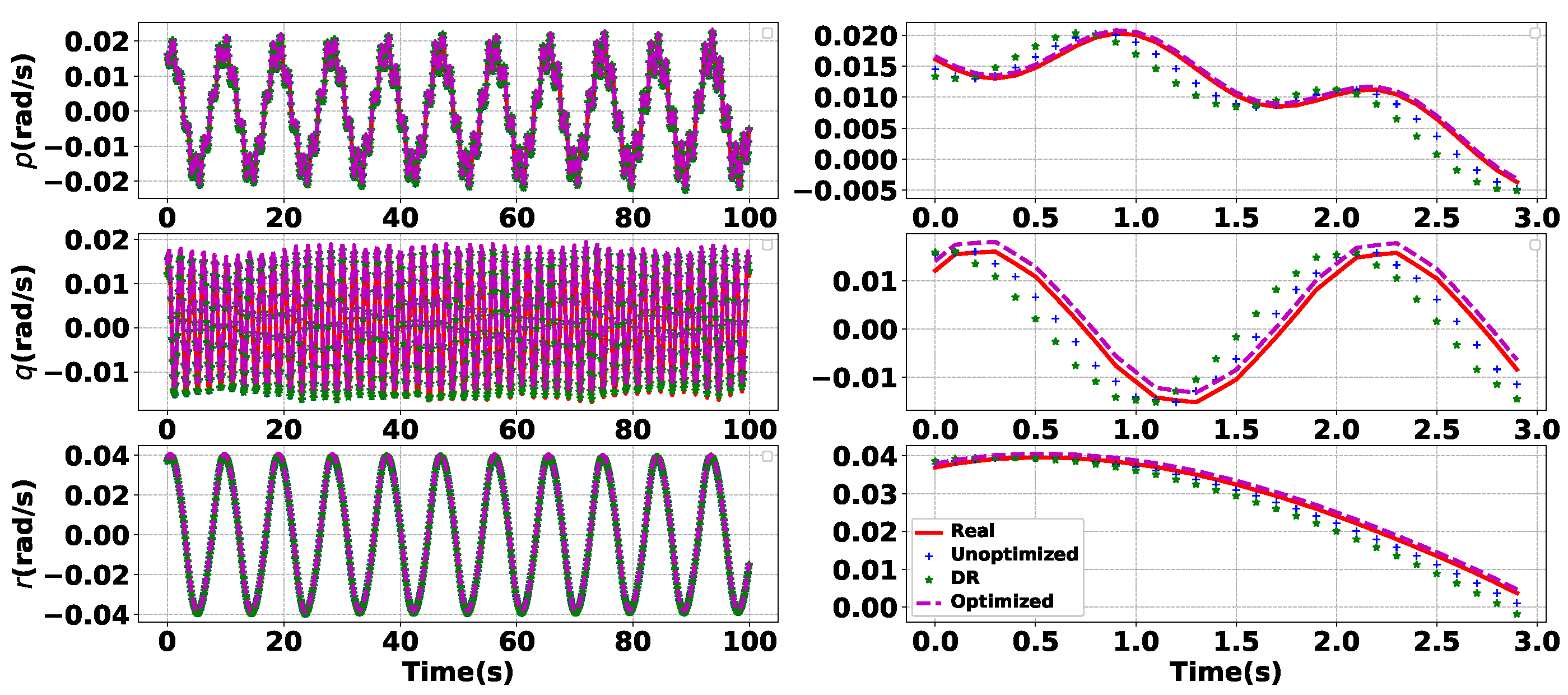
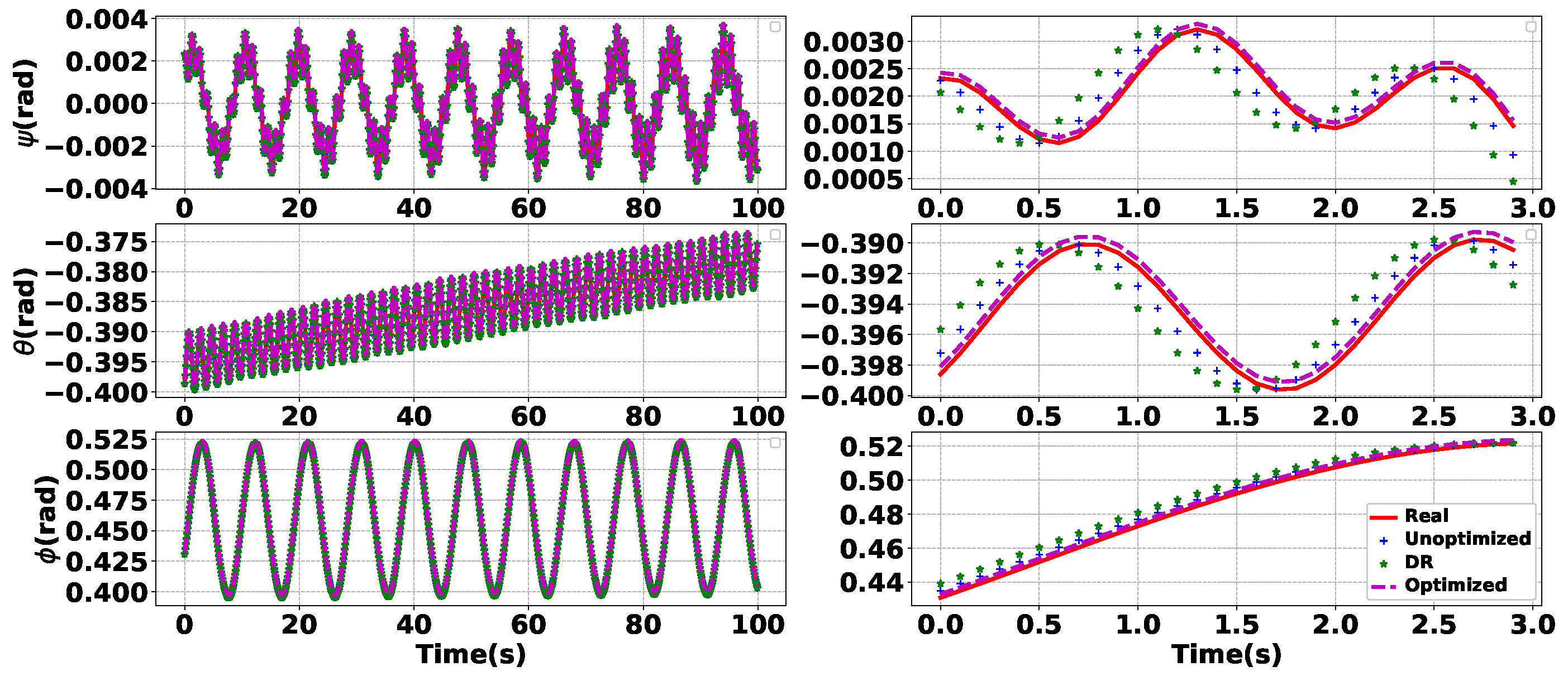
The fitting curve between the network output and the real output is shown in Figure 16, Figure 17, Figure 18 and Figure 19. The calculated MSE of the output error is 550.830181, and the MAE and RMSE values are 6.250734 and 23.469771, respectively. We can see that the LSTM neural network obtained by optimization can fit the system’s actual output and achieve high-precision recognition of AUVs. In order to illustrate the superiority of the method, it is compared with the commonly used dead reckoning (DR) method. The results are shown in

Table 6. Error comparison of different methods.

Method	MAE	MSE	RMSE
Proposed method	$6.250734$	$206.830181$	$23.469771$
DR	$17.808035$	$550.071027$	$37.705304$

, the proposed method provided 64.90% higher MAE, 64.20% higher MSE, and 37.76% higher RMSE than the DR method.

Due to the small prediction bias for the AUV motion state, It turns out, yet again, that the proposed method has high predictive power. Therefore, the proposed identification method is of great significance to the actual navigation control of AUV.

5. Conclusions

Aiming at the identification problem of the AUV system, this paper adopts a neural network hyperparameter optimization method based on Q-Learning. This method has been experimentally verified, and the conclusions can be summarized as follows:

1. The LSTM framework has the characteristics of natural Markovization, which can model time series data with high precision. It is found that the historical data of AUV implies the causal relationship of its dynamic model and has the characteristics of a hidden Markov model. The experimental results also show that the adopted method can predict the AUV model well.

2. Optimally selecting hyperparameters can significantly improve the efficiency of LSTMs in specific tasks. It is concluded that the improved Q-learning method can make the LSTM neural network realize the high-precision identification of the AUV system.

3. The offline training in the system model identification framework can reduce online learning time and ensure the security of the initial online use. The online learning model can also ensure its validity.

4. The proposed method has high model identification accuracy and has certain application prospects. We can apply this method to fault diagnosis of AUV, design of the model-based controller, and other aspects.

However, the hyperparameter optimization method only considers recognition accuracy. Our method can potentially be improved in the convergence speed. Moreover, the performance of the LSTM and the improved Q method used in this paper still has certain limitations. We will improve the identification method and optimization method later.

References

- Fang, Y.; Huang, Z.; Pu, J.; Zhang, J. AUV position tracking and trajectory control based on fast-deployed deep reinforcement learning method. Ocean Eng. 2022, 245, 110452. [Google Scholar] [CrossRef]
- Praczyk, T. Using Neuro—Evolutionary Techniques to Tune Odometric Navigational System of Small Biomimetic Autonomous Underwater Vehicle—Preliminary Report. J. Intell. Robot. Syst. 2020, 100, 363–376. [Google Scholar] [CrossRef] [Green Version]
- Yuan, C.; Licht, S.; He, H. Formation Learning Control of Multiple Autonomous Underwater Vehicles With Heterogeneous Nonlinear Uncertain Dynamics. IEEE Trans. Cybern. 2018, 48, 2920–2934. [Google Scholar] [CrossRef] [PubMed]
- Qiao, L.; Zhang, W. Adaptive Second-Order Fast Nonsingular Terminal Sliding Mode Tracking Control for Fully Actuated Autonomous Underwater Vehicles. IEEE J. Ocean. Eng. 2019, 44, 363–385. [Google Scholar] [CrossRef]
- Min, F.; Pan, G.; Xu, X. Modeling of Autonomous Underwater Vehicles with Multi-Propellers Based on Maximum Likelihood Method. J. Mar. Sci. Eng. 2020, 8, 407. [Google Scholar] [CrossRef]
- Deng, F.; Levi, C.; Yin, H.; Duan, M. Identification of an Autonomous Underwater Vehicle hydrodynamic model using three Kalman filters. Ocean Eng. 2021, 229, 108962. [Google Scholar] [CrossRef]
- Wu, B.; Han, X.; Hui, N. System Identification and Controller Design of a Novel Autonomous Underwater Vehicle. Machines 2021, 9, 109. [Google Scholar] [CrossRef]
- Wang, D.; He, B.; Shen, Y.; Li, G.; Chen, G. A Modified ALOS Method of Path Tracking for AUVs with Reinforcement Learning Accelerated by Dynamic Data-Driven AUV Model. J. Intell. Robot. Syst. 2022, 104, 1–23. [Google Scholar] [CrossRef]
- Bresciani, M.; Costanzi, R.; Manzari, V.; Peralta, G.; Terracciano, D.S.; Caiti, A. Dynamic parameters identification for a longitudinal model of an AUV exploiting experimental data. In Proceedings of the Global Oceans 2020: Singapore—U.S. Gulf Coast, Biloxi, MS, USA, 5–30 October 2020; pp. 1–6. [Google Scholar]
- Jiang, C.m.; Wan, L.; Sun, Y.S. Design of motion control system of pipeline detection AUV. J. Cent. South Univ. 2017, 24, 637–646. [Google Scholar] [CrossRef]
- Wang, J.G.; Jiang, C.M.; Sun, Y.S.; He, B.; Li, J.Q. Neural network identification of underwater vehicle by hybrid learning algorithm. Zhongnan Daxue Xuebao (Ziran Kexue Ban)/J. Cent. South Univ. (Sci. Technol.) 2011, 42, 427–431. [Google Scholar]
- Muñoz Palacios, F.; Cervantes Rojas, J.S.; Valdovinos, J.; Sandre Hernandez, O.; Salazar, S.; Romero, H. Dynamic Neural Network-Based Adaptive Tracking Control for an Autonomous Underwater Vehicle Subject to Modeling and Parametric Uncertainties. Appl. Sci. 2021, 11, 2797. [Google Scholar] [CrossRef]
- Kim, D.; Park, M.; Park, Y.L. Probabilistic Modeling and Bayesian Filtering for Improved State Estimation for Soft Robots. IEEE Trans. Robot. 2021, 37, 1728–1741. [Google Scholar] [CrossRef]
- Zhang, T.; Zheng, X.Q.; Liu, M.X. Multiscale attention-based LSTM for ship motion prediction. Ocean Eng. 2021, 230, 109066. [Google Scholar] [CrossRef]
- Shahi, T.B.; Shrestha, A.; Neupane, A.; Guo, W. Stock Price Forecasting with Deep Learning: A Comparative Study. Mathematics 2020, 8, 1441. [Google Scholar] [CrossRef]
- Yam, L.; Yan, Y.; Jiang, J. Vibration-based damage detection for composite structures using wavelet transform and neural network identification. Compos. Struct. 2003, 60, 403–412. [Google Scholar] [CrossRef]
- Dahunsi, O.; Pedro, J. Neural Network-Based Identification and Approximate Predictive Control of a Servo-Hydraulic Vehicle Suspension System. Eng. Lett. 2010, 18, 357. [Google Scholar]
- Liu, J.; Du, J. Composite learning tracking control for underactuated autonomous underwater vehicle with unknown dynamics and disturbances in three-dimension space. Appl. Ocean Res. 2021, 112, 102686. [Google Scholar] [CrossRef]
- Dong, X.; Shen, J.; Wang, W.; Shao, L.; Ling, H.; Porikli, F. Dynamical Hyperparameter Optimization via Deep Reinforcement Learning in Tracking. IEEE Trans. Pattern Anal. Mach. Intell. 2019, 43, 1515–1529. [Google Scholar] [CrossRef]
- Mercangöz, M.; Cortinovis, A.; Schönborn, S. Autonomous Process Model Identification using Recurrent Neural Networks and Hyperparameter Optimization. IFAC-PapersOnLine 2020, 53, 11614–11619. [Google Scholar] [CrossRef]
- Sena, M.; Erkilinc, M.S.; Dippon, T.; Shariati, B.; Emmerich, R.; Fischer, J.K.; Freund, R. Bayesian Optimization for Nonlinear System Identification and Pre-Distortion in Cognitive Transmitters. J. Light. Technol. 2021, 39, 5008–5020. [Google Scholar] [CrossRef]
- Baker, B.; Gupta, O.; Naik, N.; Raskar, R. Designing Neural Network Architectures using Reinforcement Learning. arXiv 2016, arXiv:1611.02167. [Google Scholar]
- Chen, S.; Wu, J.; Liu, X. EMORL: Effective multi-objective reinforcement learning method for hyperparameter optimization. Eng. Appl. Artif. Intell. 2021, 104, 104315. [Google Scholar] [CrossRef]
- Liu, X.; Wu, J.; Chen, S. A context-based meta-reinforcement learning approach to efficient hyperparameter optimization. Neurocomputing 2022, 478, 89–103. [Google Scholar] [CrossRef]
- Mnih, V.; Kavukcuoglu, K.; Silver, D.; Graves, A.; Antonoglou, I.; Wierstra, D.; Riedmiller, M.A. Playing Atari with Deep Reinforcement Learning. arXiv 2013, arXiv:1312.5602. [Google Scholar]
- Schulman, J.; Wolski, F.; Dhariwal, P.; Radford, A.; Klimov, O. Proximal Policy Optimization Algorithms. arXiv 2017, arXiv:1707.06347. [Google Scholar]
- Watkins, C.; Dayan, P. Technical Note: Q-Learning. Mach. Learn. 1992, 8, 279–292. [Google Scholar] [CrossRef]
- Nouri, N.M.; Valadi, M.; Asgharian, J. Optimal input design for hydrodynamic derivatives estimation of nonlinear dynamic model of AUV. Nonlinear Dyn. 2018, 92, 139–151. [Google Scholar] [CrossRef]
- Prestero, T. Verification of a Six-Degree of Freedom Simulation Model for the REMUS Autonomous Underwater Vehicle. Ph.D. Thesis, Massachusetts Institute of Technology, Cambridge, MA, USA, 2011. [Google Scholar]
- Rashid, T.; Hassan, M.; Mohammadi, M.; Fraser, K. Improvement of Variant Adaptable LSTM Trained With Metaheuristic Algorithms for Healthcare Analysis. In Research Anthology on Artificial Intelligence Applications in Security; Information Resources Management Association: Hershey, PA, USA, 2021; pp. 1031–1051. [Google Scholar]
- Rashid, T.A.; Fattah, P.; Awla, D.K. Using Accuracy Measure for Improving the Training of LSTM with Metaheuristic Algorithms. Procedia Comput. Sci. 2018, 140, 324–333. [Google Scholar] [CrossRef]
- Hochreiter, S.; Schmidhuber, J. Long Short-Term Memory. Neural Comput. 1997, 9, 1735–1780. [Google Scholar] [CrossRef]
- Sutton, R.; Barto, A. Reinforcement Learning: An Introduction. IEEE Trans. Neural Netw. 1998, 9, 1054. [Google Scholar] [CrossRef]
Figure 1.
AUV body-fixed and earth-fixed coordinate systems.
Figure 2.
The structure of the LSTM neural network.
Figure 3.
One-step AUV dynamic model based on LSTM.
Figure 4.
The basic structure of reinforcement learning.
Figure 5.
The Structure of hyperparameter optimization method based on Q-Learning.
Figure 6.
Block diagram of AUV model identification.
Figure 7.
The result of loss before optimization.
Figure 8.
Loss results at different stages.
Figure 9.
Error results at different stages.
Figure 10.
Identification result of AUV position.
Figure 11.
Identification result of AUV velocity.
Figure 12.
Identification result of AUV angular velocity.
Figure 13.
Identification result of AUV attitude angle.
Figure 14.
Sailfish AUV platform during the experiment.
Figure 15.
The training loss curve of the proposed LSTM neural network.
Figure 16.
Figure 17.
Figure 18.
Figure 19.