Uncertainties in Liner Shipping and Ship Schedule Recovery: A State-of-the-Art Review

Abstract

Each shipping line is expected to establish a reliable operating model, and the design of ship schedules is a key operational consideration. Long-term profits for shipping lines can be expected from a well-designed ship schedule. In today’s liner service design, managing the time factor is critical. Shipping schedules are prone to different unexpected disruptions. Such disruptions would necessitate a near-real-time analysis of port capacity and re-design of the original ship schedule to offset the negative externalities. Ship schedule recovery strategies should be implemented to mitigate the effects caused by disruptions at ports or at sea, which may include, but are not limited to, ship sailing speed adjustment, handling rate adjustment at ports, port skipping, and port skipping with container diversion. A proper selection of ship schedule recovery strategies is expected to minimize deviations from the original ship schedule and reduce delays in the delivery of cargoes to the destination ports. This article offers a thorough review of the current liner shipping research primarily focusing on two major themes: (1) uncertainties in liner shipping operations; and (2) ship schedule recovery in response to disruptive events. On the basis of a detailed review of the available literature, the obtained results are carefully investigated, and limitations in the current state-of-the-art are determined for every group of studies. Furthermore, representative mathematical models are provided that could be further used in future research efforts dealing with uncertainties in liner shipping and ship schedule recovery. Last but not least, a few prospective research avenues are suggested for further investigation.

1. Introduction

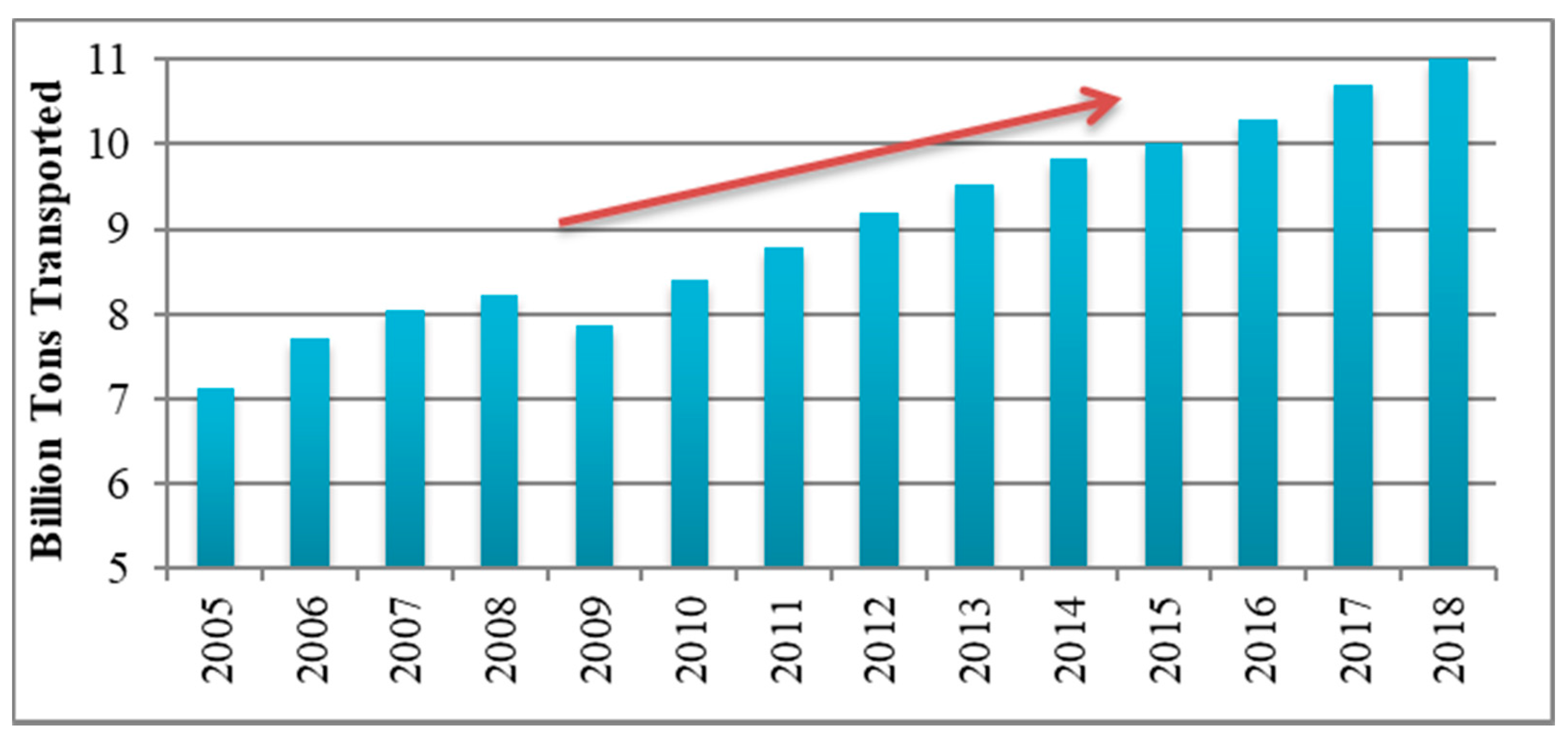
1.1. Background

Maritime transport outperforms other transportation modes in terms of the amount of transported cargoes measured in ton-kilometers. The proportion of cargo moved by sea varies from year to year, but in the recent years, waterborne trade in the United States (USA) has represented between 22 and 24 percent of the total ton-kilometer cargo movements, which is more than $1.5 trillion worth of goods [1]. Overall, this results in a yearly economic output of $5.4 trillion. The maritime transportation system plays an important role in Europe as well. According to the European Commission, waterborne trade between nations (also known as short-sea shipping) accounts for nearly 41 percent of the freight transport market in Europe [1]. Due to the lower cost of maritime transport in comparison to other modes of shipping, such as air freight, international seaborne trade has increased by 67 percent in terms of weight between 1980 and 2007 [2]. Moreover, the international waterborne trade volumes have been constantly growing since 2009 and reached approximately 11.0 billion tons in 2018, which is more than a 40% increase compared to 2009 (see Figure 1). Nevertheless, in comparison to other modes of transportation, the sea freight industry is facing unprecedented and chaotic conditions, such as port congestion, labor strikes, severe weather conditions, shipping container shortages, and customs delays [3,4,5,6]. After the analysis of 5410 ship arrivals at ports, Drewry Shipping determined that approximately 21% of ships were one day behind the planned arrival, whereas 22% of ships were delayed by two or more days [7].

Weather can have a critical impact on ships carrying cargo. Given that transport is an inherently logistical industry relying on the surrounding physical infrastructure, it is constantly exposed to the whims of the natural environment. While most cargo ships can withstand extreme inclement weather conditions, strong tropical cyclones (e.g., hurricanes, typhoons) can make sailing and port operations too dangerous. Adverse weather conditions may cause significant delays in ship arrivals at ports and result in substantial monetary losses. As an example, about USD 12 billion worth of damage was incurred to the Japanese maritime infrastructure during the 2011 Tohoku tsunami on Japan’s Pacific Coast [8]. The Ports of Felixstowe and Southampton, which are considered some of the largest container ports in the United Kingdom, experienced severe ship service disruptions as a result of strong winds in January 2012 [9]. The Port of New York/New Jersey was shut down for one week in November 2012 due to Hurricane Sandy. The 2019 North Atlantic hurricane season recorded a total of 18 named storms, 6 hurricanes, and 3 major hurricanes [10]. As a result of extreme weather events, the reliability of transpacific and transatlantic schedules fell below 40% in 2019. Furthermore, the container terminals in Baton Rouge (LA, USA) were completely shut down due to severe tropical storms in August 2020 [8].

As underlined by Notteboom [11], significant delays in liner shipping operations could be endured due to maritime passage, port access, and marine terminal operations. Channels play an important role in liner shipping operations, as they enable the passage of ships to the designated locations. However, many channels impose limitations on the ship size and may incur additional waiting time (especially, if certain ships do not follow the previously negotiated arrival time). Certain ports around the world are subject to the tidal effect, when the depth of access channels fluctuates throughout the day [12,13]. Oversized ships have to wait during particular time periods to ensure that the depth of the access channel will be safe to navigate. Safe ship navigation is critical, as navigational issues may disrupt channel operations and cause substantial delays (e.g., the 6-day Suez Canal obstruction caused by the large 20000-TEU ship “Ever Given” in 2021).

Considering increasing trade volumes and the existing terminal capacity constraints, the berth availability and handling equipment may not be always guaranteed, especially when the previously negotiated arrival time windows have been missed by the approaching ships. Ships that arrive outside the agreed time windows significantly disrupt marine terminal operations and cause port congestion. Labor strikes could be another reason for delays in container handling at marine terminals or even complete terminal shutdowns. As an example, a total of ten marine container terminals were shut down at the Ports of Los Angeles and Long Beach (USA) in November 2012 due to labor strikes [9]. The container traffic at both ports experienced a standstill. Equipment failures at marine container terminals are considered a rare event, but they do occur from time to time. The quay crane failure at the DP World Port Botany terminal (Sydney, Australia) caused a sudden disruption and unexpected slot cancellations in September 2013 [9].

The outbreak of COVID-19 is recognized as a major disruptive event for liner shipping and maritime transportation [14,15,16,17]. As a result of the global economic crisis that was caused by the COVID-19 pandemic, the international maritime trade volumes reduced by 4.1% in 2020 [14]. Marine terminal operators experienced significant challenges imposed by the pandemic. In particular, certain terminal operators had to shut down their terminals and quarantine their employees due to the fact that some of the employees tested positive for the virus [17]. The closure of marine terminals caused substantial supply chain disruptions. The ships loaded with import goods were queued in the vicinity of marine terminals but could not be served due to the terminal closures. Ship operations were subjected to national and municipal restrictions, which frequently resulted in port clearance delays [18]. Additional restrictions were imposed for the personnel embarking and disembarking, cargo loading and discharge, and ship refueling. Tensions in international trade resulted in trade pattern shifts and a search for alternative markets (e.g., a decrease in trade flows from China and a transition to other markets—[14]). The USA increased the exports of its merchandise to other countries, which assisted with the compensation for the decrease in exports from China.

1.2. Existing Research Gaps and Contributions of This Study

A large number of the existing research efforts were dedicated to the planning of different liner shipping operations, including fleet deployment [19,20,21,22,23], port service frequency determination [24,25,26,27], ship sailing speed optimization [28,29,30,31], and ship schedule design [32,33,34,35,36,37,38,39,40,41]. However, the existing research efforts generally do not account for potential uncertainties in liner shipping operations and do not model any recovery options that could be used to effectively respond to disruptions. Furthermore, a number of survey studies were conducted in the past aiming to provide a holistic overview of the liner shipping literature [42,43,44,45,46,47,48]. Nevertheless, there is still a lack of systematic literature surveys that specifically concentrate on uncertainties in liner shipping operations and ship schedule recovery. Considering the increase in the occurrence of disruptive events and their negative impacts on liner shipping operations, the present study aims to offer the following contributions to the state-of-the-art:

✓

A comprehensive up-to-date review of the liner shipping literature is conducted with a specific emphasis on uncertainties in liner shipping operations and ship schedule recovery.

✓

The collected studies are reviewed in a systematic way, capturing the main assumptions regarding sailing speed and port time modeling, objective(s) considered, key components of objective functions(s) considered, uncertain elements modeled, ship schedule recovery options modeled, solution approaches adopted, and certain specific considerations adopted.

✓

A representative mathematical formulation is presented for the ship scheduling problem with uncertainties, which can be used by shipping lines to assess the impacts of uncertainties on liner shipping operations and design robust ship schedules. Moreover, the proposed mathematical formulation can serve as a foundation for future efforts that concentrate on uncertainties in liner shipping operations.

✓

A set of representative mathematical formulations are presented for the ship schedule recovery problem with various recovery options (i.e., sailing speed adjustment, handling rate adjustment, port skipping, and port skipping with container diversion), which can be used by shipping lines to select the appropriate ship schedule recovery option(s). Furthermore, the proposed mathematical formulations can serve as a foundation for future efforts that concentrate on ship schedule recovery.

✓

Research gaps in previous and contemporary studies on uncertainties in liner shipping operations and ship schedule recovery are clearly identified, and future research areas that should be considered in the following years are specifically underlined.

The outcomes from this research are expected to assist the relevant stakeholders involved in liner shipping operations with improvements in the reliability of their schedules and selection of the appropriate recovery options in response to major disruptive events. Reliable ship schedules and appropriate recovery options will further decrease cargo delivery delays, improve customer service, and enhance the overall sustainability of maritime transport. The next sections of the manuscript contain the following information. Section 2 provides a detailed description of how the literature search was performed, aiming to capture the most relevant studies on uncertainties in liner shipping operations and ship schedule recovery. Section 3 presents a detailed description of the ship scheduling problem with uncertainties, a formulation of the supporting mathematical model, a review of the relevant studies, a literature summary, and future research needs in the area of uncertainties in liner shipping operations. After that, Section 4 presents a detailed description of the ship schedule recovery problem, formulations of the supporting mathematical models, a review of the relevant studies, a literature summary, and future research needs in the area of ship schedule recovery. The main study conclusions are provided in Section 5.

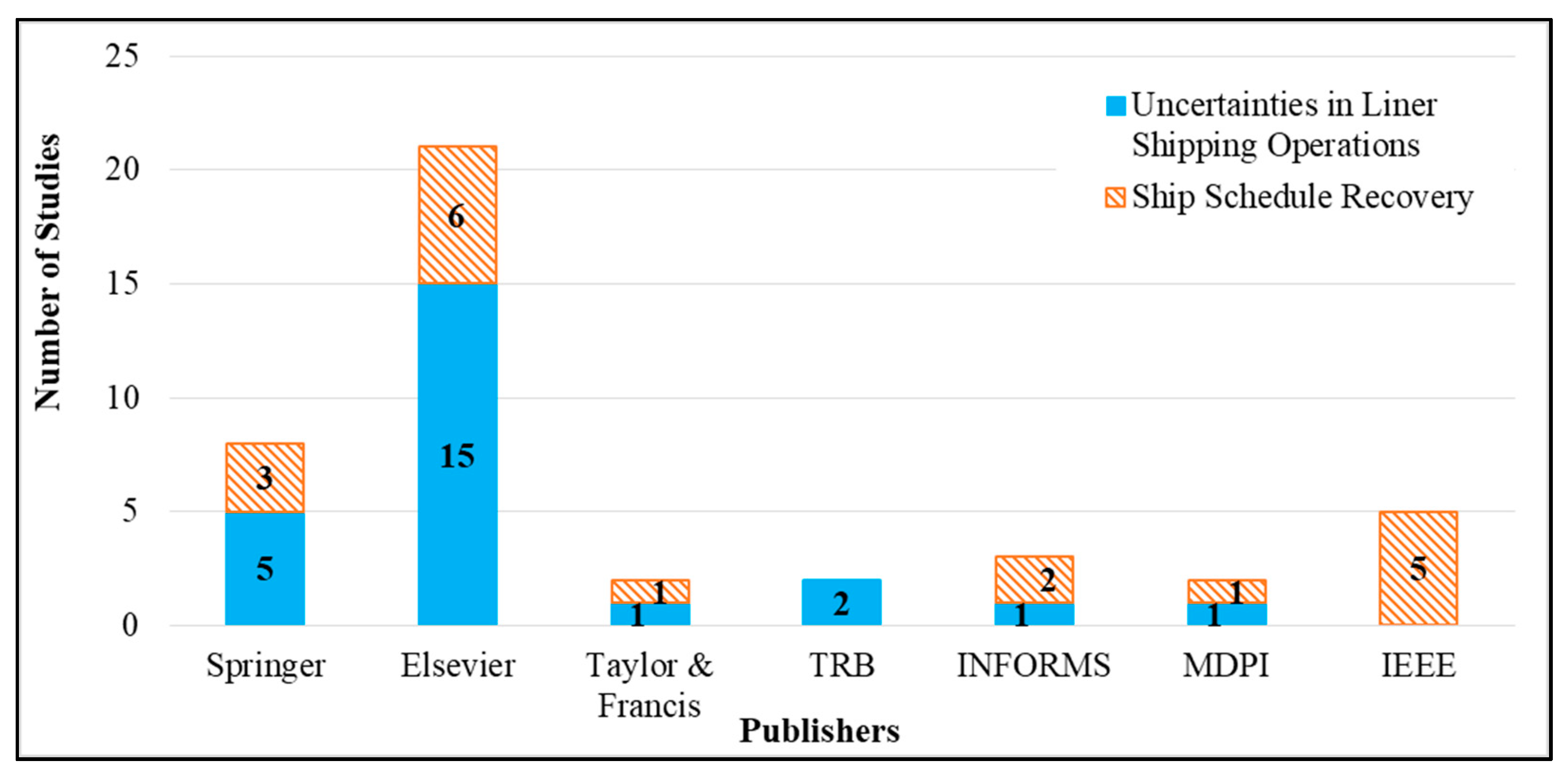
2. Literature Search

A thorough literature search is essential in order to perform a comprehensive survey study. As a part of this research effort, a detailed literature search was conducted by means of the content analysis method [49]. The following keywords and their combinations were used to guide the search process: “liner shipping”, “shipping lines”, “liner shipping companies”, “ship schedule design”, “vessel schedule design”, “ship timetable design”, “vessel timetable design”, “uncertainties”, “ship schedule recovery”, “vessel schedule recovery”, “recovery strategies”, and “recovery options”. The following search engines were used during the search process: Science Direct, IEEE Explore, Web of Science, Scopus, Springer Link, and Google Scholar. Hundreds of studies were identified after the initial search. Books, book chapters, journal papers, and conference papers written in English were considered. After a review of the collected studies, it was found that a total of 43 studies were closely related to the theme of the present literature survey, directly focusing on uncertainties in liner shipping operations and ship schedule recovery. Figure 2 depicts the distribution of selected studies by subject category and year of publication, whereas Figure 3 depicts the distribution of collected studies by publisher.

It can be observed that the total number of research studies on uncertainties in liner shipping operations and ship schedule recovery comprised 25 and 18, respectively. Both study groups started receiving more and more attention from the scientific community after the year 2015. Such a pattern can be justified by an increase in the number of disruptive occurrences in liner shipping operations and the urgent need for effective ship schedule recovery strategies. It was found that the collected studies were produced by a variety of different publishers, including Elsevier, Springer, IEEE, INFORMS, TRB, MDPI, and Taylor & Francis. Elsevier and Springer produced the majority of studies on uncertainties in liner shipping operations and ship schedule recovery with a total of 21 and 8 studies, respectively. IEEE and INFORMS published a total of five and three relevant studies, respectively. Furthermore, TRB, MDPI, and Taylor & Francis each published two papers. As a result of the conducted analysis, it was found that the majority of studies were published in Transportation Research Part E: Logistics and Transportation Review (with a total of six studies) and European Journal of Operational Research (with a total of four studies).

3. Uncertainties in Liner Shipping Operations

This section of the manuscript provides a detailed evaluation of the state-of-the-art in the area of modeling uncertainties in liner shipping operations with a primary focus on the following aspects. First, a description of a general ship scheduling problem with uncertain ship waiting and handing times at ports is presented. Second, the base mathematical model for the ship scheduling problem with uncertainties is formulated. Third, a detailed review of the relevant studies is provided. Fourth, a concise state-of-the-art summary is outlined, and critical research gaps in the area of modeling uncertainties in liner shipping operations are underlined.

3.1. Problem Description

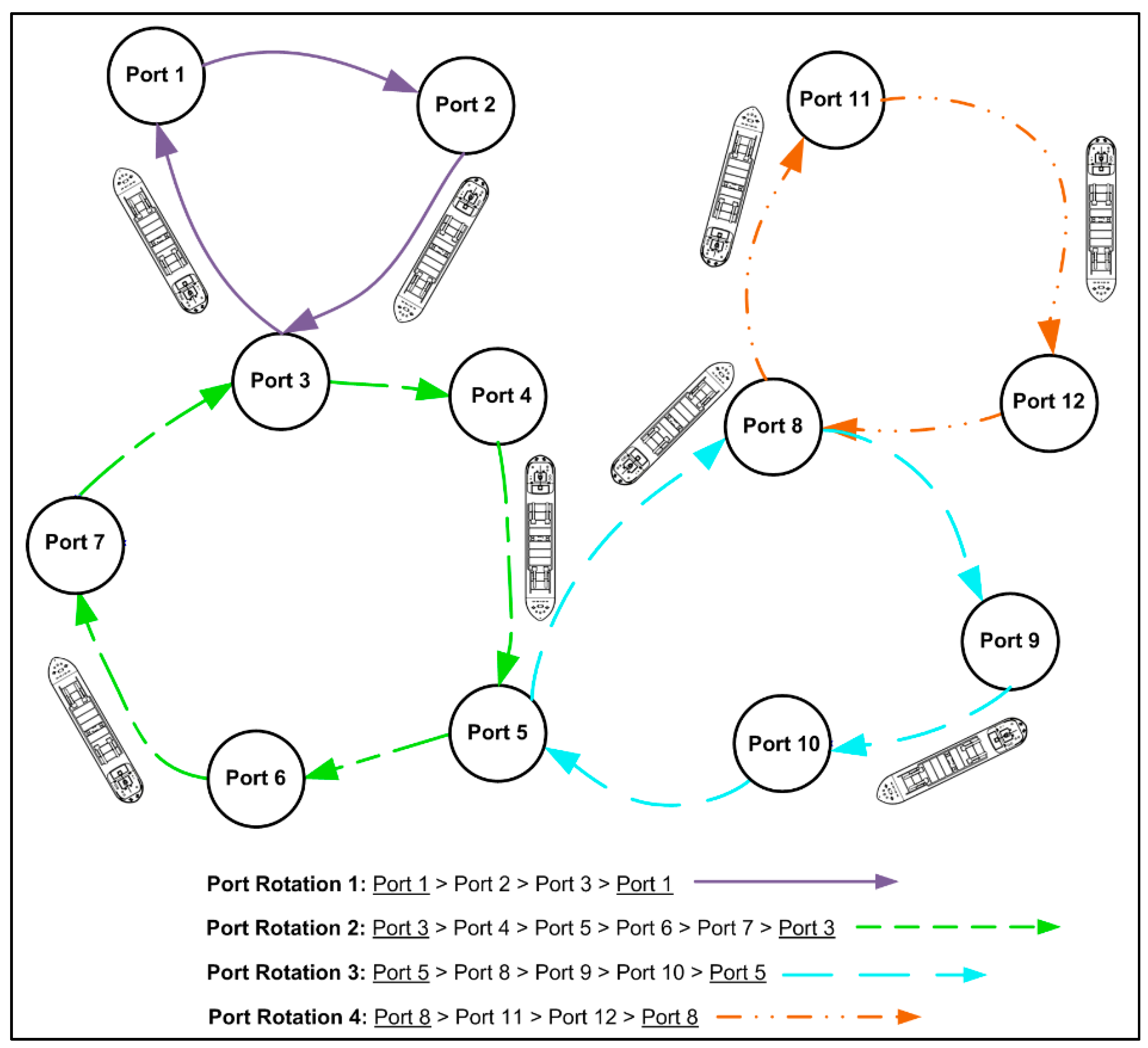
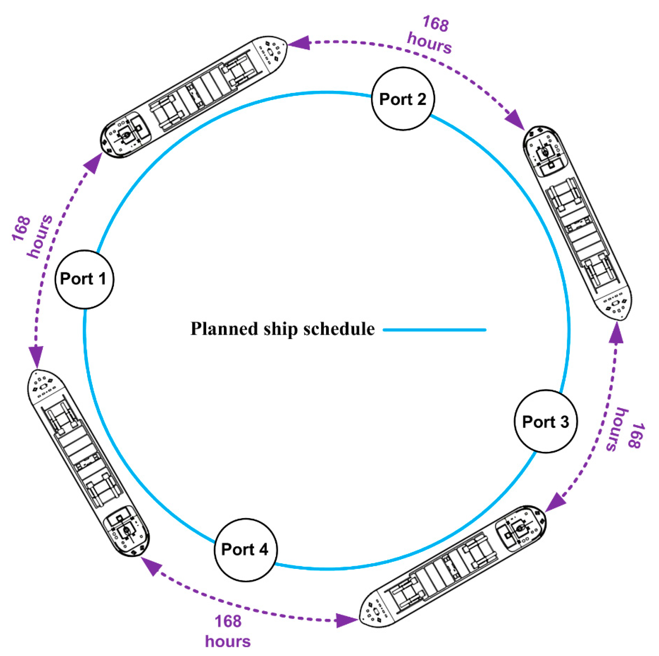
3.1.1. Liner Shipping Route and Ship Voyage

Liner shipping routes (or port rotations) are used by shipping lines to transfer containers from one port to another. A set of ports for a given liner shipping route will be denoted as $P=\left\{1,\dots ,n^1\right\}$ in this study. A liner shipping route can be managed by a single shipping line or several shipping lines (in other words, by a shipping alliance). Each liner shipping route is associated with a pre-determined service frequency, where ships have to visit each port and load/offload containers after a certain number of days. The number of ships that should be allocated for service of a shipping route is proportional to the port service frequency, i.e., more ships should be allocated to the routes that have higher port service frequency (see Section 3.1.4 for more details). After making a round-trip voyage, each ship should return to the first port of call, where the voyage originated. Figure 4 displays a possible liner shipping network with four port rotations. Port rotation “1” includes three ports, port rotation “2” includes five ports, whereas port rotations “3” and “4” are represented by four ports each. In case of port rotation “3”, each ship begins its voyage at port “5”, then visits ports “8”, “9”, “10”, and returns again to port “5” to complete its voyage. Ships sail between consecutive ports along voyage legs (i.e., voyage leg $p$ is used to connect ports $p$ and $p+1$). In case of port rotation “3”, the allocated ships are assumed to sail along voyage leg “8” to reach port “9” from port “8”. Ships may visit a given port more than once during a given voyage.

3.1.2. Ship Service at Ports

Ports of each liner shipping route are generally visited with a particular frequency. Weekly and bi-weekly port visits are viewed as common in the liner shipping industry [32,33,50,51]. Each shipping line has a public schedule of port visits. Service of ships at ports of call is associated with various operations, including the following: (1) transfer of arrived ships to dedicated berthing positions by tug boats; (2) mooring of ships at berthing positions; (3) loading of export containers and offloading of import containers by quay cranes; and (4) transfer of containers between the seaside and the marshaling yard of a marine container terminal. Ships are expected to arrive within a particular time widow (TW) at each port. The arrival TWs are negotiated between the shipping line and each terminal operator. Note that some terminal operators may offer multiple TWs for the arrival of ships, depending on the available ship handling resources and berthing availability [52]. Two attributes are associated with each TW, including the start of the arrival TW at port $p$ (${\mathit{\tau }}_p^{st},p\in P$—hours) and the end of the arrival TW at port $p$ (${\mathit{\tau }}_p^{end},p\in P$—hours).

There are two types of arrival TWs that have been used in the liner shipping literature [53]: (a) hard (or strict) arrival TWs and (b) soft arrival TWs. In case of hard arrival TWs, ships are mandated to arrive within the previously negotiated TWs. In the case of soft TWs, ships are allowed to arrive outside the previously negotiated TWs; however, additional inconvenience costs will be imposed on the shipping line for TW violation. This study assumes TWs to be soft, and a late ship arrival cost (${\kappa }_p^{late},p\in P—$USD/hour) will be imposed for the ships arriving after the end of the negotiated TW. For the ships arriving before the start of the negotiated TW, no penalties will be imposed. However, the ships will have to wait until the start of the negotiated TW. As a part of tactical-level planning of liner shipping operations, along with ship arrival TWs, handling rates have to be negotiated for ships between the shipping line and each terminal operator as well. The handling productivity (measured in number of TEUs loaded/offloaded per hour) is proportional to the handling rate. Let ${\kappa }_p^{hand},p\in P$ represent the unit cost associated with container handling at port $p$ (USD/TEU). As stated in the introduction section of this manuscript, marine terminal operators often experience unexpected disruptive events that cause port congestion, which further affects ship waiting and handling times at ports. Therefore, the ship waiting and handling times, denoted as $\widetilde{{\mathit{\tau }}_p^{wait}},p\in P$ (hours) and $\widetilde{{\mathit{\tau }}_p^{hand}},p\in P$ (hours), respectively, are assumed to be uncertain in this study.

3.1.3. Fuel Consumption Estimation

The fuel cost may comprise a significant portion of the total shipping route service cost. For instance, Ronen [54] reports that the fuel cost can be higher than 75% of the total ship operational costs. Therefore, the amount of fuel required by ships should be accurately estimated for cost-effective ship schedule design. This study assumes that the shipping route will be served by homogeneous ships (i.e., the ships that have similar technical characteristics, including fuel consumption rates). Such an assumption can be viewed as common among the studies on liner shipping operations and ship scheduling [47]. The ship sailing speed and payload are recognized as the major two predictors that dictate the amount of fuel required by ships [15,55,56]. Indeed, ships sailing at higher speeds will require more fuel compared to ships sailing at lower speeds. Furthermore, fully-loaded ships will require more fuel compared to partially-loaded ships. Taking into account the aforementioned considerations, the amount of fuel to be consumed on voyage leg $p$ by the main ship engines (${\mathit{\phi }}_p, p\in P$—tons/nmi) can be computed using the following mathematical relationship:

$${\mathit{\phi }}_p=\frac{\gamma {\left({\mathit{s}}_p\right)}^{\alpha -1}}{24}·{\left(\frac{{\mathit{\delta }}_p^{sea}·\omega +{\delta }^{empty}}{{\delta }^{cap}+{\delta }^{empty}}\right)}^{\frac{2}{3}}\forall p\in P$$

(1)

where: $\alpha ,\gamma$—coefficients associated with the fuel consumption function; ${\mathit{s}}_p,p\in P$—sailing speed of ships on voyage leg $p$ (knots); ${\mathit{\delta }}_p^{sea},p\in P$—number of containers to be carried on voyage leg $p$ (TEUs); $\omega$—average cargo weight within a standard TEU (tons); ${\delta }^{empty}$—weight of a ship without containers (tons); ${\delta }^{cap}$—maximum weight of containers that could be loaded on a ship (tons).

Note that fuel consumption coefficients $\alpha$ and $\gamma$ depend on the ship type. However, the amount of consumed fuel is generally much higher for larger ships that are fully loaded and sail at higher speeds. When selecting the ship sailing speed on each voyage leg of the shipping route, the shipping line has to keep in mind that the maximum ship sailing speed $(s^{max}$—knots) will be dictated by the engine capacity of deployed ships. Moreover, selection of low sailing speeds (i.e., the phenomenon known as “slow steaming”) would reduce fuel consumption and the total fuel cost. However, there is also a minimum sailing speed that could be set for deployed ships ($s^{min}$—knots), as ships sailing at extremely low speeds pose the risk of main engine deterioration [47,55]. Note that Equation (1) is applicable for the fuel consumption by the main ship engines, whereas the fuel consumption by the auxiliary ship engines typically remains constant during the voyage and is accounted for in the ship operational cost.

3.1.4. Port Service Frequency Determination

Determination of the port service frequency is viewed as a tactical-level liner shipping planning decision [43,47]. The port service frequency is set considering the existing demand for export and import containers and is generally set to meet the target profit margins. The shipping line must ensure that the following mathematical relationship is adhered to in order to maintain the port service frequency established [32,33,47]:

$$24·\varphi ·{\mathit{q}}^{tot}={\displaystyle \sum }_{p\in P}{\mathit{\tau }}_p^{sail}+{\displaystyle \sum }_{p\in P}\widetilde{{\mathit{\tau }}_p^{wait}}+{\displaystyle \sum }_{p\in P}\widetilde{{\mathit{\tau }}_p^{hand}}$$

(2)

where: “24”—number of hours for a one-day time interval; $\varphi$—agreed frequency of port service (days); ${\mathit{q}}^{tot}$—number of ships to be deployed (ships); ${\mathit{\tau }}_p^{sail},p\in P$—sailing time of ships on voyage leg $p$ (hours); $\widetilde{{\mathit{\tau }}_p^{wait}},p\in P$—expected waiting time of ships at port $p$ (hours); $\widetilde{{\mathit{\tau }}_p^{hand}},p\in P$—expected handling time of ships at port $p$ (hours).

The left-hand side of Equation (2) is the product of the total number of hours for a one-day time interval, the agreed frequency of port service, and the total number of ships to be deployed. The right-hand side of Equation (2) represents the overall turnaround time of ships, which is estimated as a summation of the overall sailing time of ships, overall expected waiting time of ships at ports, and overall expected handling time of ships at ports. In case the shipping line does not have enough own ships for deployment, additional ships can be charted from other shipping lines in order to ensure the agreed frequency of port service. The following mathematical relationships should be considered by the shipping line when assigning ships for service of a given shipping route:

$${\mathit{q}}^{tot}={\mathit{q}}^{own}+{\mathit{q}}^{char}$$

(3)

$${\mathit{q}}^{own}\le q^{own-max}\mathbf{}$$

(4)

$${\mathit{q}}^{char}\le q^{char-max}\mathbf{}$$

(5)

where: ${\mathit{q}}^{tot}$—number of ships to be deployed (ships); ${\mathit{q}}^{own}—$number of own ships to be deployed (ships); ${\mathit{q}}^{char}$—number of chartered ships to be deployed (ships); $q^{own-max}$—maximum number of own ships that could be deployed (ships); $q^{char-max}$—maximum number of chartered ships that could be deployed (ships).

Chartering of ships from other shipping lines incurs an additional ship chartering cost (${\kappa }^{char}—$USD/day), which is typically higher than the cost associated with operating own ships (${\kappa }^{oper}$—USD/day). To prevent excessive ship chartering costs, the shipping line may decide to increase the ship sailing speed, which will reduce the total ship turnaround time and require fewer ships for deployment. An example of the shipping route service is presented in Figure 5, where a total of four ships are deployed to visit the ports of call. The ships provide weekly port service frequency (i.e., each port is visited every one week or 168 h; $\varphi =7$ days).

3.1.5. Container Inventory Considerations

Sailing speed reduction can assist shipping lines by decreasing the total amount of fuel required for the deployed ships and the total fuel cost as well [57,58,59,60,61]. However, ship sailing speed reduction has certain negative externalities as well. In particular, sailing speed reduction increases the ship transit time and the amount of time containers spend on the ships, which negatively influences the efficiency of liner shipping operations. Therefore, ship schedules should be designed directly taking into consideration container inventory and associated costs. The total cost associated with container inventory (${\mathit{{\rm K}}}^{inv}$—USD) can be computed using the following mathematical relationship [26,32]:

$${\mathit{{\rm K}}}^{inv}={\kappa }^{inv}{\displaystyle \sum }_{p\in P}{\mathit{\delta }}_p^{sea}·{\mathit{\tau }}_p^{sail}$$

(6)

where: ${\kappa }^{inv}$—unit cost associated with container inventory (USD/hour); ${\mathit{\delta }}_p^{sea},p\in P$—number of containers to be carried on voyage leg $p$ (TEUs); ${\mathit{\tau }}_p^{sail},p\in P$—sailing time of a ship on voyage leg $p$ (hours).

3.2. Base Mathematical Model

The base mathematical model for the ship scheduling problem with uncertainties (SSP-U) can be formulated using the objective function (7) and constraints (8) through (26). Note that for a detailed description of all the notations used in the mathematical models presented in this manuscript, interested readers can refer to Appendix A that accompanies this manuscript. The bold notations are used for decision variables, auxiliary variables, and uncertain/stochastic parameters within the mathematical models, whereas the standard font is used for constant parameters. The proposed SSP-U mathematical model assumes that the ship waiting and handling times are uncertain. The SSP-U objective function (7) aims to maximize the total profit ($\mathit{\Pi }$—USD) that will be accumulated by the shipping line from the provided liner shipping service, which is estimated as a difference between the total revenue ($\mathit{R}$—USD) and the total cost associated with the service of the considered shipping route.

$$max \mathit{\Pi }=\left[\mathit{R}-\left({\mathit{{\rm K}}}^{hand}+{\mathit{{\rm K}}}^{late}+{\mathit{{\rm K}}}^{fuel}+{\mathit{{\rm K}}}^{oper}+{\mathit{{\rm K}}}^{char}+{\mathit{{\rm K}}}^{inv}\right)\right]$$

(7)

The total cost associated with the service of the considered shipping route includes the following elements: (1) total cost associated with container handling at ports (${\mathit{{\rm K}}}^{hand}$—USD); (2) total cost associated with late ship arrivals (${\mathit{{\rm K}}}^{late}$—USD); (3) total cost associated with fuel consumption (${\mathit{{\rm K}}}^{fuel}$—USD); (4) total cost associated with basic ship operations (${\mathit{{\rm K}}}^{oper}$—USD); (5) total cost associated with chartering of ships (${\mathit{{\rm K}}}^{char}$—USD); and (6) total cost associated with container inventory (${\mathit{{\rm K}}}^{in\mathrm{v}}$—USD). The SSP-U model includes a total of four groups of constraint sets. The first constraint group, represented by constraints (8) through (11), estimates the sailing time of ships, taking into account the established speed bounds, and the consumption of fuel by the main engines of ships on voyage legs of the considered shipping route. In particular, constraints (8) and (9) assure that the sailing speed of ships remains within the established speed bounds on each voyage leg. Constraints (10) compute the sailing time of ships on each voyage leg based on the voyage leg length and the sailing speed of ships. On the other hand, the consumption of fuel by the main engines of ships on each voyage is computed by constraints (11) based on the sailing speed of ships, coefficients associated with the fuel consumption function, and ship payload.

$${\mathit{s}}_p\le s^{max} \forall p\in P$$

(8)

$${\mathit{s}}_p\ge s^{min} \forall p\in P$$

(9)

$${\mathit{\tau }}_p^{sail}=\frac{l_p}{{\mathit{s}}_p} \forall p\in P$$

(10)

$${\mathit{\phi }}_p=\frac{\gamma {\left({\mathit{s}}_p\right)}^{\alpha -1}}{24}·{\left(\frac{{\mathit{\delta }}_p^{sea}·\omega +{\delta }^{empty}}{{\delta }^{cap}+{\delta }^{empty}}\right)}^{\frac{2}{3}} \forall p\in P$$

(11)

The second constraint group, represented by constraints (12) through (15), estimates the main time components associated with port operations for the considered shipping route. These time components include the following: (1) arrival time of ships at ports (constraints (12) and (13)); (2) late arrival hours of ships at ports (constraints (14)); and (3) departure time of ships from ports (constraints (15)).

$${\mathit{\tau }}_{p+1}^{arr}={\mathit{\tau }}_p^{dep}+{\mathit{\tau }}_p^{sail} \forall p\in P,p<n^1$$

(12)

$${\mathit{\tau }}_1^{arr}={\mathit{\tau }}_p^{dep}+{\mathit{\tau }}_p^{sail}-24·\varphi ·{\mathit{q}}^{tot} \forall p\in P,p=n^1$$

(13)

$${\mathit{\tau }}_p^{late}\ge {\mathit{\tau }}_p^{arr}-{\tau }_p^{end} \forall p\in P$$

(14)

$${\mathit{\tau }}_p^{dep}={\mathit{\tau }}_p^{arr}+\widetilde{{\mathit{\tau }}_p^{wait}}+\widetilde{{\mathit{\tau }}_p^{hand}} \forall p\in P$$

(15)

The third constraint group, represented by constraints (16) through (19), assures that the established frequency of port service will be maintained for the considered shipping route. In particular, constraints (16) assure that the number of ships to be deployed is sufficient for maintaining the established frequency of port service. Constraints (17) compute the number of ships to be deployed based on the number of own ships to be deployed and the number of chartered ships to be deployed. Constraints (18) assure that the number of own ships to be deployed does not exceed the maximum number of own ships that could be deployed for the considered shipping route. Constraints (19) assure that the number of chartered ships to be deployed does not exceed the maximum number of chartered ships that could be deployed for the considered shipping route.

$$24·\varphi ·{\mathit{q}}^{tot}={\displaystyle \sum }_{p\in P}{\mathit{\tau }}_p^{sail}+{\displaystyle \sum }_{p\in P}\widetilde{{\mathit{\tau }}_p^{wait}}+{\displaystyle \sum }_{p\in P}\widetilde{{\mathit{\tau }}_p^{hand}}$$

(16)

$${\mathit{q}}^{tot}={\mathit{q}}^{own}+{\mathit{q}}^{char}$$

(17)

$${\mathit{q}}^{own}\le q^{own-max}$$

(18)

$${\mathit{q}}^{char}\le q^{char-max}$$

(19)

The fourth and the last constraint group, represented by constraints (20) through (26), estimates all the individual cost elements that are required for calculation of the SSP-U objective function (7).

$$\mathit{R}={\displaystyle \sum }_{p\in P}{\kappa }_p^{rev}·{\mathit{\delta }}_p^{port}$$

(20)

$${\mathit{{\rm K}}}^{hand}={\displaystyle \sum }_{p\in P}{\kappa }_p^{hand}·{\mathit{\delta }}_p^{port}$$

(21)

$${\mathit{{\rm K}}}^{late}={\displaystyle \sum }_{p\in P}{\kappa }_p^{late}·{\mathit{\tau }}_p^{late}$$

(22)

$${\mathit{{\rm K}}}^{fuel}={\kappa }^{fuel}{\displaystyle \sum }_{p\in P}{l}_p·{\mathit{\phi }}_p$$

(23)

$${\mathit{{\rm K}}}^{oper}={\kappa }^{oper}·\varphi ·{\mathit{q}}^{own}$$

(24)

$${\mathit{{\rm K}}}^{char}={\kappa }^{char}·\varphi ·{\mathit{q}}^{char}$$

(25)

$${\mathit{{\rm K}}}^{inv}={\kappa }^{inv}{\displaystyle \sum }_{p\in P}{\mathit{\delta }}_p^{sea}·{\mathit{\tau }}_p^{sail}$$

(26)

3.3. Review of the Relevant Studies

With regard to ship scheduling, shipping lines must deal with a key challenge—managing timely liner shipping operations. Customers may face increased logistics costs as a result of lengthier waiting periods and delays because of unreliable ship schedules. Notteboom [11] aimed to understand the causes of unreliability in liner shipping services along with the measures that could be taken to improve the reliability of liner shipping services, such as increasing ship size, rearranging the order of ports, port skipping, and adjusting the sailing speed. Vernimmen et al. [62] explored the reasons for the unreliability of liner schedules and the effects they have on the various stakeholders in the supply chain, such as shipping lines, inland transport operators, terminal operators, and shippers. An example case study showed that a manufacturer’s capacity to source replacement components from overseas may be affected by the level of schedule unreliability. Previous research on the planning and scheduling of container ship routes assumed an acute market demand, which is not a viable assumption in the actual world. To address this gap in the state-of-the-art, Chuang et al. [63] suggested a planning model for container ship routes that takes into consideration uncertain market demand, shipping time, and berthing time. Using the fuzzy set theory, the article developed a genetic algorithm as a decision support system in which the fitness degree of a shipping route was generated from the fuzzy total profit.

Meng and Wang [64] investigated a short-term ship fleet planning problem in liner shipping for a single shipping line, taking container demand uncertainty into account. The problem was addressed using an integer linear mathematical programming model with chance constraints. The objective was to minimize the total route service cost. The developed chance-constraint programming model was solved with CPLEX. A number of research efforts have been dedicated towards a decrease in bunker consumption (and the associated ship emissions). Nonetheless, the studies on ship routing and scheduling have failed to account for the system’s stochastic nature. Qi and Song [65] attempted to fill this gap by developing a mathematical model to reduce fuel consumption while focusing on port time uncertainty. A stochastic approximation strategy based on simulation was used to solve the model. The study also found that reducing the level of service on shorter voyage legs could save fuel consumption. Wang and Meng [7] sought to create a plan that accounts for port operations uncertainties, such as unpredictable waiting times due to port congestion and unknown cargo handling times. The proposed schedule was resilient since it accounted for intrinsic uncertainty in port operations as well as schedule recovery via rapid steaming. In order to address the problem, a mixed-integer stochastic nonlinear programming model was created. The model was then solved using a method that combined a sample average approximation approach, linearization approaches, and a decomposition methodology.

Wang and Meng [66] developed a mixed-integer stochastic nonlinear programming model to maintain the total transit time while minimizing the overall cost. The study explicitly modeled ship fuel consumption, port time uncertainty, and sea contingency. The efficiency of the proposed exact cutting plane-based solution algorithm was validated by extensive computational experiments using realistic data. Di Francesco et al. [67] studied the issue of empty container repositioning in sea transportation networks, taking into account potential uncertainties in port times (e.g., due to various disruptive events). The authors introduced a stochastic programming method that was based on a multi-scenario mathematical model. The provided multi-scenario mathematical approach sought to reduce the total cost. CPLEX was adopted as a solution method. Disruptions are common not just for container shipping, but also for shipping of liquid and dry bulk cargoes. Halvorsen-Weare et al. [68] investigated a real-world liquefied natural gas (LNG) ship scheduling problem, in which the goal was to design robust routes and timetables capturing potential changes in weather circumstances. The study created and tested a solution strategy as well as alternative robustness approaches for scenarios with time horizons ranging from 3 to 12 months. The obtained solutions were evaluated by means of a simulation model in conjunction with a recourse optimization process.

According to Du et al. [69], unexpected severe weather circumstances can have an impact on the voyage of any container ship. Inclement weather, in particular, can have an impact on ship speed and fuel consumption. As a result, the study designed a robust optimization model for the fuel budgeting decision problem, taking into account the influence of severe weather on fuel consumption. To solve the developed mathematical model, a polynomial-time solution methodology was developed. Kepaptsoglou et al. [70] developed a stochastic model to predict the optimum routes for a group of homogeneous container vessels, taking into account sailing time uncertainty caused by severe weather. A chance-constraint formulation was utilized to minimize the total route service cost. A genetic algorithm-based metaheuristic approach was used for the solution. The results of the performed experiments showed that the deployment of a small-size ship fleet was sufficient to provide liner shipping services, even in the presence of small operational delays.

Slow steaming has been widely adopted as an operating approach by shipping lines, since it has proved the efficiency in terms of fuel expense savings. According to the study by Lee et al. [71], slow steaming has certain negative effects as well, primarily increased transit time and unpredictability during the ship voyage. The authors provided a mathematical model for analyzing the links between three important shipping attributes: total bunker cost, shipping time, and cargo delivery reliability. Because of the use of slow steaming, the port time was modeled to be uncertain. Uncertainty in container shipping demand was indicated to be one of the primary concerns that must be accounted for. Ng [72] investigated a container ship deployment problem with stochastic dependencies in container shipping demand, where the variance and mean of the maximum container demand were required to be known. The objective function attempted to minimize the total route service cost. CPLEX was used to solve the mathematical formulation.

Uncertain port service and sailing times owing to bad weather could have a significant impact on ship timetables, particularly during the winter season. Norlund et al. [73] suggested a simulation-optimization-based framework for weekly supply ship scheduling that takes into account the cost, emission, and robustness factors. The goal was to reduce the overall route service cost. It was demonstrated that a greater emphasis on robustness was predicted to result in higher costs and emissions during the winter season. Song et al. [74] focused on liner shipping scheduling under port time uncertainty. The tactical problem aimed to optimize the shipping emission, service reliability, and planned cost. A non-dominated sorting genetic algorithm II (NSGA-II) was applied to solve the model. Based on the numerical results, the deployment of larger ships could be an effective approach to address the uncertain demand. However, it could be an expensive choice because larger ships have higher operational costs.

Wang [75] stated that a series of container ships may not have the same capacity. As a result, the order in which ships arrive affects the number of stacked and delayed containers at ports. The study thus tried to identify the sequence of ships in a string in order to minimize the overall container delay. Experiments revealed that improving ship sequences might save the world’s liner services $6 million per year. Aydin et al. [76] investigated a liner shipping speed optimization and bunkering problem characterized by uncertain port times, with the goal of minimizing fuel consumption while maintaining schedule consistency. The study formulated a dynamic programming model for the decision problem considered. Numerical experiments using real-world data revealed a considerable reduction in fuel consumption when compared to the state-of-the-art approaches. Song et al. [77] aimed to optimize service scheduling, ship sailing speed, and ship deployment in a liner shipping service with port and sea uncertainty. Three service-reliability key performance indicators (KPIs) and two cost-related KPIs were defined. The two cost KPIs represented the shipper and the carrier, whereas the three reliability KPIs represented the terminal operator, the shipper, and the carrier. To solve the provided multi-objective mathematical model, a multi-objective metaheuristic algorithm was used in the study.

Ng and Lin [78] addressed the ship fleet deployment problem in liner shipping, highlighting that only conditional information on container shipping demand could be available. A mathematical formulation was devised with the objective of minimizing the total route service cost. CPLEX was used to solve the developed mathematical formulation. In contrast to road and rail transportation, inland shipping is gaining popularity as a more environmentally friendly and sustainable means of transportation. However, in order to compete in the shipping industry, an inland shipping company must provide a rapid, stable, and cost-effective service. Nonetheless, varying stream flow speeds between ports and uncertain transit times induced by dam lock operations could make the inland ship schedule design difficult. Tan et al. [79] devised a joint ship schedule and speed optimization problem while accounting for uncertainty in dam transit time. A bi-objective chance constraint programming model was then created, with the goal of minimizing both fuel consumption and ship total travel time.

Gurel and Shadmand [80] investigated a liner ship scheduling problem with a heterogeneous fleet while accounting for port handling and waiting time uncertainty in order to minimize fuel consumption. A chance-constrained nonlinear mixed-integer programming model was used to solve the problem. The experimental results indicated that assigning various service levels to port–ship type pairs was more efficient than assigning equal service levels to all pairs. In order to develop new mathematical models for liner shipping service design, Tierney et al. [81] used empirical ship travel time data from a real liner shipping network. In particular, the study proposed three mathematical models, including the following: (1) the design speed model; (2) the optimized speed model; and (3) the optimal speed with maximum transit time model. The models used a buffer time to meet the desired level of service for customers. The proposed models were the first to integrate the support for variable ship speeds in the service design. Using the model for tactical decision support, the researchers showed that it could be used not only for service design but also in negotiations with customers concerning maximum demand transit times and costs.

The study by Liu et al. [82] focused on liner ship speed optimization and bunkering under uncertain container demand. This problem was approached using nonlinear programming and a two-stage stochastic model. The complex bunker consumption function was approximated using piecewise linear functions to reduce the problem’s complexity. The resulting model was then solved using an L-shaped approach, a sample average approximation based on scenario reduction, and a classic sample average approximation. The L-shape technique was found to be more advantageous in terms of both solution quality and computation time. Ding and Xie [83] suggested a two-stage stochastic nonlinear integer programming approach for liner ship scheduling and routing with unexpected shipping delays. The combination of schedule-sensitive shipping demand and unpredictable arrival time factors resulted in a nonlinear model formulation. Nominal delay variables were introduced to the model to produce a comparable linear integer programming counterpart. A Bender’s decomposition method was utilized to solve the linearized problem.

Liu et al. [84] introduced a ship scheduling technique with full voyage constraints to increase the efficiency of operating out-wharf and in-wharf ships at seaports, while taking into account the characteristics of uncertain ship speeds. The study was able to simplify the mathematical model with the use of multi-time restrictions by selecting the minimal safe time intervals. To propose a method for determining the passable time window, the time window concept was linked with the tide height and ship drafts. Additionally, nonlinear global constraints were discretely converted into linear constraints. The developed genetic algorithm sought to reduce the average waiting time for the modified vessel scheduling problem. According to the findings, the reformulated and simplified mathematical model had a lower relative error than conventional priority scheduling rules and could be utilized to successfully boost ship scheduling efficiency while still ensuring traffic safety.

3.4. Literature Summary and Research Gaps

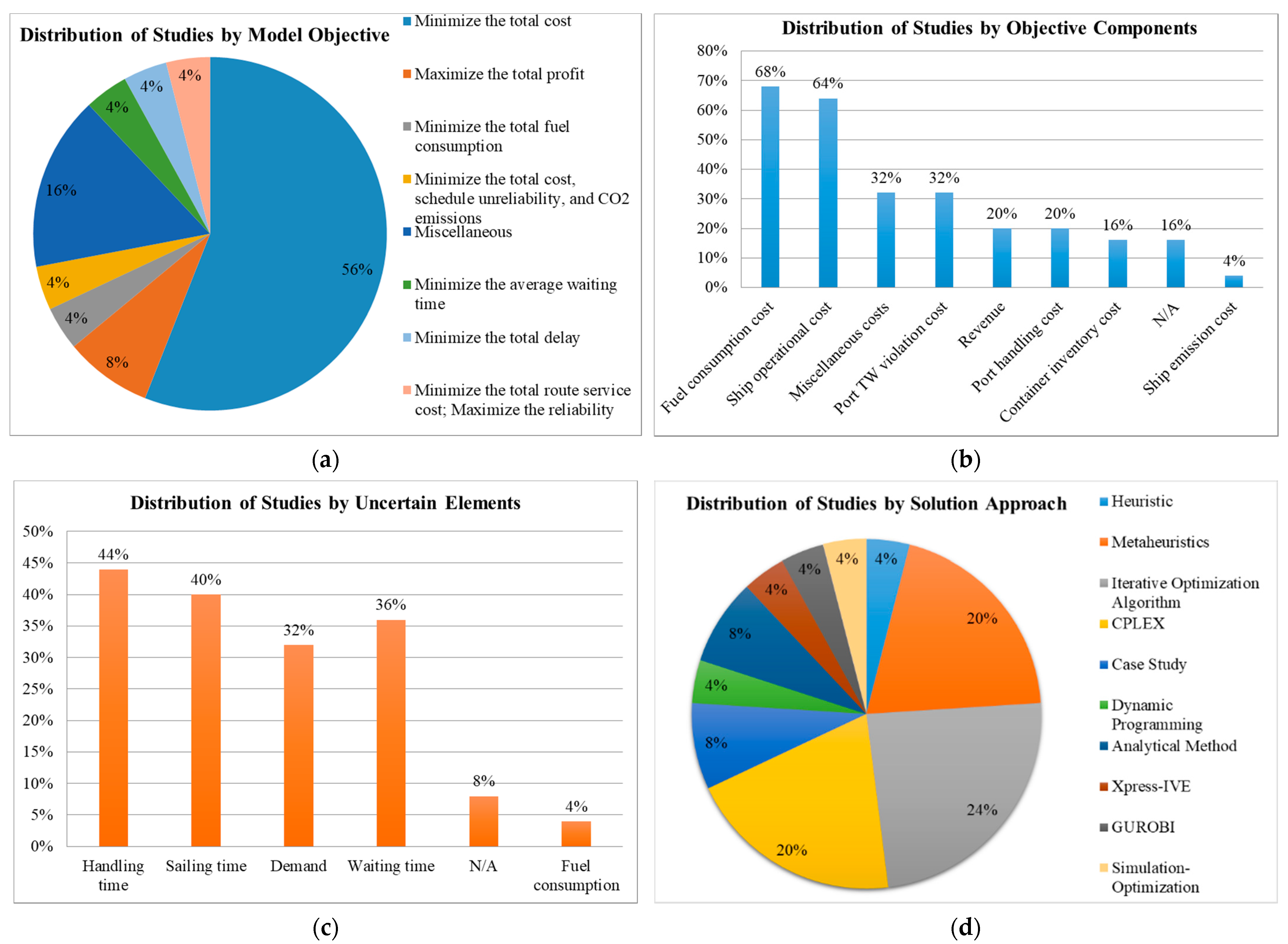
3.4.1. Summary of Findings

A detailed summary of the reviewed studies on uncertainties in liner shipping operations is presented in

Table 1. Summary of the reviewed studies on uncertainties in liner shipping operations.

a/a	Authors	Sailing Speed	Port Time	Objective	Objective Components	Uncertain Elements	Solution Approach	Notes/Important Considerations
1	Notteboom (2006) [11]	N/A	N/A	Assess the causes that might influence the reliability of shipping services between Northern Europe and East Asia	N/A	N/A	Case Study	Reliability of ship schedules
2	Vernimmen et al. (2007) [62]	N/A	N/A	Assess the causes of liner schedule unreliability and how these causes could impact supply chain players	N/A	N/A	Case Study	Reliability of ship schedules
3	Chuang et al. (2010) [63]	U	U	Total profit maximization	REV; TFC; TOC; TPC	Handling time; Sailing time; Container demand	Metaheuristic	Proposing a fuzzy Genetic Algorithm for liner shipping planning
4	Meng and Wang (2010) [64]	F	U	Total route service cost minimization	MSC; REV; TOC	Container demand	CPLEX	Ship fleet planning with uncertainty in container demand
5	Qi and Song (2012) [65]	V	U	Total route service cost minimization	TFC; TVC	Handling time	Iterative Optimization Algorithm; Sample Average Approximation	Minimizing the total expected fuel consumption (and emissions)
6	Wang and Meng (2012) [7]	V	U	Total route service cost minimization	TFC; TOC; TVC	Waiting time; Handling time	Iterative Optimization Algorithm	Consideration of waiting time and handling time uncertainties due to port congestion
7	Wang and Meng (2012) [66]	U	U	Total route service cost minimization	TFC; TOC	Waiting time; Handling time; Sailing time	Iterative Optimization Algorithm	Sea contingency time and uncertainty in port time
8	Di Francesco et al. (2013) [67]	V	U	Total route service cost minimization	MSC; TIC; TFC; TOC; TPC; TVC	Waiting time; Handling time; Container demand	CPLEX	Consideration of uncertain port service times and empty container repositioning
9	Halvorsen-Weare et al. (2013) [68]	U	U	Total route service cost minimization	MSC; TIC; TFC; TOC; TPC; TVC	Sailing time; Demand	Xpress-IVE	Considered changing weather conditions
10	Du et al. (2015) [69]	U	F	Total fuel consumption minimization	MSC	Fuel consumption	Iterative Optimization Algorithm	Considering the impacts of adverse weather on the total fuel consumption
11	Kepaptsoglou et al. (2015) [70]	U	F	Total route service cost minimization	TFC; TOC; TPC	Sailing time	Metaheuristic	Consideration of potential impacts of severe weather on ship sailing times
12	Lee et al. (2015) [71]	V	U	Analyze the relationship amongst shipping time, bunker cost, and cargo delivery reliability	TFC	Waiting time; Handling time	Analytical Method	Proposed a methodology for ship scheduling with guaranteed reliability of cargo delivery
13	Ng (2015) [72]	F	U	Total route service cost minimization	MSC; REV; TOC	Container demand	CPLEX	Consideration of uncertain shipping demand in ship fleet deployment
14	Norlund et al. (2015) [73]	U	U	Total route service cost minimization	TFC; TOC	Waiting time; Handling time; Sailing time	Simulation-Optimization	Acceptable levels of emissions and costs could be achieved with the adequate robustness level
15	Song et al. (2015) [74]	V	U	Total route service cost minimization; Average schedule unreliability minimization; Annual total CO2 emission minimization	MSC; TEC; TFC; TOC; TPC; TVC	Waiting time; Handling time	Metaheuristic	Developing a method to optimize the multiple objectives simultaneously
16	Wang (2015) [75]	F	U	Total delay minimization	N/A	Container demand	Heuristic	Consideration of heterogeneous fleet and container demand uncertainty
17	Aydin et al. (2017) [76]	V	U	Total route service cost minimization	TFC; TVC	Waiting time; Handling time	Dynamic Programming	Speed bunkering and optimization under port time uncertainty
18	Song et al. (2017) [77]	U	U	Total route service cost minimization; Reliability maximization	MSC; TFC; TIC; TOC; TVC	Waiting time; Handling time; Sailing time	Metaheuristic	A multi-objective model consisted of three service-reliability KPIs and two cost-related KPIs
19	Ng and Lin (2018) [78]	F	U	Total route service cost minimization	MSC; REV; TOC	Container demand	CPLEX	Conditional information was assumed to be available for container demand
20	Tan et al. (2018) [79]	U	F	Total fuel consumption cost minimization; Total ship turnaround time minimization	TFC; TOC	Sailing time	Analytical Method	Joint service schedule design and ship sailing speed optimization problem for inland shipping
21	Gurel and Shadmand (2019) [80]	V	U	Total route service cost minimization	TFC	Waiting time; Handling time	CPLEX	Heterogeneous ship fleet considerations
22	Tierney et al. (2019) [81]	U	V	Total route service cost minimization	TFC; TOC	Sailing time	GUROBI	Ship journey times were examined for a real-life liner shipping network
23	Liu et al. (2020) [82]	V	U	Total route service cost minimization	TFC; TIC; TOC	Container demand	Iterative Optimization Algorithms	Solving liner ship bunkering and speed optimization problem
24	Ding and Xie (2021) [83]	U	V	Total profit maximization	REV; TFC; TOC; TVC	Sailing time	Iterative Optimization Algorithm	Balancing chances of unexpected delays and tight timelines
25	Liu et al. (2021) [84]	U	V	Average waiting time minimization	N/A	Sailing time	Metaheuristic	Introduced the notion of a minimum safety time interval (MSTI) in order to decrease the number of constraints

Notes: Sailing Speed and Port Time [V—Variable; F—Fixed; U—Uncertain]; Objective Components [MSC—Miscellaneous Costs; REV—Total Revenue; TEC—Total Ship Emission Cost; TFC—Total Fuel Consumption Cost; TIC—Total Container Inventory Cost; TOC—Total Ship Operational Cost; TPC—Total Port Handling Cost; TVC—Total Cost Associated with Violation of Port Time Windows].

focusing on the following information: (1) authors; (2) sailing speed assumptions; (3) port time assumptions; (4) objective function adopted; (5) components of the objective function adopted; (6) uncertain elements considered; (7) solution approach deployed; and (8) particular notes along with important study considerations. Furthermore, Figure 6 provides a distribution of the reviewed studies by model objective, objective components, uncertain elements, and solution approach. After a thorough review of the literature on uncertainties in liner shipping operations, it can be concluded that a substantial number of studies assumed the ship sailing speed to be uncertain (a total of 44.0%). On the other hand, 68% of studies modeled uncertain port times, mostly focusing on the port handling time uncertainty (see Table 1).

As for the objective functions adopted, the majority of studies (more than 50%) aimed to minimize the total cost of route service, mainly considering fuel consumption cost, ship operational cost, and port TW violation cost (see Figure 6). Only two studies focused on the total profit maximization [63,83]. The analysis of the reviewed studies also shows that single-objective mathematical formulations were common (see Table 1). Only Song et al. [74], Song et al. [77], and Tan et al. [79] presented multi-objective mathematical formulations. In particular, the study by Song et al. [74] aimed to minimize the total cost of route service, average schedule unreliability, and annual CO₂ emissions. Song et al. [77] developed a multi-objective optimization model, where the first objective minimized the total cost of route service, whereas the second one aimed to maximize the schedule reliability.

On the other hand, Tan et al. [79] proposed a bi-objective model, minimizing the total fuel consumption cost and the total turnaround time of ships. The studies conducted by Notteboom [11] and Vernimmen et al. [62] did not propose any mathematical formulations for modeling uncertainties in liner shipping operations and solely focused on the review of factors that could potentially influence the reliability of liner shipping services. As for the solution methods adopted, iterative optimization algorithms were identified to be the most popular methods for the studies on uncertainties in liner shipping operations (see Figure 6). A total of 20% of studies relied on metaheuristic algorithms. Furthermore, a significant number of research efforts deployed exact optimization solvers (e.g., CPLEX, GUROBI, and Xpress-IVE).

3.4.2. Limitations and Future Research Needs

The research gaps and a number of shortcomings in the existing studies on uncertainties in liner shipping operations have been identified. These shortcomings and the future research that is required to bridge these gaps are as follows:

➢

More detailed and accurate historical data for liner shipping operations are required to model uncertainties associated with the main liner shipping processes and assess various mitigation strategies. The collected historical data can be further used in the development of statistical distributions for uncertain container demand, port time, and sailing time [68,81].

➢

Future studies should concentrate on more detailed modeling of uncertain components in liner shipping operations [74]. For instance, the port time component can be disaggregated into various sub-components (e.g., port waiting time, handling time associated with offloading import containers, handling time associated with loading export containers). The effects of uncertainties can be further assessed for each sub-component.

➢

A detailed evaluation of the existing studies on uncertainties in liner shipping operations indicates that many studies strictly concentrate on one source of uncertainties (i.e., uncertainty in demand or uncertainty in sailing time or uncertainty in port handling time or uncertainty in port waiting time). Holistic models that emulate multiples sources of uncertainties at the same time should be further explored by future studies.

➢

Reliability of liner shipping services can be affected by a variety of factors [11,62], including geographical characteristics, the average age of deployed ships, previous maintenance activities of deployed ships, available handling resources of terminal operators and inland operations, and others. Future research should continue investigating the effects of these factors on liner shipping services and directly consider them for planning purposes.

➢

Innovative policies should be explored to offset the effects of uncertainties in liner shipping operations. Dynamic decision-making policies can be promising [71]. As an example, delays due to uncertainties in sailing time could be mitigated by adjusting the ship sailing speed on consecutive voyage legs of a shipping route. However, the ship sailing speed adjustment decision should be made by taking into account other important operational factors (e.g., the number of remaining ports to be visited in a round voyage; increasing fuel cost due to speeding up the ships).

➢

One of the common limitations in the existing liner shipping studies consists in the fact that the impacts of weather conditions are not directly accounted for when planning ship sailing speed decisions [76]. Future research efforts must focus on the development of models that directly capture the expected weather conditions on voyage legs when making ship sailing speed decisions.

➢

Time-dependent port waiting and handling times should be taken into account in future studies. Waiting and handling times vary significantly at the ports depending on the day of the week and the time of day [80]. Ship arrivals should be planned for the time periods with a lower risk of congestion and port time delays.

➢

Future studies should investigate various alternatives for mitigating the effects of significant delays during a ship voyage. In some instances, port skipping or partial loading/offloading of ships might be a promising decision in order to prevent the propagation of delays throughout the entire liner shipping network [81].

➢

Strict port arrival TWs may not be feasible for shipping routes that often encounter uncertainties. Therefore, explicit modeling of soft arrival TWs, where ships are allowed to arrive outside the previously negotiated TW but penalized for TW violations, could be studied more as a part of future research [81].

➢

It is known that fuel prices fluctuate regularly, and different ships need different types of fuel (e.g., ships sailing inside emission control areas must use low-sulfur fuel—[85,86,87,88,89]). Furthermore, ship sailing speed and fuel consumption are often subject to uncertainties [69]. Therefore, future studies should develop more comprehensive liner shipping operations planning models, which directly capture fuel price fluctuations, ship sailing speed uncertainty (and the associated fuel consumption uncertainty), fuel switching, and effective refueling policies.

4. Ship Schedule Recovery

For many years, operations research (OR) methods have been widely employed in the aviation industry [90,91,92]. Initially, OR was utilized exclusively during the planning phase. However, during the last two decades, OR became popular within the disruption management tools to be used in real time and ensure that the intended airline schedule is executed [92,93]. There are evident parallels between the airline and liner shipping industries [2,94]. Many airline and liner shipping services adopt the hub-and-spoke model for their operations. The operations are planned aiming to minimize the total delays in the delivery of cargo (or passengers in case of planning passenger aircraft operations). A variety of recovery strategies can be used in the airline industry to offset the negative impacts of disruptions, including flight cancellations, adding arcs to discourage deviations from aircraft routing, incorporation of delays, and aircraft flying speed adjustments [95,96,97,98]. Some of the recovery strategies used in the airline industry can be applied in the liner shipping industry as well to effectively respond to disruptive events [99].

This section of the manuscript provides a detailed evaluation of the state-of-the-art in the area of ship schedule recovery. First, a description of a general ship schedule recovery problem is presented. Second, the base mathematical models for the ship schedule recovery problem with various recovery options are formulated (including sailing speed adjustment, handling rate adjustment, port skipping, and port skipping with container diversion). Third, a detailed review of the relevant studies is provided. Fourth, a concise state-of-the-art summary is outlined, and critical research gaps in the area of ship schedule recovery are underlined.

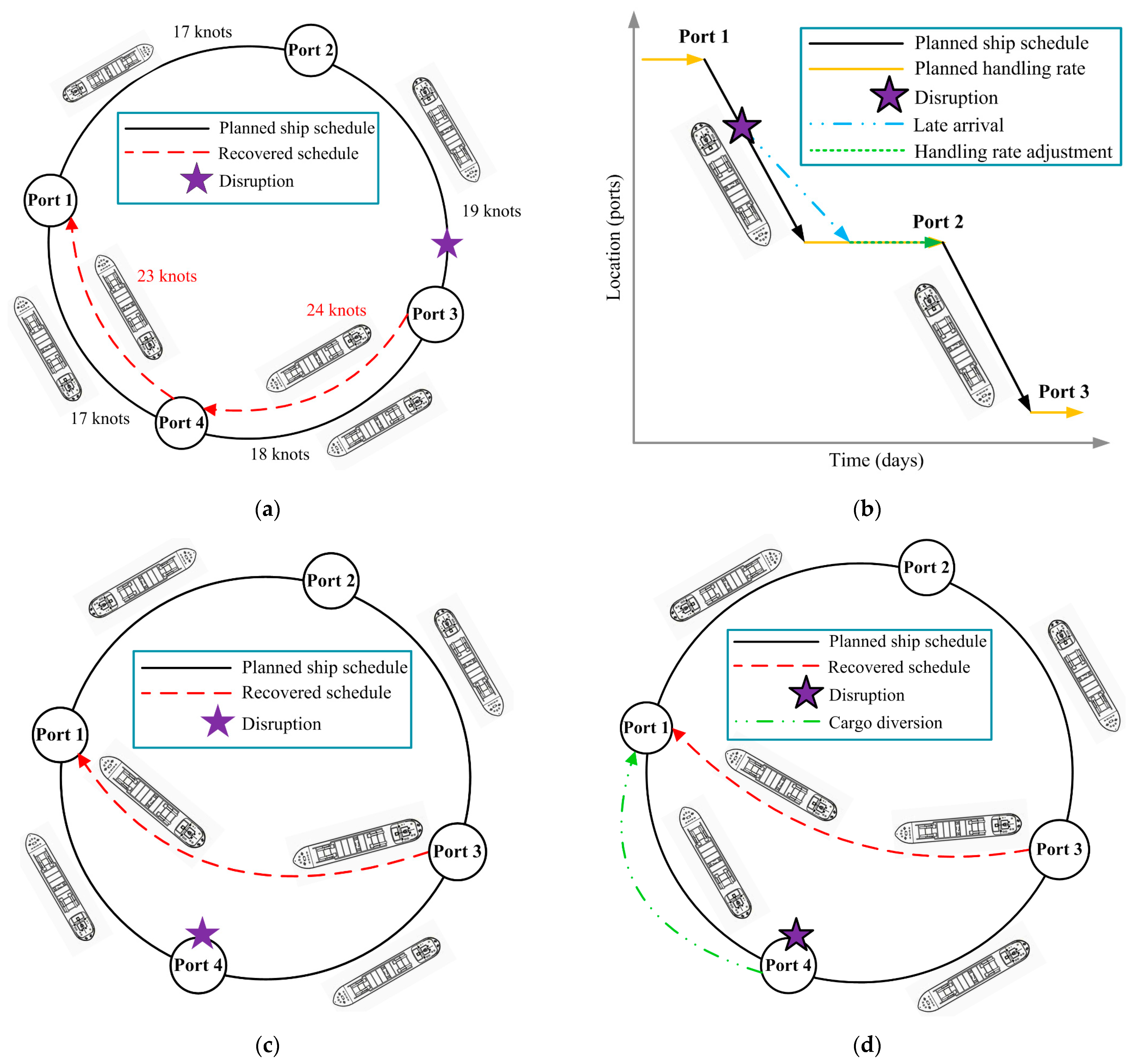
4.1. Problem Description

Unlike the ship schedule design problem, which is viewed as a tactical-level decision problem, the ship schedule recovery problem is an operational level (often real-time) decision problem [43,47]. Therefore, certain components in the ship schedule recovery problem are treated as parameters, not variables that are used in the tactical-level planning models. These components include the following: (1) arrival time of ships at ports for the original ship schedule (${\tau }_p^{arr},p\in P$—hours); (2) number of own ships to be deployed for the original ship schedule $(\overline{q^{own}}$—ships); (3) number of chartered ships to be deployed for the original ship schedule ($\overline{q^{char}}$—ships); (4) number of containers to be handled at ports $(\overline{{\delta }_p^{port}},p\in P$—TEUs); (5) sailing speed of ships on voyage legs for the original ship schedule ($s_p,p\in P$—knots); and (6) total profit that was expected to be accumulated by the shipping line for the original ship schedule (${\Pi }^0$—USD).

Disruptions can occur on voyage legs of the shipping route and/or at ports of call. Let $\widetilde{{\mathit{\tau }}_p^{d-port}},p\in P$ (hours) and $\widetilde{{\mathit{\sigma }}_p^{d-sea}},p\in P$ (knots) be the expected duration for a disruption at port $p$ and the expected change in sailing speed of ships due to a disruption on voyage leg $p$, respectively. In order to offset the effects of disruptions on the ship schedule, the shipping line is assumed to be able to adopt the following ship schedule recovery strategies (see Figure 7): (a) sailing speed adjustment; (b) handling rate adjustment; (c) port skipping; and (d) port skipping and container diversion. An illustrative example of the sailing speed adjustment strategy is showcased in Figure 7a, where a disruptive event happened on the voyage leg connecting ports “2” and “3”. In order to compensate for the delays due to a disruption at sea, the shipping line increased the ship sailing speed on the voyage leg connecting ports “3” and “4” from 18 knots to 24 knots. Moreover, the ship sailing speed was increased from 17 knots to 23 knots on the voyage leg connecting ports “4” and “1” as well. Ship sailing speed adjustment is generally viewed as an effective recovery option to offset small to moderate delays during the voyage but incurs additional fuel costs.

An illustrative example of the handling rate adjustment strategy is showcased in Figure 7b, where a disruptive event happened on the voyage leg connecting ports “1” and “2”. This disruptive event caused a late arrival at port “2”. In order to compensate for the delays due to a disruption at sea, the shipping line requested a handling rate with a higher handling productivity (when compared to the originally negotiated handling rate). Such a recovery option allowed the ship to leave port “2” in a timely manner and sail to port 3” following the original schedule. Handling rate adjustment is generally viewed as an effective recovery option to offset small to moderate delays during the voyage but incurs additional port handling costs (${\kappa }_{ph}^{hand},p\in P, h\in H_p$—USD/TEU, where $H_p=\left\{1,\dots ,n_p^2\right\},p\in P$ is a set of handling rates that can be requested by the shipping line at port $p$). Moreover, selection of this recovery option depends on the handling equipment availability at ports (e.g., some terminal operators may not be able to provide higher handling productivity).

An illustrative example of the port skipping strategy without container diversion is showcased in Figure 7c, where a disruptive event happened at port “4”. The ship was directed to sail from port “3” directly to port “1” without stopping at port “4”, which experienced a disruption. Port skipping is generally viewed as an effective recovery option to offset large delays during the voyage but incurs additional costs due to previously reserved handling equipment (${\kappa }_p^{skip},p\in P$—USD) and misconnected cargo (${\kappa }_p^{mis},p\in P$—USD/TEU).

An illustrative example of the port skipping strategy with container diversion is showcased in Figure 7d, where a disruptive event happened at port “4”. The ship was directed to sail from port “3” directly to port “1” without stopping at port “4”, which experienced a disruption. However, the export containers that had to be loaded at port “4” are diverted to port “1” via the intermodal network. Furthermore, the import containers that had to be offloaded at port “4” can be offloaded at port “1” and delivered to the intended customers via the intermodal network as well. Similar to port skipping, port skipping with container diversion is generally viewed as an effective recovery option to offset large delays during the voyage but incurs additional costs due to previously reserved handling equipment and misconnected cargo. Moreover, the port where the containers will be diverted should have adequate container terminal capacity (${\delta }_p^{term},p\in P$—TEUs) and inland transport capacity (${\delta }_p^{land},p\in P$—TEUs) to ensure that the diverted container demand will be effectively accommodated. Nevertheless, unlike the port skipping strategy, the port skipping strategy with container diversion allows delivery of containers to the intended customers despite port skipping.

4.2. Base Mathematical Models

This section presents the base mathematical models for ship schedule recovery with the following recovery strategies: (a) sailing speed adjustment; (b) handling rate adjustment; (c) port skipping; and (d) port skipping and container diversion.

4.2.1. Sailing Speed Adjustment

The base mathematical model for the ship schedule recovery with sailing speed adjustment (SSR-SSA) can be formulated using the objective function (27) and constraints (28) through (48). The SSR-SSA objective function (27) aims to minimize the total loss of profit that will be endured by the shipping line as a result of disruptions at the considered shipping route. The total profit loss is estimated as a difference between the total profit that was expected to be accumulated by the shipping line for the original ship schedule (${\mathit{\Pi }}^0$—USD) and the total profit that will be accumulated by the shipping line for the recovered schedule of ships ($\overline{\mathit{\Pi }}$—USD).

$$min \left[{\Pi }^0-\overline{\mathit{\Pi }}\right]$$

(27)

The SSR-SSA model includes a total of three groups of constraint sets. The first constraint group, represented by constraints (28) through (32), estimates the recovered sailing time of ships, considering potential sailing speed adjustment to compensate for the effects of disruptions, and the recovered consumption of fuel by the main engines of ships on voyage legs of the considered shipping route. In particular, constraints (28) compute the recovered sailing speed of ships on each voyage leg, considering the expected change in sailing speed of ships due to a disruption and potential ship sailing speed adjustment. Note that constraints (28) assume that the ship sailing speed adjustment strategy could not be implemented on the voyage leg that experienced a disruption. Constraints (29) and (30) assure that the recovered sailing speed of ships remains within the established speed bounds on each voyage leg. Constraints (31) compute the recovered sailing time of ships on each voyage leg based on the voyage leg length and the recovered sailing speed of ships. Constraints (32) calculate the recovered consumption of fuel by the main engines of ships on each voyage based on the recovered sailing speed of ships, coefficients associated with the fuel consumption function, and ship payload.

$$\overline{{\mathit{s}}_p}\le s_p+\widetilde{{\mathit{\sigma }}_p^{d-sea}}·\widetilde{{\mathit{z}}_p^{sea}}+{\mathit{\sigma }}_p^{sea}·\left(1-\widetilde{{\mathit{z}}_p^{sea}}\right) \forall p\in P$$

(28)

$$\overline{{\mathit{s}}_p}\le s^{max} \forall p\in P$$

(29)

$$\overline{{\mathit{s}}_p}\ge s^{min}+\widetilde{{\mathit{\sigma }}_p^{d-sea}}·\widetilde{{\mathit{z}}_p^{sea}} \forall p\in P$$

(30)

$$\overline{{\mathit{\tau }}_p^{sail}}=\frac{l_p}{\overline{{\mathit{s}}_p}} \forall p\in P$$

(31)

$$\overline{{\mathit{\phi }}_p}=\frac{\gamma {\left(\overline{{\mathit{s}}_p}\right)}^{\alpha -1}}{24}·{\left(\frac{{\mathit{\delta }}_p^{sea}·\omega +{\delta }^{empty}}{{\delta }^{cap}+{\delta }^{empty}}\right)}^{\frac{2}{3}} \forall p\in P$$

(32)

The second group of constraints, which is represented by constraints (33) through (40), estimates the main time components associated with port operations that include the following: (1) recovered arrival time of ships at ports (constraints (33) and (34)); (2) recovered handling time of ships at ports (constraints (35)), considering the expected duration of disruptions; (3) recovered waiting time of ships at ports (constraints (36) and (37)); (4) recovered late arrival hours of ships at ports (constraints (38)); (5) recovered departure time of ships from ports (constraints (39)); and (6) turnaround time of ships for the recovered ship schedule (constraints (40)).

$$\overline{{\mathit{\tau }}_{p+1}^{arr}}=\overline{{\mathit{\tau }}_p^{dep}}+\overline{{\mathit{\tau }}_p^{sail}} \forall p\in P,p<n^1$$

(33)

$$\overline{{\mathit{\tau }}_1^{arr}}=\overline{{\mathit{\tau }}_p^{dep}}+\overline{{\mathit{\tau }}_p^{sail}}-\overline{{\mathit{\tau }}^{stt}} \forall p\in P,p=n^1$$

(34)

$$\overline{{\mathit{\tau }}_p^{hand}}=\frac{\overline{{\delta }_p^{port}}}{{\chi }_p}+\widetilde{{\mathit{\tau }}_p^{d-port}}·\widetilde{{\mathit{z}}_p^{port}} \forall p\in P$$

(35)

$$\overline{{\mathit{\tau }}_{p+1}^{wait}}\ge {\tau }_{p+1}^{st}-\overline{{\mathit{\tau }}_p^{dep}}-\overline{{\mathit{\tau }}_p^{sail}} \forall p\in P,p<n^1$$

(36)

$$\overline{{\mathit{\tau }}_1^{wait}}\ge {\tau }_1^{st}-\overline{{\mathit{\tau }}_p^{dep}}-\overline{{\mathit{\tau }}_p^{sail}}+\overline{{\mathit{\tau }}^{stt}} \forall p\in P,p=n^1$$

(37)

$$\overline{{\mathit{\tau }}_p^{late}}\ge \overline{{\mathit{\tau }}_p^{arr}}-{\tau }_p^{arr} \forall p\in P$$

(38)

$$\overline{{\mathit{\tau }}_p^{dep}}=\overline{{\mathit{\tau }}_p^{arr}}+\overline{{\mathit{\tau }}_p^{wait}}+\overline{{\mathit{\tau }}_p^{hand}} \forall p\in P$$

(39)

$$\overline{{\mathit{\tau }}^{stt}}={\displaystyle \sum }_{p\in P}\overline{{\mathit{\tau }}_p^{sail}}+{\displaystyle \sum }_{p\in P}\overline{{\mathit{\tau }}_p^{wait}}+{\displaystyle \sum }_{p\in P}\overline{{\mathit{\tau }}_p^{hand}}$$

(40)

The third and the last constraint group, represented by constraints (41) through (48), estimates all the individual cost elements of the recovered schedule of ships that are required for calculation of the SSR-SSA objective function (27), including the following: (1) total revenue that will be accumulated by the shipping line ($\overline{R}$—USD); (2) total cost associated with container handling at ports ($\overline{{{\rm K}}^{hand}}$—USD); (3) total cost associated with late ship arrivals ($\overline{{\mathit{{\rm K}}}^{late}}$—USD); (4) total cost associated with fuel consumption ($\overline{{\mathit{{\rm K}}}^{fuel}}$—USD); (5) total cost associated with basic ship operations ($\overline{{{\rm K}}^{oper}}$—USD); (6); total cost associated with chartering of ships ($\overline{{{\rm K}}^{char}}$—USD); (7) total cost associated with container inventory ($\overline{{\mathit{{\rm K}}}^{inv}}$—USD); and (8) total profit that will be accumulated by the shipping line ($\overline{\mathit{\Pi }}$—USD).

$$\overline{R}={\displaystyle \sum }_{p\in P}{\kappa }_p^{rev}·\overline{{\delta }_p^{port}}$$

(41)

$$\overline{{{\rm K}}^{hand}}={\displaystyle \sum }_{p\in P}{\kappa }_p^{hand}·\overline{{\delta }_p^{port}}$$

(42)

$$\overline{{\mathit{{\rm K}}}^{late}}={\displaystyle \sum }_{p\in P}{\kappa }_p^{late}·\overline{{\mathit{\tau }}_p^{late}}$$

(43)

$$\overline{{\mathit{{\rm K}}}^{fuel}}=c^{fuel}{\displaystyle \sum }_{p\in P}{l}_p·\overline{{\mathit{\phi }}_p}$$

(44)

$$\overline{{{\rm K}}^{oper}}={\kappa }^{oper}·\varphi ·\overline{q^{own}}$$

(45)

$$\overline{{{\rm K}}^{char}}={\kappa }^{char}·\varphi ·\overline{q^{char}}$$

(46)

$$\overline{{\mathit{{\rm K}}}^{inv}}={\kappa }^{inv}{\displaystyle \sum }_{p\in P}{\mathit{\delta }}_p^{sea}·\overline{{\mathit{\tau }}_p^{sail}}$$

(47)

$$\overline{\mathit{\Pi }}=\left[\overline{R}-\left(\overline{{{\rm K}}^{hand}}+\overline{{\mathit{{\rm K}}}^{late}}+\overline{{\mathit{{\rm K}}}^{fuel}}+\overline{{{\rm K}}^{oper}}+\overline{{{\rm K}}^{char}}+\overline{{\mathit{{\rm K}}}^{inv}}\right)\right]$$

(48)

4.2.2. Handling Rate Adjustment

The base mathematical model for the ship schedule recovery with handling rate adjustment (SSR-HRA) can be formulated using the objective function (49) and constraints (29)–(34), (36)–(41), (43)–(47), and (50)–(54). Similar to the SSR-SSA mathematical model, the SSR-HRA objective function (49) aims to minimize the total loss of profit that will be endured by the shipping line as a result of disruptions at the considered shipping route. The total profit loss is estimated as a difference between the total profit that was expected to be accumulated by the shipping line for the original ship schedule (${\Pi }^0$—USD) and the total profit that will be accumulated by the shipping line for the recovered schedule of ships ($\overline{\mathit{\Pi }}$—USD).

$$min \left[{\Pi }^0-\overline{\mathit{\Pi }}\right]$$

(49)

Constraints (50) compute the recovered sailing speed of ships on each voyage leg, considering the expected change in sailing speed of ships due to a disruption. Constraints (51) assure that only one handling rate will be chosen at each port to serve the arriving ships. Constraints (52) calculate the recovered handling time of ships at ports, considering the expected duration of disruptions and potential handling rate adjustment to compensate for the effects of disruptions. Constraints (53) estimate the total cost associated with container handling at ports for the recovered schedule of ships, considering potential handling rate adjustments at ports. Constraints (54) calculate the total profit that will be accumulated by the shipping line for the recovered schedule of ships, considering potential handling rate adjustments at ports.

$$\overline{{\mathit{s}}_p}\le s_p+\widetilde{{\mathit{\sigma }}_p^{d-sea}}·\widetilde{{\mathit{z}}_p^{sea}} \forall p\in P$$

(50)

$${\displaystyle \sum }_{h\in H_p}{\mathit{x}}_{ph}=1 \forall p\in P$$

(51)

$$\overline{{\mathit{\tau }}_p^{hand}}={\displaystyle \sum }_{h\in H_p}\left(\frac{\overline{{\delta }_p^{port}}}{{\chi }_{ph}}\right)·{\mathit{x}}_{ph}+\widetilde{{\mathit{\tau }}_p^{d-port}}·\widetilde{{\mathit{z}}_p^{port}} \forall p\in P$$

(52)

$$\overline{{\mathit{{\rm K}}}^{hand}}={\displaystyle \sum }_{p\in P}{\displaystyle \sum }_{h\in H_p}{\kappa }_{ph}^{hand}·{\mathit{x}}_{ph}·\overline{{\delta }_p^{port}}$$

(53)

$$\overline{\mathit{\Pi }}=\left[\overline{R}-\left(\overline{{\mathit{{\rm K}}}^{hand}}+\overline{{\mathit{{\rm K}}}^{late}}+\overline{{\mathit{{\rm K}}}^{fuel}}+\overline{{{\rm K}}^{oper}}+\overline{{{\rm K}}^{char}}+\overline{{\mathit{{\rm K}}}^{inv}}\right)\right]$$

(54)

4.2.3. Port Skipping

The base mathematical model for the ship schedule recovery with port skipping (SSR-PS) can be formulated using the objective function (55) and constraints (29)–(34), (36)–(40), (43)–(47), and (56)–(62). Similar to the SSR-SSA mathematical model, the SSR-PS objective function (55) aims to minimize the total loss of profit that will be endured by the shipping line as a result of disruptions at the considered shipping route. The total profit loss is estimated as a difference between the total profit that was expected to be accumulated by the shipping line for the original ship schedule (${\Pi }^0$—USD) and the total profit that will be accumulated by the shipping line for the recovered schedule of ships ($\overline{\mathit{\Pi }}$—USD).

$$min \left[{\Pi }^0-\overline{\mathit{\Pi }}\right]$$

(55)

Constraints (56) compute the recovered sailing speed of ships on each voyage leg, considering the expected change in sailing speed of ships due to a disruption. Constraints (57) assure that a port could be potentially skipped by the shipping line if and only if a disruption happened at that port. Constraints (58) assure that a port could be potentially skipped by the shipping line if and only if the port skipping strategy would be a feasible option for that port. Constraints (59) calculate the recovered handling time of ships at ports, considering the expected duration of disruptions and potential port skipping to compensate for the effects of disruptions. Constraints (60) estimate the total revenue that will be accumulated by the shipping line for the recovered schedule of ships, considering potential port skipping. Constraints (61) compute the total cost associated with container handling at ports for the recovered schedule of ships, considering potential port skipping. Constraints (62) calculate the total profit that will be accumulated by the shipping line for the recovered schedule of ships, considering potential port skipping.

$$\overline{{\mathit{s}}_p}\le s_p+\widetilde{{\mathit{\sigma }}_p^{d-sea}}·\widetilde{{\mathit{z}}_p^{sea}} \forall p\in P$$

(56)

$${\mathit{x}}_p^{skip}\le \widetilde{{\mathit{z}}_p^{port}} \forall p\in P$$

(57)

$${\mathit{x}}_p^{skip}\le z_p^{skip} \forall p\in P$$

(58)

$$\overline{{\mathit{\tau }}_p^{hand}}=\left(\frac{\overline{{\delta }_p^{port}}}{{\chi }_p}+\widetilde{{\mathit{\tau }}_p^{d-port}}·\widetilde{{\mathit{z}}_p^{port}}\right)·\left(1-{\mathit{x}}_p^{skip}\right) \forall p\in P$$

(59)

$$\overline{\mathit{R}}={\displaystyle \sum }_{p\in P}{\kappa }_p^{rev}·\overline{{\delta }_p^{port}}·\left(1-{\mathit{x}}_p^{skip}\right)$$

(60)

$$\overline{{\mathit{{\rm K}}}^{hand}}={\displaystyle \sum }_{p\in P}{\kappa }_p^{hand}·\overline{{\delta }_p^{port}}+{\displaystyle \sum }_{p\in P}\left({\kappa }_p^{skip}+{\kappa }_p^{mis}·\overline{{\delta }_p^{port}}\right)·{\mathit{x}}_p^{skip}$$

(61)

$$\overline{\mathit{\Pi }}=\left[\overline{\mathit{R}}-\left(\overline{{\mathit{{\rm K}}}^{hand}}+\overline{{\mathit{{\rm K}}}^{late}}+\overline{{\mathit{{\rm K}}}^{fuel}}+\overline{{{\rm K}}^{oper}}+\overline{{{\rm K}}^{char}}+\overline{{\mathit{{\rm K}}}^{inv}}\right)\right]$$

(62)

4.2.4. Port Skipping and Container Diversion

The base mathematical model for the ship schedule recovery with port skipping and container diversion (SSR-PSCD) can be formulated using the objective function (63) and constraints (29)–(34), (36)–(40), (43)–(47), (56)–(58), and (64)–(74). Similar to the SSR-SSA mathematical model, the SSR-PSCD objective function (63) aims to minimize the total loss of profit that will be endured by the shipping line as a result of disruptions on the considered shipping route. The total profit loss is estimated as a difference between the total profit that was expected to be accumulated by the shipping line for the original ship schedule (${\Pi }^0$—USD) and the total profit that will be accumulated by the shipping line for the recovered schedule of ships ($\overline{\mathit{\Pi }}$—USD).

$$min \left[{\Pi }^0-\overline{\mathit{\Pi }}\right]$$

(63)

Constraints (64) assure that containers could be diverted to alternative ports only from the skipped ports for the considered shipping route. Constraints (65) assure that containers could be diverted from a given port to an alternative port if and only if such a diversion option is feasible. Constraints (66) determine the ports that will handle diverted containers. Constraints (67) compute the number of containers diverted from a given port to an alternative port. Constraints (68) assure that the available container terminal capacity at the alternative port is sufficient for accommodating the containers diverted. Constraints (69) assure that the available inland transport capacity at the alternative port is sufficient for accommodating the containers diverted. Constraints (70) calculate the recovered handling time of ships at ports, considering the expected duration of disruptions and potential port skipping with container diversion to compensate for the effects of disruptions. Constraints (71) estimate the total revenue that will be accumulated by the shipping line for the recovered schedule of ships, considering potential port skipping and container diversion. Constraints (72) compute the total cost associated with container handling at ports for the recovered schedule of ships, considering potential port skipping and container diversion. Constraints (73) calculate the total cost associated with container diversion for the recovered schedule of ships. Constraints (74) calculate the total profit that will be accumulated by the shipping line for the recovered schedule of ships, considering potential port skipping and container diversion.

$${\mathit{x}}_{p{p}^{*}}^{div}\le {\mathit{x}}_p^{skip} \forall p,p^{*}\in P,p\ne p^{*}$$

(64)

$${\mathit{x}}_{p{p}^{*}}^{div}\le z_{p{p}^{*}}^{div} \forall p,p^{*}\in P,p\ne p^{*}$$

(65)

$${\mathit{x}}_{p^{*}}^{dd}\le {\displaystyle \sum }_{p\in P:p\ne p^{*}}{\mathit{x}}_{p{p}^{*}}^{div} \forall p^{*}\in P$$

(66)

$${\mathit{\delta }}_{p{p}^{*}}^{div}=\overline{{\delta }_p^{port}}·{\mathit{x}}_{p{p}^{*}}^{div} \forall p,p^{*}\in P,p\ne p^{*}$$

(67)

$${\displaystyle \sum }_{p\in P:p\ne p^{*}}{\mathit{\delta }}_{p{p}^{*}}^{div}\le {\delta }_{p^{*}}^{term}·x_{p^{*}}^{dd} \forall p^{*}\in P$$

(68)

$${\displaystyle \sum }_{p\in P:p\ne p^{*}}{\mathit{\delta }}_{p{p}^{*}}^{div}\le {\delta }_{p^{*}}^{land}·{\mathit{x}}_{p^{*}}^{dd} \forall p^{*}\in P$$

(69)

$$\overline{{\mathit{\tau }}_{p^{*}}^{hand}}=\left[\frac{\left(\overline{{\delta }_{p^{*}}^{port}}+{{\displaystyle \sum }}_{p\in P:p\ne p^{*}}{\mathit{\delta }}_{p{p}^{*}}^{div}\right)}{{\chi }_{p^{*}}}+\widetilde{{\mathit{\tau }}_{p^{*}}^{d-port}}·\widetilde{{\mathit{z}}_{p^{*}}^{port}}\right]·\left(1-{\mathit{x}}_{p^{*}}^{skip}\right) \forall p^{*}\in P$$

(70)

$$\overline{\mathit{R}}={\displaystyle \sum }_{p\in P}{\kappa }_p^{rev}·\overline{{\delta }_p^{port}}·\left(1-{\mathit{x}}_p^{skip}\right)+{\displaystyle \sum }_{p\in P}{\displaystyle \sum }_{p^{*}\in P}{\kappa }_p^{rev}·{\mathit{d}}_{p{p}^{*}}^{div}$$

(71)

$$\overline{{\mathit{{\rm K}}}^{hand}}={\displaystyle \sum }_{p\in P}{\kappa }_p^{hand}·\overline{{\delta }_p^{port}}+{\displaystyle \sum }_{p\in P}\left({\kappa }_p^{skip}+{\kappa }_p^{mis}·\overline{{\delta }_p^{port}}\right)·{\mathit{x}}_p^{skip}$$

(72)

$$\overline{{\mathit{{\rm K}}}^{div}}={\displaystyle \sum }_{p\in P}{\displaystyle \sum }_{p^{*}\in P}\left({\kappa }_{p{p}^{*}}^{d-term}+{\kappa }_{p{p}^{*}}^{d-land}\right)·{\mathit{d}}_{p{p}^{*}}^{div}$$

(73)

$$\overline{\mathit{\Pi }}=\left[\overline{\mathit{R}}-\left(\overline{{\mathit{{\rm K}}}^{hand}}+\overline{{\mathit{{\rm K}}}^{late}}+\overline{{\mathit{{\rm K}}}^{fuel}}+\overline{{{\rm K}}^{oper}}+\overline{{{\rm K}}^{char}}+\overline{{\mathit{{\rm K}}}^{inv}}+\overline{{\mathit{{\rm K}}}^{div}}\right)\right]$$

(74)

4.3. Review of the Relevant Studies

The impacts of diverse disruptions in the port network were analyzed by Paul and Maloni [100], and a real-time analysis was undertaken to adapt to dynamically updated port operations. To reduce port and inventory expenses, the network overall capacity was optimized while taking into account the ocean and inland transit operations. The suggested decision support system could dynamically analyze cargo processing time and port capacity while constantly updating the algorithm using regression-based parametric meta-models. Jones et al. [101] created a modeling tool that could be used to simulate container movements in the USA (both imports and exports) under various disruptive scenarios, such as lengthy delays caused by security checks and port disruptions. The system for import/export routing and recovery analysis (SIERRA) development model simulated container movements between 46 nations and the USA. The model sought to reduce total transportation costs. A series of case studies were provided for a number of disruptive scenarios. The developed methodology was found to be efficient and might serve as a useful planning tool for the stakeholders.

Brouer et al. [99] suggested an optimization-based vessel schedule recovery problem (VSRP). The article showed that the planned VSRP is nondeterministic polynomial time hard (NP-hard). The study investigated four schedule recovery options: (a) adjusting the ship’s sailing speed; (b) integrating sailing and port times; (c) skipping a port where a disruptive incident occurred; and (d) modifying the order of port visits. The model’s performance was evaluated by applying numerous recovery scenarios to four real-life situations using an MIP solver, CPLEX. When compared to real-world recovery strategies, the proposed model was able to provide comparable or even superior solution quality. Li et al. [102] developed an operational recovery approach while taking uncertainty factors into account. Port swapping and port skipping were considered in a dynamic programming framework for major disruptions with longer delays. However, if the disruption was minor, the problem was formulated using nonlinear programming, where the only operational strategy taken was speeding up. Computational experiments were carried out to demonstrate the efficacy of the solution methodology, and the relative errors due to discretizing time units were calculated.

Qi [103] summarized the liner shipping disruption management problem. In the study, two models for recovering ship schedules were presented. The first model was designed to recover a single ship’s schedule, whereas the second model was designed to recover the schedules of multiple ships. The goal was to reduce the total cost of fuel and the total cost of a late ship arrival to a minimum. The following operational actions were considered for ship schedule recovery: (a) adjusting the vessel’s sailing speed; (b) port skipping; and (c) port switching. A solution method based on dynamic programming was then proposed. Fischer et al. [104] focused on dealing with ship fleet deployment disruptions in roll-on roll-off liner shipping. The objective was to minimize the entire route service cost, which included total ship operational costs, total fuel consumption costs, total delay costs, total chartering costs, and total costs due to non-provided service. The following disruption methods were proposed: (1) sailing time increase; (2) early arrival awards; and (3) penalization of risky voyage start timings. As a part of the research, a rolling horizon heuristic algorithm was developed for solving the mathematical model. According to the findings, an inclusion of robustness might significantly cut down shipping costs as well as the associated voyage delays.

Li et al. [9] were the first to suggest a real-time schedule recovery policy that took into consideration regular and irregular uncertainties. The recovery model was designed as a multi-stage stochastic control problem to minimize the delay penalty and fuel cost. Using the backward value iteration, an optimal control policy was found. The optimal control policy attributes were established for both types of uncertainty with and without the earliest handling time constraint. Despite the superiority of the suggested real-time schedule recovery policy in computation, calculating the distribution of disruption events for a given planning horizon in practice still remains challenging. The automatic identification system (AIS) data could be used for planning liner shipping operations. Cheraghchi et al. [94] adopted the AIS data to mine and aggregate ship speeds. A speed-based VSRP was developed to minimize the ship schedule disruption. A multi-objective optimization problem was presented, and Pareto-optimal solutions were found using metaheuristic optimization methods. The three objectives of the study were minimizing the overall delays, reducing financial losses, and increasing the average speed conformity with historical values. The study used three evolutionary multi-objective optimizers (EMOO) to find Pareto-optimal solutions.

Ship schedule recovery and ship delays were the focus of the study by Hasheminia and Jiang [105]. Throughout the research, logistic and probit regression models were utilized to determine whether ship delays were random. The data obtained showed that a ship was less likely to be delayed at the terminal if more activities were scheduled in a short period of time (i.e., up to 3 days) after the ship berthing time window. The study also found that larger cargo ships had a lower chance of terminal delays. Smaller ports with less handling capacity face more uncertainty. The authors emphasized that increasing sailing speed is frequently seen as an unfavorable recovery approach due to significant increases in fuel costs. Liner shipping companies use various techniques to recover from disruptions, such as speeding up the ship to arrive at ports within specific time frames. However, increasing the ship’s speed will cause a higher fuel cost, resulting in conflicting objectives. Cheraghchi et al. [106] proposed a multi-objective optimization problem (and corresponding multi-objective evolutionary algorithms) to address these conflicts. As a result, the calculated Pareto set was used to generate ship route-based speed profiles, allowing the stakeholder to make a flexible tradeoff between the total delay and financial losses. Furthermore, the results of the experiments conducted demonstrated the superiority of the NSGA-II metaheuristic.

Emission control areas, often referred to as “ECAs”, have been established by the International Maritime Organization (IMO), which restricts the types of fuel that ships can use in ECAs and the amounts of emissions they can produce. These IMO regulations complicate the VSRP and were not considered in previous studies. Abioye et al. [107] developed a new mixed-integer nonlinear mathematical model to reduce financial losses for ships passing through emission control zones. The piecewise linear approximation was applied to the mathematical model, and the linearized model was solved by CPLEX. Port skipping and ship speed adjustments were considered as recovery options. Numerical experiments demonstrated that the suggested methodology could reduce the total loss while increasing energy efficiency and environmental sustainability. Mulder and Dekker [108] proposed a framework for determining optimal recovery policies and buffer allocations. Three recovery actions were considered: increasing sailing speed, skipping ports, and taking extreme measures (e.g., a “cut-and-go” action at ports). A mixed-integer programming model and a Markov decision process were used in the study. Due to the commercial solver’s runtime limitations and the dimensionality curse that could occur in larger problems, four various heuristics were used to solve the problem in a limited time frame. The findings indicated that optimizing buffer time allocation reduced the costs by 28.9%.

Shipping companies use buffer time and speed adjustments to ensure that their timetables are reliable despite delays. Mulder et al. [109] developed a method that combined timetable planning and execution. The execution of the timetable was modeled using a stochastic dynamic program (SDP). Two options for recovery were considered: (1) increasing sailing speed; and (2) extreme recovery action. Given the need for efficient timetable execution, the study’s approach sought SDPs with the lowest average long-term costs. A case study was provided based on the Maersk data. When compared to the current timetable, the ideal timetable saved between $4 million and $10 million per route each year. To address the VSRP, Xing and Wang [110] employed disruption management to balance service requirements and recovery costs. The study used three schedule recovery strategies: (1) speeding up and reducing port time; (2) swapping port calls; and (3) skipping a port call. According to the potential impact on customers, the priority of the recovery option tiers decreased sequentially. The study presented a service–cost balance model, which was classified as an MINLP model. The container flow recovery problem (CFRP) was also included in the mathematical model, with the assumption that containers could be moved to the next port call if a given port was skipped. No previous research integrated the VSRP and CFRP. The model was solved using LINGO. The optimal solution was found through computational studies, and the model was solved in minutes for a real-life scenario.

The granulated speed-based vessel schedule recovery problem (G-S-VSRP) is considered a big-data-enabled VSRP. The AIS data can be used to create a multi-objective optimization problem by geo-hashing the route between the ports. The G-S-VSRP aimed to reduce delays and financial losses while increasing speed conformity with historical navigational patterns. Geo-hash mining could analyze thousands of speed variables in the G-S-VSRP, creating a large-scale optimization problem. Traditional multi-objective evolutionary algorithms (MOEAs) would be unable to keep up with the problem’s complexity. A divide-and-conquer method was used by Cheraghchi et al. [111] to improve the MOEA’s performance in large-scale optimization problems. As a result of the research, a novel distributed multiplicative cooperative co-evolutionary algorithm was created. Abioye et al. [112] presented a VSRP that, unlike previous models, took into account various types of recovery actions, such as port skipping with/without container diversion, sailing speed adjustment, and handling rate adjustment. The BARON solver was used to solve the given nonlinear mathematical VSRP model. Several numerical experiments with various disruption events were conducted for the Middle East/Pakistan/India-West Mediterranean route. The results of the analysis provided liner shipping companies with managerial insights into designing more efficient ship schedule recovery plans.

De et al. [113] proposed a novel mathematical model to maximize the overall profit while addressing bunkering port selection, ship scheduling decisions, container operations, and determining the amount of oil to be bunkered at each port. To deal with weather-related delays, various recovery strategies, such as re-routing the ship and port swapping, were considered. The impact of fuel prices and the carbon tax on shipping operations was investigated in terms of the overall operating costs. The study provided important policy insights for shipping company executives in terms of having alternate ship route options in the event of normal or disrupted scenarios. Based on the study by Du et al. [114], a tactical liner shipping schedule design problem was examined under sail and port time uncertainty. Ships could lose speed due to weather conditions, delaying their scheduled arrival times. As an alternative, increasing the ship’s speed-adjustment capability, while increasing fuel consumption, could reduce compensation for late arrivals. The study developed a machine learning-based model to address the above-mentioned constraints on speed adjustment measures. A machine learning-based methodology included speed adjustment, reinforcement learning, and neural network training. The effectiveness of machine learning approaches in shipping optimization was demonstrated by numerical studies, which validated the findings and provided a set of managerial insights.

4.4. Literature Summary and Research Gaps

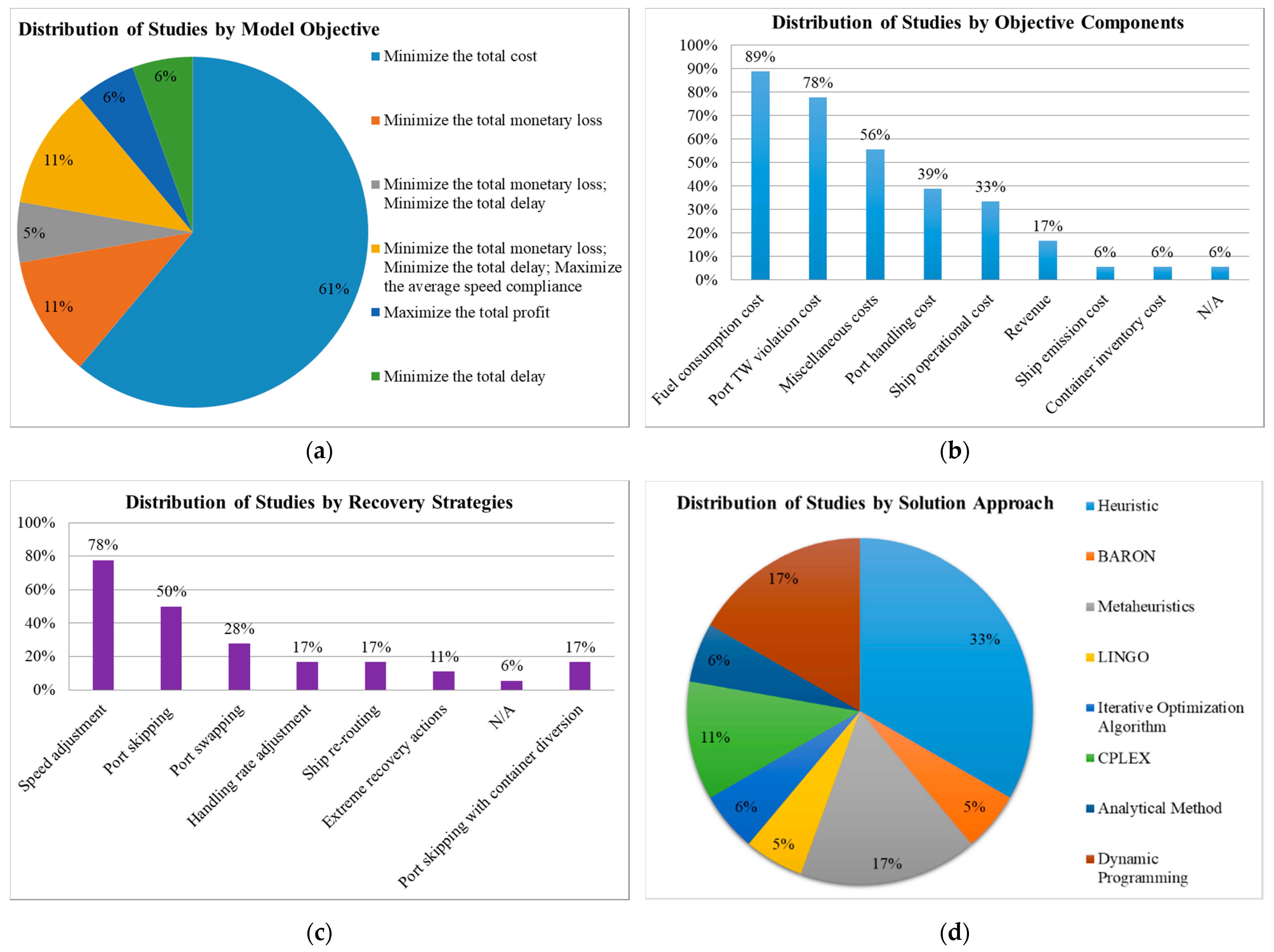
4.4.1. Summary of Findings

A detailed summary of the reviewed studies on ship schedule recovery is presented in

Table 2. Summary of the reviewed studies on ship schedule recovery.

a/a	Authors	Sailing Speed	Port Time	Objective	Objective Components	Recovery Strategies	Solution Approach	Notes/Important Considerations
1	Paul and Maloni (2010) [100]	F	V	Total route service cost minimization	MSC; TFC; TOC; TPC	Ship re-routing	Heuristic	Disruptive event modeling at ports
2	Jones et al. (2011) [101]	V	V	Total cost minimization	MSC	Ship re-routing; Port skipping; Port skipping with container diversion	Heuristic	Proposed a decision support tool to emulate disruptions affecting the USA freight intermodal network
3	Brouer et al. (2013) [99]	V	V	Total route service cost minimization	MSC; TFC; TOC; TPC; TVC	Speed adjustment; Port skipping; Port swapping	CPLEX	Proving the VSRP to be NP-complete
4	Li et al. (2015) [102]	V	V	Total route service cost minimization	TFC; TVC	Speed adjustment; Port skipping; Port swapping	Dynamic Programming	Finding a suitable delay penalty function
5	Qi (2015) [103]	V	V	Total route service cost minimization	TFC; TVC	Speed adjustment; Port skipping; Port swapping	Dynamic Programming	Introduction of two major models, one for a single ship and another one for multiple ships in one network
6	Fischer et al. (2016) [104]	V	F	Total route service cost minimization	MSC; TFC; TOC; TVC	Speed adjustment; Rewards for early arrivals; Penalization of risky voyage start times	Heuristic	Addressing disruptions in the fleet deployment for roll-on roll-off shipping
7	Li et al. (2016) [9]	V	V	Total route service cost minimization	MSC; TFC; TPC; TVC	Speed adjustment; Handling rate adjustment; Port skipping	Dynamic Programming	Considering both regular and unexpected uncertain events
8	Cheraghchi et al. (2017) [94]	V	F	Total monetary loss minimization; Total delay minimization; Average speed compliance maximization	MSC; TFC; TVC	Speed adjustment	Metaheuristics	Ship schedule delays were analyzed using the historical AIS data
9	Hasheminia and Jiang (2017) [105]	V	U	Total delay minimization	N/A	N/A	Analytical Method	Ships with a larger number of containers had a lower risk of delays at the terminal
10	Cheraghchi et al. (2018) [106]	V	F	Total monetary loss minimization; Total delay minimization	TFC; TVC	Speed adjustment	Metaheuristics	Problem evaluation in three scenarios (i.e., scalability analysis, ship steaming policies, and voyage distance analysis)
11	Abioye et al. (2019) [107]	V	V	Total monetary loss minimization	REV; TFC; TIC; TOC; TPC; TVC	Speed adjustment; Port skipping	CPLEX	Capturing enforced regulations within emission control areas
12	Mudler and Dekker (2019) [108]	V	V	Total route service cost minimization	TFC; TVC	Speed adjustment; Port skipping; Extreme recovery actions	Heuristic	Allocation of buffer times
13	Mulder et al. (2019) [109]	V	V	Total route service cost minimization	MSC; TFC; TVC	Speed adjustment; Extreme recovery actions	Iterative Optimization Algorithm	Proposing a method for the integrated development of ship timetables; allocation of buffer times
14	Xing and Wang (2019) [110]	V	V	Total route service cost minimization	MSC; TFC; TPC; TVC	Speed adjustment; Handling rate adjustment; Port swapping; Port skipping without container diversion; Port skipping with container diversion	LINGO	The proposed ship schedule recovery options were categorized into three tiers
15	Cheraghchi et al. (2020) [111]	V	F	Total monetary loss minimization; Total delay minimization; Average speed compliance maximization	MSC; TFC; TVC	Speed adjustment	Metaheuristics	A multi-objective optimization model was developed using the Automatic Identification System (AIS) data
16	Abioye et al. (2021) [112]	V	V	Total monetary loss minimization	MSC; REV; TFC; TOC; TPC; TVC	Speed adjustment; Handling rate adjustment; Port skipping without container diversion; Port skipping with container diversion	BARON	Capturing various realistic scenarios of disruptions
17	De et al. (2021) [113]	V	V	Total profit maximization	REV; TEC; TFC; TPC	Ship re-routing; Port swapping	Heuristic	Deciding on ship scheduling actions and container operations; deciding on the location and amount of marine diesel oil and heavy fuel oil to be bunkered
18	Du et al. (2021) [114]	V	U	Total route service cost minimization	TFC; TOC; TVC	Speed adjustment	Heuristic	Development of a machine learning-based model

Notes: Sailing Speed and Port Time [V—Variable; F—Fixed; U—Uncertain]; Objective Components [MSC—Miscellaneous Costs; REV—Total Revenue; TEC—Total Ship Emission Cost; TFC—Total Fuel Consumption Cost; TIC—Total Container Inventory Cost; TOC—Total Ship Operational Cost; TPC—Total Port Handling Cost; TVC—Total Cost Associated with Violation of Port Time Windows].

focusing on the following information: (1) authors; (2) sailing speed assumptions; (3) port time assumptions; (4) objective function adopted; (5) components of the objective function adopted; (6) recovery strategies considered; (7) solution approach deployed; and (8) particular notes along with important study considerations. Furthermore, Figure 8 provides a distribution of the reviewed studies by model objective, objective components, recovery strategies, and solution approach. After a thorough review of the literature on ship schedule recovery, it can be concluded that the majority of studies assumed the ship sailing speed to be variable (a total of 94.4%). The study by Paul and Maloni [100] mostly focused on modeling disruptions at ports and did not explicitly consider sailing speed adjustment. On the other hand, 66.7% of studies modeled variable port times (see Table 2).

As for the objective functions adopted, the majority of studies (more than 60%) aimed to minimize the total cost of route service, mainly considering fuel consumption cost, port TW violation cost, and port handling cost (see Figure 8). A significant portion of the mathematical models included miscellaneous cost components (e.g., costs incurred due to container diversion, costs due to misconnected cargo as a result of port skipping, costs due to accelerated ship handling at ports). Only one study focused on the total profit maximization [113]. Hasheminia and Jiang [105] investigated the effects of different factors on delays at marine container terminals, aiming to ensure the timely service of ships.

The analysis of the reviewed studies also shows that single-objective mathematical formulations were common (see Table 2). Only Cheraghchi et al. [94], Cheraghchi et al. [106], and Cheraghchi et al. [111] presented multi-objective mathematical formulations. In particular, the studies by Cheraghchi et al. [94] and Cheraghchi et al. [111] aimed to minimize the total monetary losses, minimize the total delay, and maximize the average speed compliance. On the other hand, Cheraghchi et al. [106] presented a bi-objective mathematical model, where the first objective function minimized the total monetary losses, whereas the second objective aimed to minimize the total delay. Sailing speed adjustment and port skipping without container diversion were found to be the most common recovery strategies that were used by the reviewed studies. Extreme recovery actions (e.g., “cut-and-go” when a ship can leave a given port without completing its service) were considered only by two studies, as these actions are not very common in practice. As for the solution methods adopted, heuristics and metaheuristics were found to be the most popular methods for the studies on ship schedule recovery. Furthermore, a significant number of research efforts deployed exact optimization solvers (e.g., CPLEX, LINGO, and BARON).

4.4.2. Limitations and Future Research Needs

The research gaps and a number of shortcomings in the existing studies on ship schedule recovery have been identified. These shortcomings and the future research that is required to bridge these gaps are as follows:

➢

Ship schedule recovery is associated with conflicting decisions. In particular, sailing speed adjustment may allow for partially compensating delays during the voyage and maintaining adequate service levels for customers. However, such a recovery option will increase the amount of required fuel and fuel costs. There is a lack of multi-objective mathematical formulations for ship schedule recovery that are able to assist with the analysis of conflicting objectives [94,106,111]. Future research should focus more on multi-objective ship schedule recovery.

➢

Future studies should concentrate on the development of innovative forecasting methods that could predict the occurrence of disruptive events and their duration [110]. The outcomes from these methods could be further used by shipping lines in the selection of the appropriate recovery strategies and offset the effects of disruptive events.

➢

The shipping industry has been facing many challenges in recent years (e.g., COVID-19), and the cost of ship schedule recovery would add additional pressure on shipping lines. Risk-sharing mechanisms between carriers and shippers should be investigated further in future studies to alleviate the pressure on shipping lines and enable them to maintain a high level of customer service [110].

➢

Sailing speed adjustment can serve as an effective recovery option but incurs additional fuel costs. The fuel consumption of ships depends on some other attributes as well, including previous maintenance activities, ship payload, ship age, and ship geometric characteristics [15,107]. Future research on ship schedule recovery should account for the aforementioned attributes and accurately quantify the amount of required fuel for the recovered ship schedules.

➢

Decentralized decision-making with several shipping lines should be studied more in depth. A freight forwarder, for example, may arrange transshipment between the ships of two different shipping lines. These two shipping lines would coordinate their ship recovery schedules for transshipment in an ideal world. Nevertheless, since each shipping line must minimize its cost function, centralized and optimized scheduling would be difficult to execute in practice. Game-theoretic models for ship schedule recovery in decentralized settings would be suitable in such scenarios [103].

➢

Sailing speed adjustment was identified as the most popular ship schedule recovery strategy. However, sailing speed adjustment alone may not be able to fully offset the effects of a disruptive event. Therefore, future studies should focus on the development of more advanced mathematical models and solution methods that consider a simultaneous implementation of various recovery strategies (e.g., sailing speed adjustment + port skipping or port swapping—[106]).

➢

Certain extreme ship schedule recovery options (e.g., “cut-and-go” when a ship can leave a given port without completing its service) should be better explored by future research efforts to determine the scenarios when these options might be viable and reduce potential monetary losses due to disruptive events.

➢

The effects of disruptions at ports and sea may influence not only shipping lines but other major supply chain players as well, including marine terminal operators, logistics companies, and inland operators [47]. Future mathematical models should evaluate various recovery strategies, considering the entire intermodal network effects—not just ship schedules.

➢

Drones have been widely used for monitoring various assets, including the assessment of infrastructure damages as a result of disruptive events [115,116,117,118,119]. The deployment of drones for the assessment of disruptive events in liner shipping operations should be investigated as a part of future research. Drones can be used to accurately determine the effects of damages to the port infrastructure and the expected duration of port closures.

5. Concluding Remarks

Maritime transportation has been a popular mode of transportation (especially, for the transfer of bulk and containerized cargoes) but often faces different types of disruptions, such as port congestion, labor strikes, severe weather conditions, shipping container shortages, and customs delays. The outbreak of COVID-19 is recognized as a major disruptive event for liner shipping and maritime transportation, which resulted in the closure of certain marine terminals and substantial supply chain disruptions. A large number of studies were dedicated to the planning of different liner shipping operations. Furthermore, a number of survey studies were conducted in the past aiming to provide a holistic overview of the liner shipping literature. Nevertheless, there is still a lack of systematic literature surveys that specifically concentrate on uncertainties in liner shipping operations and ship schedule recovery. Therefore, the present research conducted a comprehensive up-to-date review of the liner shipping literature with a specific emphasis on uncertainties in liner shipping operations and ship schedule recovery. The collected studies were reviewed in a systematic way capturing the main assumptions regarding sailing speed and port time modeling, objective(s) considered, objective function components, uncertain elements, ship schedule recovery options, solution approaches, and specific considerations adopted. Moreover, supporting mathematical formulations were presented along with the major future research needs.

It was found that the reviewed studies mostly aimed to minimize the total cost of route service, primarily considering fuel consumption cost, ship operational cost, and port time window violation cost. A significant number of studies captured uncertainty in port handling time and ship sailing time. Single-objective mathematical formulations were common among the collected studies. A large variety of solution methods were presented for the considered decision problems related to uncertainties in liner shipping operations and ship schedule recovery, including heuristic methods, metaheuristic methods, and exact optimization methods (e.g., CPLEX, GUROBI, and BARON). Sailing speed adjustment and port skipping without container diversion were found to be the most common recovery strategies that were used by the reviewed studies. Extreme recovery actions (e.g., “cut-and-go” when a ship can leave a given port without completing its service) were considered only by a few studies. The outcomes from this research are expected to assist the relevant stakeholders involved in liner shipping operations with improvements in the reliability of their schedules and selection of the appropriate recovery options in response to major disruptive events.

There are several areas for extending the scope of this study that can be explored by future studies. First, a set of detailed interviews could be conducted with the relevant stakeholders involved in liner shipping operations to identify the best practices used to maintain schedule reliability and determine whether these practices receive sufficient attention in the literature. Second, a set of detailed interviews could be conducted with the marine terminal operators and inland operators to better understand how liner shipping disruptions influence terminal operations and identify the best mitigation strategies. Third, the future research needs, which were identified as a part of the performed literature survey, should be prioritized considering the input from the relevant stakeholders. Fourth, a new literature survey could be conducted to better understand the impacts of the COVID-19 pandemic on maritime supply chains. The identified insights could be further used to make maritime supply chains more resilient and be more prepared for the pandemics that may come in the following years.

References

- McLean, C. Government action and the new blue economy. In Preparing a Workforce for the New Blue Economy; Elsevier: Amsterdam, The Netherlands, 2021; pp. 513–525. [Google Scholar]
- Christiansen, M.; Fagerholt, K.; Nygreen, B.; Ronen, D. Maritime transportation. Handb. Oper. Res. Manag. Sci. 2007, 14, 189–284. [Google Scholar]
- Zhang, Y.; Sun, Z. The Coevolutionary Process of Maritime Management of Shipping Industry in the Context of the COVID-19 Pandemic. J. Mar. Sci. Eng. 2021, 9, 1293. [Google Scholar] [CrossRef]
- Zhu, J.; Wang, H.; Xu, J. Fuzzy DEMATEL-QFD for Designing Supply Chain of Shipbuilding Materials Based on Flexible Strategies. J. Mar. Sci. Eng. 2021, 9, 1106. [Google Scholar] [CrossRef]
- Lezhnina, E.A.; Balykina, Y.E. Cooperation between sea ports and carriers in the logistics chain. J. Mar. Sci. Eng. 2021, 9, 774. [Google Scholar] [CrossRef]
- Svanberg, M.; Holm, H.; Cullinane, K. Assessing the Impact of Disruptive Events on Port Performance and Choice: The Case of Gothenburg. J. Mar. Sci. Eng. 2021, 9, 145. [Google Scholar] [CrossRef]
- Wang, S.; Meng, Q. Robust schedule design for liner shipping services. Transp. Res. Part E Logist. Transp. Rev. 2012, 48, 1093–1106. [Google Scholar] [CrossRef]
- How Bad Weather Impacts Shipping (and How to Deal With It). Available online: https://www.icecargo.com.au/weather-impacts-shipping/ (accessed on 1 January 2022).
- Li, C.; Qi, X.; Song, D. Real-time schedule recovery in liner shipping service with regular uncertainties and disruption events. Transp. Res. Part B Methodol. 2016, 93, 762–788. [Google Scholar] [CrossRef]
- Slagen, D. The Operational Guide to Weather Excellence: Intermodal. Available online: https://www.tomorrow.io/blog/the-operational-guide-to-weather-excellence-intermodal/ (accessed on 1 January 2022).
- Notteboom, T.E. The time factor in liner shipping services. Marit. Econ. Logist. 2006, 8, 19–39. [Google Scholar] [CrossRef]
- Dadashi, A.; Dulebenets, M.A.; Golias, M.M.; Sheikholeslami, A. A novel continuous berth scheduling model at multiple marine container terminals with tidal considerations. Marit. Bus. Rev. 2017, 2, 142–157. [Google Scholar] [CrossRef] [Green Version]
- Liu, B.; Li, Z.-C.; Wang, Y.; Sheng, D. Short-term berth planning and ship scheduling for a busy seaport with channel restrictions. Transp. Res. Part E Logist. Transp. Rev. 2021, 154, 102467. [Google Scholar] [CrossRef]
- Review of Maritime Transport. 2020. Available online: https://unctad.org/en/PublicationsLibrary/rmt2020_en.pdf (accessed on 1 January 2022).
- Pasha, J.; Dulebenets, M.A.; Fathollahi-Fard, A.M.; Tian, G.; Lau, Y.-Y.; Singh, P.; Liang, B. An integrated optimization method for tactical-level planning in liner shipping with heterogeneous ship fleet and environmental considerations. Adv. Eng. Inform. 2021, 48, 101299. [Google Scholar] [CrossRef]
- Chen, Q.; Ge, Y.-E.; Lau, Y.-Y.; Dulebenets, M.A.; Sun, X.; Kawasaki, T.; Mellalou, A.; Tao, X. Effects of COVID-19 on passenger shipping activities and emissions: Empirical analysis of passenger ships in Danish waters. Marit. Policy Manag. 2022, 1–21. [Google Scholar] [CrossRef]
- Dulebenets, M.A. Multi-objective collaborative agreements amongst shipping lines and marine terminal operators for sustainable and environmental-friendly ship schedule design. J. Clean. Prod. 2022, 342, 130897. [Google Scholar] [CrossRef]
- Millefiori, L.M.; Braca, P.; Zissis, D.; Spiliopoulos, G.; Marano, S.; Willett, P.K.; Carniel, S. COVID-19 impact on global maritime mobility. Sci. Rep. 2021, 11, 1–16. [Google Scholar]
- Wetzel, D.; Tierney, K. Integrating fleet deployment into liner shipping vessel repositioning. Transp. Res. Part E Logist. Transp. Rev. 2020, 143, 102101. [Google Scholar] [CrossRef]
- Zhang, E.; Chu, F.; Wang, S.; Liu, M.; Sui, Y. Approximation approach for robust vessel fleet deployment problem with ambiguous demands. J. Comb. Optim. 2020, 1–15. [Google Scholar] [CrossRef]
- Zhen, L.; Wu, Y.; Wang, S.; Laporte, G. Green technology adoption for fleet deployment in a shipping network. Transp. Res. Part B Methodol. 2020, 139, 388–410. [Google Scholar] [CrossRef]
- Chen, J.; Zhuang, C.; Yang, C.; Wan, Z.; Zeng, X.; Yao, J. Fleet co-deployment for liner shipping alliance: Vessel pool operation with uncertain demand. Ocean Coast. Manag. 2021, 214, 105923. [Google Scholar] [CrossRef]
- Rodriguez, M.H.; Agrell, P.J.; Manrique-de-Lara-Peñate, C.; Trujillo, L. A multi-criteria fleet deployment model for cost, time and environmental impact. Int. J. Prod. Econ. 2022, 243, 108325. [Google Scholar] [CrossRef]
- Lin, D.-Y.; Tsai, Y.-Y. The ship routing and freight assignment problem for daily frequency operation of maritime liner shipping. Transp. Res. Part E Logist. Transp. Rev. 2014, 67, 52–70. [Google Scholar] [CrossRef]
- Zhang, A.; Lee Lam, J.S. Impacts of schedule reliability and sailing frequency on the liner shipping and port industry: A study of Daily Maersk. Transp. J. 2014, 53, 235–253. [Google Scholar] [CrossRef]
- Giovannini, M.; Psaraftis, H.N. The profit maximizing liner shipping problem with flexible frequencies: Logistical and environmental considerations. Flex. Serv. Manuf. J. 2019, 31, 567–597. [Google Scholar] [CrossRef] [Green Version]
- Pasha, J.; Dulebenets, M.A.; Kavoosi, M.; Abioye, O.F.; Theophilus, O.; Wang, H.; Kampmann, R.; Guo, W. Holistic tactical-level planning in liner shipping: An exact optimization approach. J. Shipp. Trade 2020, 5, 1–35. [Google Scholar] [CrossRef]
- Lee, H.; Aydin, N.; Choi, Y.; Lekhavat, S.; Irani, Z. A decision support system for vessel speed decision in maritime logistics using weather archive big data. Comput. Oper. Res. 2018, 98, 330–342. [Google Scholar] [CrossRef]
- Mallidis, I.; Iakovou, E.; Dekker, R.; Vlachos, D. The impact of slow steaming on the carriers’ and shippers’ costs: The case of a global logistics network. Transp. Res. Part E Logist. Transp. Rev. 2018, 111, 18–39. [Google Scholar] [CrossRef] [Green Version]
- Li, X.; Sun, B.; Guo, C.; Du, W.; Li, Y. Speed optimization of a container ship on a given route considering voluntary speed loss and emissions. Appl. Ocean Res. 2020, 94, 101995. [Google Scholar] [CrossRef]
- Wu, W.-M. The optimal speed in container shipping: Theory and empirical evidence. Transp. Res. Part E Logist. Transp. Rev. 2020, 136, 101903. [Google Scholar] [CrossRef]
- Wang, S.; Alharbi, A.; Davy, P. Liner ship route schedule design with port time windows. Transp. Res. Part C Emerg. Technol. 2014, 41, 1–17. [Google Scholar] [CrossRef] [Green Version]
- Alharbi, A.; Wang, S.; Davy, P. Schedule design for sustainable container supply chain networks with port time windows. Adv. Eng. Inform. 2015, 29, 322–331. [Google Scholar] [CrossRef]
- Dulebenets, M.A. A comprehensive multi-objective optimization model for the vessel scheduling problem in liner shipping. Int. J. Prod. Econ. 2018, 196, 293–318. [Google Scholar] [CrossRef]
- Ozcan, S.; Eliiyi, D.T.; Reinhardt, L.B. Cargo allocation and vessel scheduling on liner shipping with synchronization of transshipments. Appl. Math. Model. 2020, 77, 235–252. [Google Scholar] [CrossRef]
- Zhang, B.; Zheng, Z.; Wang, D. A model and algorithm for vessel scheduling through a two-way tidal channel. Marit. Policy Manag. 2020, 47, 188–202. [Google Scholar] [CrossRef]
- Zheng, J.; Hou, X.; Qi, J.; Yang, L. Liner ship scheduling with time-dependent port charges. Marit. Policy Manag. 2020, 49, 18–38. [Google Scholar] [CrossRef]
- Zhuge, D.; Wang, S.; Zhen, L.; Laporte, G. Schedule design for liner services under vessel speed reduction incentive programs. Nav. Res. Logist. (NRL) 2020, 67, 45–62. [Google Scholar] [CrossRef] [Green Version]
- Dulebenets, M.A. The vessel scheduling problem in a liner shipping route with heterogeneous fleet. Int. J. Civ. Eng. 2018, 16, 19–32. [Google Scholar] [CrossRef]
- Wang, Y.; Wang, S. Deploying, scheduling, and sequencing heterogeneous vessels in a liner container shipping route. Transp. Res. Part E Logist. Transp. Rev. 2021, 151, 102365. [Google Scholar] [CrossRef]
- Zheng, J.; Ma, Y.; Ji, X.; Chen, J. Is the weekly service frequency constraint tight when optimizing ship speeds and fleet size for a liner shipping service? Ocean Coast. Manag. 2021, 212, 105815. [Google Scholar] [CrossRef]
- Pantuso, G.; Fagerholt, K.; Hvattum, L.M. A survey on maritime fleet size and mix problems. Eur. J. Oper. Res. 2014, 235, 341–349. [Google Scholar] [CrossRef] [Green Version]
- Meng, Q.; Wang, S.; Andersson, H.; Thun, K. Containership routing and scheduling in liner shipping: Overview and future research directions. Transp. Sci. 2014, 48, 265–280. [Google Scholar] [CrossRef] [Green Version]
- Wang, S.; Meng, Q. Container liner fleet deployment: A systematic overview. Transp. Res. Part C Emerg. Technol. 2017, 77, 389–404. [Google Scholar] [CrossRef]
- Meng, Q.; Zhao, H.; Wang, Y. Revenue management for container liner shipping services: Critical review and future research directions. Transp. Res. Part E Logist. Transp. Rev. 2019, 128, 280–292. [Google Scholar] [CrossRef]
- Christiansen, M.; Hellsten, E.; Pisinger, D.; Sacramento, D.; Vilhelmsen, C. Liner shipping network design. Eur. J. Oper. Res. 2020, 286, 1–20. [Google Scholar] [CrossRef]
- Dulebenets, M.A.; Pasha, J.; Abioye, O.F.; Kavoosi, M. Vessel scheduling in liner shipping: A critical literature review and future research needs. Flex. Serv. Manuf. J. 2021, 33, 43–106. [Google Scholar] [CrossRef]
- Song, D. A literature review, container shipping supply chain: Planning problems and research opportunities. Logistics 2021, 5, 41. [Google Scholar] [CrossRef]
- Krippendorff, K. Content Analysis: An Introduction to Its Methodology; Sage Publications: Thousand Oaks, CA, USA, 2018. [Google Scholar]
- Dulebenets, M.A. The green vessel scheduling problem with transit time requirements in a liner shipping route with Emission Control Areas. Alex. Eng. J. 2018, 57, 331–342. [Google Scholar] [CrossRef]
- Dulebenets, M.A. Green vessel scheduling in liner shipping: Modeling carbon dioxide emission costs in sea and at ports of call. Int. J. Transp. Sci. Technol. 2018, 7, 26–44. [Google Scholar] [CrossRef]
- Christiansen, M.; Fagerholt, K. Robust ship scheduling with multiple time windows. Nav. Res. Logist. (NRL) 2002, 49, 611–625. [Google Scholar] [CrossRef]
- Fagerholt, K. Ship scheduling with soft time windows: An optimisation based approach. Eur. J. Oper. Res. 2001, 131, 559–571. [Google Scholar] [CrossRef]
- Ronen, D. The effect of oil price on containership speed and fleet size. J. Oper. Res. Soc. 2011, 62, 211–216. [Google Scholar] [CrossRef]
- Psaraftis, H.N.; Kontovas, C.A. Speed models for energy-efficient maritime transportation: A taxonomy. Transp. Res. Part C Emerg. Technol. 2013, 26, 331–351. [Google Scholar] [CrossRef]
- Kontovas, C.A. The green ship routing and scheduling problem (GSRSP): A conceptual approach. Transp. Res. Part D Transp. Environ. 2014, 31, 61–69. [Google Scholar] [CrossRef]
- Ferrari, C.; Parola, F.; Tei, A. Determinants of slow steaming and implications on service patterns. Marit. Policy Manag. 2015, 42, 636–652. [Google Scholar] [CrossRef]
- De, A.; Mamanduru, V.K.R.; Gunasekaran, A.; Subramanian, N.; Tiwari, M.K. Composite particle algorithm for sustainable integrated dynamic ship routing and scheduling optimization. Comput. Ind. Eng. 2016, 96, 201–215. [Google Scholar] [CrossRef]
- Wen, M.; Pacino, D.; Kontovas, C.; Psaraftis, H. A multiple ship routing and speed optimization problem under time, cost and environmental objectives. Transp. Res. Part D Transp. Environ. 2017, 52, 303–321. [Google Scholar] [CrossRef]
- Reinhardt, L.B.; Pisinger, D.; Sigurd, M.M.; Ahmt, J. Speed optimizations for liner networks with business constraints. Eur. J. Oper. Res. 2020, 285, 1127–1140. [Google Scholar] [CrossRef] [Green Version]
- Wu, M.; Li, K.X.; Xiao, Y.; Yuen, K.F. Carbon Emission Trading Scheme in the shipping sector: Drivers, challenges, and impacts. Mar. Policy 2022, 138, 104989. [Google Scholar] [CrossRef]
- Vernimmen, B.; Dullaert, W.; Engelen, S. Schedule unreliability in liner shipping: Origins and consequences for the hinterland supply chain. Marit. Econ. Logist. 2007, 9, 193–213. [Google Scholar] [CrossRef]
- Chuang, T.-N.; Lin, C.-T.; Kung, J.-Y.; Lin, M.-D. Planning the route of container ships: A fuzzy genetic approach. Expert Syst. Appl. 2010, 37, 2948–2956. [Google Scholar] [CrossRef]
- Meng, Q.; Wang, T. A chance constrained programming model for short-term liner ship fleet planning problems. Marit. Pol. Mgmt. 2010, 37, 329–346. [Google Scholar] [CrossRef]
- Qi, X.; Song, D.-P. Minimizing fuel emissions by optimizing vessel schedules in liner shipping with uncertain port times. Transp. Res. Part E Logist. Transp. Rev. 2012, 48, 863–880. [Google Scholar] [CrossRef]
- Wang, S.; Meng, Q. Liner ship route schedule design with sea contingency time and port time uncertainty. Transp. Res. Part B Methodol. 2012, 46, 615–633. [Google Scholar] [CrossRef]
- Di Francesco, M.; Lai, M.; Zuddas, P. Maritime repositioning of empty containers under uncertain port disruptions. Comput. Ind. Eng. 2013, 64, 827–837. [Google Scholar] [CrossRef]
- Halvorsen-Weare, E.E.; Fagerholt, K.; Rönnqvist, M. Vessel routing and scheduling under uncertainty in the liquefied natural gas business. Comput. Ind. Eng. 2013, 64, 290–301. [Google Scholar] [CrossRef] [Green Version]
- Du, Y.; Meng, Q.; Wang, Y. Budgeting fuel consumption of container ship over round-trip voyage through robust optimization. Transp. Res. Rec. 2015, 2477, 68–75. [Google Scholar] [CrossRef]
- Kepaptsoglou, K.; Fountas, G.; Karlaftis, M.G. Weather impact on containership routing in closed seas: A chance-constraint optimization approach. Transp. Res. Part C Emerg. Technol. 2015, 55, 139–155. [Google Scholar] [CrossRef]
- Lee, C.-Y.; Lee, H.L.; Zhang, J. The impact of slow ocean steaming on delivery reliability and fuel consumption. Transp. Res. Part E Logist. Transp. Rev. 2015, 76, 176–190. [Google Scholar] [CrossRef]
- Ng, M. Container vessel fleet deployment for liner shipping with stochastic dependencies in shipping demand. Transp. Res. Part B Methodol. 2015, 74, 79–87. [Google Scholar] [CrossRef]
- Norlund, E.K.; Gribkovskaia, I.; Laporte, G. Supply vessel planning under cost, environment and robustness considerations. Omega 2015, 57, 271–281. [Google Scholar] [CrossRef]
- Song, D.-P.; Li, D.; Drake, P. Multi-objective optimization for planning liner shipping service with uncertain port times. Transp. Res. Part E Logist. Transp. Rev. 2015, 84, 1–22. [Google Scholar] [CrossRef]
- Wang, S. Optimal sequence of container ships in a string. Eur. J. Oper. Res. 2015, 246, 850–857. [Google Scholar] [CrossRef]
- Aydin, N.; Lee, H.; Mansouri, S.A. Speed optimization and bunkering in liner shipping in the presence of uncertain service times and time windows at ports. Eur. J. Oper. Res. 2017, 259, 143–154. [Google Scholar] [CrossRef] [Green Version]
- Song, D.-P.; Li, D.; Drake, P. Multi-objective optimization for a liner shipping service from different perspectives. Transp. Res. Procedia 2017, 25, 251–260. [Google Scholar] [CrossRef]
- Ng, M.; Lin, D.-Y. Fleet deployment in liner shipping with incomplete demand information. Transp. Res. Part E Logist. Transp. Rev. 2018, 116, 184–189. [Google Scholar] [CrossRef]
- Tan, Z.; Wang, Y.; Meng, Q.; Liu, Z. Joint ship schedule design and sailing speed optimization for a single inland shipping service with uncertain dam transit time. Transp. Sci. 2018, 52, 1570–1588. [Google Scholar] [CrossRef]
- Gürel, S.; Shadmand, A. A heterogeneous fleet liner ship scheduling problem with port time uncertainty. Cent. Eur. J. Oper. Res. 2019, 27, 1153–1175. [Google Scholar] [CrossRef]
- Tierney, K.; Ehmke, J.F.; Campbell, A.M.; Müller, D. Liner shipping single service design problem with arrival time service levels. Flex. Serv. Manuf. J. 2019, 31, 620–652. [Google Scholar] [CrossRef]
- Liu, M.; Liu, X.; Chu, F.; Zhu, M.; Zheng, F. Liner ship bunkering and sailing speed planning with uncertain demand. Comput. Appl. Math. 2020, 39, 1–23. [Google Scholar] [CrossRef]
- Ding, J.; Xie, C. Stochastic Programming for Liner Ship Routing and Scheduling under Uncertain Sea Ice Conditions. Transp. Res. Rec. 2021. [Google Scholar] [CrossRef]
- Liu, D.; Shi, G.; Hirayama, K. Vessel Scheduling Optimization Model Based on Variable Speed in a Seaport with One-Way Navigation Channel. Sensors 2021, 21, 5478. [Google Scholar] [CrossRef]
- Dulebenets, M.A. Advantages and disadvantages from enforcing emission restrictions within emission control areas. Marit. Bus. Rev. 2016, 2, 302–330. [Google Scholar] [CrossRef] [Green Version]
- Ma, D.; Ma, W.; Jin, S.; Ma, X. Method for simultaneously optimizing ship route and speed with emission control areas. Ocean Eng. 2020, 202, 107170. [Google Scholar] [CrossRef]
- Wang, K.; Li, J.; Huang, L.; Ma, R.; Jiang, X.; Yuan, Y.; Mwero, N.A.; Negenborn, R.R.; Sun, P.; Yan, X. A novel method for joint optimization of the sailing route and speed considering multiple environmental factors for more energy efficient shipping. Ocean Eng. 2020, 216, 107591. [Google Scholar] [CrossRef]
- Zhen, L.; Hu, Z.; Yan, R.; Zhuge, D.; Wang, S. Route and speed optimization for liner ships under emission control policies. Transp. Res. Part C Emerg. Technol. 2020, 110, 330–345. [Google Scholar] [CrossRef]
- Ma, W.; Hao, S.; Ma, D.; Wang, D.; Jin, S.; Qu, F. Scheduling decision model of liner shipping considering emission control areas regulations. Appl. Ocean Res. 2021, 106, 102416. [Google Scholar] [CrossRef]
- Teodorović, D.; Stojković, G. Model for operational daily airline scheduling. Transp. Plan. Technol. 1990, 14, 273–285. [Google Scholar] [CrossRef]
- Rosenberger, J.M.; Johnson, E.L.; Nemhauser, G.L. Rerouting aircraft for airline recovery. Transp. Sci. 2003, 37, 408–421. [Google Scholar] [CrossRef]
- Barnhart, C. Irregular operations: Schedule recovery and robustness. Glob. Airl. Ind. 2009, 253–274. [Google Scholar] [CrossRef]
- Clausen, J.; Larsen, A.; Larsen, J.; Rezanova, N.J. Disruption management in the airline industry—Concepts, models and methods. Comput. Oper. Res. 2010, 37, 809–821. [Google Scholar] [CrossRef] [Green Version]
- Cheraghchi, F.; Abualhaol, I.; Falcon, R.; Abielmona, R.; Raahemi, B.; Petriu, E. Big-data-enabled modelling and optimization of granular speed-based vessel schedule recovery problem. In Proceedings of the 2017 IEEE International Conference on Big Data (Big Data), Boston, MA, USA, 11–14 December 2017; pp. 1786–1794. [Google Scholar]
- Dienst, D. Airline Disruption Management-The Aircraft Recovery Problem; Technical University of Denmark, DTU, DK-2800 Kgs.: Lyngby, Denmark, 2010. [Google Scholar]
- Thengvall, B.G.; Yu, G.; Bard, J.F. Multiple fleet aircraft schedule recovery following hub closures. Transp. Res. Part A Policy Pract. 2001, 35, 289–308. [Google Scholar] [CrossRef]
- Thengvall, B.G.; Bard, J.F.; Yu, G. A bundle algorithm approach for the aircraft schedule recovery problem during hub closures. Transp. Sci. 2003, 37, 392–407. [Google Scholar] [CrossRef] [Green Version]
- Marla, L.; Vaaben, B.; Barnhart, C. Integrated disruption management and flight planning to trade off delays and fuel burn. Transp. Sci. 2017, 51, 88–111. [Google Scholar] [CrossRef] [Green Version]
- Brouer, B.D.; Dirksen, J.; Pisinger, D.; Plum, C.E.; Vaaben, B. The Vessel Schedule Recovery Problem (VSRP)–A MIP model for handling disruptions in liner shipping. Eur. J. Oper. Res. 2013, 224, 362–374. [Google Scholar] [CrossRef]
- Paul, J.A.; Maloni, M.J. Modeling the effects of port disasters. Marit. Econ. Logist. 2010, 12, 127–146. [Google Scholar] [CrossRef]
- Jones, D.A.; Farkas, J.L.; Bernstein, O.; Davis, C.E.; Turk, A.; Turnquist, M.A.; Nozick, L.K.; Levine, B.; Rawls, C.G.; Ostrowski, S.D. US import/export container flow modeling and disruption analysis. Res. Transp. Econ. 2011, 32, 3–14. [Google Scholar] [CrossRef]
- Li, C.; Qi, X.; Lee, C.-Y. Disruption recovery for a vessel in liner shipping. Transp. Sci. 2015, 49, 900–921. [Google Scholar] [CrossRef]
- Qi, X. Disruption management for liner shipping. In Handbook of Ocean Container Transport Logistics; Springer: Berlin/Heidelberg, Germany, 2015; pp. 231–249. [Google Scholar]
- Fischer, A.; Nokhart, H.; Olsen, H.; Fagerholt, K.; Rakke, J.G.; Stålhane, M. Robust planning and disruption management in roll-on roll-off liner shipping. Transp. Res. Part E Logist. Transp. Rev. 2016, 91, 51–67. [Google Scholar] [CrossRef] [Green Version]
- Hasheminia, H.; Jiang, C. Strategic trade-off between vessel delay and schedule recovery: An empirical analysis of container liner shipping. Marit. Policy Manag. 2017, 44, 458–473. [Google Scholar] [CrossRef]
- Cheraghchi, F.; Abualhaol, I.; Falcon, R.; Abielmona, R.; Raahemi, B.; Petriu, E. Modeling the speed-based vessel schedule recovery problem using evolutionary multiobjective optimization. Inf. Sci. 2018, 448, 53–74. [Google Scholar] [CrossRef]
- Abioye, O.F.; Dulebenets, M.A.; Pasha, J.; Kavoosi, M. A vessel schedule recovery problem at the liner shipping route with emission control areas. Energies 2019, 12, 2380. [Google Scholar] [CrossRef] [Green Version]
- Mulder, J.; Dekker, R. Designing robust liner shipping schedules: Optimizing recovery actions and buffer times. Eur. J. Oper. Res. 2019, 272, 132–146. [Google Scholar] [CrossRef] [Green Version]
- Mulder, J.; van Jaarsveld, W.; Dekker, R. Simultaneous optimization of speed and buffer times with an application to liner shipping. Transp. Sci. 2019, 53, 365–382. [Google Scholar] [CrossRef]
- Xing, J.; Wang, Y. Disruption Management in Liner Shipping: A Service-Cost Trade-off Model for Vessel Schedule Recovery Problem. In Proceedings of the 2019 5th International Conference on Transportation Information and Safety (ICTIS), Liverpool, UK, 14–17 July 2019; pp. 794–799. [Google Scholar]
- Cheraghchi, F.; Abualhaol, I.; Falcon, R.; Abielmona, R.; Raahemi, B.; Petriu, E. Distributed Multi-Objective Cooperative Coevolution Algorithm for Big-Data-Enabled Vessel Schedule Recovery Problem. In Proceedings of the 2020 IEEE Conference on Cognitive and Computational Aspects of Situation Management (CogSIMA), Victoria, BC, Canada, 24–29 August 2020; pp. 90–97. [Google Scholar]
- Abioye, O.F.; Dulebenets, M.A.; Kavoosi, M.; Pasha, J.; Theophilus, O. Vessel schedule recovery in liner shipping: Modeling alternative recovery options. IEEE Trans. Intell. Transp. Syst. 2021, 22, 6420–6434. [Google Scholar] [CrossRef]
- De, A.; Wang, J.; Tiwari, M.K. Fuel bunker management strategies within sustainable container shipping operation considering disruption and recovery policies. IEEE Trans. Eng. Manag. 2019, 68, 1089–1111. [Google Scholar] [CrossRef] [Green Version]
- Du, J.; Zhao, X.; Guo, L.; Wang, J. Machine Learning-Based Approach to Liner Shipping Schedule Design. J. Shanghai Jiaotong Univ. (Sci.) 2021, 1–13. [Google Scholar] [CrossRef]
- Li, G.; Zhou, X.; Yin, J.; Xiao, Q. An UAV scheduling and planning method for post-disaster survey. Int. Arch. Photogramm. Remote Sens. Spat. Inf. Sci. 2014, 40, 169. [Google Scholar] [CrossRef] [Green Version]
- Ejaz, W.; Ahmed, A.; Mushtaq, A.; Ibnkahla, M. Energy-efficient task scheduling and physiological assessment in disaster management using UAV-assisted networks. Comput. Commun. 2020, 155, 150–157. [Google Scholar] [CrossRef]
- Pasha, J.; Elmi, Z.; Purkayastha, S.; Fathollahi-Fard, A.M.; Ge, Y.E.; Lau, Y.Y.; Dulebenets, M.A. The Drone Scheduling Problem: A Systematic State-of-the-Art Review. IEEE Trans. Intell. Transp. Syst. 2022. [Google Scholar] [CrossRef]
- Macrina, G.; Pugliese, L.D.P.; Guerriero, F.; Laporte, G. Drone-aided routing: A literature review. Transp. Res. Part C Emerg. Technol. 2020, 120, 102762. [Google Scholar] [CrossRef]
- Chung, S.H.; Sah, B.; Lee, J. Optimization for drone and drone-truck combined operations: A review of the state of the art and future directions. Comput. Oper. Res. 2020, 123, 105004. [Google Scholar] [CrossRef]