FFC NMR Relaxometer with Magnetic Flux Density Control


1
Department of Electrical Engineering ESTSetúbal, Instituto Politécnico de Setúbal and INESC-ID, Campus do IPS-Estefanilha, 2910-761 Setúbal, Portugal
2
DEEC AC-Energia, Instituto Superior Técnico, Universidade de Lisboa and INESC-ID, Av. Rovisco Pais 1, 1049-001 Lisboa, Portugal
3
Department of Physics & CeFEMA, Instituto Superior Técnico, Universidade de Lisboa, Av. Rovisco Pais 1, 1049-001 Lisboa, Portugal
4
CEI, ISEL-Instituo Superior de Engenharia de Lisboa, Instituto Politécnico de Lisboa and INESC-ID, Rua Conselheiro Emídio Navarro 1, 1959-007 Lisboa, Portugal
*
Author to whom correspondence should be addressed.
J. Low Power Electron. Appl. 2019, 9(3), 22; https://doi.org/10.3390/jlpea9030022
Submission received: 30 May 2019
/
Revised: 8 July 2019
/
Accepted: 10 July 2019
/
Published: 13 July 2019
Abstract
:This paper describes an innovative solution for the power supply of a fast field cycling (FFC) nuclear magnetic resonance (NMR) spectrometer considering its low power consumption, portability and low cost. In FFC cores, the magnetic flux density must be controlled in order to perform magnetic flux density cycles with short transients, while maintaining the magnetic flux density levels with high accuracy and homogeneity. Typical solutions in the FFC NMR literature use current control to get the required magnetic flux density cycles, which correspond to an indirect magnetic flux density control. The main feature of this new relaxometer is the direct control of the magnetic flux density instead of the magnet current, in contrast with other equipment available in the market. This feature is a great progress because it improves the performance. With this solution it is possible to compensate magnetic field disturbances and parasitic magnetic fields guaranteeing, among other possibilities, a field control below the earth magnetic field. Experimental results validating the developed solution and illustrating the real operation of this type of equipment are shown.
1. Introduction
A fast field cycling (FFC) nuclear magnetic resonance (NMR) relaxometer [1] is a very versatile equipment that has been increasingly used to study molecular dynamics in different types of materials, such as those found, in oil industry, food sector, medical or materials sciences [2].
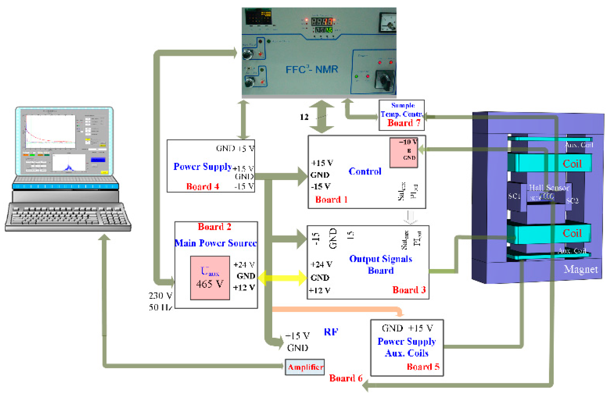
This type of equipment includes a set of subsystems as typically represented in Figure 1 [3]. In this equipment, the magnet [4] and the main power supply [5,6] are the core elements.
In recent years, small compact FFC NMR magnets using ferromagnetic cores have been developed [2,7]. These new types of magnets have much higher inductance than air core magnets [4,8] and require much lower currents to produce equivalent magnetic fields. However, the transitions between current levels (i.e., between magnetic field levels) require higher voltages. In general, the magnet design is optimized, having as main target the homogeneity of the magnetic flux density. The use of iron core magnets in FFC NMR also require a suitable control of the magnets’ hysteresis compensation and constitute an additional challenge in the development of ferromagnetic-core-based FFC NMR equipment [9].
Since the early days, the development of the FFC NMR power supplies has been a continuous challenge concerning their performance and modularity. One of the main challenges for the development of small low power FFC MNR equipment is the necessary compromise between the value of the working current, the current’s slew rate, and the voltages values applied to the semiconductors of the power supply. The present solution constitutes a progress for the FFC technique due to its low power consumption with linear control of the magnetic flux density, high efficiency, low maintenance, low volume and portability.
In this work, a solution is presented based on a power supply with low power consumption, portability, and low cost. This power supply, when connected to an optimized iron core magnet [9,10], present unique features, as for instance, a low-cost air cooling system, low operation noise, and sample alignment control system. Portability being an added value, this solution opens the possibility of using the FFC NMR technique for new users. Since, until now, this technique has been owned by research groups, this prototype can contribute to diversify the use of FFC relaxometry, mainly by technicians in industrial laboratories.
In this work, as a new approach, the power supply of the magnet is specifically designed to control directly the magnetic flux density cycles as required by the FFC application. FFC power supplies reported in literature use feedback control current and air-cored magnets [10,11,12,13]. They consider the system with a linear magnetic characteristic. For other hand, as referred before, iron-core magnets, due to its intrinsic nonlinear magnetic characteristic, require featuring the control loop with increased complexity, i.e., a direct control of the magnetic flux density, as described in this paper. This approach, albeit limited by the maximum magnetic flux density that can be measured (typically 25 mT), leads to incomparable benefits in terms of power consumption and demanded current: 6 times less than [12]; 15 times less than [11]; 10 times less than [10]; and 20 times less than [13].
With a Hall effect, sensor measuring directly the magnetic flux density in the sample room, the control loop is able to compensate disturbances in the magnetic flux density distributions, and all the drawbacks of an iron-core magnet can be overcome, as it is done with the proposed solution [9].
The new trends concerning the FFC NMR relaxometers are directly related with their applications. Considering, for instance, the food, materials development, or oil industries, desktop NMR relaxometer solutions are welcome as they might contribute to quality control processes and product development. On the other hand, medicine applications may require the development of equipment for human-size bodies. An example of a recent application is the “detection of osteoarthritis in knee and hip joints” [14] and the “measurement of fibrin concentration” [15]. Related with the food industry, relaxometric studies for food characterization were recently performed [16], as for instance “the case of balsamic and traditional balsamic vinegars” [17] and “water molecular dynamics during bread staling” [18]. In the pharmaceutical field, a recent example are the studies of “solubility and dissolution rate of poorly soluble drugs” [19].
This paper is organized as follows: Section 2 presents the characteristics of the main power supply and describes their operating modes; in Section 3, the control principles, the control command chains, and parameters are presented; in Section 4, experimental results illustrating the operation of the developed solutions under the FFC requirements are shown; in Section 5 conclusions are presented.
2. Power Supply
The power supply has a modular design based on boards built in-house with the following functionalities:
- Control circuit (Board 1);
- Main power source (nominal voltage: 24 V; nominal current: 5 A) and the auxiliary power supply (maximum voltage: 400 V) (Board 2);
- Decision control that generates the command signals of the main power supply and the auxiliary power supply (Board 3);
- Power supply of the electronic circuits (outputs: +15 V/0 V/−15 V; 0 V/+5 V) (Board 4);
- Power supply of the auxiliary coils, which compensate the Earth and parasitic magnetic fields (Board 5);
- Radio frequency circuit (excitation of the sample) (Board 6);
- Sample temperature controller (Board 7).
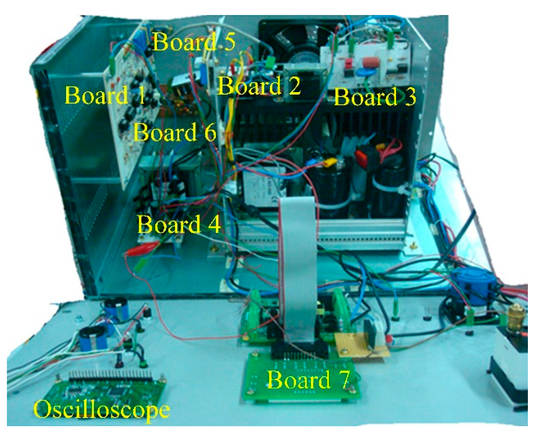
Conversely, to others, this FFC relaxometer [10,11,12], in addition to the circuits referred above, includes a Hall effect sensor that is placed inside the magnet, in the same section of the sample holder, i.e., the magnetic poles. The output of the Hall sensor is connected to the control system allowing for a direct control of the magnetic flux density. In Figure 2, a picture of the boards inside of the power supply housing is shown.
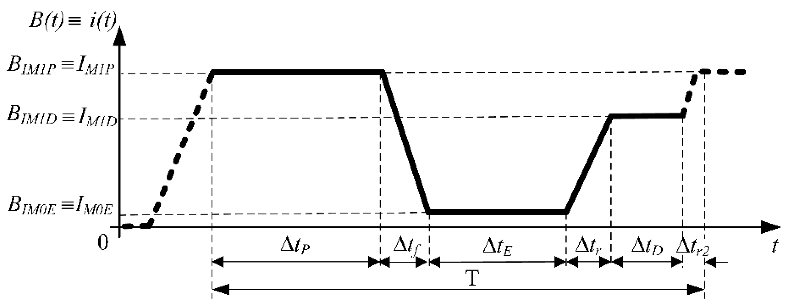
The main objective of FFC NMR power supplies is to control the magnetic flux density in order to perform generalized cycles, as represented in Figure 3 [1,3,6].
For this generalized magnetic flux density cycle, three levels are defined:
- BIM1P—magnetic flux density polarization;
- BIM0E—magnetic flux density evolution;
- BIM1D—magnetic flux density detection.
The transitions times from to ()—rise, and from to ()—fall, must be less than the values of the magnetization’s decay constant—spin-lattice relaxation rate, —for the sample studied but not so small that off-axis magnetic components appear and produce an irreversible loss of magnetization (adiabatic transition condition) [1]. In order to repeat the cycle, after the magnetic flux density changes to being the duration of this transition [1,3,6]. In an FFC NMR relaxometer, , consequently .
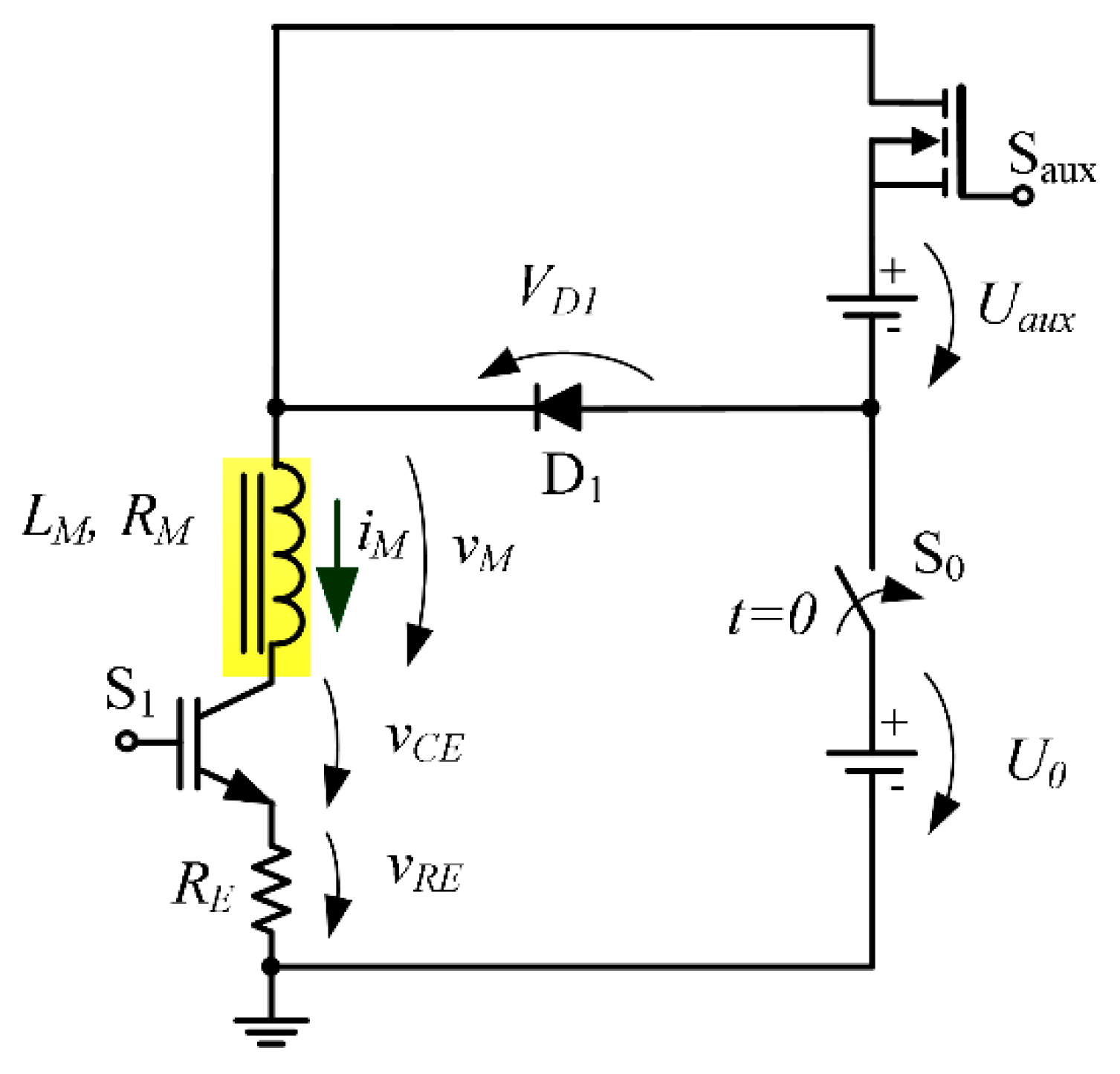
In Figure 4, the topology of power circuit is presented. The main elements are: A power semiconductor, , insulated gate bipolar transistor (IGBT type) together with an emitter resistor, , a low voltage source, , an auxiliary power supply, , a switch, , metal oxide semiconductor field-effect transistor (MOSFET type), a diode, , and the magnet characterized by its inductance and resistance, , , respectively. The switch, , corresponds to a general switch.
The operation conditions for this circuit require the following operation modes:
- “Steady-state” during times ,, and ;
- “Up” transition during time ; ;
- “Down” transition during time .
Framing the FFC requirements, the operation modes “Up” and “Down” need to be analyzed in order to validate the proposed solution.
- “Up” transition
A transition from the low () to a high magnetic flux density level ( or ), can be performed using only the main power source or with both main and auxiliary power supplies.
- Using only the main power source
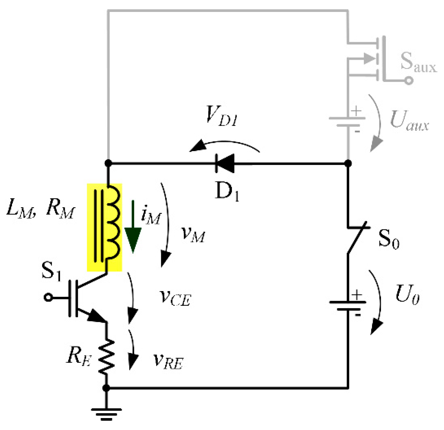
During the “Up” transition, the power circuit can be represented by an electrical equivalent circuit, presented in Figure 5, which is based on a single IGBT power semiconductor.
In the circuit of Figure 5, the magnet current is governed by the following equation:
where the diode voltage drop, the saturation IGBT collector-emitter voltage (), and the total resistance .
The natural time constant is given by
In spite of the fact that is sufficient to produce final target current , this level is achieved for times . For most FFC magnets is usually much larger than the values of therefore the use of the main current supply is not enough to fulfill the FFC NMR technique requirements. An auxiliary power source becomes necessary since the main power supply is designed to fulfill the operation of the system in steady-state.
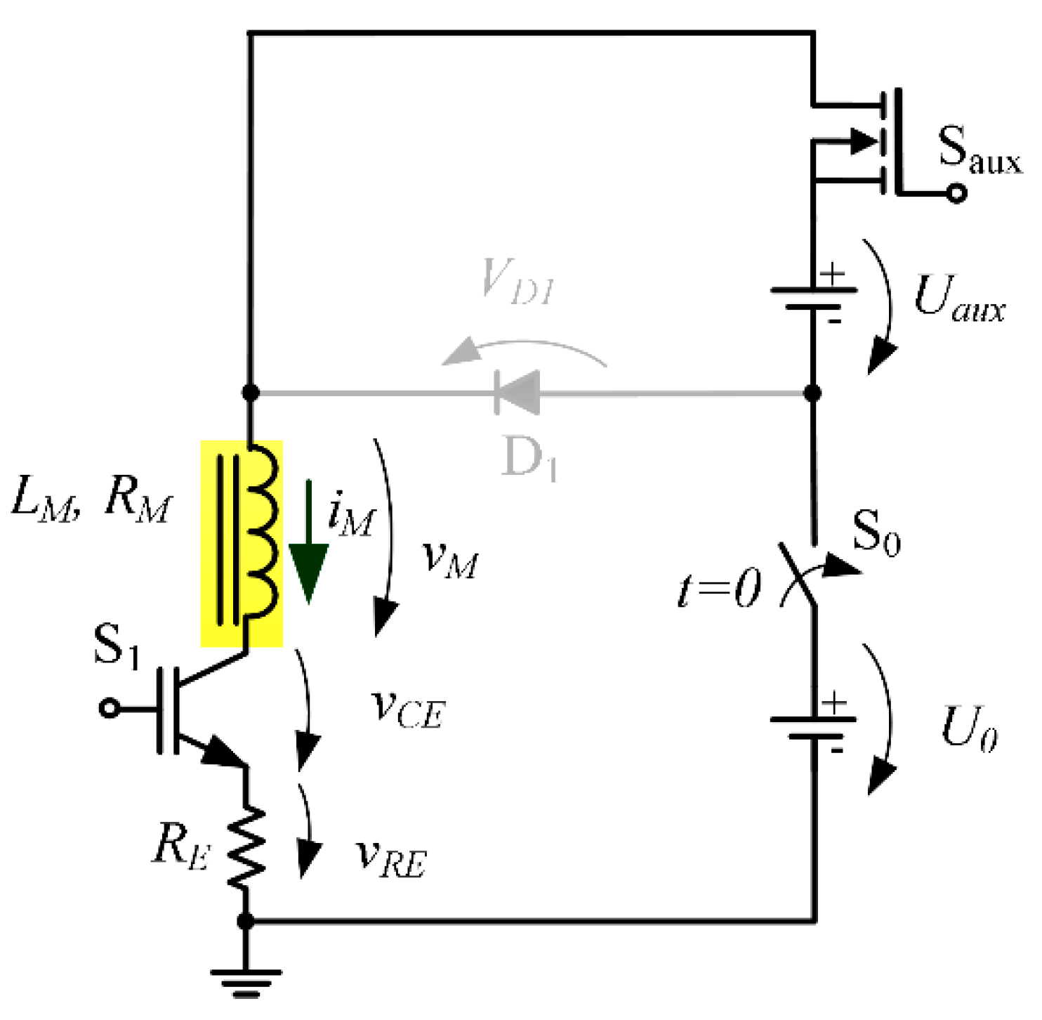
- With the auxiliary power supply
The electrical equivalent circuit including the auxiliary power supply during an “Up” transition is presented in Figure 6.
To perform an “Up” transition the switch is switched ON and the supply voltage is the sum of Under these conditions is OFF ().
For Figure 6, neglecting the drop voltage across , the magnet current is governed by:
From Equation (3), neglecting the resistive voltage drop the current rise rate is established by:
Despite the circuit natural time constant is maintained, one can increase the current rise rate by adjusting the auxiliary supply voltage (), so that can be reached after time , in order to fulfill the dynamic requirements of the application.
- B.
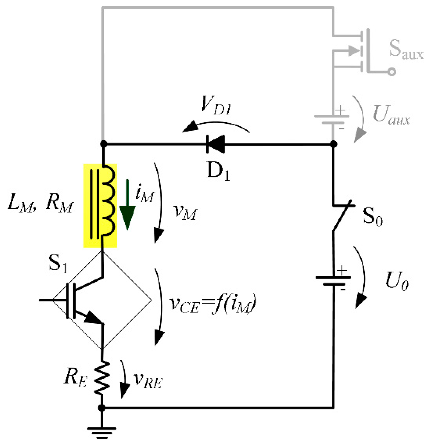
- “Down” transition
The transition from the high ( or ) to a low magnetic flux density level (), is performed taking advantage of the collector-emitter voltage drop of the IGBT semiconductor. The voltage in the active region of this semiconductor can be expressed by [20,21]:
where is a fictitious resistance relating the voltage with the current , and is a minimum value of that assures safe operation of the IGBT.
The electrical equivalent circuit during a “Down” transition is represented in Figure 7.
Merging Equation (1) with Equation (5) (neglecting ), under “Down” transition, the electrical circuit is governed by Equation (6)
and the current dynamics can be expressed by Equation (7)
where IM1P is the magnet current corresponding to the magnetic flux density level .
3. Control System
Conversely to the usual operation of the IGBT in Power Electronics, in this case, the linear operating zone is used in order to avoid switching ripples on the circuit. These would be adverse to NMR measurements.
Considering that the magnetic has linear characteristics, it can be assumed that the magnetic flux density () is proportional to the current ():
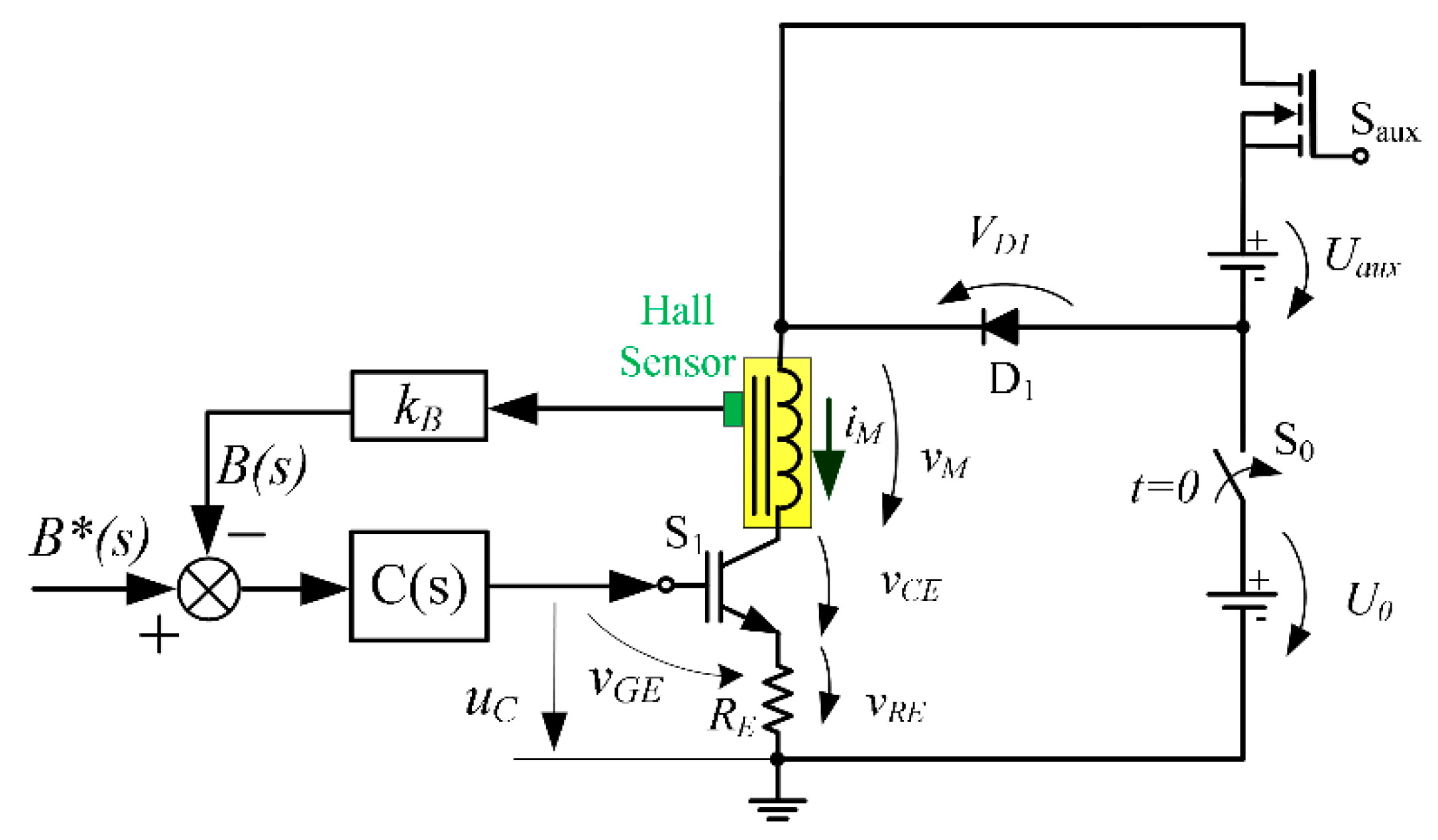
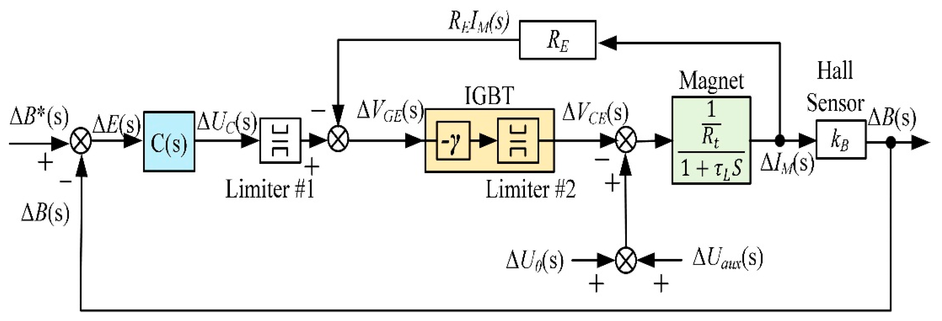
Since FFC technique requires an effective control of the magnetic flux density, it is advantageous to implement a control system based on a Hall effect sensor (Honeywell—SS94A2D) [22], as represented in Figure 8. This sensor has a sensitivity of 1.00 ± 0.02 mV/gauss and a linear behavior in the range [−2500, 2500] G, and presents an accuracy of 1:5000 fulfilling the FFC requirements.
In Figure 8, C(s) represents the controller’s transfer function and the gain of the Hall effect sensor. The gate–emitter voltage () is used to adjust the collector–emitter voltage () of the IGBT (S1) and consequently control the magnet current ().
In Figure 9, an incremental model of the circuit is presented. It is used to choose the type of controller, to set its parameters and to evaluate its performance.
In the incremental model, () can be set in line with the magnet block:
is the number of turns of the magnet, is the air gap cross-section of the magnetic core and is the magnetic reluctance.
The incremental model includes two limiters: “Limiter #1” limits the command voltage (), i.e., limits indirectly the magnet voltage; “Limiter #2” defines the collector–emitter saturation voltage of the IGBT ().
In the incremental study, it is assumed a linear relationship between the collector–emitter voltage () and the gate–emitter voltage (), given by the equation [20,21]:
The gate–emitter voltage depends on the control voltage, provided by the controller, and the voltage drop, as expressed by the following equation:
- Operating modes
- “Up” transition )
The “Up” transition occurs when a step-up signal in the reference level input () is imposed. The IGBT is saturated and a supply voltage () is applied to the magnet coils. The dynamic behavior of the magnetic flux density (and also the magnet current) during the “Up” transition depends on the load parameters , and , increasing the magnetic flux density according to the equation:
During , this transition is approximately linear, with the following behavior:
- “Down” transition ()
The reference signal during the “Down” transition ) is a downward ramp:
being the absolute value of the decreasing rate for the less favorable cases.
When the lower reference value of the magnetic flux density () is reached, the ramp is quenched.
The controller should act to increase the voltage , and, through this, to decrease the magnet current. For a good performance of the FFC-NMR system during , it is important that the output follow the reference, as closed as possible, i.e., decreasing the velocity error as much as possible.
The performances required during and are similar. However, due to the very fast drop of the magnetic flux density during , overshoots can occur affecting the settling time for this transient. In this case, a control with derivative action might be necessary. As stated in Section 2, the values and must be much smaller than the relaxation time T1 but not so small that transition induced spurious off-axis magnetic field components destroy the magnetic field alignment. The error tracking between the reference signal and the probed magnetic field signal is less critical during the magnetic field transitions than in the steady states.
- High magnetic flux density—steady-state (, , )
In steady state within time intervals and , the magnetic flux density remains constant at the levels and , respectively. The controller acts to adjust the magnet current in order to keep the magnetic flux density at the set value. When changing from the “Up” mode to the steady-state mode, the extinction of voltage is seen by the control chain as a disturbance, which is adequately compensated.
During these time intervals ( and ) it is essential that the controller includes an integral action to eliminate the static error and to compensate disturbances.
- Low magnetic flux density—steady-state ()
During the time interval the magnetic flux density remains constant at its minimum value .
- B.
- Parameters of the Controller
According to the operation modes described above, the type of controller is clearly framed by the required dynamic behavior during the “Down” transition. The controller should be properly set to ensure both a null static error and to avoid overshoot. To fulfill these requirements a classic proportional–integral (PI) controller is used. This controller can have an analog implementation [21] or a digital solution based on a microcontroller [23]. The approach above is based on the analog implementation.
The downward ramp reference signal () must have a very short time (typically, is 3 ms) and the input signal, as first approach, can be approximated to a step “Down.” Thus, the system can be controlled using a PI controller designed for optimum response to step inputs. This approach requires further validation based on the static and velocity errors.
The optimal response of second order systems, according to the ITAE (integral of the time weighted absolute error) criteria, for a step input is represented by the transfer function:
The transfer function representing the PI controller is:
where:
Introducing the transfer function of the controller C(s) in Figure 9, the incremental block diagram can be simplified, as represented in Figure 10.
In Figure 10, the simplified block corresponding to the power circuit is represented by a static gain A and the time constant :
The resistor is useful to implement an indirect feedback control of the magnet current as represented in Figure 9. This resistance influences and allows to decrease the time constant , and therefore, contributes to decrease the global gain of the control chain.
The closed loop transfer function () of the simplified block diagram is given by Equation (21)
where it is assumed that:
This allows neglecting the influence of the zero in the following synthesis of the PI controller. Looking for the optimal response to a step input, the equality of Equations (15) and (21) leads to:
From Equation (24) it is obtained that:
or
Obtaining k from Equation (26), the following condition needs to be verified, i.e., it is a solution of a 2nd order equation with real roots and positive discriminant:
Fulfilling the inequality Equation (27) leads to the following relationship between and L:
Thus, the condition expressed by Equation (22) is satisfied leading to a real value for the gain . Introducing the relation Equation (22) in Equation (26), the gain values corresponding to the considered integer n are obtained.
Replacing Equation (20) and Equation (21) in Equation (30), the integral gain can be calculated using the following equation:
Using Equation (18), the proportional gain is:
Considering n = 10 and using the smallest gain value obtained from Equation (29), results in and .
4. Experimental Results and Analysis
The validation of the proposed solution is achieved by performing “Up” and “Down” transitions between different magnetic flux density levels with the system parameters summarized in Table 1. In the following, several transitions of the magnetic flux density (measured getting the analog signal from the Hall effect sensor) and the behavior of the collector–emitter voltage and the magnet current are analyzed.
As expected, when is disabled, the transient lasts near 150 ms, which is too high for a generalized use of the FFC NMR technique. So, it is the use of an auxiliary power supply () during the “Up” transition, which permits to achieve the magnetic flux density rise time requirements.
- Magnetic flux density—“Up” and “Down” transition
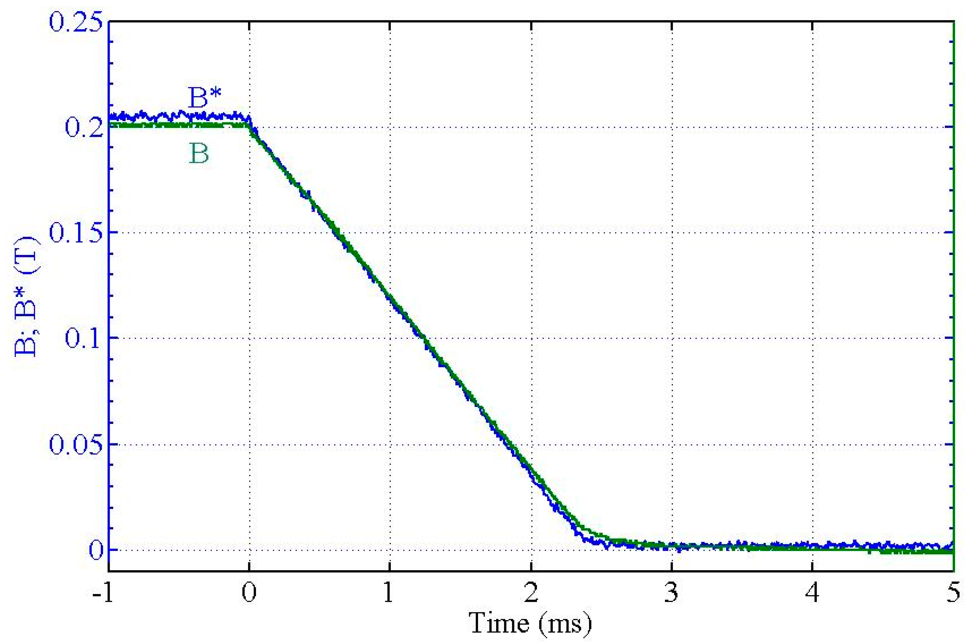
In Figure 11 is shown the dynamic behavior of the magnetic flux density during an “Up” transition using . The magnetic flux density reference is denoted by (. In Figure 12 is shown the dynamic behavior of the magnetic flux density during a “Down” transition.
Setting (Figure 11), the switching time between the minimum and maximum magnetic flux density levels lasts less than 3 ms which is within the expected limits.
From Figure 12, “Down” transition, it can be seen that the magnet flux density follows its reference very closed, fulfilling the FFC NMR requirements.
- B.
- Collector–emitter voltage
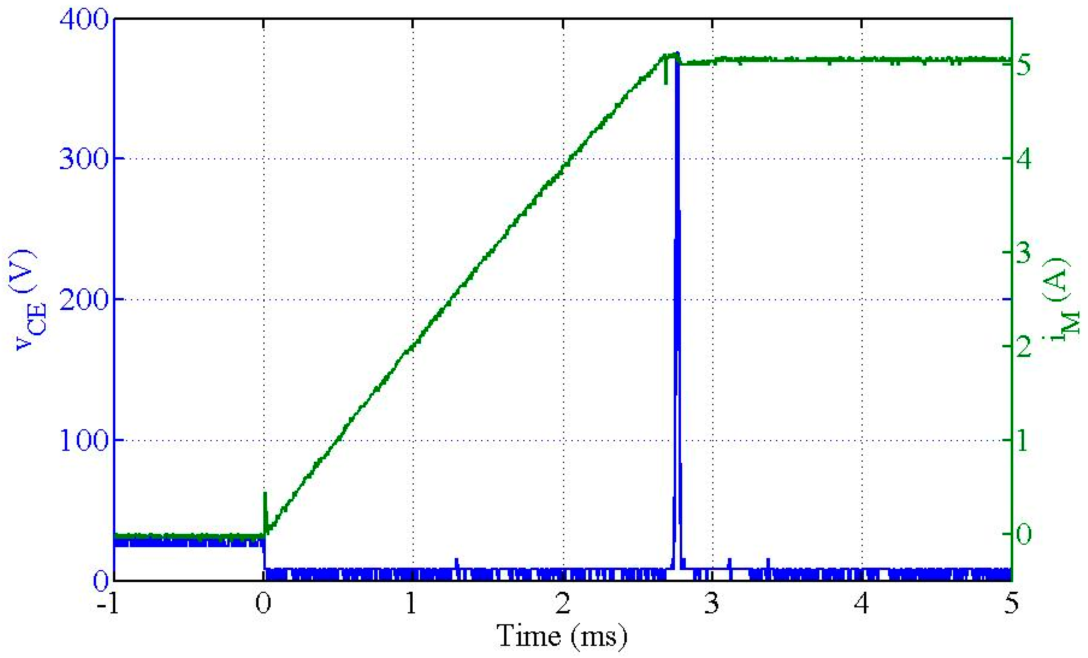
Figure 13 presents the experimental results of the collector–emitter voltage of the IGBT and magnet current during “Up” transitions.
For the “Up” transition, the initial voltage of the collector–emitter voltage () corresponds to the voltage of the power source . During the transition, drops to the saturation value of the IGBT (), remaining at this voltage until reaching the target magnetic flux density level. At the instant that the magnetic flux density reaches the upper level, it is observed a collector–emitter voltage peak around 380 V. This results of a delay on the auxiliary switch (Saux) turn off, resulting on a delay of its control system. The consequence of this peak is a current variation of about 0.11 A (current change from 5.11 A to 5.00 A) in about 0.08 ms.
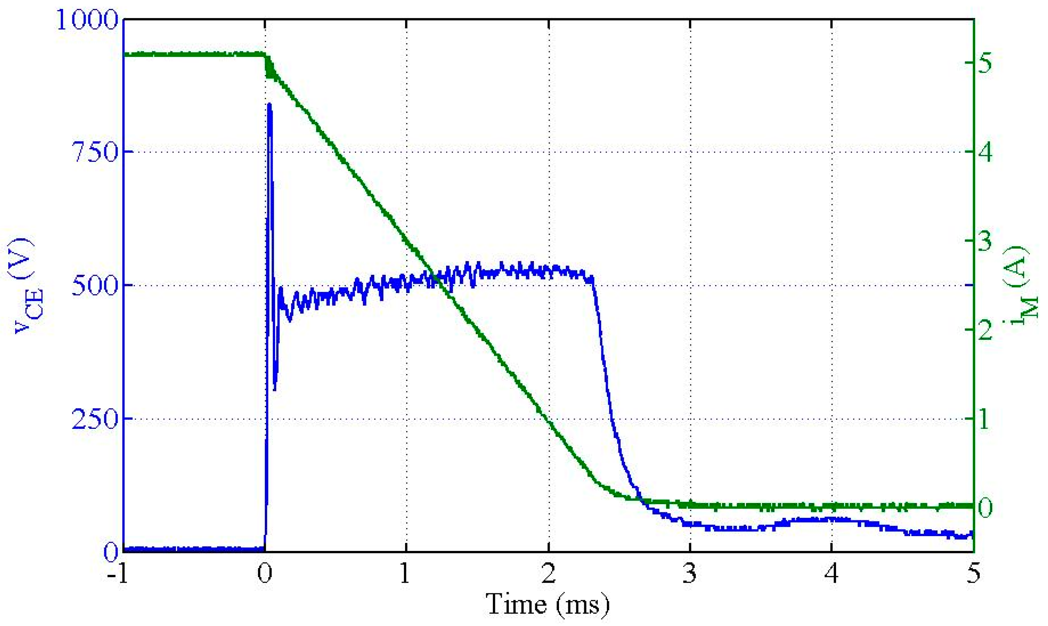
Figure 14 presents the experimental results of the collector–emitter voltage of the IGBT during “Down” transition.
For the “Down” transition (Figure 14), at the initial instant it is observed a peak of about 840 V with a high damping oscillatory characteristic that is due to the response of the controller. This transient is not visible on the controllable variable, the magnetic flux density or in the magnet current, but it is visible on its derivative that is, on the magnet and voltages. It is due to the zero on the closed loop transfer function Equation (21) that was neglected in the synthesis of the PI controllers. After the peak, the voltage steadies around a value established by the electromotive force generated in the magnet due to decreasing current. When the current reaches the lowest level, in this case close to zero, the voltage is within the range of the main power source voltage .
- C.
- Command voltages
Analyzing the previous results of the “Up” transitions of the magnetic flux density, it can be concluded that it develops according to the requirements of the FFC-NMR purpose. It is important to note a minimum magnetic flux density overshoot, which is the major requisite for this application. Additionally, for the “Down” transition, the observed dynamics are within the limits imposed by the FFC-NMR measurement conditions [1,3,6]. These results are directly related with the control circuit and the command voltages of the control chain.
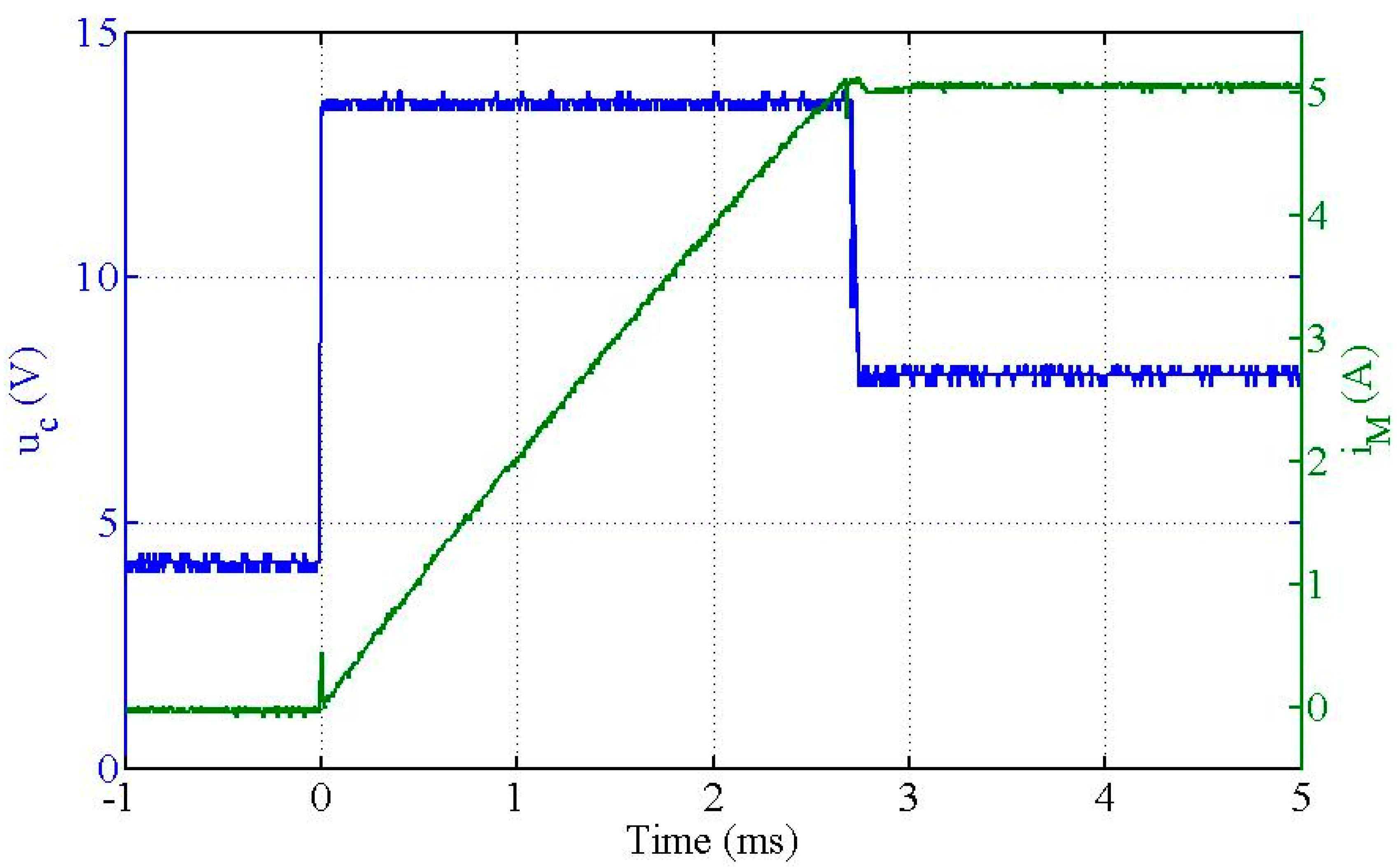
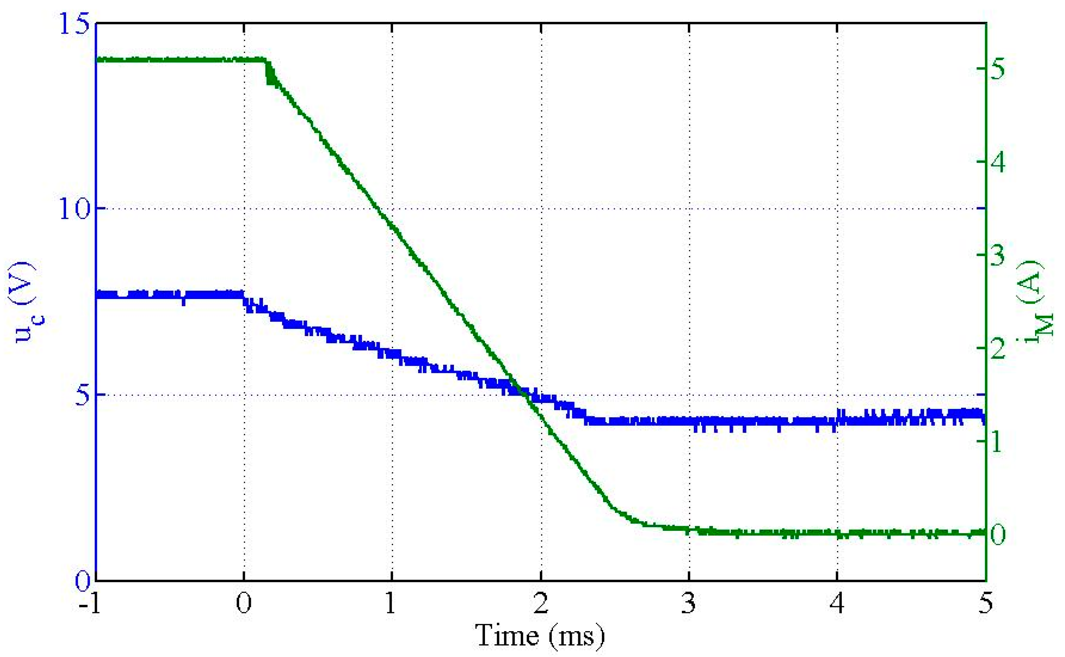
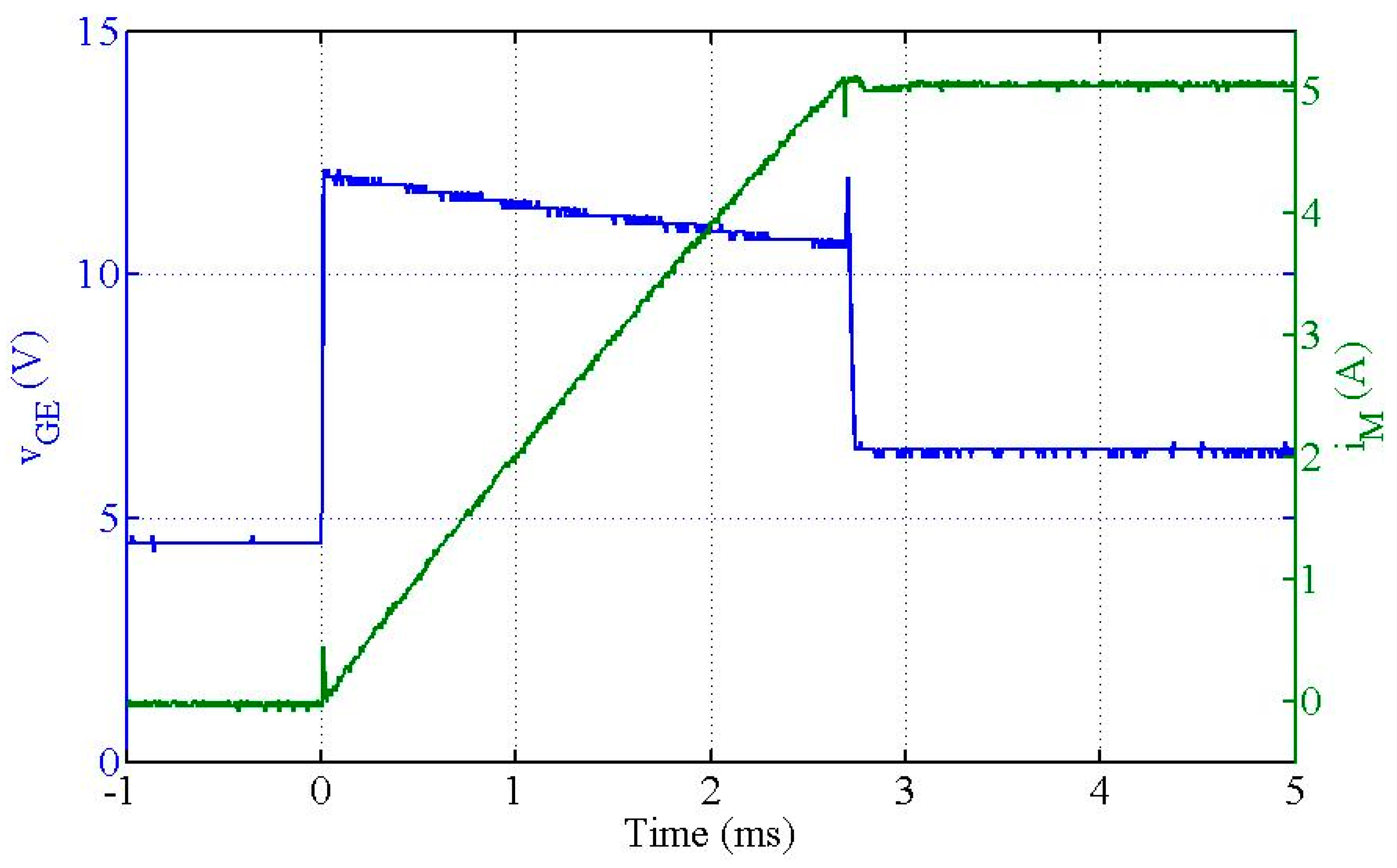
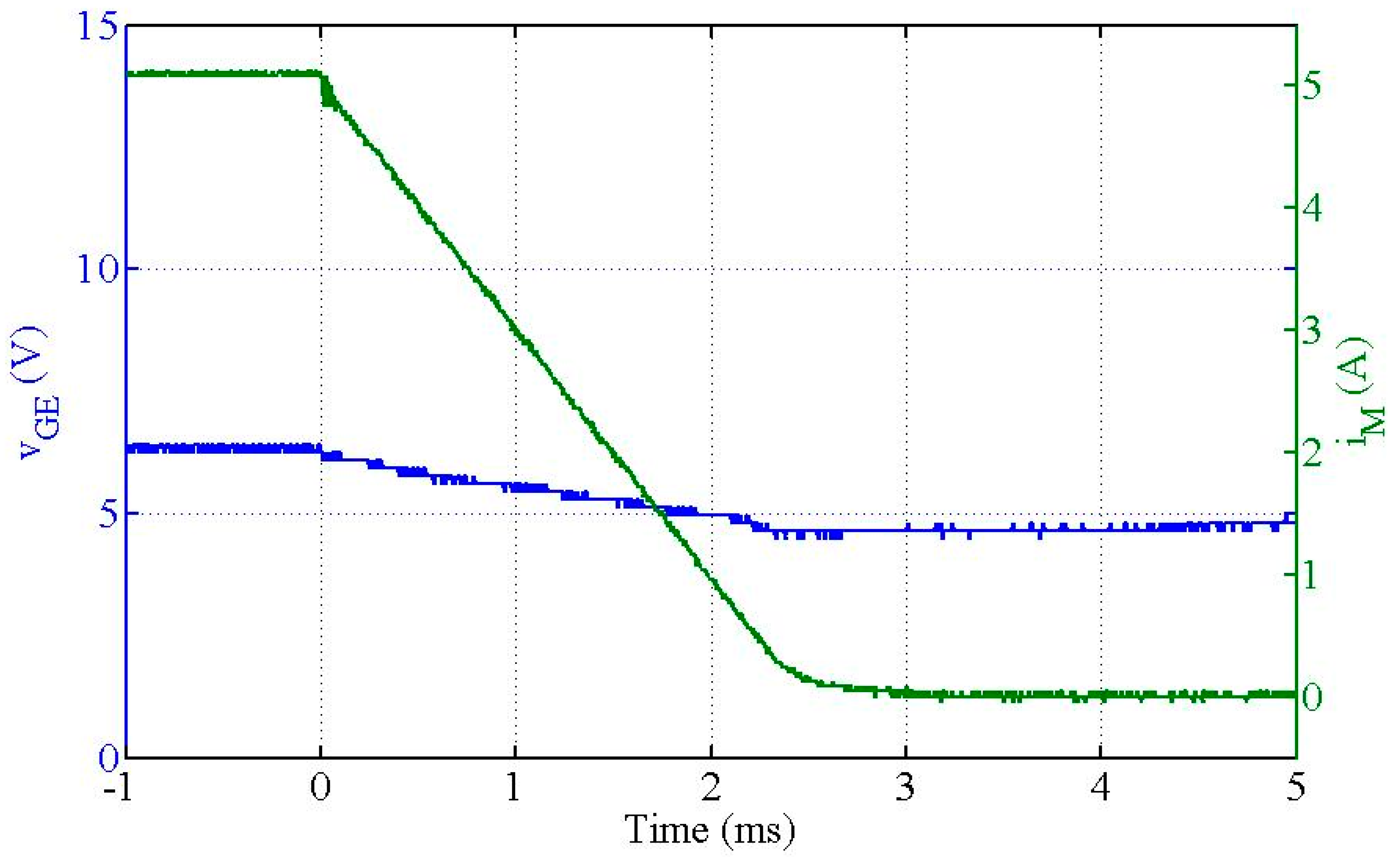
Figure 15, Figure 16, Figure 17 and Figure 18 show the experimental results of the command voltage uc and the gate–emitter voltage (VGE) of the IGBT during “Up” and “Down” transitions, respectively.
The results shown in these figures are according to the specifications described above.
- D.
- Experimental magnetization
The power source was successfully used to operate a FFC NMR relaxometer and to perform spin-lattice relaxation measurements for the liquid crystal 5CB commonly used to test the performance of FFC equipment.
In order to obtain the time evolution of the magnetization, it is necessary to obtain the free induction decay (FID) and estimate its initial value.
The digital radio frequency quadrature detection system outputs the real, imaginary parts, and also the absolute value of the FID [13,24].
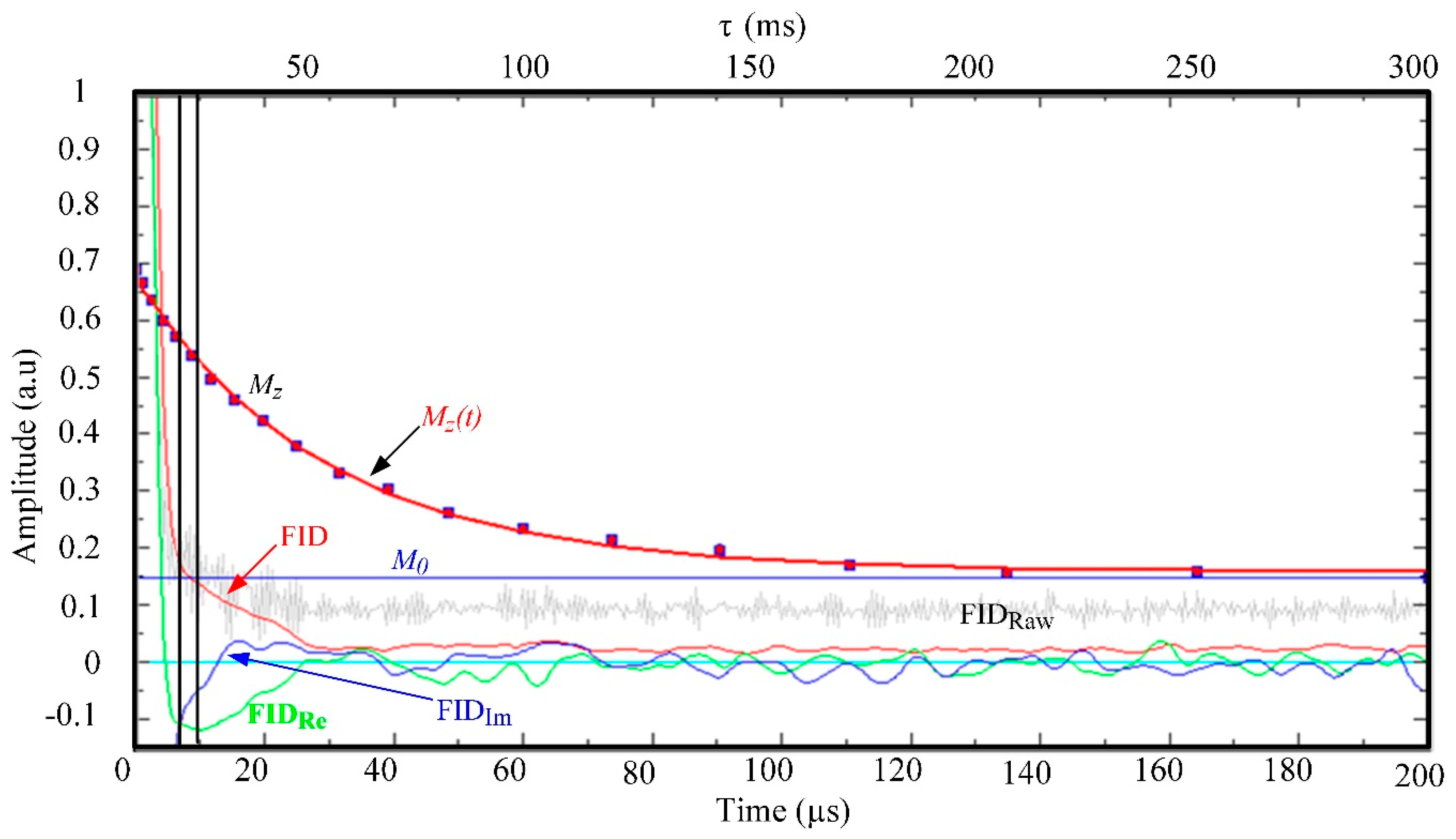
Due to the relatively poor signal-to-noise ratio and presence of high-frequency noise, some degree of noise elimination is required before obtaining the absolute value, otherwise the absolute value will have a positive offset. In Figure 19 are shown typical raw free induction decay signal (FIDraw), and the noise filtered signals: FIDRe, real part; FIDIm, imaginary part; and FID. It should be referred that the system is assembled in order to guarantee electromagnetic compatibility (EMC) among all the parts.
During a magnetic field cycle, the FID signal is collected after the evolution time τ and the magnetization can be estimated from the initial value of FID. The vertical lines in Figure 19 define a time window typically used to obtain an average value of the FID’s initial value. In Figure 19 is shown the magnetization evolution for the chemical compound 5CB at 300 kHz@299 K. Each point was obtained for a different evolution time τ using the same time average window of FID.
The experimental values , can be fitted by the theoretical equation:
obtained from the Bloch equations [1]. The fitting curve can also be seen in Figure 19 together with the curve corresponding to the asymptotic value of the magnetization .
These results clearly confirm that described power supply fulfils the FFC requirements and can be used to operate an NMR spectrometer.
5. Conclusions
The core aspects of a main power source for an FFC NMR relaxometer are described and discussed in this paper. The implemented solution was designed specifically to directly control the magnetic flux density in the sample’s holder using a Hall sensor. This solution constitutes an advance in the development of FFC-NMR solutions since any disturbance or nonlinearity in the magnetic flux density distribution is compensated.
Under standard operation conditions, it is exemplified the dynamic behavior of the magnetic flux density during a typical FFC experiment. As it can be observed using the experimental results shown, the magnetic flux density transients are accurate and fast fulfilling the specifications of an FFC NMR measurement of magnetization decay for low magnetic fields.
A linear relationship between the magnetic flux density and the magnet current made it possible to implement different control strategies, for “Up” and “Down” field transitions, and steady states.
Author Contributions
The following statements should be used “conceptualization, A.R., D.M.S., P.S., E.M. and G.M.; methodology, A.R., D.M.S., P.S.; software, A.R., D.M.S., P.S.; validation, A.R., D.M.S., P.S., E.M. and G.M.; formal analysis, A.R., D.M.S., P.S., E.M. and G.M.; investigation, A.R., D.M.S., P.S., E.M. and G.M.; resources, A.R., D.M.S., P.S., E.M. and G.M.; data curation, A.R., D.M.S., P.S.; writing—original draft preparation, A.R., D.M.S., P.S., E.M. and G.M.; writing—review and editing, A.R., D.M.S., P.S.; visualization, A.R., D.M.S., P.S.; supervision, D.M.S., P.S., E.M. and G.M.; project administration, A.R., P.S.; funding acquisition, A.R., P.S..”
Acknowledgments
This work was supported by national funds through Instituto Politécnico de Setúbal, ISEL/Instituto Politécnico de Lisboa, Fundação para a Ciência e a Tecnologia (FCT) with reference UID/CEC/50021/2019 and UID/CTM/04540/2019.
Conflicts of Interest
The authors declare no conflicts of interest.
References
- Noack, F. NMR Field-Cycling Spectroscopy: Principles and Applications. Prog. NMR Spectrosc. 1986, 18, 171–276. [Google Scholar] [CrossRef]
- Fujara, F.; Kruk, F.; Privalov, A. Solid State Field-Cycling NMR Relaxometry: Instrumental Improvements and New Applications. Prog. Nucl. Magn. Reson. Spectrosc. 2014, 89, 39–69. [Google Scholar] [CrossRef] [PubMed]
- Anoardo, E.; Galli, G.; Ferrante, G. Fast-Field-Cycling NMR: Applications and Instrumentation. Appl. Magn. Reson. 2001, 20, 365–404. [Google Scholar] [CrossRef]
- Lips, O.; Privalov, A.; Dvinskikh, S.; Fujara, F. Magnet Design with High B0 Homogeneity for Fast-Field-Cycling NMR Applications. J. Magn. Reson. 2001, 149, 22–28. [Google Scholar] [CrossRef] [PubMed]
- Seitter, R.; Kimmich, R. Magnetic Resonance: Relaxometers. In Encyclopedia of Spectroscopy and Spectrometry; Academic Press: London, UK, 1999; pp. 2000–2008. [Google Scholar]
- Kimmich, R.; Anoardo, E. Field-Cycling NMR relaxometry. Prog. NMR Spectrosc. 2004, 44, 257–320. [Google Scholar] [CrossRef]
- Sousa, D.M.; Marques, G.D.; Cascais, J.M.; Sebastião, P. Desktop Fast-Field Cycling Nuclear Magnetic Resonance Relaxometer. Solid State Nucl. Magn. Reson. 2010, 38, 36–43. [Google Scholar] [CrossRef] [PubMed]
- Kim, S.; Fukada, S.; Nomura, R.; Ueda, H. Development of HTS Bulk NMR Relaxometry with Ring-shaped Iron. IEEE Trans. Appl. Supercond. 2017, 28, 1–5. [Google Scholar] [CrossRef]
- Roque, A.; Sousa, D.; Margato, E.; Machado, V.; Sebastião, P.; Marques, G. Magnetic Flux Density Distribution 3D Analysis in the Air Gap of a Ferromagnetic Core with Superconducting Blocks. IEEE Trans. Appl. Supercond. 2015, 25. [Google Scholar] [CrossRef]
- Constantin, J.; Zajicek, J.; Brown, F. Fast Field-Cycling Nuclear Magnetic Resonance Spectrometer. Rev. Sci. Instrum. 1996, 67, 2113–2122. [Google Scholar]
- Rommel, E.; Mischker, K.; Osswald, G.; Schweikert, K.; Noack, F. A powerful NMR field-cycling device using GTO’s and MOSFET’s for relaxation dispersion and zero-field studies. J. Magn. Reson. 1986, 70, 219–234. [Google Scholar]
- Sousa, D.; Fernandes, P.; Marques, G.D.; Ribeiro, A.C.; Sebastião, P. Novel Pulsed Switched Power Supply for a Fast Field Cycling NMR Spectrometer. Solid State Nucl. Magn. Reson. 2004, 25, 160–166. [Google Scholar] [CrossRef] [PubMed]
- Products—Stelar. Available online: http://www.stelar.it/products.htm (accessed on 1 February 2018).
- Broche, L.M.; Ashcrof, G.P.; Lurie, D.J. Detection of osteoarthritis in knee and hip joints by fast field-cycling NMR. Magn. Reson. Med. 2012, 68, 358–362. [Google Scholar] [CrossRef] [PubMed]
- Broche, L.M.; Ismail, S.R.; Booth, N.A.; Lurie, D.J. Measurement of fibrin concentration by fast field-cycling NMR. Magn. Reson. Med. 2012, 67, 1453–1457. [Google Scholar] [CrossRef] [PubMed]
- Kirtil, E.; Oztop, M. 1H Nuclear Magnetic Resonance Relaxometry and Magnetic Resonance Imaging and Applications in Food Science and Processing. Food Eng. Rev. 2016, 8, 1–22. [Google Scholar] [CrossRef]
- Baroni, S.; Consonni, R.; Ferrante, G.; Aime, S. Relaxometric studies for food characterization: The case of balsamic and traditional balsamic vinegars. J. Agric. Food Chem. 2009, 57, 3028–3032. [Google Scholar] [CrossRef] [PubMed]
- Curti, E.; Bubici, S.; Carini, E.; Baroni, S.; Vittadini, E. Water molecular dynamics during bread staling by Nuclear Magnetic Resonance. LWT-Food Sci. Technol. 2011, 44, 854–859. [Google Scholar] [CrossRef]
- Paudel, A.; Geppi, M.; Mooter, G. Structural and Dynamic Properties of Amorphous Solid Dispersions: The Role of Solid-State Nuclear Magnetic Resonance Spectroscopy and Relaxometry. J. Pharm. Sci. 2014, 103, 2635–2662. [Google Scholar] [CrossRef] [PubMed]
- Sousa, D.; Rommel, E.; Santana, J.; Silva, F.; Sebastião, P.; Ribeiro, A. Power Supply for a Fast Field Cycling NMR Spectrometer Using IGBTs Operating in the Active Zone. In Proceedings of the 7th European Conference on Power Electronics and Applications (EPE1997), Trondheim, Norway, 8–10 September 1997. [Google Scholar]
- Roque, A.; Maia, J.; Margato, E.; Sousa, D.; Marques, G. Control and dynamic behaviour of a FFC NMR power supply. In Proceedings of the IECON 2013—39th Annual Conference of the IEEE Industrial Electronics Society, Vienna, Austria, 10–13 November 2013; pp. 5945–5950. [Google Scholar]
- Sensing and Control Honeywell Inc. Hall Effect Linear Position Sensor SS94A2D; Sensitivity: 1.00 ± 0.02 mV/gauss; Linear Behavior in the Range [–2500,2500] G. Available online: http://pdf1.alldatasheet.com/datasheet-pdf/view/539500/HONEYWELL/SS94A2D.html (accessed on 1 March 2017).
- Lopes, R.; Sebastião, P.J.; Roque, A.; Sousa, D.M. Microcontroller of the Power Supply of a Fast Field Cycling Relaxometer. In Proceedings of the 19th International Conference on Industrial Technology, ICIT’18, Lyon, France, 20–22 February 2018. [Google Scholar]
- SpinCore Technologies, Inc. Available online: www.spincore.com (accessed on 15 March 2017).
Figure 1.
Set of circuits of a fast field cycling (FFC) nuclear magnetic resonance (NMR) relaxometer.
Figure 1.
Set of circuits of a fast field cycling (FFC) nuclear magnetic resonance (NMR) relaxometer.

Figure 2.
Inside view of the power supply housing.

Figure 3.
Generalized magnetic flux density and current cycles.

Figure 4.
Generic topology of the power supply.

Figure 5.
Equivalent circuit when performing an “Up” transition disabling the auxiliary power supply.
Figure 5.
Equivalent circuit when performing an “Up” transition disabling the auxiliary power supply.

Figure 6.
Equivalent circuit when performing an “Up” transition with the contribution of both main and auxiliary power supplies.
Figure 6.
Equivalent circuit when performing an “Up” transition with the contribution of both main and auxiliary power supplies.

Figure 7.
Equivalent circuit when performing a “Down” transition.

Figure 8.
Conceptual feedback control system coupled to the main current circuit.

Figure 9.
Block diagram of the incremental model. IGBT: Insulated gate bipolar transistor.

Figure 10.
Simplified block diagram of the incremental model.

Figure 11.
“Up” transition of the magnetic flux density between and .

Figure 12.
“Down” transition of the magnetic flux density between and .

Figure 13.
Collector–emitter voltage of the IGBT and magnet current during an “Up” transition between and .
Figure 13.
Collector–emitter voltage of the IGBT and magnet current during an “Up” transition between and .

Figure 14.
Collector–emitter voltage of the IGBT during a “Down” transition between and .

Figure 15.
Command voltage (uc) during an “Up” transition between and .

Figure 16.
Command voltage (uc) during a “Down” transition between and .

Figure 17.
Gate–emitter voltage of the IGBT during an “Up” transition between and .

Figure 18.
Gate–emitter voltage of the IGBT during a “Down” transition between and .

Figure 19.
Screen shot of the magnetization evolution during an FFC experiment. The raw free induction decay (FID) and filtered signals FID, FIDRe, and FIDIm are shown in gray, red, green, and blue lines. The vertical black lines define the time window where the FID is averaged to estimate the experimental . The process is repeated for different evolution times τ, as explained in the text. The fitting curve is also shown as explained in the text (color online).


Table 1.
Systems parameters.
| Parameters | Value | |
|---|---|---|
| RM | magnet resistor | 3 Ω |
| LM | magnet induction | 270 mH |
| RE | emitter resistor | 0.3 Ω |
| Uaux | auxiliary power supply | 500 V |
| U0 | source voltage | 24 V |
| KB | Hall effect sensor gain | 0.04 V/T |
| γ | gain (IGBT catalogue) | 700 |
| ΔtP | polarization time | 5–5000 ms |
| Δtf | switching “Down” time | ≤3 ms |
| ΔtE | evolution time | 5–5000 ms |
| Δtr | switching “Up” time | ≤3 ms |
| ΔtD | detection time | ≤100 µs |
| Δtr2 | switching “Up” time | ≤3 ms |
© 2019 by the authors. Licensee MDPI, Basel, Switzerland. This article is an open access article distributed under the terms and conditions of the Creative Commons Attribution (CC BY) license (http://creativecommons.org/licenses/by/4.0/).
Share and Cite
MDPI and ACS Style
Roque, A.; Sousa, D.M.; Sebastião, P.; Margato, E.; Marques, G. FFC NMR Relaxometer with Magnetic Flux Density Control. J. Low Power Electron. Appl. 2019, 9, 22. https://doi.org/10.3390/jlpea9030022
AMA Style
Roque A, Sousa DM, Sebastião P, Margato E, Marques G. FFC NMR Relaxometer with Magnetic Flux Density Control. Journal of Low Power Electronics and Applications. 2019; 9(3):22. https://doi.org/10.3390/jlpea9030022
Chicago/Turabian StyleRoque, António, Duarte M. Sousa, Pedro Sebastião, Elmano Margato, and Gil Marques. 2019. "FFC NMR Relaxometer with Magnetic Flux Density Control" Journal of Low Power Electronics and Applications 9, no. 3: 22. https://doi.org/10.3390/jlpea9030022
Note that from the first issue of 2016, this journal uses article numbers instead of page numbers. See further details here.