Article

Early Yield Prediction Using Image Analysis of Apple Fruit and Tree Canopy Features with Neural Networks

1
College of Information Science and Technology, Agricultural University of Hebei, Baoding 071001, China
2
Institute of Agricultural Engineering, Faculty of Agriculture, University of Bonn, 53115 Bonn, Germany
3
Key Lab of Agricultural Information Acquisition Technology, China Agricultural University, Beijing 100083, China
4
INRES-Horticultural Science, Faculty of Agriculture, University of Bonn, 53121 Bonn, Germany
*
Author to whom correspondence should be addressed.
J. Imaging 2017, 3(1), 6; https://doi.org/10.3390/jimaging3010006
Submission received: 30 September 2016 / Revised: 23 December 2016 / Accepted: 11 January 2017 / Published: 19 January 2017
(This article belongs to the Special Issue Image Processing in Agriculture and Forestry)

Abstract

:
(1) Background: Since early yield prediction is relevant for resource requirements of harvesting and marketing in the whole fruit industry, this paper presents a new approach of using image analysis and tree canopy features to predict early yield with artificial neural networks (ANN); (2) Methods: Two back propagation neural network (BPNN) models were developed for the early period after natural fruit drop in June and the ripening period, respectively. Within the same periods, images of apple cv. “Gala” trees were captured from an orchard near Bonn, Germany. Two sample sets were developed to train and test models; each set included 150 samples from the 2009 and 2010 growing season. For each sample (each canopy image), pixels were segmented into fruit, foliage, and background using image segmentation. The four features extracted from the data set for the canopy were: total cross-sectional area of fruits, fruit number, total cross-section area of small fruits, and cross-sectional area of foliage, and were used as inputs. With the actual weighted yield per tree as a target, BPNN was employed to learn their mutual relationship as a prerequisite to develop the prediction; (3) Results: For the developed BPNN model of the early period after June drop, correlation coefficients (R2) between the estimated and the actual weighted yield, mean forecast error (MFE), mean absolute percentage error (MAPE), and root mean square error (RMSE) were 0.81, −0.05, 10.7%, 2.34 kg/tree, respectively. For the model of the ripening period, these measures were 0.83, −0.03, 8.9%, 2.3 kg/tree, respectively. In 2011, the two previously developed models were used to predict apple yield. The RMSE and R2 values between the estimated and harvested apple yield were 2.6 kg/tree and 0.62 for the early period (small, green fruit) and improved near harvest (red, large fruit) to 2.5 kg/tree and 0.75 for a tree with ca. 18 kg yield per tree. For further method verification, the cv. “Pinova” apple trees were used as another variety in 2012 to develop the BPNN prediction model for the early period after June drop. The model was used in 2013, which gave similar results as those found with cv. “Gala”; (4) Conclusion: Overall, the results showed in this research that the proposed estimation models performed accurately using canopy and fruit features using image analysis algorithms.

1. Introduction

Early and accurate prediction of fruit yield is relevant for the market planning of the fruit industry, trade, supermarkets, as well as for growers and exporters to plan for the need of labour and bins, storage, packing materials, and cartons [1]. In the European Union (EU), about 12 million tons of apples are harvested every year, making it the most important fruit crop in the EU with year- to year variations of ca. two million tons. Yield prediction becomes essential after the last natural fruit abortion, i.e., June drop, when the first reliable yield estimates may be obtained and fruit are still small, green, and often occluded by leaves or other fruit, until harvest time; the accuracy of yield prediction and challenges change during fruit ontogeny. To date, yield prediction is mainly based on historic performance of an orchard in the previous years, i.e., empirical data. In order to improve the accuracy and efficiency for apple yield estimation, the automatic prediction using computer vision technology is increasingly receiving attention [2,3,4,5,6,7,8,9].
Previous apple detection studies concentrated on the late period of fruit maturation, when the number of fruits obtained from image analysis closely correlated between algorithm prediction and manually counted fruits in an image. Stajnko et al. [2] segmented cv. “Jonagold” apple fruit from the image taken on 7 September using colour features and surface texture. Fruit detection rates in the images were 89% of the apples visible on the images. Kelman and Linker [8] detected mature green apples in tree images using shape analysis and the correct detection of the apples was 85% of the apples visible in the images.
Moreover, to predict yield during the early growing period, Linker et al. [10] aimed to detect green “Golden Delicious” apple fruit from RGB images on only a part of an apple tree to facilitate the study; the algorithm accurately detected more than 85% of the apples visible in the images under natural illumination. Zhou et al. [5] proposed a recognition algorithm based on colour features to estimate the number of young “Gala” apples after June drop with a close correlation coefficient of R2 of 0.80 between apples detected by the fruit counting algorithm and those manually counted and R2 of 0.57 between apples detected by the fruit counting algorithm and actual harvested yield.
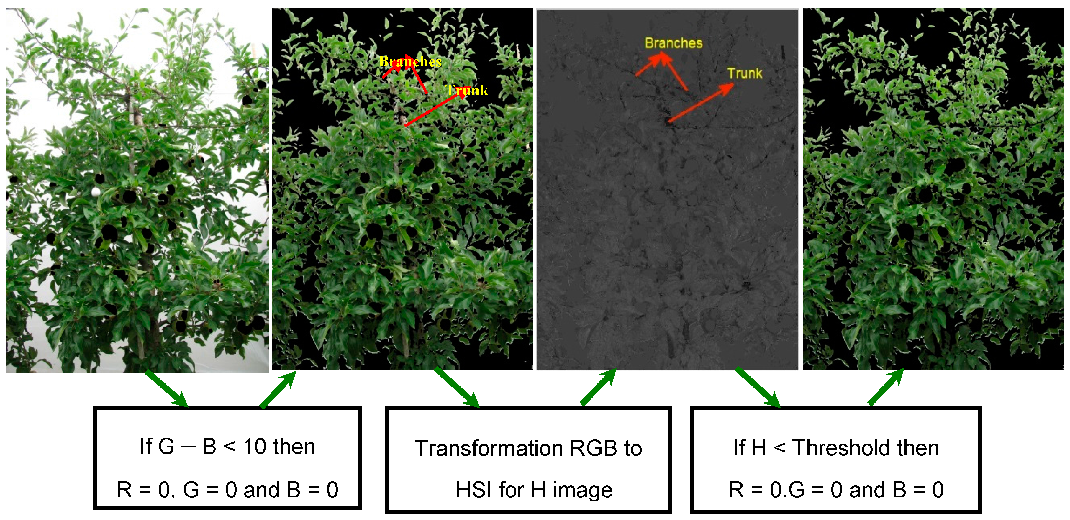
However, as noted in some of these studies, some regions of the apple tree are occluded, where leaves cover the apple fruit, making their assessment difficult during counting in the orchard. A certain number of fruit grow well inside the canopy close to the tree trunk, especially as trees grow older and into their high yielding phase, and pose a challenge to detect, especially, in the early stages of fruit growth. Hence, the present work is based on the hypothesis that these limitations with image processing to detect fruit early in the season may be overcome by the integration of characteristics of the canopy structure of the tree. From an apple tree canopy image, the features of the canopy structure are extracted by image processing [2,5]. There are artificial intelligence algorithms, which could be employed to model the relationship between the features and harvested yield.
An artificial neural network (ANN), as a commonly used machine learning algorithm, has the potential of solving such problems, when the relationship between the inputs and outputs is not well understood or is difficult to translate into a mathematical function. Many ANN applications dealing with this similar situation in agriculture have been reported [11]. Back Propagation Neural Network (BPNN) was used to predict maize yield from climatic data with an accuracy at least as good as polynomial regression [12]. The use of ANN for apple yield prediction was reported in [6]. They used the number of fruit at different times during fruit ontogeny as well as the actual yield for each image per tree as training parameters and reported that the application of ANN improved apple yield prediction based on image analysis.
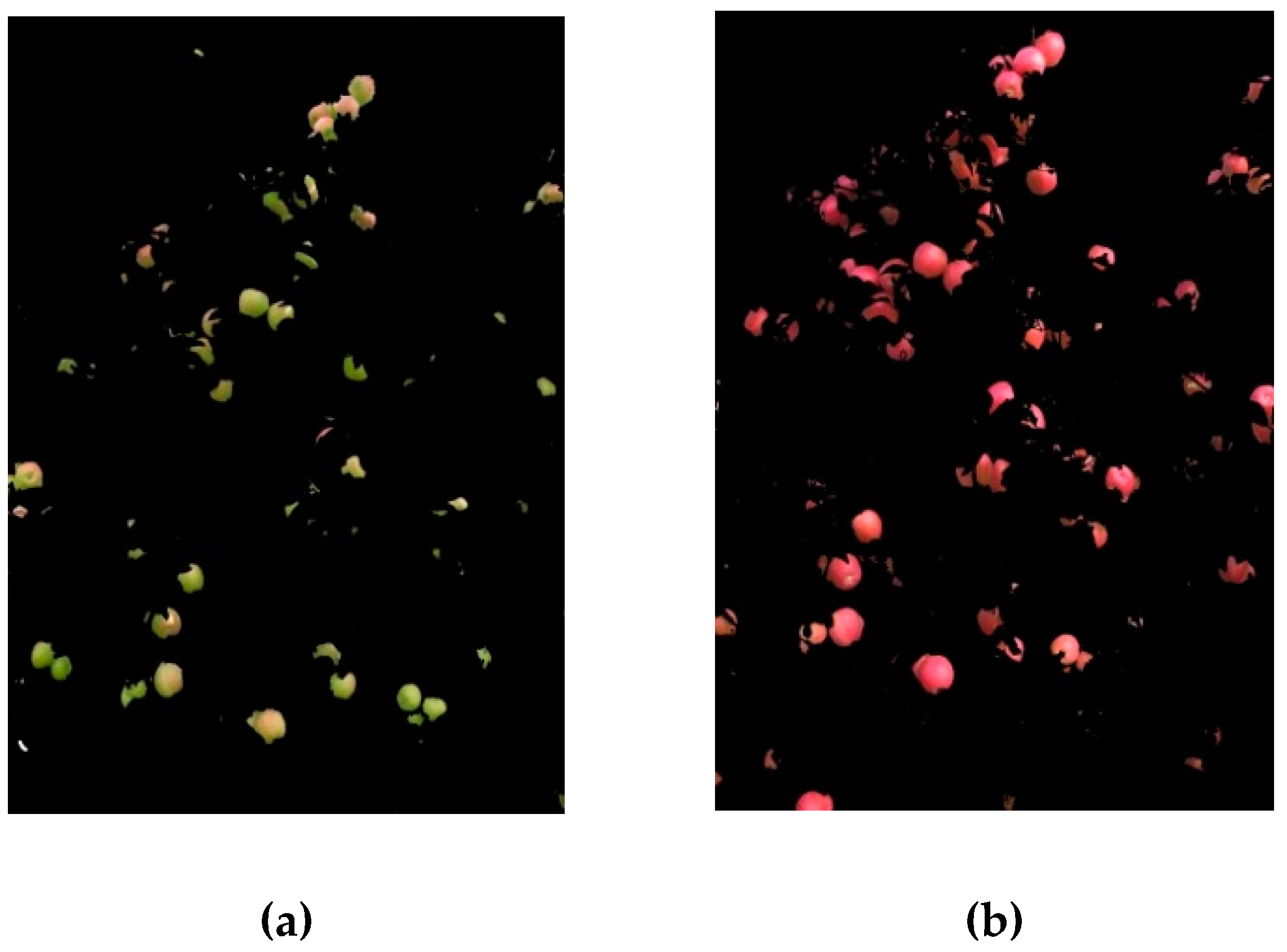
The objective of this study was to improve the accuracy of early yield prediction by taking features of the tree-canopy structure (number of fruit FN, area of fruits FA, area of fruit clusters FCA, and foliage leaf area (LA)) in the canopy image into account, besides the apple fruit number. The aims of the present paper are: (1) to describe the processes of extracting canopy features and “learning” the relationship between the features and actual yield per tree by use of a back propagation neural network (BPNN) using the data from 2009–2010; (2) to evaluate the BPNN prediction models to analyse the relation between the estimated and harvested apple yield; and (3) to represent the accuracy of the BPNN models by predicting the yield for 30 samples from 2011.

2. Materials and Methods

2.1. Site Description and Image Acquisition

Apple cv. ”Gala” trees, trained as slender spindles and spaced at a tree distance of 1.5 and a row distance of 3.5 m oriented North to South, were located at the University of Bonn, Campus Klein-Altendorf, Germany (50.6° N, 6.97° E, 180 m a.s.l.). The “Gala Model 1” was used to train and test 90 thirteen-year-old “Pinova” apple trees on dwarfing M9 rootstock, spaced also at 3.5 m × 1.5 m and also trained to slender spindles after June drop in 2012. In 2013, the model was used to predict the yield of 30 samples of “Pinova” apple trees, which were captured during the same period.
The soil is a rich luvisol on alluvial loess with a score of 92 on a 100 point soil fertility scale. The climate is dominated by Atlantic Western weather buffered by the mild Rhine river influence and 604 mm annual rainfall, thereby not requiring any irrigation. A total of 180 images were captured at 1.5 m height and at a constant distance of 1.4 m perpendicular to each tree row in natural daylight using a commonly available digital camera type Samsung (Seoul, South Korea) VB 2000 with German Schneider (Green Bay, WI, USA) lens with automated white calibration in “auto-focus” mode (without the use of the zoom) set to 3 Megapixels per image. White and red calibration spheres of 50 mm diameter (polystyrene) were used to determine fruit size. A 2 m × 3 m white drapery cloth was placed behind the target tree to distinguish fruits from trees in other rows. Images (Table 1) were captured twice, i.e., when fruit were light-green after June drop about three months before harvest (period 1; “Gala Model 1”) and when fruit were red during the fruit ripening period half a month before harvest (period 2; “Gala Model 2”), on the preferred western side of the tree. Illumination for the first image acquisition was estimated ca. 800 µmol PAR and for the second date ca. 600 µmol PAR m−2·s−1 using an EGM-5 (PPSystems, Amesbury, MA, USA). Images were obtained on these apple trees, in the early afternoon (3 to 5 pm) on days with indirect light to exclude stray or blinding light, and deep shades at a time of low solar angle on the second date (period 2).
After harvest, fruit were sorted using a commercial grading machine (type MSE2000, Greefa, Geldermalsen, The Netherlands) to provide fruit, counts for each individual tree, size for each individual fruit, and cumulative yield/tree.
Matlab (version 2011b, Mathwoks Inc., Natik, MA, USA) was used for the image processing and modeling. Typical images are shown in Figure 1. To improve the data processing speed, images were uniformly resized to 512 × 683 pixels. The parameters used in this paper, are listed in Table 2.

2.2. Apple Fruit and Leaf Feature Description

Fruit and foliage are two main components of the apple tree canopy. Based on the images of the apple tree canopy, the fruit number (FN) and the fruit area (FA) are the first two essential features for yield prediction. The third feature is the area of the apple clusters (FCA) in the image, because apple clusters are a conspicuous characteristic of canopy structure, which can be comprised of more than two apples. Compared with the pixel proportion of the bright red calibration sphere (Figure 1a), which was of the size range for an apple fruit in period 1, if the fruit domain exceeded the size of the calibration sphere by 3-fold, it was assumed to be an apple cluster. Since the leaves can impact apple yield estimation by occluding fruit, foliage area (LA) is the fourth one.
As we consider FA, FN, LA, and FCA extracted from canopy images as essential parameters for yield prediction [5], we converted them to the ratios F1, F2, F3 and F4 (Table 2). These ratios were subsequently employed for modelling and the different steps in the modelling process are visualized in a flowchart (Figure 2).

2.3. Fruit Identification and Feature Extraction (Step 1)

The implemented fruit recognition algorithms were based on a previous study [5] (Figure 3). The RGB images were transformed to a binary image and analysed to count the apples within the picture. Pixels of each connected domain were summed as its area to computed FA, FN and FCA.

2.4. Leaf Identification and Feature Extraction (Step 2)

A method was developed for automated recognition of foliage within the tree image. Before foliage identification, the fruit domains were removed from the canopy image (Figure 4). Both RGB and HSI colour systems were used to segment leaves in the image automatically. Figure 4 gives an overview in order of image processing. The proposed method was employed to separate foliage from the background (white drapery, branches and sky) in the image.
The map of colour difference (green minus blue, i.e., G − B) for each pixel is shown in Figure 5. The green minus blue value was larger for the foliage compared with the background (white drapery and sky), which could be used to segment foliage from the image at a threshold colour difference G-B of 10. For each pixel, if the colour difference was below 10, then the R, G, B colour values of this pixel were set to zero (Figure 4).
However, background pixels (branches and trunk) were incorrectly assigned the same classification as foliage pixels. Specifically, in the hue (H) image, the pixels were divided into two classes (Figure 4), and one of them consisted of the deeper colour pixels represented by branches and trunk. Eventually, using the Ostu’s algorithm [12], a threshold (T) was obtained. The branches and trunk were removed from the image at the threshold T. Foliage cross-sectional area (LA) was computed by summing pixels that belonged to foliage.

2.5. Development of BPNN Yield Prediction Model (Step 3)

The ratios F1, F2, F3, F4 and F5 (Table 3) were computed based on the parameters IA, FA, FN, FCA, LA and YA (Table 2). One data set of 150 images acquired in period 1 was collected as set 1, and the other set of 150 images acquired in period 2 was collected as set 2. Sixty images were sampled in the summer of 2009 and ninety images were sampled in the summer of 2010 for the two sets, i.e., each set included 150 samples, respectively. Each sample consisted of five parameters. Two BPNN prediction models were built for the two periods using Sets 1 and 2, respectively.
The Back Propagation Neural Network (BPNN) was trained with an error back-propagation learning algorithm used for computing the ANN weights and biases [13]. In this present study, the inputs were the four features from the apple tree image and a vector of features in BPNN, which were different from that of Rozman [6], and the output was the forecast yield. As BPNN was trained, the weights of inputs for each processing unit were adjusted, and the network gradually “learned” the input/output relationship to minimize MSE between the actual yield of an apple tree and the estimated yield of the sample set.
A typical three-layer BPNN with one input layer, one hidden layer, and one output layer was employed in our present study. To determine the optimal number of hidden neurons, the number of hidden neurons was initially calculated as Equation (1), and the value of NA was adjusted to select the best one based on the minimization of the mean squared errors (MSE), which is a statistical measure showing how well the model predicts the output value and the target value (yield).
N H = ( N I + N O ) 1 / 2 + N A , N A [ 0 , 10 ]
-
NI is the number of input neurons,
-
NO is the number of output neurons,
-
NH is the number of hidden neurons,
-
NA is the number of the neurons, which can be added in hidden neurons based on MSE.
Before BPNN training, the main parameters were set (Table 4). In order to reduce extra or over-fitting of the 150 samples, 90% of the samples composed the training set, which was used to develop the model, and the remaining 10% was used for the test set [14]. Both the training and test set were selected randomly, guaranteeing a balanced proportion between positive and negative outcomes. During BPNN training, the target parameter and the inputs were all inserted into the neural network. Each node in the input and hidden layers were connected to each of the nodes in the next layer (hidden or output). All connections between nodes were directed (i.e., the information flows only one way), and there are no connections between the nodes within a particular layer. Each connection between nodes had a weighting factor. These weighting factors were modified using the back-propagation algorithm based on the “error” during the training process to produce “learning”.

2.6. The Measures for Model Evaluation

Four statistical approaches were employed to evaluate the model: R2, MFE, RMSE, and MAPE. Mean Forecast Error (MFE) is a measure of unbiasedness of the predictions, defined as Equation (2), and MFE is closer to 0, then the model becomes less unbiased. Root mean squared error (RMSE) is an often used measure of the difference between values predicted by a model and those actually observed from the object being modeled, and is defined as Equation (3). It can rule out the possibility that large errors of opposite signs could cancel out in a MFE measure. The Mean Absolute Percentage Error (MAPE) is computed through a term-by-term comparison of the relative error in the prediction with respect to the actual value of the variable, and is defined as Equation (4). Thus, the MAPE is an unbiased statistical approach for measuring the predictive capability of a mode [14,15].
M F E = 1 N N ( Y A Y E )
R M S E = 1 N N ( Y A Y E ) 2
M A P E = N | ( Y A Y E ) / Y A | × 100 N

3. Results

3.1. Data Analysis

The objective of the work was to evaluate algorithms for the detection of young light green apple fruit three months before harvest as accurately as possible. As shown in Table 3 for the same apple tree, the canopy feature values were developed from July (period 1) to September (period 2). In period 1, when the apple fruit was small, the computed values (fruit-related ratios) of F1, F2, and F3 were much smaller compared with the foliage-related ratio F4; in period 2, the values of F1, F2, and F3 increased with increasing fruit size. Therefore, the fruit detection is strongly dependent on the amount of foliage in the canopy, which makes it almost impossible to detect apple fruit using image analysis in period 1. In period 2, the obvious colour and size changes of apple fruits make the detection easier and the influence of the foliage becomes weak. Overall, F1 appears to be the most important parameter, because it reflects the area of all apples in the tree image. Hence, it includes the overall information on the size and number of all apples.

3.2. BPNN Model Structure and Validation

The BPNN “Prediction Model 1” for the early period after June drop consists of 4 input neurons, 12 hidden neurons and 1 output neuron, and the BPNN “Prediction Model 2” for the ripening period consists of 4 input neurons, 11 hidden neurons, and 1 output neuron.
Both models performed well relative to each other, and illustrate that ANN could be employed to predict the apple yield. Table 5 shows the small differences between the early and late yield prediction model for cv. “Gala” regarding R2 (0.02), RMSE (0.15 kg/tree), MFE (0.02), and MAPE (0.45 %), and shows that the results of Model 1 (Table 5) were similar to those of Model 2 (Table 6) with Model 1 being slightly inaccurate.

3.3. Yield Prediction for Subsequent Year

To evaluate their reliability and robustness, the two BPNN yield prediction models, based on combining both the 2009 and 2010 data, were used to predict the yield for next year (2011). In the growing season of 2011, 30 trees (Table 1) were selected for a wide variability of fruit load and were photographed in July and September as samples to validate the performance of “Prediction Model 1” and “Prediction Model 2”, respectively. The results indicate the two models have good reliability and robustness, and the correlation increased from 0.62 to 0.75 near harvest time (Figure 6).

3.4. Yield Prediction for Other Apple Varieties

The results (Table 7 and Table 8) shows that the “Pinova” model performs similar to the “Gala” model 1. This “Pinova” model also could be used to predict the yield for the subsequent year (Figure 7). These again proved that a BPNN model, based on the features from the canopy, could be used for apple yield prediction at the orchard level.

4. Discussion

The majority of studies have used image processing algorithms to estimate total fruit number and fruit diameters to achieve yield prediction shortly before the fruit maturity and harvest [16,17,
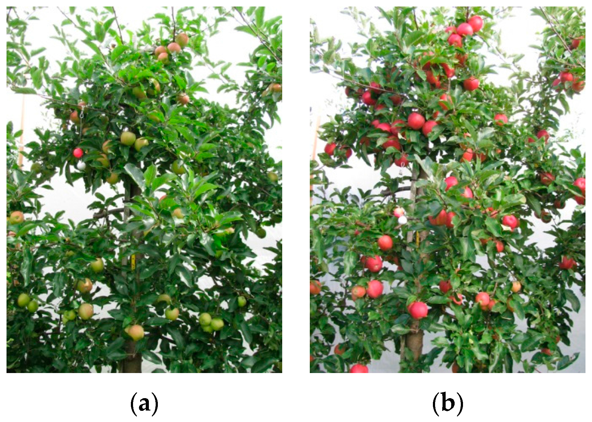
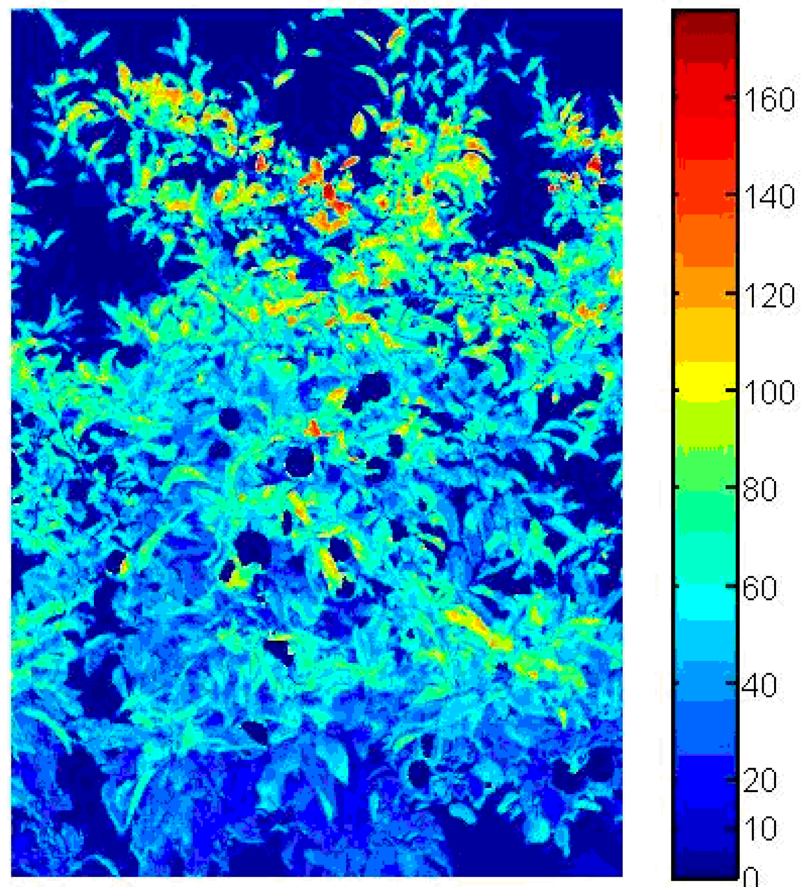
18]. However, counting the number and measuring the size of fruit by machine vision is based on the premise that all fruit on a tree can be seen and are not occluded by leaves. The scientific challenge is to identify each fruit in the tree image with some fruit hidden within the canopy, especially in the early period (
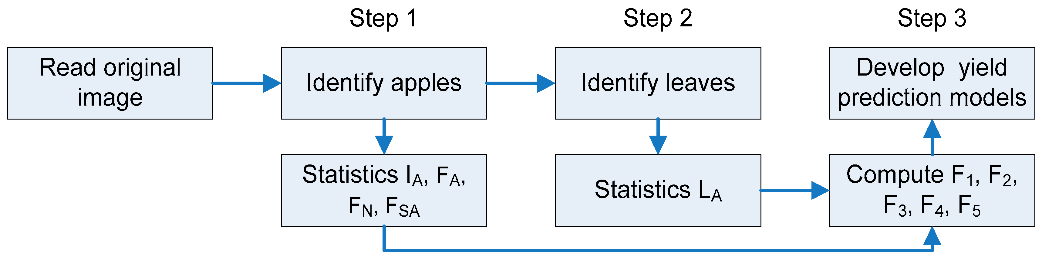
Figure 1a). However, early prediction is essential for planning labor, bins, and harvest organization as well as transport, grading, and storage. Hence, four features were extracted from the tree image (Table 2), which were closely related to yield prediction and, moreover, changed with the growth of the fruit (Table 3). BPNN was employed for the analysis of the relationship between the four features and the actual yield to model yield prediction (Figure 6).
The small differences between the early and late yield prediction model for cv. “Gala” in Table 5 could be attributed to the fact that the proposed method with the neural network, based on the features from canopy images, can reduce the adverse influence from foliage. Hence, the method could be used for apple yield prediction in early and late growing periods after June drop, even when the apple fruit are small and green. In Table 6, the small differences between the harvested and the predicted yield for both models suggest that the BPNN model based on the features of canopy could provide accurate apple yield prediction at the individual orchard level.
In the two BPNN models for early prediction in July and pre-harvest in September, four features were extracted from the tree canopy image from the respective period as inputs into the model, and the apple yield can then be predicted. This approach with a resolution of 2.4 and 2.3 kg/tree apples (Table 5) is a further advancement to the ANN model of Rozman et al. [6], in which the numbers of fruits at different times (the time between June drop to near harvest time was divided into several periods) are input parameters resulting in a RMSE of 2.6 kg/tree for cv. “Braeburn” and 2.8 kg/tree for “Golden Delicious” both in September, possibly too short before harvest of these late ripening varieties to organize labour and bins.
In previous research, Zhou et al. [5] showed that R2 values in the calibration data set between apple yields estimated by image processing and actual harvested yield were 0.57 for young cv. “Gala” fruit after June drop, which improved to R2 = 0.70 in the fruit ripening period. By comparison, the presented combined approach (Table 5) improved the coefficient of determination (R2) for young, small, and light-green cv. “Gala” fruit to 0.81 and for ripening fruit to 0.83. This is also an advancement of the results of Rozman et al. [6] with a correlation (r) between the forecast and actual yield of r = 0.83 for “Golden Delicious” and 0.78 for “Braeburn”, with standard deviations (SD) of 2.83 and 2.55 kg. In our study, R² was 0.81 and SD was 2.28 kg for “Gala” (Table 5).
Other work concentrated on optimising recognition of green apple fruit cv. “Golden Delicious”, but without yield prediction [8,18], while Cheng et al. [19] showed how yield estimation strictly depends on the crop load of the apple tree.
Aggelopoulou et al. [20] estimated the yield of apple trees based of flower counts, a method which is only suitable for med-climates such as Greece. However, the majority of apple growing countries in Northwestern Europe such as Germany, Belgium, Holland, England, and Poland encounter late frost, which can dramatically reduce the yield, accentuated by an unpredictable June drop with the same effect, making proper yield predictions before June drop impossible.
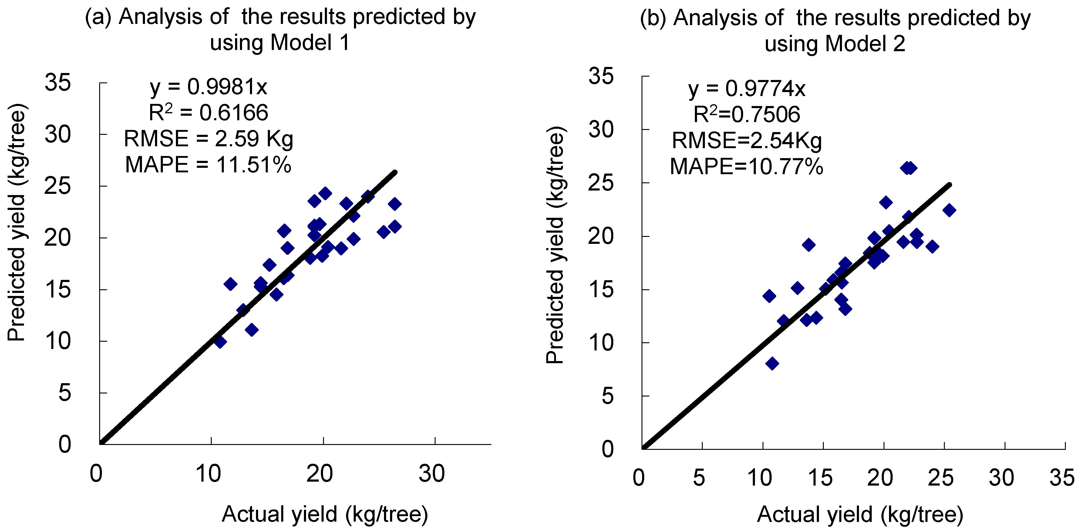
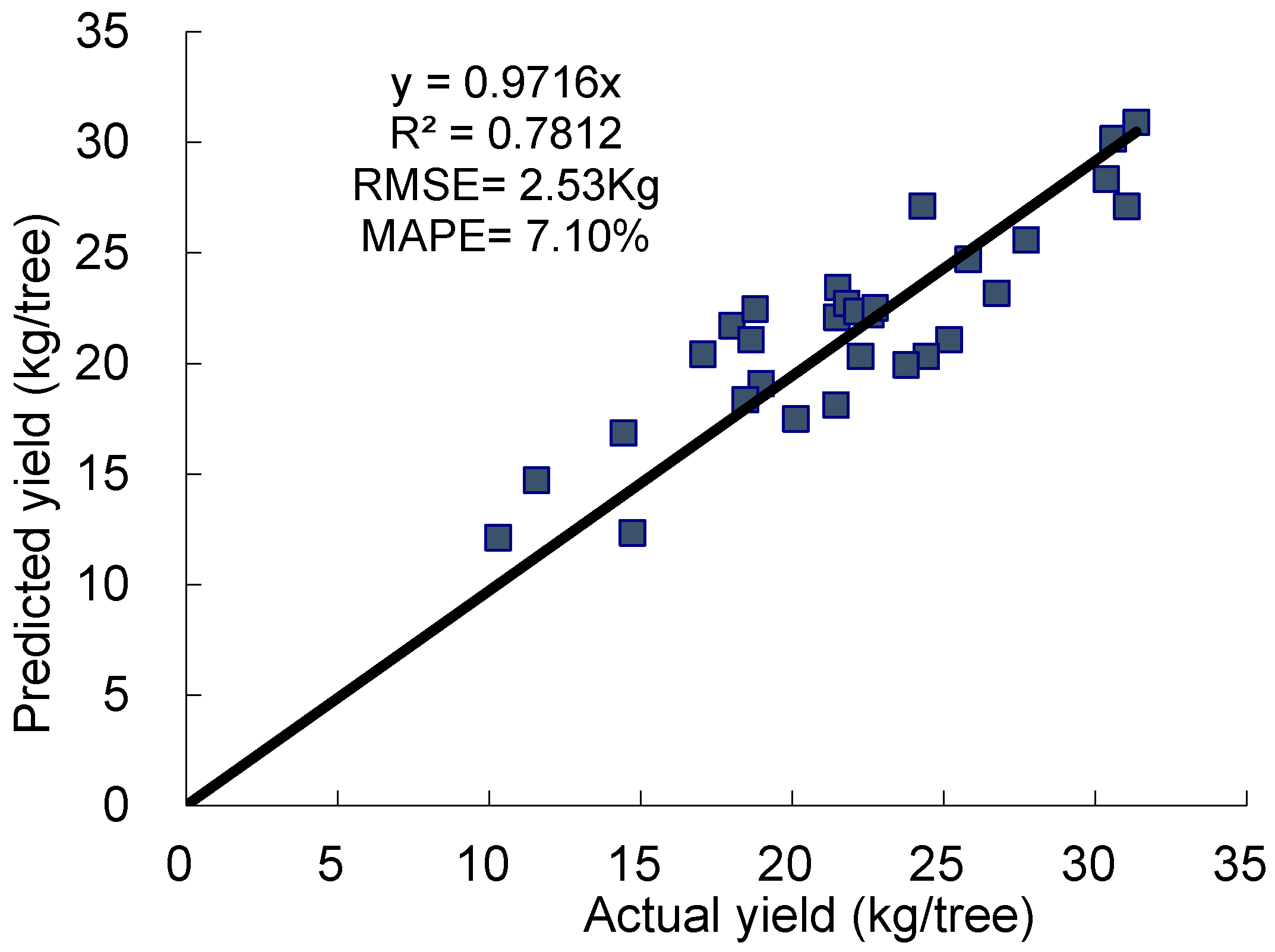
The results shown in Figure 7 validated the practicability of the models. The RMSE values between estimated apple yield and actual harvested yield was 2.6 kg/tree for the early time, and improved at near harvest time to 2.5 kg/tree. The BPNN model trained with the samples of 2009 and 2010 and with the tree images in July 2011 can be used to predict the yields of apple trees from 2011.
Further research will show where and why we under- or over-estimate the fruit yields per tree. The tree shape employed here, slender spindle, should allow similarly good results with similar tree shapes such as tall, spindle, super spindle, fruit wall, and Solaxe tree training systems.

5. Conclusions

The novelty of the approach is the combination of fruit features with (four) tree canopy features (number of fruit FN, single fruit size FA, area of fruit clusters FCA, and foliage leaf area (LA)) to develop two back propagation neural network (BPNN) models for early yield prediction, i.e., for young, small, green fruitlets and mature red fruits. Apple was used as a model fruit or crop and the algorithms were developed for image acquisition under natural light conditions in the orchard. The results showed that BPNN can be used for apple yield prediction and that those four selected canopy features are suitable for early yield prediction and present an elegant way for predicting fruit yield using machine vision and machine learning for apple and possibly other fruit crops.

6. Outlook

The present work was obviously conducted in our own orchard with apple trees as slender spindles, as typical for this growing region, to develop these algorithms. Hence our next project will focus to separate a site-specific model from a general model and investigate the adaptation of the proposed model to other tree forms or similar fruit such as nectarine, peach, or kaki.

Acknowledgments

We are grateful to the Chinese-German Center for Scientific Promotion (Chinesisch-Deutsches Zentrum für Wissenschaftsförderung) under the project of the Sino-German Research Group (GZ888), the German Academic Exchange Service (DAAD), and the China Scholarship Council (CSC) for supporting our bi-lateral cooperation, and MDPI for the invitation to this special edition of the J Imaging.

Author Contributions

As part of her PhD study, Hong Cheng carried out the experiments partly at the University of Bonn and partly in China under the supervision of Yurui Sun at China Agricultural University Beijing. Lutz Damerow provided the technical setup, while the image acquisition and most of the writing, publication, and horticultural input was contributed by the corresponding author Michael Blanke.

Conflicts of Interest

The authors declare no conflict of interest.

Abbreviations

The following abbreviations are used in this manuscript:
ANNArtificial neural network
BPNNback propagation neural network

References

  1. Wulfsohn, D.; Zamora, F.A.; Téllez, C.P.; Lagos, I.Z.; Marta, G.F. Multilevel systematic sampling to estimate total fruit number for yield forecasts. Precis. Agric. 2012, 13, 256–275. [Google Scholar] [CrossRef]
  2. Stajnko, D.; Rakun, J.; Blanke, M. Modelling apple fruit yield using image analysis for fruit colour, shape and texture. Europ. J. Hortic. Sci. 2009, 74, 260–267. [Google Scholar]
  3. Wachs, J.P.; Sturm, H.J.; Burks, F.; Akhanais, V. Low and high-level visual feature-based apple detection from multi-modal images. Precis. Agric. 2010, 11, 717–735. [Google Scholar] [CrossRef]
  4. Blanke, M.M. Prediction of apple yields in Europe—Present and new approaches in research. In Proceedings of the 106th Annual Meeting of the Washington State Horticultural Association (WSHA), Yakima, WA, USA, 8–10 December 2011; Smith, L., Ed.; WSHA Publishing: Yakima, WA, USA, 2011; pp. 68–75. [Google Scholar]
  5. Zhou, R.; Damerow, L.; Sun, Y.; Blanke, M. Using colour features of cv. ‘Gala’ apple fruits in an orchard in image processing to predict yield. Precis. Agric. 2012, 13, 568–580. [Google Scholar] [CrossRef]
  6. Rozman, C.; Cvelbar, U.; Tojnko, S.; Stajnko, D.; Karmen, P.; Pavlovie, M.; Vracko, M. Application of Neural Networks and Image Visualization for Early Predicted of Apple Yield. Erwerbs-Obstbau 2012, 54, 69–76. [Google Scholar]
  7. Stajnko, D.; Rozmana, Č.; Pavloviča, M.; Beber, M.; Zadravec, P. Modeling of ‘Gala’ apple fruits diameter for improving the accuracy of early yield prediction. Sci. Hortic. 2013, 160, 306–312. [Google Scholar] [CrossRef]
  8. Kelman, E.; Linker, R. Vision-based localisation of mature apples in trees images using convexity. Biosyst. Eng. 2014, 118, 174–185. [Google Scholar] [CrossRef]
  9. Ye, X.; Sakai, K.; Garciano, L.O.; Asada, S.I.; Sasao, A. Estimation of citrus yield from airborne hyperspectral images using a neural network model. Ecol. Model. 2006, 198, 426–432. [Google Scholar] [CrossRef]
  10. Linker, R.; Cohen, O.; Naor, A. Determination of the number of green apples in RGB images recorded in orchards. Comput. Electron. Agric. 2012, 81, 45–57. [Google Scholar] [CrossRef]
  11. O'Neal, M.R.; Engel, B.A.; Ess, D.R.; Frankenberger, J.R. Neural network prediction of maize yield using alternative data coding algorithms. Biosyst. Eng. 2002, 83, 31–45. [Google Scholar] [CrossRef]
  12. Sezgin, M.; Sankur, B. Survey over image thresholding techniques and quantitative performance evaluation. J. Electron. Imaging 2004, 13, 146–165. [Google Scholar]
  13. Rumelhart, D.E.; Hinton, G.E.; Williams, R.J. Learning Representations by Back-Propagating Errors. Nature 1986, 323, 533–536. [Google Scholar] [CrossRef]
  14. Esmaeili, A.; Tarazkar, M.H. Prediction of shrimp growth using an artificial neural network and regression models. Aquac. Int. 2010, 19, 705–713. [Google Scholar] [CrossRef]
  15. Greene, W.H. Econometric Analysis, 4th ed.; Prentice-Hall: Englewood Cliffs, NJ, USA, 2000; p. 1007. [Google Scholar]
  16. Annamalai, P.; Lee, W.S.; Burks, T. Color Vision Systems for Estimating Citrus Yield in Real-Time. In Proceedings of the ASAE/CSAE Annual International Meeting, Ottawa, ON, Canada, 1–4 August 2014.
  17. Lee, W.S.; Chinchuluun, R.; Ehsani, R. Citrus fruit identification using machine vision for a canopy shake and catch harvester. Acta Hortic. 2009, 824, 217–222. [Google Scholar]
  18. Zaman, Q.U.; Schumann, A.W.; Percival, D.C.; Gordon, R.J. Estimation of wild blueberry fruit yield using digital color photography. Trans. ASABE 2008, 51, 1539–1544. [Google Scholar] [CrossRef]
  19. Cheng, H.; Damerow, L.; Sun, Y.; Blanke, M.M. Detection of apple fruit in an orchard for early yield prediction as dependent on crop load. Acta Hortic. 2016, 1137, 59–66. [Google Scholar] [CrossRef]
  20. Aggelopoulou, A.D.; Bochtis, D.; Fountas, S.; Swain, K.C.; Gemtos, T.A.; Nanos, G.D. Yield prediction in apple orchards based on image processing. Precis. Agric. 2011, 12, 448–456. [Google Scholar] [CrossRef]
Figure 1. Sample apple tree at different times; left picture (a) was acquired in the early period after the June drop (period 1), about 3 months before harvest, right picture (b) was acquired during the ripening period (period 2), about 15 days before harvest.
Jimaging 03 00006 g001
Figure 2. Outline of the processing steps.
Jimaging 03 00006 g002
Figure 3. Image of same tree at different times, (a) in July; (b) in the beginning of September.
Jimaging 03 00006 g003
Figure 4. Proposed algorithm for leaf discrimination; an example of image processing.
Jimaging 03 00006 g004
Figure 5. Example of an image of an apple tree with colour-coded mapping of colour differences between G (green) and B (blue) for each pixel, showing the leaves as bright colour dots and the background in deep blue.
Jimaging 03 00006 g005
Figure 6. Yield prediction for 2011 based on (a) “Prediction Model 1” for young apple fruit in July and (b) “Prediction Model 2” for ripe apple fruit in September for the subsequent year (n = 30 trees).
Jimaging 03 00006 g006
Figure 7. Yield prediction for 2013 based on the prediction “Pinova” Model for young apple fruit in July for the subsequent year (n = 34 trees).
Jimaging 03 00006 g007
Table 1. Characteristics of samples. Tree fruit load % refers to the % of trees carrying a high (>mean + SD), low (<mean − SD), and moderate fruit load, respectively.
SeasonNumbers of TreesNumber of Images (Period 1, Period 2)Yield/Tree (mean ± SD)Tree Fruit Load (%) High, Mod, Low
20096060; 6020.62 ± 4.9020; 68; 12
20109090; 9016.68 ± 5.4318; 63; 19
2009 & 2010150150; 15018.26 ± 5.5515; 67; 18
20113030; 3018.63 ± 4.1710; 70; 20
Table 2. Description of parameters for yield prediction.
ParameterDescriptionParameterDescription
IASum of pixels of the whole imagesYEThe estimated yield of apple tree
FASum of pixels belonging to apple fruits F1FA/IA
FNNumber of fruitF2FN/200
FCASum of pixels belonging to apple clustersF3(FA– FCA)/IA
LASum of pixels belonging to foliageF4LA/IA
YAThe actual yield of apple treeF5YA/50
MAPEMean Absolute Percentage ErrorSDStandard deviation of the error
MFEMean Forecast ErrorRMSERoot Mean Square Error
Note: the fruit number per tree is below 200; the actual yield per tree is below 50 kg.
Table 3. Example of 15 trees for modelling.
SetsSet 1Set 2
Tree F1F2F3F4F5F1F2F3F4F5
10.01590.31000.01590.54950.45710.05520.51000.03310.22780.4571
20.00410.18000.00410.42650.33550.02790.38500.02420.21000.3355
30.01030.31000.01030.47180.38080.03480.49000.01990.19000.3808
40.00880.25500.00880.72450.36790.03470.61000.01990.20520.3679
50.02140.52500.01930.70220.44230.05900.55000.02970.20660.4423
60.00810.38500.00810.57140.45090.03180.53500.02510.23720.4509
70.01080.40000.00600.50240.36110.03200.47000.01590.18930.3611
80.01250.37500.01250.73440.36480.04400.54000.03290.20840.3648
90.00600.31000.00600.40660.51060.05490.50000.03270.33600.5106
100.01490.39000.01490.75590.38630.05370.51000.03290.21010.3863
110.01910.45500.01700.71160.44310.05960.43500.03400.19020.4431
120.00960.33500.00960.41490.39440.04450.57500.02690.17530.3944
130.01440.41500.01440.70990.41310.05460.39000.02290.25930.4131
140.01800.31500.01480.64590.35260.05850.38500.01730.16630.3526
150.00410.18000.00410.42650.33550.02790.38500.02420.21000.3355
Table 4. Relative parameter settings before the training BPNN.
ParameterValueParameterValue
InputF1, F2, F3, F4Hidden layer transfer functionLogarithmic sigmoid transfer function
TargetF5Output layer transfer functionLinear transfer function
OutputForecast valueLearning functionGradient descent learning function
Performance functionMSETraining functionLevenberg-Marquardt back-propagation
Table 5. The model structure and the evaluation of model performance for cv. “Gala”.
ParameterStructureSamples (Trees) of 2009 and 2010RMSE in kg/TreeMAPE (%)MFER2
Model
Model 1Train set4-12-11352.3410.67−0.050.81
Test set152.5312.400.160.80
Model 2Train set4-11-11352.278.9−0.030.83
Test set152.3110.36−0.060.82
Table 6. Comparison between actual yield and predicted yield; n = 150 trees.
ModelActual Yield (A) in kg per 150 TreesPredicted Yield (P) in kg per 150 TreesDifference (|A – P|) in kgMean Difference in kg per Tree
Model 12736274480.05
Model 22736274040.03
Table 7. The model structure and the evaluation of model performance which was developed based on samples of 2012 for cv. “Pinova”.
ParameterStructureSamples (Trees) of 2012RMSE in kg/TreeMAPE (%)MFER2
Model
“Pinova” Model Train set 4-10-1802.2411.45−0.140.89
Test set102.5314.190.060.88
Table 8. Comparison between actual yield and predicted yield for 2012; n = 90 trees.
ModelActual Yield (A) in kg per 100 TreesPredicted Yield (P) in kg per 100 TreesDifference (|A–P|) in kgMean Difference in kg per Tree
“Pinova” Model1817182250.06

