
On the Applicability of Transfer Function Models for SSI Embedment Effects


1
European Centre for Training and Research in Earthquake Engineering (EUCENTRE), Via Adolfo Ferrata 1, 27100 Pavia, Italy
2
National Laboratory for Civil Engineering (LNEC), Av. Do Brasil 101, 1700-066 Lisboa, Portugal
3
Department of Civil Engineering and Architecture, University of Pavia, Via Adolfo Ferrata 5, 27100 Pavia, Italy
*
Author to whom correspondence should be addressed.
Infrastructures 2021, 6(10), 137; https://doi.org/10.3390/infrastructures6100137
Submission received: 31 August 2021
/
Revised: 14 September 2021
/
Accepted: 19 September 2021
/
Published: 24 September 2021
(This article belongs to the Special Issue Seismic Reliability Assessment and Advances in Structural Modelling)
Abstract
:Soil-structure interaction (SSI) effects are typically neglected for relatively lightweight buildings that are less than two-three storeys high with a limited footprint area and resting on shallow foundations (i.e., not featuring a basement). However, when the above conditions are not satisfied, and in particular when large basements are present, important kinematic SSI may develop, causing the foundation-level motion to deviate from the free-field one due to embedment effects. In the literature, transfer function models that estimate the filtering effect induced by rigid massless embedded foundations are available to “transform” foundation-level recordings into free-field ones, and vice-versa. This work describes therefore a numerical study aimed at assessing potential limits of the applicability of such transfer functions through the employment of a 3D nonlinear soil-block model representing a layered soil, recently developed and validated by the authors, and featuring on top a large heavy building with basement. A number of finite element site response analyses were carried out for different seismic input signals, soil profiles and embedment depths of the building’s basement. The numerically obtained transfer functions were compared with the curves derived using two analytical models. It was observed that the latter are able to reliably predict the embedment effects in “idealised” soil/input conditions under which they have been developed. However, in real conditions, namely when a non-homogeneous profile with nonlinear behaviour under a given seismic excitation is considered, especially in presence of a basement that is more than one storey high, they may fail in capturing some features, such as the frequency-dependent amplification of the motion at the basement level of a building with respect to the free-field one.
1. Introduction
Soil-structure interaction (SSI) effects are typically neglected for relatively lightweight buildings that are less than two-three storeys high with a limited footprint area and resting on shallow foundations (i.e., not featuring a basement). In fact, recordings obtained from instruments adequately installed inside these buildings are deemed to be representative of free-field motion (e.g., [1]). In the presence of large, heavy buildings, however, the foundation-level motion may significantly deviate from the free-field one, due to SSI effects. While it is known that both kinematic and inertial interaction contribute to SSI [2], the focus herein is on the former, and in particular on the perturbation of the free-field motion caused by the embedment effects in the presence of a basement. Estimation of the filtering effect induced by rigid massless embedded foundations typically involves the use of spectral acceleration ratios (e.g., [3]) or of transfer functions, the latter describing the ratio between the amplitude of the Fourier transforms of the foundation input motion, uFIM, and of the free-field surface motion, ug. Several transfer function models of this type exist in the current literature. These analytical expressions can be used, for instance, to correct motions recorded at the basement level of a building, thus allowing one to estimate the corresponding free-field motions. The latter are more suitable than foundation-level motions to develop new ground motion prediction equations (GMPEs) that are not biased by the presence of the structure [4].
The goal of this paper is to check the validity of such existing transfer function models for embedment effects, identifying their potential merits and limitations. It is known indeed that analytical models are valid, strictly speaking, only for homogeneous soil profiles and in the linear range. The use of average shear wave velocity (VS) in layered profiles and the presence of soil nonlinearity with energy dissipation (under sufficiently strong motions), among other issues, may lead these models to misrepresent the effects of embedment on the free-field motion. To check the models, a 3D nonlinear soil-block model representing a layered soil, recently developed and validated by the authors [1,5] and featuring on top a large heavy building with basement, was employed.
A finite element (FE) soil-block model allows for the implementation of the direct one-step SSI modelling approach, which is able to account simultaneously for kinematic and inertial interactions, as well as to handle soil nonlinearities. The current literature includes a number of works that use FE soil-block analyses to account for (linear or nonlinear) SSI. Some of these past works were aimed at evaluating the effects of SSI on the structural response by comparing different models that encompass soil-structure interaction with the fixed-base case taken as reference (e.g., [6]). The focus of other works was instead to assess if SSI effects could impact foundation-level recordings, which is also the focus of the current endeavour. Within the latter scope, Karatzetzou and Pitilakis (2018a) [7], using a 2D finite element soil-block model representing a linear homogeneous soil, observed that the peak acceleration of the foundation motion generally decreases with respect to the free-field one by 10%–15% on average for both squatty and slender structures and for soil profiles with soft to medium stiffness. They also observed that especially for short squatty structures resting on stiff soil profiles the foundation motion may also be amplified with respect to the free-field one. Karatzetzou and Pitilakis (2018b) [8] provided reduction factors in terms of ratios of maximum accelerations in foundation and free-field motions. Along the same lines, Conti et al. (2017) [9] investigated the filtering effect induced by kinematic interaction on rigid massless embedded foundations. Employing finite difference (FD) soil-block models (both 2D and 3D) representing a homogeneous isotropic viscoelastic soil, they proposed new simplified expressions for translational and rotational frequency-dependent transfer functions relating the foundation and free-field motions. Similar expressions can be found in the report by NIST (2012) [10] and in the study by Elsabee and Morray (1977) [11].
In this work, a number of finite element site response analyses were carried out for different seismic input signals, soil profiles and embedment depths of the building’s basement. In these analyses, the building’s total mass and weight were disregarded, so as to capture only the kinematic SSI effects; however, the actual stiffness of the structure and its basement/foundation was accounted for, together with the compression-only interface conditions between the latter and the surrounding soil. The obtained transfer functions, representing the ratio of foundation-level/free-field motions in the frequency domain, were then compared with those derived using the NIST (2012) [10] and Conti et al. (2017) [9] analytical models.
The manuscript is organised as follows. Section 2 describes the case study building with basement, the two soil profiles and the two earthquake recordings that were employed in the numerical analyses, while Section 3 presents the modelling approach adopted in OpenSees [12] for the soil-block and the structure. Section 4, after a brief state-of-the-art review on the transfer function models for embedment effects currently available, describes the two analytical models under investigation in this work, namely the ones proposed by NIST (2012) [10] and Conti et al. (2017) [9]. The final subsection presents the comparison between the FE-based transfer functions and the analytical ones, for several combinations of seismic input, soil profile and embedment depth. Conclusive discussions may then be found in Section 5.
2. Case Study Building, Soil Properties and Seismic Input
The comparison of transfer functions obtained from soil-block analyses with analytical expressions from the literature was carried out with reference to the case study building with basement, the two soil profiles and the two recordings briefly described in the following subsections.
2.1. Case Study Building with Basement
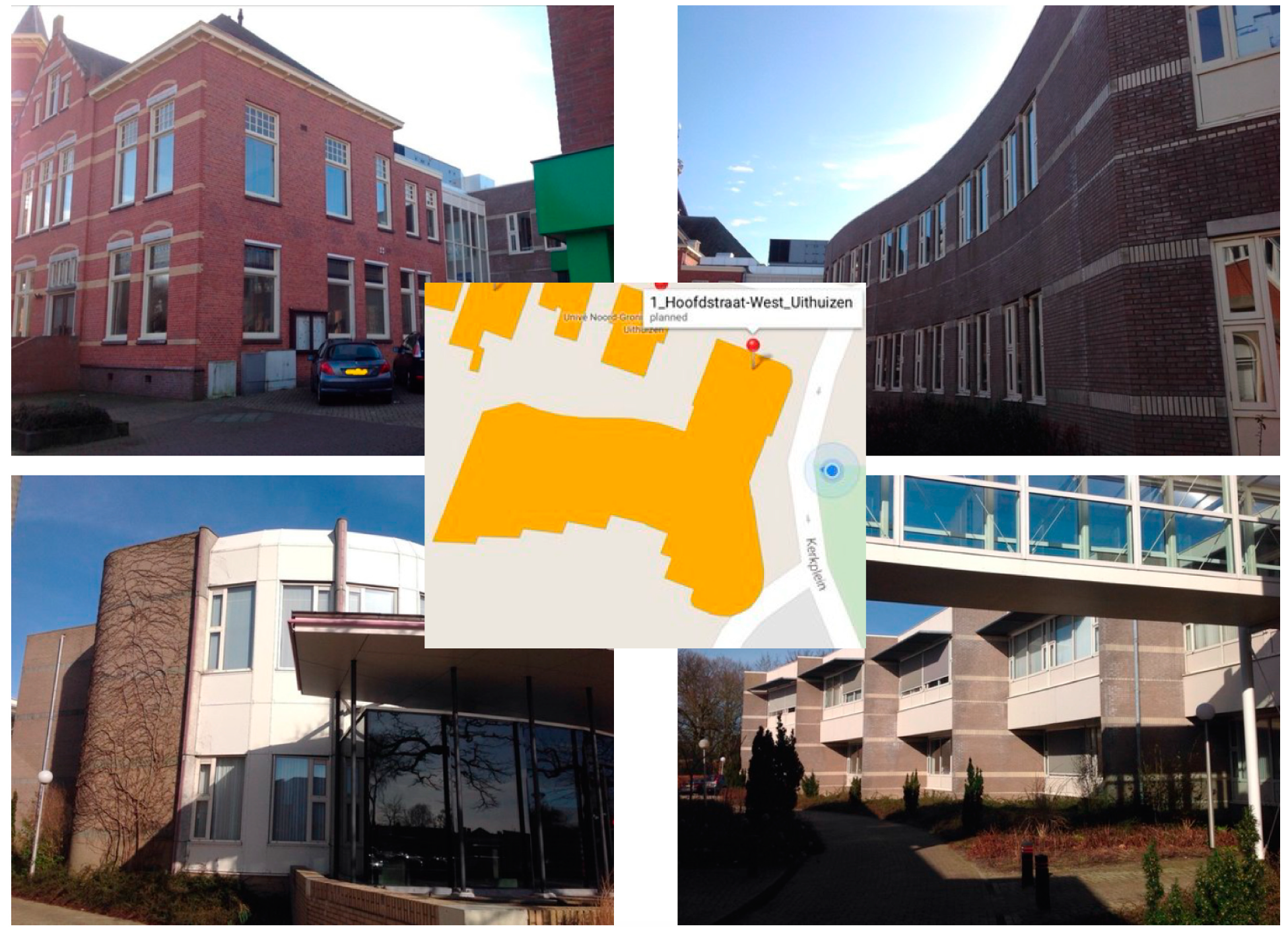
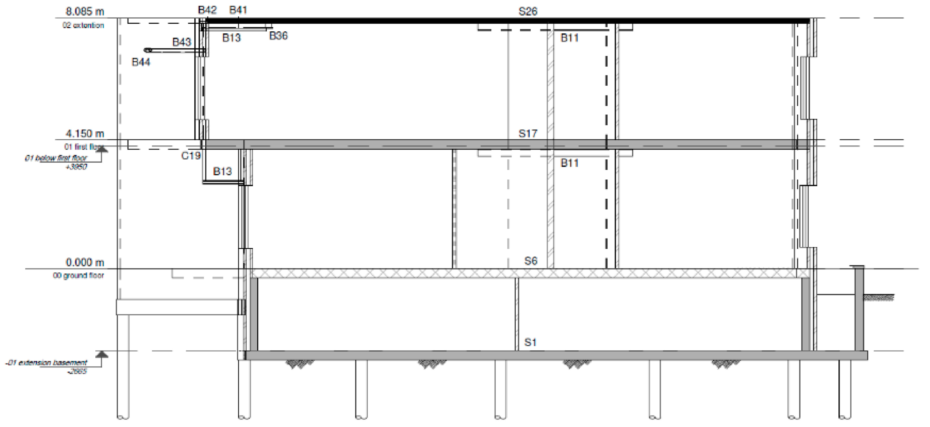
The city hall of Uithuizen (Figure 1), in the Northern Netherlands, was herein considered as a case study of building with a basement, as already done in [1]. The building is composed of different structures, of different ages and construction materials. In this work, only the portion corresponding to the structural drawing shown in Figure 2 was considered, with assumed plan dimensions of 16 × 16 m2. The structure features one underground storey of approximately 2.5-m depth, plus two storeys above ground, each around 4 m high. Floor slabs and the roof are made of timber, whereas the walls are in masonry and the foundation system consists of a slab on wooden piles. In order for the comparison to be more comprehensive and include responses obtained not only from different soil profiles and recordings, but also from varied structural configurations, two different embedment depths were considered herein for the same building, namely 2.5 m (i.e., the actual one) and 5 m.
2.2. Soil Properties
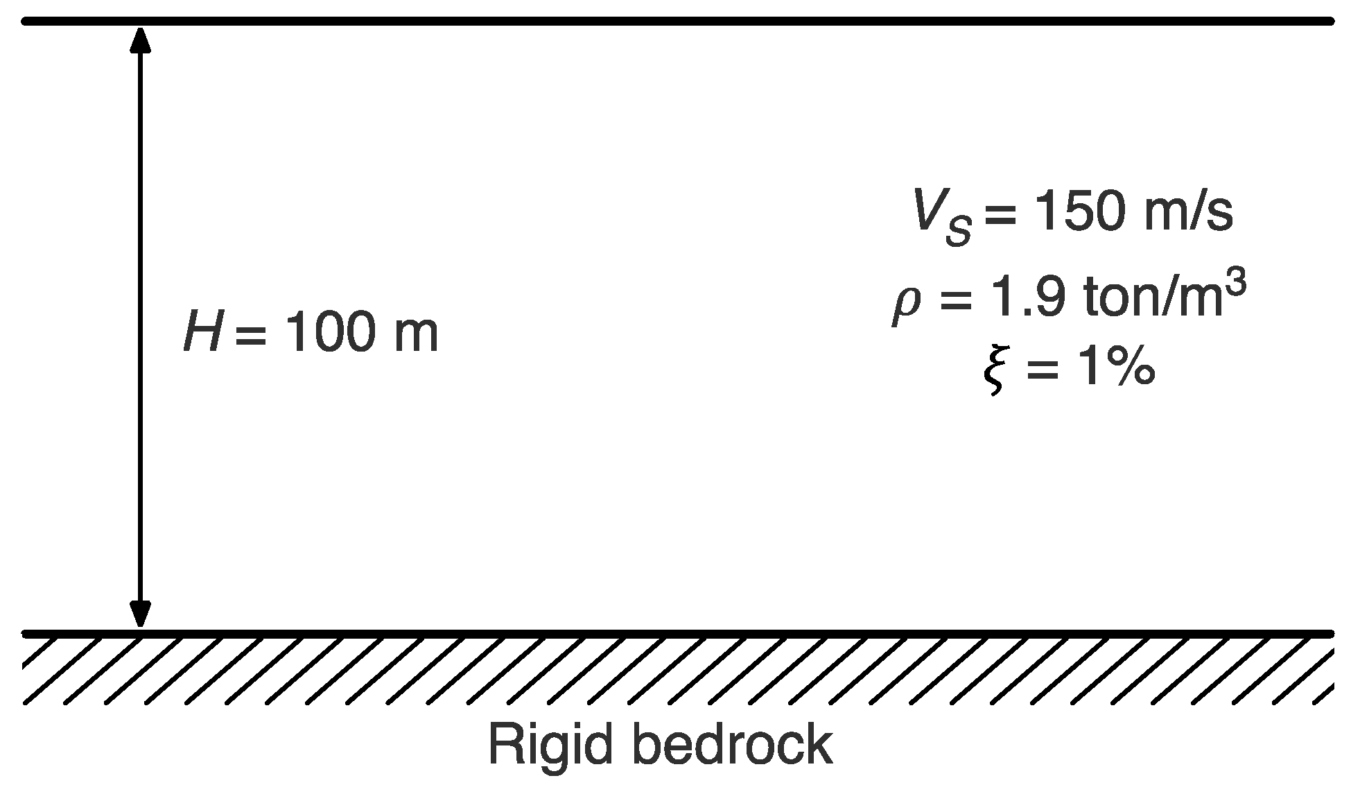
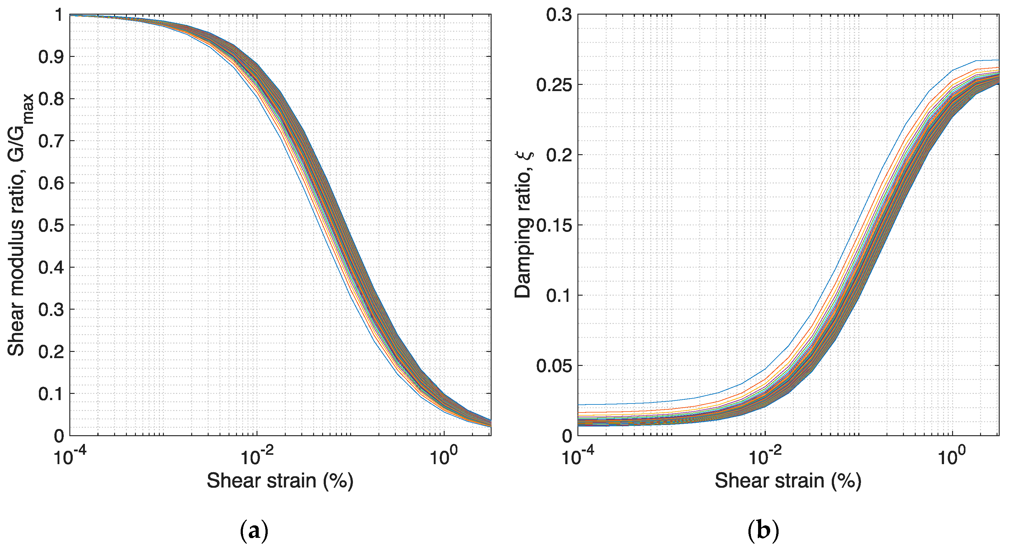
The first soil profile that was considered herein is a simple homogeneous “academic profile”, composed of one overconsolidated fine-grained layer, of thickness H = 100 m, underlain by a rigid bedrock (see Figure 3). Adopting VS = 150 m/s and a mass density, ρ, of 1.9 ton/m3, results in a maximum shear modulus ≈ 40 MPa. Then, assuming a ratio of Gmax/Su equal to 600, the undrained shear strength corresponds to Su ≈ 70 kPa. A viscous damping ratio ξ = 1% was assigned. This profile was first used with linear soil properties to test the analytical models under the basic assumptions according to which they have been developed, namely homogeneous soil profile in the linear range. The same profile was then analysed in the nonlinear case, for which the modulus reduction (G/Gmax) and damping curves were retrieved by using the classical expressions proposed by Darendeli (2001) [15]. Because the curves are a function of the confining pressure, the soil deposit was discretised in 50 layers of 2 m each, resulting in the 50 pairs of curves shown in Figure 4.
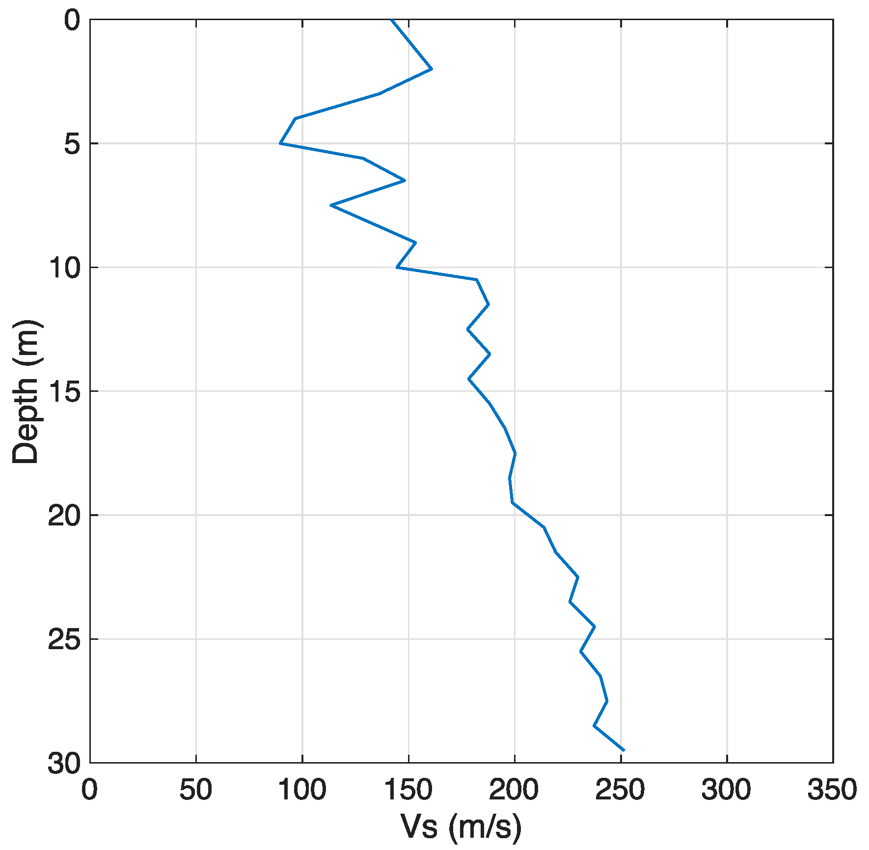
The second soil profile, called BOWW, was extracted from a set of six profiles considered within a recent SSI study by the authors [1]. It has a total thickness of 800 m. The VS profile and soil stratigraphy information, as well as a set of geomechanical parameters used to describe the dynamic soil behaviour in terms of the shear modulus reduction and damping curves, were extracted from the Groningen microzonation studies by Kruiver et al. (2017) [16] and Rodriguez-Marek et al. (2017) [17], to which interested readers are referred for details. The shear wave velocity profile, characterised by an average VS over the top 30 m, VS,30, equal to 174 m/s, is shown in Figure 5, while for the main stratigraphy and geotechnical properties interested readers are referred to the report by Mosayk (2020) [18].
2.3. Seismic Input
In site response analyses, the seismic input typically takes the form of an acceleration history applied at the bottom of the soil deposit. Two records were selected herein for the dynamic analyses accounting for kinematic soil-structure interaction. The first one, originally labelled “23G461”, was taken from a set of three relatively weak records considered in the Groningen study by the authors [1], which are all borehole recordings at a 50-m depth. Although it was already the strongest one of those three records, with a magnitude ML 3.1, an epicentral distance of 12 km and a peak ground acceleration (PGA) of 0.2 m/s2, it was here linearly scaled up by a factor of 3 so that the soil response could more easily be pushed into its nonlinear range. Figure 6 displays the acceleration histories and response spectra of the two horizontal components, namely H1 and H2, of this record, which will be henceforth referred to as “Accel borehole”.
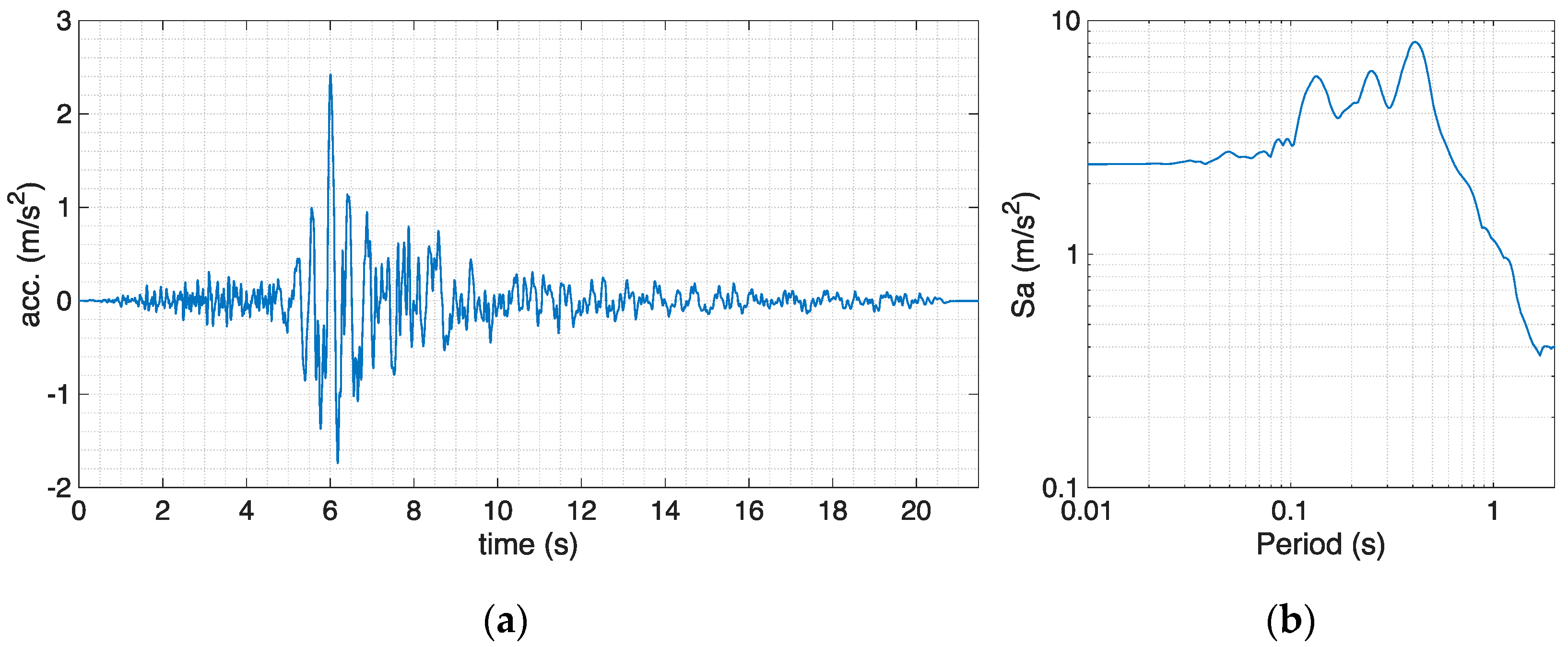
The second record that was selected belongs to the Central Italy earthquake sequence of 2016. It was extracted from the Italian Accelerometric Archive (ITACA) database [19] among the records of the first main event of the sequence (24 August 2016). With a magnitude ML 6.0, an epicentral distance of 33 km and a PGA equal to 2.42 m/s2 for the East-West horizontal component, it is the strongest one among the records available for that event on soil type A, which indicates rock or very stiff soil with VS higher than 800 m/s, according to the current Italian building code (NTC18) [20]. It was registered at the recording station with code name “FEMA”, and will hereafter be referred to as “Accel outcrop”. Figure 7 displays the acceleration history and response spectrum of the selected East-West component of record “Accel outcrop”. This component was used in both horizontal directions within the 3D soil-block analyses (see Section 4.2); however, this choice did not influence the results, since the response in only one horizontal direction is of interest here, as will be further discussed at the end of Section 3.1.
The definition of the seismic input to be introduced at the base of the soil-block model in OpenSees (see Section 3.1) required the undertaking of a preparatory step, different for each one of the two soil profiles.
For the academic soil profile, it was decided to only apply the “Accel outcrop” signal, recorded on rock outcrop, since record “Accel borehole”, having been recorded in a borehole of a Groningen soil profile, is characterised by features not consistent with the properties of the simple academic profile. A relatively limited depth of 30 m was adopted for the soil-block analyses, so as to decrease the computational burden and thus render this numerical exercise computationally feasible (see [1] for more details on the choice of this depth). The input signal for the soil-block model at a 30-m depth was taken from a convolution process carried out in DEEPSOIL [21], with the “Accel outcrop” record applied at the 100-m-deep bedrock (see [5] for additional information).
On the other hand, for the BOWW profile, both records were applied. The soil-block analyses were carried out for a depth of 30 m, as done for the first profile. The acceleration histories at a 30-m depth, for both records, were obtained by convolution using STRATA [22] (see [5] for additional information). Concerning the “Accel borehole” accelerogram, which was recorded at a 50-m-deep borehole station, both components were introduced in the STRATA model as “within” motions at a 50-m depth, whereas the “Accel outcrop” record was applied at the bedrock of the STRATA model, at an 800-m depth, as a rock outcrop motion. Then, for both records, the upward propagating motions that serve as input to the OpenSees model were extracted at a 30-m depth as outcrop motions.
3. Numerical Model of Soil and Structure
As already mentioned, the finite element site response analyses carried out in the present work aimed at capturing the kinematic soil-structure interaction effects due to a building’s basement, and at comparing the FE-based transfer functions derived from the results of such analyses with analytical counterparts available in the literature. A study of the structural response is therefore outside the scope of this paper and, consequently, the capability to capture nonlinear response was only assigned to the soil-block model, while the structural components were modelled using elastic elements.
3.1. 3D Nonlinear Numerical Model of Layered Soil
The 3D numerical model of layered soil developed by the authors [1], implemented in OpenSees and underlain by either an elastic or a rigid half-space, was used herein to represent the two soil profiles briefly introduced in Section 2.2. The base nodes of the soil-block model are fixed vertically. To ensure equal horizontal displacements, equalDOF boundary conditions are applied in the two horizontal directions (global x and z) to all nodes belonging to the soil-block’s edges and base. Eight-node SSPbrick elements compose the soil-block model. The soil layers can be assigned linear or nonlinear materials. In the nonlinear case, the elastic-plastic PressureIndependMultiYield material is adopted and shear modulus degradation curves can be assigned to all soil layers, considering their initial confinement pressure. The Poisson’s coefficient was set to 0.45, considering undrained conditions and numerical stability of the analyses.
In order to accurately reproduce the propagation of the shear waves below a frequency of interest, the soil-block mesh size should be such that at least eight elements are included within the minimum wavelength, λ, of the input seismic excitation; to this aim, a horizontal mesh size of 1 m was chosen in both x- and z-directions (i.e., 1 × 1 m2 square elements) for both soil profiles (see [1] for additional details). Along the vertical y-direction, layers thicker than 1 m were subdivided into two or more sublayers, so that the largest sublayer thickness is 1 m. The accuracy of these mesh settings was checked by model validation, comparing the output results with those obtained with other software packages (see [1,5]). As an example, Figure 8 displays the comparison between results obtained in OpenSees with the soil-block model reduced to a 50 × 1 × 1 m3 soil-column, DEEPSOIL (both nonlinear, NL, and equivalent linear, EL, solutions) and STRATA, for the BOWW soil profile and record “Accel borehole”, in terms of surface acceleration histories (limited to the initial four seconds of dynamic analysis to cater for a more immediate inspection of the match) and response spectra. As can be noted from Figure 8, the obtained match is very satisfactory, especially considering the markedly different modelling approaches adopted in the three programs, thus demonstrating the robustness of the developed soil-block model and the accuracy of the adopted mesh settings [5].
In the developed soil-block model, in order to attenuate numerical noise possibly present in the analyses, a Rayleigh damping formulation was adopted, requiring the selection of values for the damping ratio and two modal frequencies. The former was assigned the very low value of 1%, as already done in [1], whilst the latter were set to the first (fundamental) frequency of the deposit and five times that frequency, namely 1.43 Hz and 7.15 Hz for the BOWW profile and 1.25 Hz and 6.25 Hz for the academic profile. An estimation of the fundamental period, T1, was retrieved by the common expression:
where H is the total thickness of the soil deposit (i.e., 30 m for both soil profiles), while the average shear wave velocity, , is commonly obtained starting from the shear wave velocity values of the N layers within H, VS,i, and their thicknesses, di:
In order to reproduce the finite rigidity of the underlying elastic half-space, a compliant base with a quiet (absorbing) boundary was used at the base of the soil-block mesh. In particular, two Lysmer and Kuhlemeyer (1969) [23] viscous dashpots were attached independently at the base of the soil-block in the global x- and z-directions, thus introducing radiation damping. The OpenSees viscous uniaxial material was assigned to the zeroLength elements representing the dashpots. Following the method of Joyner and Chen (1975) [24], the dashpot coefficient, cb, is defined as the product of the mass density, ρb, and shear wave velocity, VS,b, of the underlying elastic layer, and the soil-block base area, A. Earthquake excitation is input to the system as two force histories, Fx(t) and Fz(t), in the two directions, applied at the dashpot free nodes and proportional through the dashpot constant to the two velocity time series, vx(t) and vz(t), at the model base.
Both force histories were applied at the base, thus carrying out full three-dimensional analyses. However, given the symmetric (square) properties of both soil-block and structure (for a description of the latter, see Section 3.2), all plots included in Section 4.2 are related to the same horizontal direction, namely the x-direction. In Figure 9, a rendering of the soil-block model for soil profile BOWW is shown.
3.2. 3D Numerical Model of Building with Basement
The model for the building with basement described in Section 2.1 was created in OpenSees according to the following modelling strategy.
Once the soil-block model had been created, it was necessary to remove several soil brick elements in the upper soil layers to model the excavation opening. Since the soil nodes previously belonging to the brick elements cannot be left free, and removing them would alter the complex node numbering in the soil-block or impact the recording settings in OpenSees, such nodes are linked by equalDOF constraints to one of the soil nodes in the model: the first node was chosen herein as the master node, but this choice does not have an impact on the model and results, since the equalDOF constraints are only applied to avoid numerical issues. Subsequently, the elastic square slab at the bottom of the excavation hole is modelled with the same SSPbrick elements used for soil, though obviously characterised by concrete material properties, having the same discretisation used for soil elements (i.e., 1 × 1 m2) and a thickness of 0.25 m.
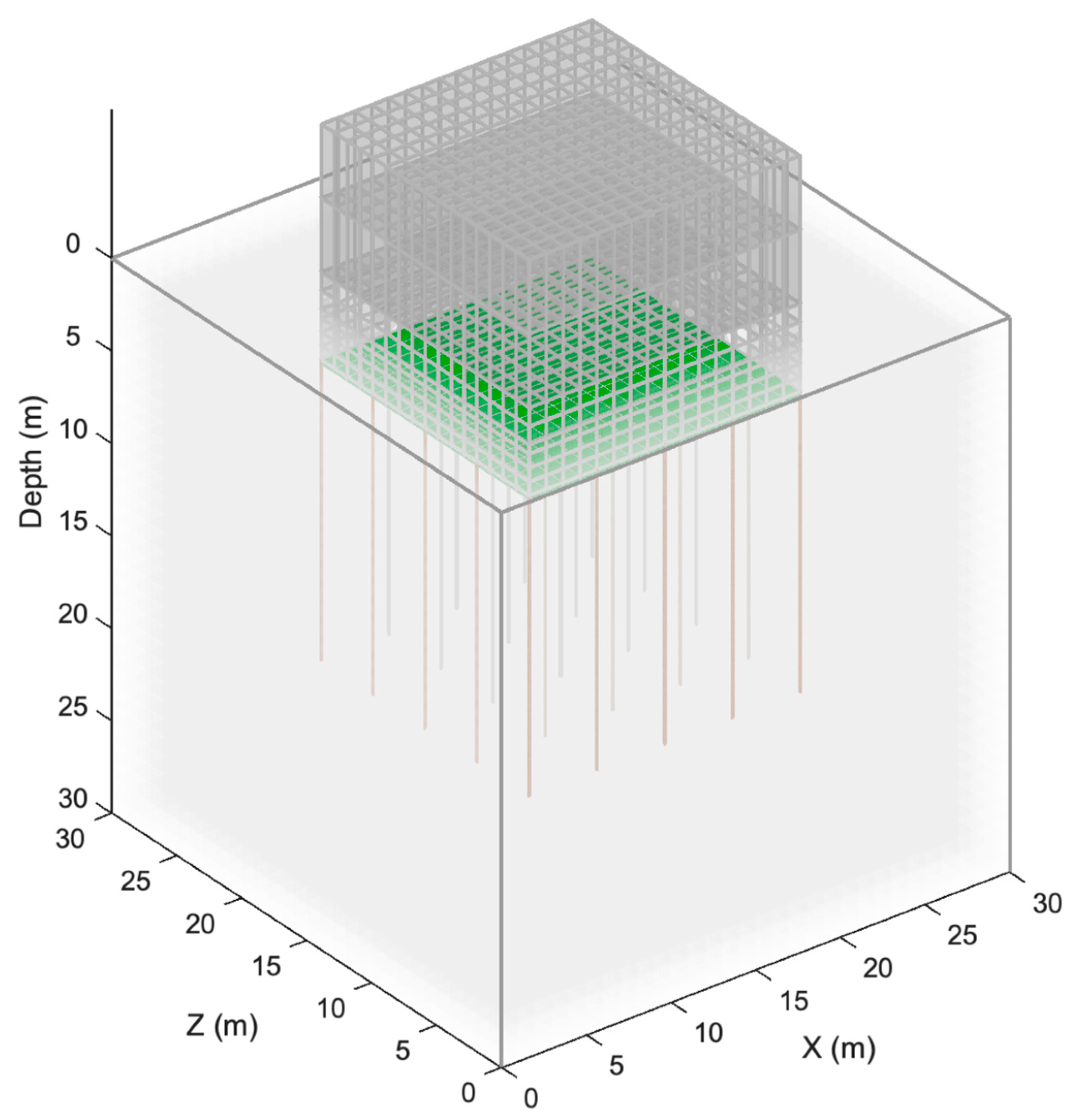
The superstructure is composed of four vertical panels, which represent the masonry walls, and three horizontal panels, representing the timber floor slabs and the roof. Shell elements of type ShellMITC4 are employed for the panels, with shell section of type ElasticMembranePlateSection to assign the structure an elastic behaviour. The base nodes of the vertical panels are linked to the base slab’s upper nodes by equalDOF constraints in all three directions. Soil constraints at the ground level are modelled by zeroLength elements characterised by an Elastic-Perfectly Plastic Gap material with zero gap size and negative force to introduce a compression gap. Elastic frame elements of type elasticBeamColumn are used to model the wooden piles, spaced by 4 m along both horizontal directions, for a total of 25 piles. Figure 10 shows the building with an embedded basement of 5-m depth founded on a 30 × 30 × 30 m3 soil-block, whereas Table 1 reports the adopted values for the most relevant properties of the building model. Since the aim of this study is to capture the kinematic SSI effects only, neglecting the inertial ones, the building’s total mass of 363 tonnes and the corresponding weight were disregarded in the structural model, and this is why mass properties of the used materials (i.e., concrete, masonry and timber) are missing in Table 1. Still, in order to properly capture the kinematic interaction effects, and differently from some of the past works discussed earlier, which introduced rigid elements within the excavation opening, herein the massless superstructure was modelled, so as to account for the actual stiffness of the vertical panels, floor slabs and roof, with their materials (masonry and timber).
Regarding the possible presence of scattered non-vertically propagating waves due to the absence of absorbing elements at the vertical sides of the mesh and the presence of the structure, it is noted that previous works by the authors [1,18] showed that (i) the adopted mesh size is appropriate for this building with basement and (ii) the model does not give rise to reflected waves at the vertical boundaries. Further details on this structural model and the choice of the soil-block size can be found in [1,18].
4. Transfer Functions for Embedment Effects
Transfer functions represent the ratio between two ground motions in the frequency domain. As such, these functions can be conveniently used to quantify the kinematic SSI effects, in terms of the variation of a ground motion at the foundation level of a structure with respect to the free-field. In the evaluation of transfer functions, signal processing may be needed, including windowing (to obtain the S-wave portion of the record) and smoothing (to attenuate scatter that can hide physically significant trends). However, it has been observed that while the transfer function ordinates can be locally affected by the window length and the degree of smoothing, the general shape and magnitude of the transfer functions are kept essentially unchanged [25]. For that reason, in this work, only a simple moving average (over a sliding window of 50 points) was applied to the numerically derived FE-based transfer functions, sufficient to readily allow comparisons between the latter and the analytical ones taken from the literature.
Transfer function models for embedment effects are commonly characterised by two different expressions, valid for the translational and rotational components of the foundation input motion (FIM), respectively. In this work, only the translational component of both FE-based and analytical transfer functions was considered, given that it is by far the most relevant one for typical earthquake engineering applications, such as the correction of motions recorded at the basement level of a building. Furthermore, the rotational component is not deemed to be relevant when the slenderness of the embedment, expressed as the ratio between the embedment depth and plan dimensions, is low, as is the case for the building considered herein.
Sotiriadis et al. (2020, 2019) [4,26] derived transfer functions from real recordings and compared them with those obtained from numerical analyses; in the latter, the substructure approach was undertaken and the FIM employed in dynamic single-degree-of-freedom (SDOF) analyses to account for the inertial interaction was obtained using the transfer function model for embedment effects proposed by Elsabee and Morray (1977) [11]. It is noted that the expression for translation in [11] is basically the same as the one found in the report by NIST (2012) [10]: the only difference is the meaning of shear wave velocity, which in [11] is the velocity along the embedment depth, whereas in [10] it is the average effective profile velocity (see Section 4.1). Along the lines of the work in [4,26], Zogh et al. (2021) [27] obtained recordings from two instrumented nuclear power plants in Japan with large footprints and embedment depths. The transfer functions from these recordings were then compared with those proposed by NIST (2012) [10], finding that the latter underestimate the FIM at higher frequencies. Another important work in the field, although not relevant for the scope of this paper and reported here only to render the review more comprehensive, is the study by Conti et al. (2018) [28], which aims at highlighting the effect of the foundation mass on the filtering action produced by embedded foundations. Since the foundation mass is explicitly included in the kinematic interaction, the involved interaction problem can be called “quasi-kinematic”. A new transfer function model for rigid massive embedded foundations was derived using a 2D finite difference soil-block model and 1D limit solutions.
Based on the literature review briefly outlined above, it was decided to check the validity of the translational components of only two transfer function models for embedment effects, namely the ones proposed by NIST (2012) [10] and Conti et al. (2017) [9], as stated already in Section 1.
4.1. Investigated Transfer Function Models
The first transfer function model for embedment effects investigated herein is the one proposed by NIST (2012) [10]. This model is the adaptation to rectangular foundation shapes of the analytical solutions by Kausel et al. (1978) [29] and Day (1978) [30], applicable to rigid cylinders embedded in a uniform soil of finite or infinite thickness (i.e., half-space). Given a building with weight W and equivalent plan dimensions B and L, the overburden stresses due to the building weight below the embedment depth, D, are determined assuming a 45° spanning of the soil stresses with depth z:
Note that this corresponds to a total stress increase which is equal to the corresponding effective stress increase. In fact, any increase in porewater pressure due to the building weight causes a potential flow of the excess porewater pressure that is assumed to have disappeared a few months after the construction of the building. The overburden-corrected shear wave velocities may then be determined assuming (i) a linear variation of the soil shear modulus with effective mean soil stress, i.e., n = 1 in Equation (4), (ii) a variation of the effective mean soil stress proportional to the vertical effective stress, i.e., constant earth pressure coefficient at rest, k0, and (iii) the fact that the shear wave velocity is proportional to the square root of the soil shear modulus, i.e., . The corrected shear wave velocity expression is then given by (NIST, 2012) [10]:
where is the effective vertical stress from the soil self-weight at depth z. For the purpose of the analysis of kinematic interaction effects, the average value of the shear wave velocity below the basement level may be computed on the basis of the travel-time of shear wave velocities within a depth equal to the half-dimension of an equivalent square foundation matching the area of the entire building footprint, i.e., (see the report by NIST, 2012 [10]). The average effective profile velocity thus becomes:
where nl is the number of layers in , each with thickness and overburden-corrected shear wave velocity VS,Fi. Note that the value should be rounded so as to correspond to the sum of thicknesses of the nl layers over which the average is calculated.
For embedded rectangular foundations, the NIST transfer function for horizontal foundation translation is expressed as a function of circular frequency ω, embedment depth D and average effective profile velocity VS,eff, defined in Equation (5):
An additional transfer function found in the report by NIST (2012) [10], aiming at correcting the base-slab averaging of incoherent incident waves, could actually have been considered for validation in this work. However, it was disregarded since the developed soil-block model produces vertically propagating plane shear waves; in this condition, incoherence is not present and base-slab averaging cannot occur, with filtering effect being only related to the inability of the embedded foundation to follow soil deformations induced by travelling waves [9].
The second transfer function model investigated in this work, proposed by Conti et al. (2017) [9], is more refined than the first one, since it includes, in addition, the dependence on B/D, in which B is the width of the square foundation. The proposed expression for the translational component is given by:
where the dependence on the ratio B/D is present in the coefficients a1, a2 and a3, whose expressions are reported in [9]. For consistency with the model by NIST (2012) [10], the same definition for VS, namely the average effective profile velocity VS,eff, was used in Equation (7). From the case study results, it was also observed that averaging VS,F values over D or (D + ), in place of , leads to negligible variations of VS,eff and, as a consequence, of both analytical transfer functions.
4.2. FE-Based Transfer Functions and Comparison with Analytical Ones
In this section, the numerical FE-based transfer functions obtained from the soil-block analyses are compared with those derived from analytical models proposed by NIST (2012) [10] and Conti et al. (2017) [9].
Starting with the case of homogeneous academic soil profile with linear material subjected to record “Accel outcrop”, Figure 11 shows the surface free-field motion and signals at the basement level at the two considered depths of 2.5 m and 5 m, in terms of acceleration histories and response spectra. Computing the ratio between the amplitude of the Fourier transforms of the signals at the basement level and of the free-field surface motion yields the transfer functions displayed in green in Figure 12. First, it can be noticed that the two investigated analytical models lead to transfer functions that are similar and diverge at lower periods only. The numerical/analytical match can be deemed to be satisfactory, with small divergences appearing at lower periods (or higher frequencies) only. The mismatch is more pronounced for the larger embedment depth of 5 m, especially within a small period range between 0.1 and 0.2 s. At higher periods, the models correctly predict a constant transfer function value equal to 1, the same obtained from the soil-block analyses, as also gathered from the response spectra comparison in Figure 11b. Based on these observations, it can be concluded that both models are able to reliably predict the embedment effects in this “ideal” case. The obtained good match serves both purposes of (i) proving the applicability of analytical models in “ideal” conditions and (ii) confirming once again (after the validation in [5]) that the developed soil-block model is robust and produces reliable results.
It is noted that the transfer functions shown in Figure 12 and the subsequent figures are plotted and compared up to a period of 0.07 s because the soil-block model, with the adopted maximum mesh size of 1 m in the vertical direction, is able to accurately capture a range of frequency up to around 15 Hz; the latter value is obtained considering an average VS of around 150 m/s and a λ/10 ratio for the mesh size, which leads to a minimum wavelength, λ, equal to 10 m. Limiting the upper frequency for comparison is also consistent with the findings of Kim and Stewart (2003) [31].
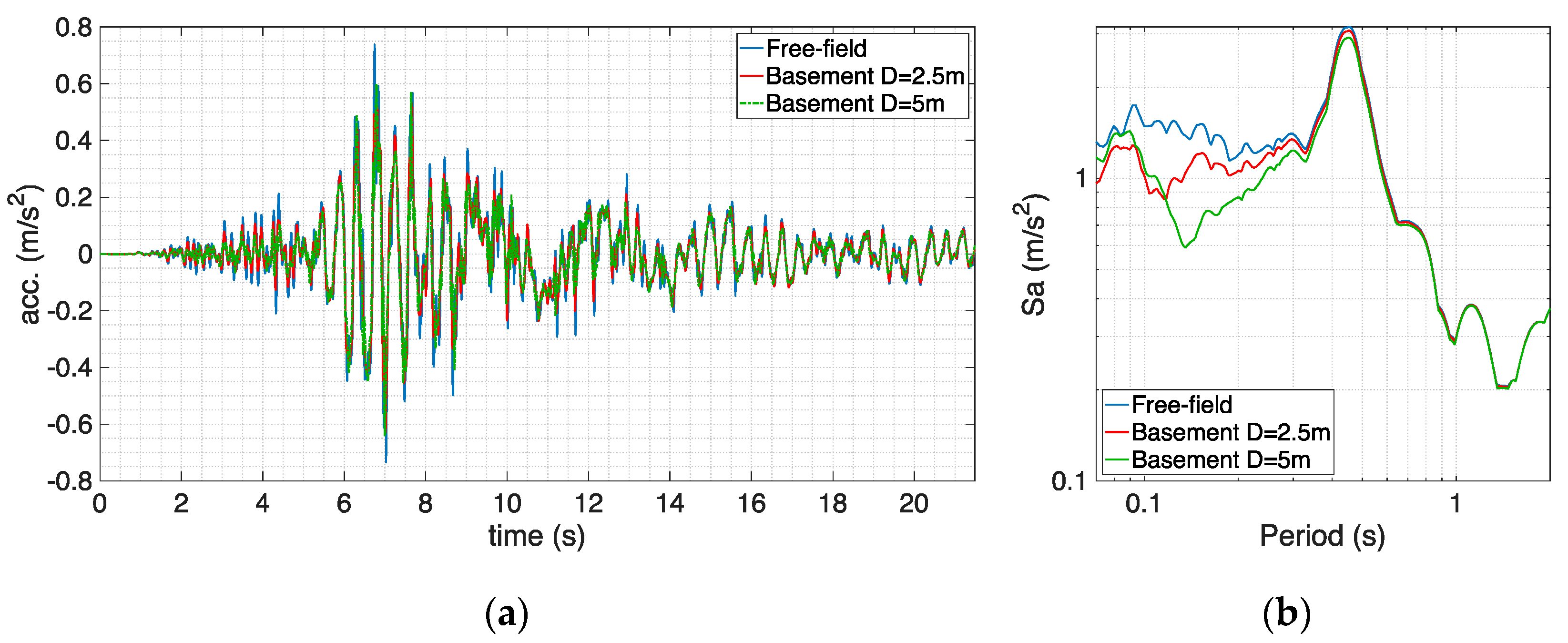
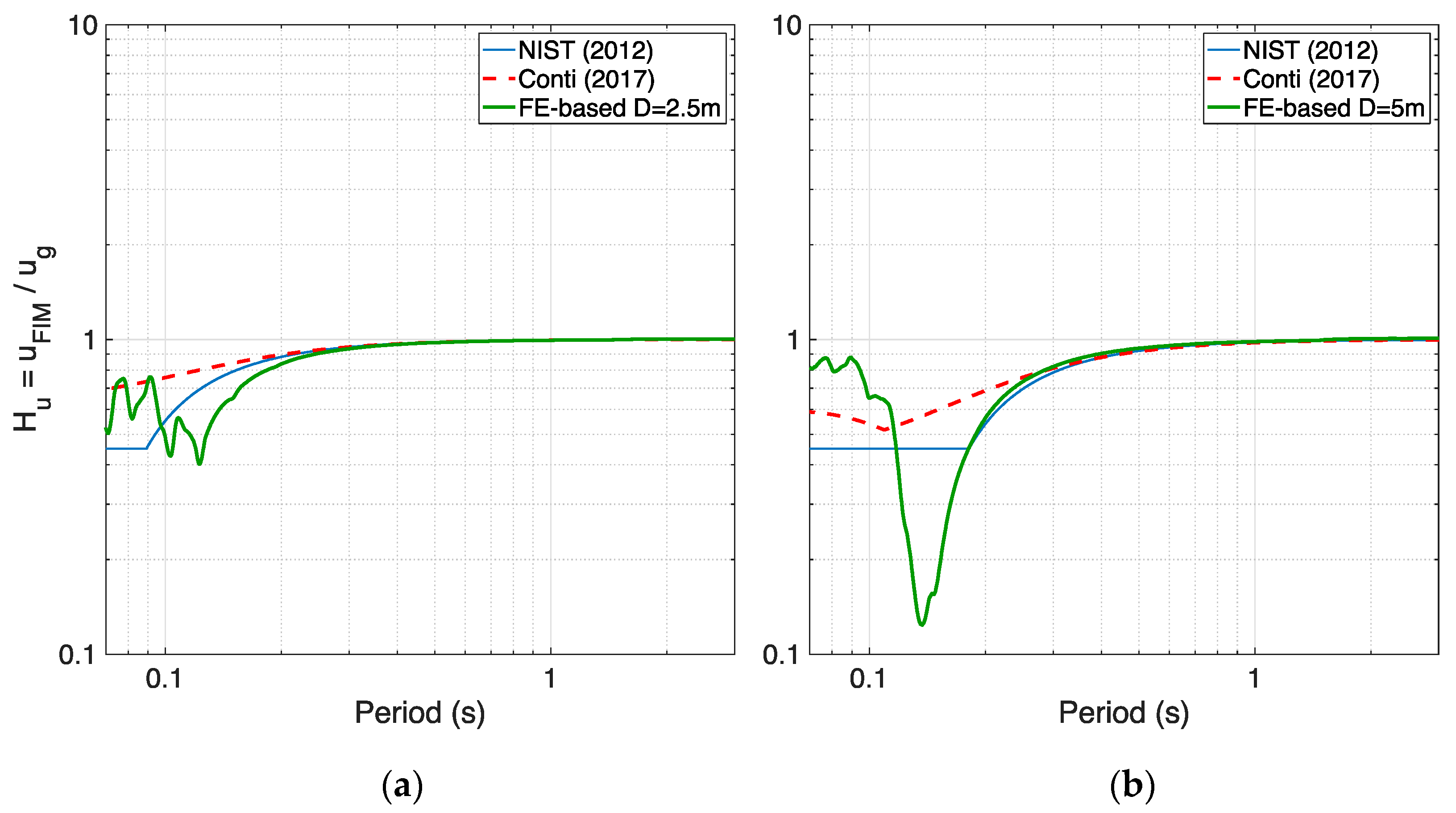
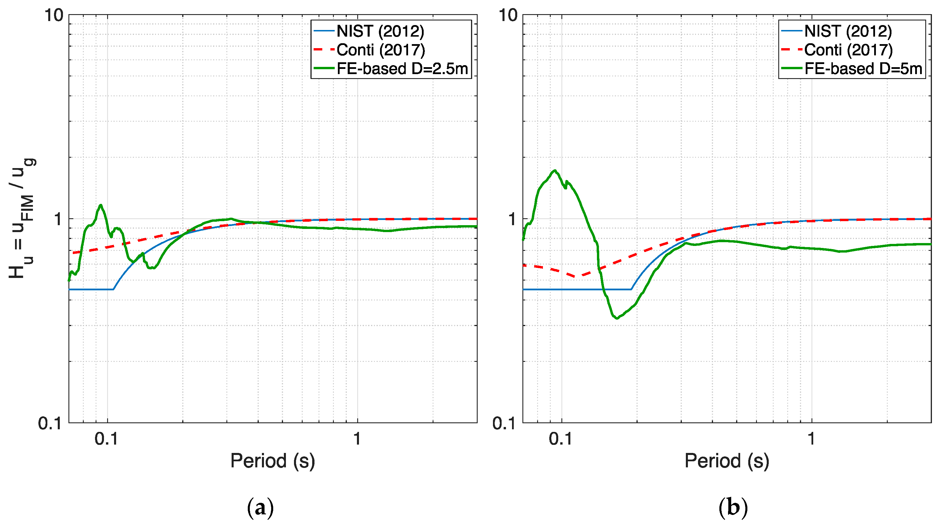
In case the same academic profile is assigned nonlinear soil properties, with a low value for VS and de-amplification of shear waves (as reported in [5]), the free-field and foundation-level motions feature a smaller PGA due to energy dissipation in the nonlinear range, as shown in Figure 13. The deviation of the numerical transfer functions from the analytical ones, displayed in Figure 14, is basically the same as the one observed for the linear case, for both embedment depths, with a more relevant mismatch, limited again to lower periods, appearing for the larger embedment depth of 5 m.
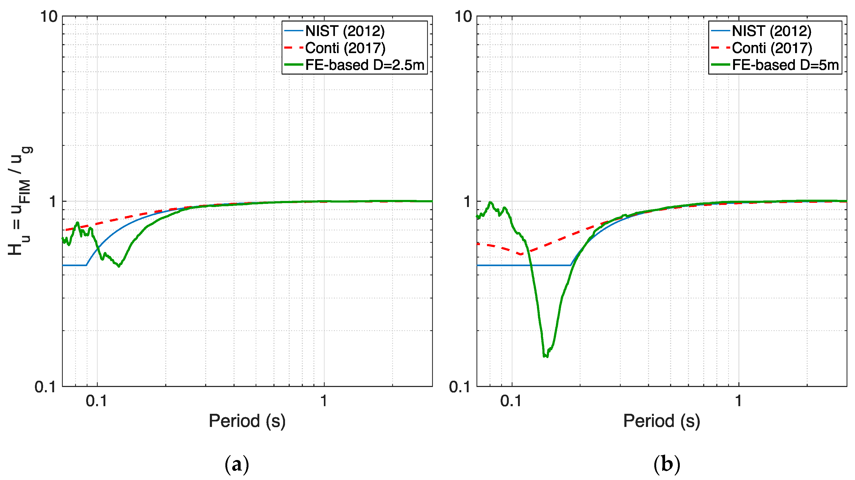
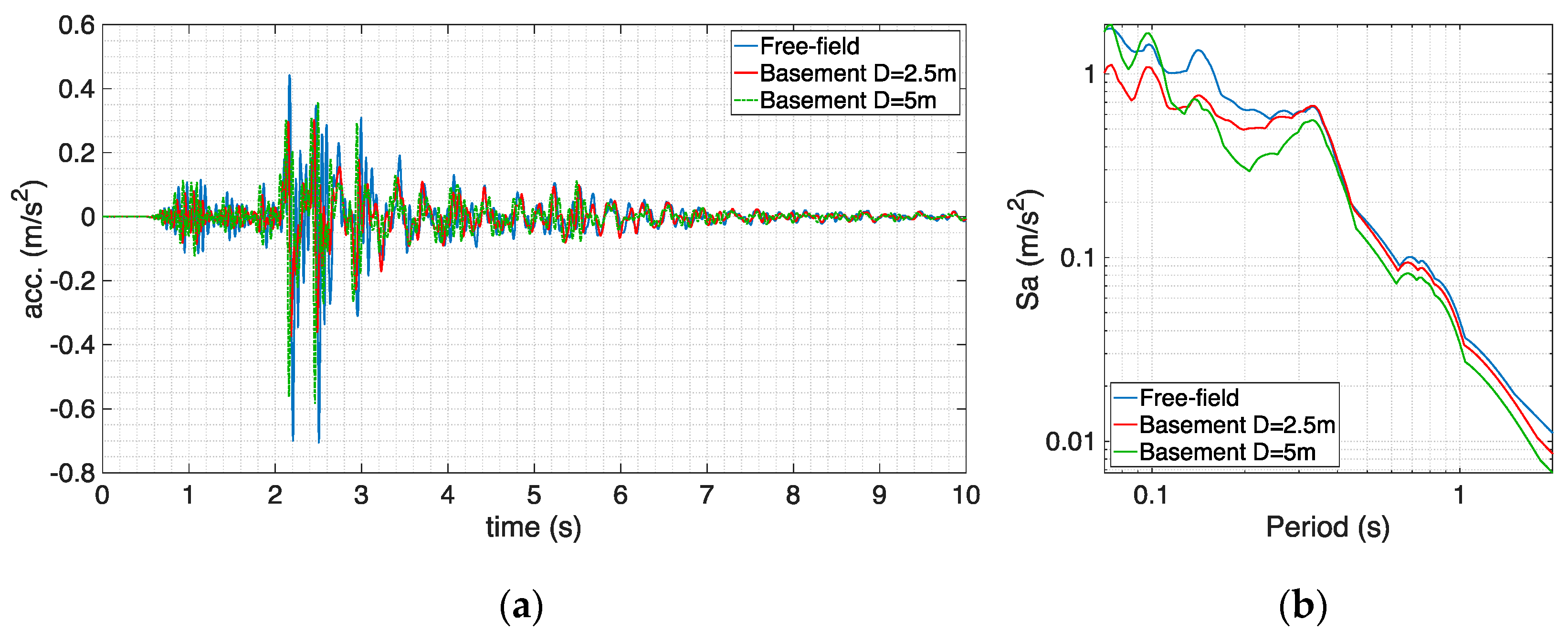
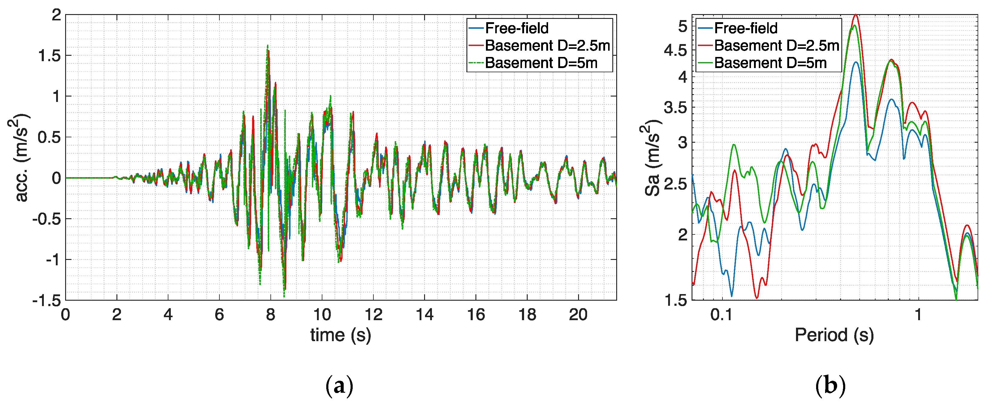
Moving to the non-homogeneous nonlinear soil profile, herein called BOWW, subjected to record “Accel borehole”, the free-field and foundation-level motions are shown in Figure 15. Even if the soil experiences only light nonlinearity under this less intense record, the divergences between the obtained transfer functions are now spread out over the entire period range, not only at lower periods, as readily gathered from Figure 16. The numerical/analytical match can be still considered acceptable only for the smaller embedment depth of 2.5 m, whereas the deviations observed for the larger embedment depth of 5 m are more pronounced and may have been exacerbated by an abrupt reduction of shear wave velocity at a 5-m depth (see Figure 5), something that can indeed occur in real soil profiles such as the BOWW profile adopted in this study.
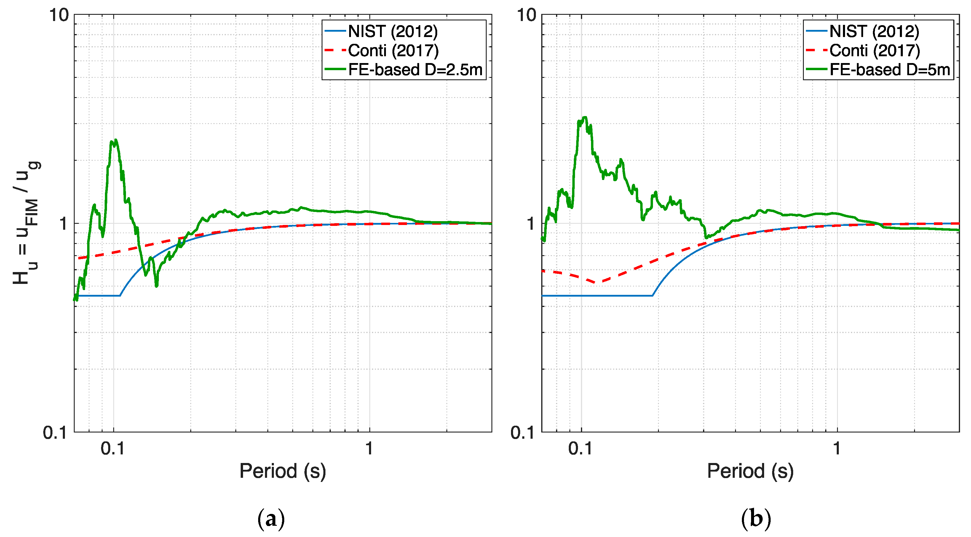
Finally, when the stronger record “Accel outcrop” is input at the base of the BOWW profile (obtained motions displayed in Figure 17) and the soil experiences a higher level of nonlinearity, the most significant numerical/analytical deviations are observed, as expected, once again especially for the larger embedment depth of 5 m, as shown in Figure 18. In summary, the comparisons reported in Figure 16 and Figure 18, as well as the spectra plots in Figure 15b and Figure 17b, all related to the BOWW profile, show that contrarily to what is predicted by analytical models, the motion at the basement level of a building can be more intense than the free-field one, and this can happen especially at lower periods and for larger embedment depths. It is recalled that such an observation of frequency-dependent foundation motion amplified with respect to the free-field one is also reported in the work by Sotiriadis et al. (2020, 2019) [4,26] and NIST (2012) [10].
5. Conclusions
While SSI effects are typically neglected for relatively lightweight and short buildings resting on shallow foundations, large heavy buildings feature a foundation-level motion that may significantly deviate from the free-field one. Focussing in particular on the perturbation of the free-field motion caused by the presence of a basement, this paper attempted to assess the applicability of analytical transfer function models for embedment effects. This was carried out by means of comparisons of results given by the latter and those obtained with a 3D nonlinear soil-block model representing a layered soil, recently developed and validated by the authors [1,5], and featuring on top a large heavy building with a basement.
The comparisons seemed to show that analytical transfer function models are able to reliably predict the embedment effects only when a homogeneous “academic” soil profile with linear or nonlinear material is considered. Regarding the non-homogeneous nonlinear soil profile, an acceptable numerical/analytical match was observed only for the smaller embedment depth of 2.5 m under the less intense record, namely “Accel borehole”, for which the soil experiences light nonlinearity. On the other hand, significant deviations are observed when the stronger “Accel outcrop” was employed or, in general, for the larger embedment depth of 5 m. The presented results suggest that the performance of the investigated analytical models worsens as the considered soil/input conditions move away from idealised ones, and may thus not be satisfactory in real conditions, namely when a non-homogeneous profile with nonlinear behaviour under a given seismic excitation is considered, especially in presence of a deep basement (i.e., more than one storey high). Divergences between numerical and analytical transfer functions may also be partly due to the rigid foundation assumption under which analytical models are developed, whereas a real foundation, as modelled in this study, may be very stiff but not exactly rigid.
The above conclusions were drawn by considering a limited number of cases, in terms of seismic input signals, soil profiles and embedment depths of the building’s basement. This limitation was decided with a view to make this study computationally feasible, given the quite heavy numerical burden of the 3D soil-block finite element analyses undertaken herein: owing to the complexity of the numerical model, which includes thousands of 3D brick elements, each single site response analysis in OpenSees has taken about four weeks to complete, on dedicated numerical servers. Collection of a larger sample of numerical data may be needed to make more refined predictions on the applicability of analytical transfer function models available in the current literature. Nonetheless, it is believed that the results of this study do shed additional light on the influence of SSI on the recordings from instruments located at the basement of buildings and do highlight the need for judicious care when employing analytical models for correction of basement records used in the framework of ground motion models development and/or seismic hazard assessment.
Author Contributions
Conceptualization, F.C., A.A.C. and R.P.; methodology, F.C., A.A.C. and R.P.; software, F.C.; validation, F.C., A.A.C. and R.P.; formal analysis, F.C.; investigation, F.C., A.A.C. and R.P.; resources, F.C., A.A.C. and R.P.; data curation, F.C.; writing—original draft preparation, F.C.; writing—review and editing, F.C., A.A.C. and R.P.; visualization, F.C.; supervision, R.P.; project administration, R.P. All authors have read and agreed to the published version of the manuscript.
Funding
This research received no external funding.
Acknowledgments
The authors are very appreciative of the constructive feedback of two anonymous reviewers, which undoubtedly led to the improvement of the original version of the manuscript.
Conflicts of Interest
The authors declare no conflict of interest.
References
- Cavalieri, F.; Correia, A.A.; Pinho, R. Variations between foundation-level recordings and free-field earthquake ground mo-tions: Numerical study at soft-soil sites. Soil Dyn. Earthq. Eng. 2021, 141, 106511. [Google Scholar] [CrossRef]
- Mylonakis, G.; Nikolaou, S.; Gazetas, G. Footings under seismic loading: Analysis and design issues with emphasis on bridge foundations. Soil Dyn. Earthq. Eng. 2006, 26, 824–853. [Google Scholar] [CrossRef]
- Varghese, R.; Boominathan, A.; Banerjee, S. Investigation of pile-induced filtering of seismic ground motion considering em-bedment effect. Earthq. Eng. Struct. Dyn. 2021, 50, 3201–3219. [Google Scholar] [CrossRef]
- Sotiriadis, D.; Klimis, N.; Margaris, B.; Sextos, A. Analytical expressions relating free-field and foundation ground motions in buildings with basement, considering soil-structure interaction. Eng. Struct. 2020, 216, 110757. [Google Scholar] [CrossRef]
- Cavalieri, F.; Correia, A.A.; Pinho, R. Comparative nonlinear SSI analyses using macro-element and soil-block modelling ap-proaches. Submitted for publication. Bull. Earthq. Eng. 2021. [Google Scholar]
- Echebba, E.; Boubel, H.; El Omari, A.; Rougui, M.; Chourak, M.; Chehade, F. Analysis of the Second Order Effect of the SSI on the Building during a Seismic Load. Infrastructures 2021, 6, 20. [Google Scholar] [CrossRef]
- Karatzetzou, A.; Pitilakis, D. Modification of Dynamic Foundation Response Due to Soil-Structure Interaction. J. Earthq. Eng. 2018, 22, 861–880. [Google Scholar] [CrossRef]
- Karatzetzou, A.; Pitilakis, D. Reduction factors to evaluate acceleration demand of soil-foundation-structure systems. Soil Dyn. Earthq. Eng. 2018, 109, 199–208. [Google Scholar] [CrossRef]
- Conti, R.; Morigi, M.; Viggiani, G.M.B. Filtering effect induced by rigid massless embedded foundations. Bull. Earthq. Eng. 2017, 15, 1019–1035. [Google Scholar] [CrossRef] [Green Version]
- NIST. Soil-Structure Interaction for Building Structures; Report No. 12-917-21; National Institute of Standards and Technology: Gaithersburg, MD, USA, 2012. [Google Scholar]
- Elsabee, F.; Morray, J.P. Dynamic Behavior of Embedded Foundations; Report No. R77-33; Massachusetts Institute of Technology: Cambridge, MA, USA, 1977. [Google Scholar]
- McKenna, F.; Fenves, G.L.; Scott, M.H. OpenSees: Open System for Earthquake Engineering Simulation; University of California: Berkeley, CA, USA, 2000; Available online: http://opensees.berkeley.edu (accessed on 10 September 2021).
- Arup. External RVS Inspection Full Report Hoofdstraat-West 1, Uithuizen—Groningen Earthquakes—Structural Upgrading; Report no 9981AA_001_000_BE_REP_001; Version 6.3; Arup: London, UK, 2015. [Google Scholar]
- Witteveen+Bos. Dynamic Amplification Effects for B-Stations Due to Building Response; Report 113982/19–1009.783; Witteveen+Bos: Deventer, The Netherlands, 2019. [Google Scholar]
- Darendeli, M.B. Development of a New Family of Normalized Modulus Reduction and Material Damping Curves. Ph.D. Thesis, University of Texas, Austin, TX, USA, 2001. [Google Scholar]
- Kruiver, P.P.; Van Dedem, E.; Romijn, R.; De Lange, G.; Korff, M.; Stafleu, J.; Gunnink, J.L.; Rodriguez-Marek, A.; Bommer, J.; Van Elk, J.; et al. An integrated shear-wave velocity model for the Groningen gas field, The Netherlands. Bull. Earthq. Eng. 2017, 15, 3555–3580. [Google Scholar] [CrossRef] [Green Version]
- Rodriguez-Marek, A.; Kruiver, P.P.; Meijers, P.; Bommer, J.; Dost, B.; Van Elk, J.; Doornhof, D. A Regional Site-Response Model for the Groningen Gas Field. Bull. Seism. Soc. Am. 2017, 107, 2067–2077. [Google Scholar] [CrossRef]
- Mosayk. Soil-Structure-Interaction Analysis in Support of Groningen B-Stations Verification Efforts; Report No. D16; Mosayk: Pavia, Italy, 2020; Available online: http://www.nam.nl/feiten-en-cijfers/onderzoeksrapporten.html (accessed on 10 September 2021).
- D’Amico, M.; Felicetta, C.; Russo, E.; Sgobba, S.; Lanzano, G.; Pacor, F.; Luzi, L. Italian Accelerometric Archive v3.1; Istituto Nazionale di Geofisica e Vulcanologia, Dipartimento della Protezione Civile Nazionale: Rome, Italy, 2020; Available online: http://itaca.mi.ingv.it/ItacaNet_31/#/home (accessed on 10 September 2021).
- NTC18. Aggiornamento delle “Norme tecniche per le costruzioni”. In Decreto Ministeriale del 17/01/2018. Suppl. ord. n. 8 alla G.U. n. 42 del 20/02/2018 (in Italian); Ministero delle Infrastrutture e dei Trasporti: Rome, Italy, 2018. [Google Scholar]
- Hashash, Y.M.A.; Musgrove, M.I.; Harmon, J.A.; Ilhan, O.; Xing, G.; Numanoglu, O.; Groholski, D.R.; Phillips, C.A.; Park, D. DEEPSOIL 7.0, User Manual; Board of Trustees of University of Illinois at Urbana-Champaign: Urbana, IL, USA, 2020. [Google Scholar]
- Kottke, A.R.; Rathje, E.M. Technical Manual for Strata; Report No. 2008/10; Pacific Earthquake Engineering Research Center, University of California: Berkeley, CA, USA, 2008. [Google Scholar]
- Lysmer, J.; Kuhlemeyer, R.L. Finite Dynamic Model for Infinite Media. J. Eng. Mech. Div. 1969, 95, 859–878. [Google Scholar] [CrossRef]
- Joyner, W.B.; Chen, A.T. Calculation of nonlinear ground response in earthquakes. Bull. Seismol. Soc. Am. 1975, 65, 1315–1336. [Google Scholar]
- Mikami, A.; Stewart, J.P.; Kamiyama, M. Effect of time series analysis protocols on transfer functions calculated from earth-quake accelerograms. Soil Dyn. Earthq. Eng. 2008, 28, 695–706. [Google Scholar] [CrossRef]
- Sotiriadis, D.; Klimis, N.; Margaris, B.; Sextos, A. Influence of structure–foundation–soil interaction on ground motions rec-orded within buildings. Bull. Earthq. Eng. 2019, 17, 5867–5895. [Google Scholar] [CrossRef]
- Zogh, P.; Motamed, R.; Ryan, K. Empirical evaluation of kinematic soil-structure interaction effects in structures with large footprints and embedment depths. Soil Dyn. Earthq. Eng. 2021, 149, 106893. [Google Scholar] [CrossRef]
- Conti, R.; Morigi, M.; Rovithis, E.; Theodoulidis, N.; Karakostas, C. Filtering action of embedded massive foundations: New analytical expressions and evidence from 2 instrumented buildings. Earthq. Eng. Struct. Dyn. 2018, 47, 1229–1249. [Google Scholar] [CrossRef]
- Kausel, E.; Whitman, A.; Murray, J.; Elsabee, F. The spring method for embedded foundations. Nucl. Eng. Des. 1978, 48, 377–392. [Google Scholar] [CrossRef]
- Day, S.M. Seismic response of embedded foundations. In Proceedings of the ASCE Convention and Exposition, Chicago, IL, USA, 18–21 June 1978; American Society of Civil Engineers: New York, NY, USA, 1978. [Google Scholar]
- Kim, S.; Stewart, J.P. Kinematic Soil-Structure Interaction from Strong Motion Recordings. J. Geotech. Geoenviron. Eng. 2003, 129, 323–335. [Google Scholar] [CrossRef]
Figure 1.
Building with basement case study (Arup, 2015) [13].
Figure 1.
Building with basement case study (Arup, 2015) [13].

Figure 2.
Building with basement case study: structural drawing (Witteveen+Bos, 2019) [14] of the portion selected for this study.
Figure 2.
Building with basement case study: structural drawing (Witteveen+Bos, 2019) [14] of the portion selected for this study.

Figure 3.
Scheme and basic properties of the academic soil profile.

Figure 4.
(a) Modulus reduction and (b) damping curves for the different layers of the academic soil profile.
Figure 4.
(a) Modulus reduction and (b) damping curves for the different layers of the academic soil profile.

Figure 5.
Shear wave velocity profile for the BOWW soil profile.

Figure 6.
Horizontal components of record “Accel borehole” (already scaled by a factor of 3) in terms of acceleration (a) histories and (b) response spectra.
Figure 6.
Horizontal components of record “Accel borehole” (already scaled by a factor of 3) in terms of acceleration (a) histories and (b) response spectra.

Figure 7.
East-West horizontal component of record “Accel outcrop” (Central Italy) in terms of acceleration (a) history and (b) response spectrum.
Figure 7.
East-West horizontal component of record “Accel outcrop” (Central Italy) in terms of acceleration (a) history and (b) response spectrum.

Figure 8.
Comparison between results obtained in OpenSees (soil-block model), DEEPSOIL (NL and EL solutions) and STRATA for a 50-m-deep soil column for the BOWW soil profile and record “Accel borehole”, in terms of surface acceleration (a) histories and (b) response spectra.
Figure 8.
Comparison between results obtained in OpenSees (soil-block model), DEEPSOIL (NL and EL solutions) and STRATA for a 50-m-deep soil column for the BOWW soil profile and record “Accel borehole”, in terms of surface acceleration (a) histories and (b) response spectra.

Figure 9.
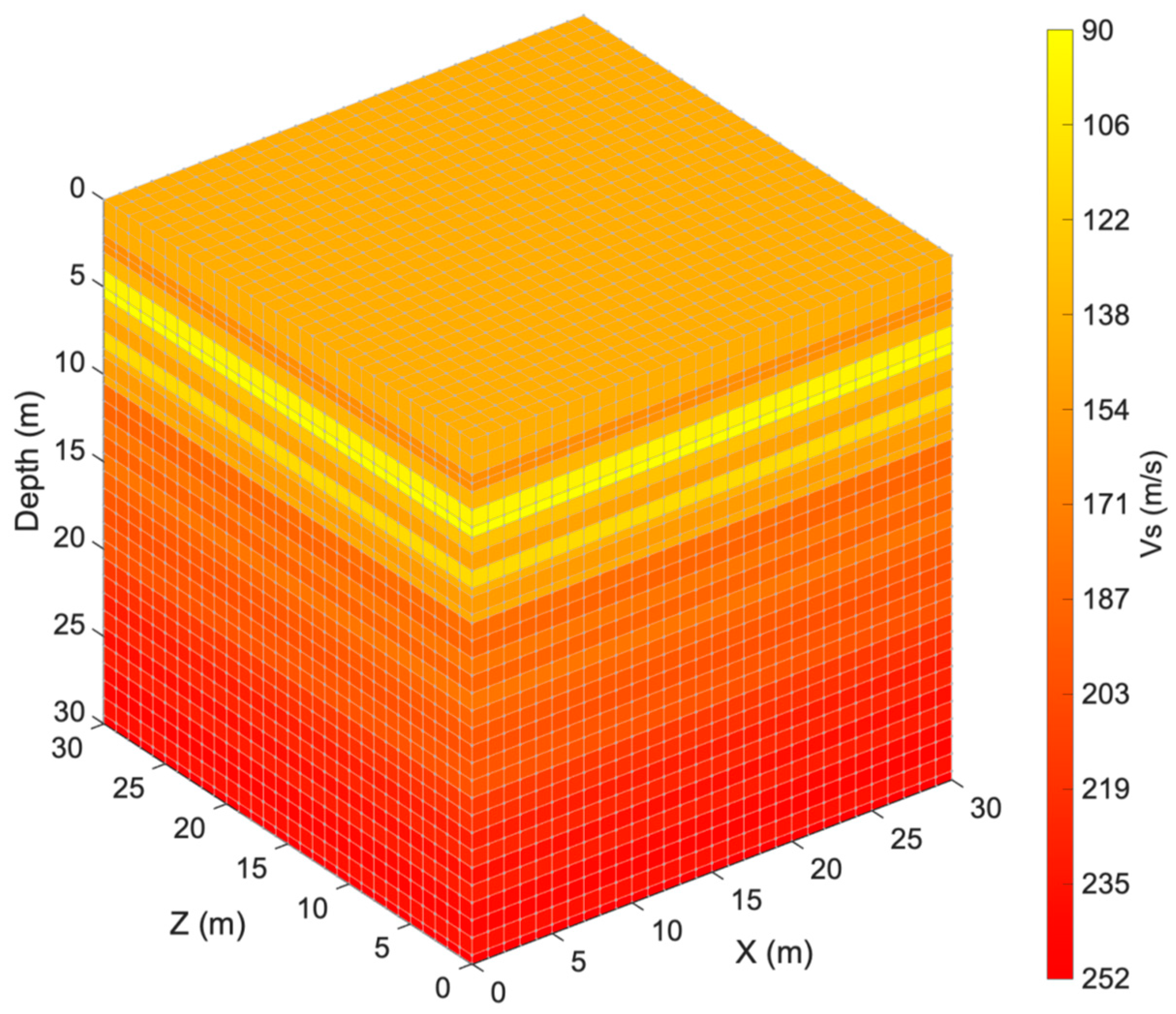
Developed soil-block model for the BOWW soil profile, with size 30 × 30 × 30 m3.

Figure 10.
Soil-block with a 16 × 16 m2 building with basement (of 5-m depth) on top. The soil, wall and roof panel elements are rendered in transparent fashion, so as to allow visualisation of the concrete base slab, represented in green colour, as well as of the timber piles, represented in brown colour.

Figure 11.
Comparison between surface free-field motion and signals at basement level (two different depths) for linear academic soil profile and record “Accel outcrop” in terms of acceleration (a) histories and (b) response spectra.
Figure 11.
Comparison between surface free-field motion and signals at basement level (two different depths) for linear academic soil profile and record “Accel outcrop” in terms of acceleration (a) histories and (b) response spectra.

Figure 12.
Comparison between analytical transfer functions obtained from two models and finite element-based (FE-based) ones for embedment depths of (a) 2.5 m and (b) 5 m for linear academic soil profile and record “Accel outcrop”.
Figure 12.
Comparison between analytical transfer functions obtained from two models and finite element-based (FE-based) ones for embedment depths of (a) 2.5 m and (b) 5 m for linear academic soil profile and record “Accel outcrop”.

Figure 13.
Comparison between surface free-field motion and signals at basement level (two different depths) for nonlinear academic soil profile and record “Accel outcrop” in terms of acceleration (a) histories and (b) response spectra.
Figure 13.
Comparison between surface free-field motion and signals at basement level (two different depths) for nonlinear academic soil profile and record “Accel outcrop” in terms of acceleration (a) histories and (b) response spectra.

Figure 14.
Comparison between analytical transfer functions obtained from two models and FE-based ones for embedment depths of (a) 2.5 m and (b) 5 m for nonlinear academic soil profile and record “Accel outcrop”.
Figure 14.
Comparison between analytical transfer functions obtained from two models and FE-based ones for embedment depths of (a) 2.5 m and (b) 5 m for nonlinear academic soil profile and record “Accel outcrop”.

Figure 15.
Comparison between surface free-field motion and signals at basement level (two different depths) for BOWW soil profile and record “Accel borehole” in terms of acceleration (a) histories and (b) response spectra.
Figure 15.
Comparison between surface free-field motion and signals at basement level (two different depths) for BOWW soil profile and record “Accel borehole” in terms of acceleration (a) histories and (b) response spectra.

Figure 16.
Comparison between analytical transfer functions obtained from two models and FE-based ones for embedment depths of (a) 2.5 m and (b) 5 m for BOWW soil profile and record “Accel borehole”.
Figure 16.
Comparison between analytical transfer functions obtained from two models and FE-based ones for embedment depths of (a) 2.5 m and (b) 5 m for BOWW soil profile and record “Accel borehole”.

Figure 17.
Comparison between surface free-field motion and signals at basement level (two different depths) for BOWW soil profile and record “Accel outcrop” in terms of acceleration (a) histories and (b) response spectra.
Figure 17.
Comparison between surface free-field motion and signals at basement level (two different depths) for BOWW soil profile and record “Accel outcrop” in terms of acceleration (a) histories and (b) response spectra.

Figure 18.
Comparison between analytical transfer functions obtained from two models and FE-based ones for embedment depths of (a) 2.5 m and (b) 5 m for BOWW soil profile and record “Accel outcrop”.
Figure 18.
Comparison between analytical transfer functions obtained from two models and FE-based ones for embedment depths of (a) 2.5 m and (b) 5 m for BOWW soil profile and record “Accel outcrop”.


Table 1.
Properties of the building with basement structural model (c: concrete, m: masonry, t: timber).
Table 1.
Properties of the building with basement structural model (c: concrete, m: masonry, t: timber).
| Base dimens. (m) | Height of superstr. (m) | Depth of basement (m) | Ec (kPa) | νc | Thickn. of base slab (m) | Em (kPa) | νm |
| 16.0 × 16.0 | 8.0 | 2.5 m or 5.0 m | 3.0 × 10⁷ | 0.3 | 0.25 | 9.0 × 10⁶ | 0.2 |
| Thickness of walls (m) | Et (kPa) | νt | Thickn. of floor slabs/roof (m) | Pile diameter (m) | Pile length (m) | Pile spacing along x (m) | Pile spacing along z (m) |
| 0.22 | 1.1 × 10⁷ | 0.2 | 0.2 | 0.35 | 16.0 | 4.0 | 4.0 |
Publisher’s Note: MDPI stays neutral with regard to jurisdictional claims in published maps and institutional affiliations. |
© 2021 by the authors. Licensee MDPI, Basel, Switzerland. This article is an open access article distributed under the terms and conditions of the Creative Commons Attribution (CC BY) license (https://creativecommons.org/licenses/by/4.0/).
Share and Cite
MDPI and ACS Style
Cavalieri, F.; Correia, A.A.; Pinho, R. On the Applicability of Transfer Function Models for SSI Embedment Effects. Infrastructures 2021, 6, 137. https://doi.org/10.3390/infrastructures6100137
AMA Style
Cavalieri F, Correia AA, Pinho R. On the Applicability of Transfer Function Models for SSI Embedment Effects. Infrastructures. 2021; 6(10):137. https://doi.org/10.3390/infrastructures6100137
Chicago/Turabian StyleCavalieri, Francesco, António A. Correia, and Rui Pinho. 2021. "On the Applicability of Transfer Function Models for SSI Embedment Effects" Infrastructures 6, no. 10: 137. https://doi.org/10.3390/infrastructures6100137