On the Dynamic Capacity of Concrete Dams


1
Mott MacDonald, Croydon CR0 2EE, UK
2
Department of Civil Engineering, University of Colorado, Boulder, CO 80309, USA
3
X-Elastica, LLC, Boulder, CO 80303, USA
4
Ricerca Sistema Energetico (RSE), 20134 Milan, Italy
*
Author to whom correspondence should be addressed.
Infrastructures 2019, 4(3), 57; https://doi.org/10.3390/infrastructures4030057
Submission received: 28 June 2019
/
Revised: 21 August 2019
/
Accepted: 27 August 2019
/
Published: 31 August 2019
(This article belongs to the Special Issue Advances in Dam Engineering)
Abstract
:The purpose of this joint contribution is to study the maximum dynamic load concrete dams can withstand. The so-called “dynamic capacity functions” for these infrastructures seems now technically and commercially feasible thanks to the modern finite element techniques, hardware capabilities, and positive experiences collected so far. The key topics faced during the dynamic assessment of dams are also discussed using different point of view and examples, which include: the selection of dynamic parameters, the progressive level of detail for the numerical simulations, the implementation of nonlinear behaviors, and the concept of the service and collapse limit states. The approaches adopted by local institutions and engineers on the subject of dam capacity functions are discussed using the authors’ experiences, and an overview of time and resources is outlined to help decision makers. Three different concrete dam types (i.e., gravity, buttress, and arch) are used as case studies with different complexities. Finally, the paper is wrapped up with a list of suggestions for analysts, the procedure limitations, and future research needs.
1. Introduction
This paper is an extended and modified version of the contribution presented during the “3rd Meeting of EWG Dams and Earthquakes”, which was held May 2019 in Lisbon, Portugal [1]. While the skeleton of the presentation was kept, many new references, literature review, simulations, and discussion were added to the paper.
Special efforts have been devoted in recent years to the dynamic assessment of large dams. High seismicity countries went through (or are still facing) re-assessment programs for their dams [2,3,4,5]. These extensive studies are required for the lack of seismic checks on older dams, updated seismic hazard parameters, and new seismic standards [6]. Despite the opportunities offered by modern technologies, it is sometimes difficult to select a cost-effective (yet high-confidence) procedure for the seismic assessment of dams. It is understandable that complex analyses make stakeholders feel uncomfortable making risk-related decisions. For this reason, in the authors’ opinion, it is vital to find new procedures to balance the numerical simulations with comprehensible outcomes (i.e., the capacity curves’ appreciation is easier than the judgment of stress map outputs qualitatively).
The seismic analyses of large dams must consider the following features [7,8]: specific seismic hazard assessment [9,10,11], step-by-step analysis approach [12], soil-structure interaction [13], fluid–structure interaction [14], and the system’s nonlinear behavior [15,16]. It is a common opinion that concrete dams (especially arch dams) are unique prototypes, each having their own behavior. Even more so, it is generally expected that the seismic response of the concrete dams should be considered with an opportune degree of distinction between different case studies. Previous experiences on the application of capacity functions [17,18] demonstrated that using certain classification rules, the overall seismic behavior of concrete dams may be similar, especially towards the failure point. This aspect should exhort the scientific community and the best practice of the sector to consider capacity functions as a way forward.
While the precise time history analysis for concrete dams with dam-specific ground motion records has been the subject of much research, this paper provides a framework to estimate the capacity of dams with a novel technique. Therefore, the objective is not to validate a numerical procedure, but to provide the best estimate of the nonlinear seismic response at different shaking intensities, as well as the failure capacity. This will be accomplished using some examples showing the advantages and limitations of this approach. A summary of conventional procedures available to extract the capacity functions is also discussed. Special attention is offered to the Endurance Time Analysis (ETA) method [19]. Finally, a technical discussion is presented on the benefits that capacity functions can add to the dam industry and public interests.
1.1. International Experiences in the Seismic Assessment of Dams
Following a period in which the lack of regulations permitted designing and building dams without or with too simplified seismic design principles, the necessity to cope with the safety reassessment of these dams and to select the right method to evaluate their performance during the earthquake event is now well recognized. Despite the variety of seismic safety approaches in dam engineering, the concept of “risk assessment” is, implicitly or explicitly, present in all technical codes used in most of the developed countries, e.g., [2,3,4,5].
In Switzerland, which recently has undertaken the task of re-assessing the dams [20], some outlines are provided on the framework and efforts required to manage the dams’ portfolios, referring to their risk classification. After 10 years required to assess 208 dams, important outcomes and lessons learned have been collected by the Swiss experience. It is worth noting that the cases appeared to be non-compliant with the standards where generally dams had problems primarily in static conditions or unusual design concepts. According to OFEG [21], a lower occurrence probability should be expected for earthquakes, when the failure consequences are very high at the downstream. However, it does not provide any indication on the earthquake level leading to dam failure.
Other European countries followed the example of Switzerland for seismic assessment of their dams. For instance, recently adopted dam safety regulations introduced risk concepts such as the residual safety margin of the dam against seismic actions, a kind of qualitative evaluation of the dam’s capacity. Despite this, it is still necessary to bridge the gap between the seismic response determined for the target seismic levels, mainly collapse and serviceability Limit States (LSs), and the dams’ ultimate capacity. Considering this, it appears clear where the so-called “capacity functions” may play their role.
The proposed engineering guide for seismic risk of dams in the U.K. guidelines is based on the dam category and has three main features [22]: the probability of occurrence of an earthquake larger than the Maximum Scenario Earthquake (MSE), the vulnerability of the dam, and the consequences of the failure. The French guide [23] is mainly focused on gravity dams. It covers the fundamental stability analysis for sliding LS with a focus on material strength. There is no new recommendation concerning seismic loads [24]. Similar experiences can be found in other countries such as India [25], Japan [26], and Turkey [27].
1.2. An Overview of Seismic Assessment Procedures
To evaluate what may be called the “failure” or “critical earthquake” of a concrete dam, it is necessary to put in place a numerical model and a seismic assessment procedure to consider the most important aspects involved. Considering recent advancements in computer science, the idea to investigate the nonlinear behavior of concrete dams towards collapse is becoming more common among researchers and engineers. Despite the excellent work done or planned in the future, the greatest obstacle for nonlinear analysis and capacity functions is the formal definition of acceptable damages against the different LSs used in the modern structural codes. At the current stage, we can simulate the structural performance decay of these structures, but we have no practical guidelines to indicate if their expected behavior is acceptable other than subjective engineering judgment.
In the buildings sector, the capacity functions are used to demonstrate that the design target and the actual structural ductility are met [28,29]. A similar route can be expected for dams, with appropriate procedures for the definition of “failure modes” and “limit states”. An important aspect to be considered is the confidence with the methods used to produce the capacity functions. In the buildings sector, the use of nonlinear static pushover analysis is considered common practice [30]. Pre-defined load patterns are used to reproduce the effects produced by earthquakes. This loading pattern is then increased through a scale factor to produce the damages of the main structural elements until the point of collapse. Based on the authors’ experience, it is not possible to use the same procedure for dams. This is due to the different way the dam and the surrounding domains, foundation and water, react against the seismic actions. For this reason, it is more reasonable to use a bespoke dams sector approach. This may consist of nonlinear dynamic analysis procedures where all the mechanism involved in the response can be included and properly captured without limits associated with standardized pseudo-static forces (pre-defined load pattern shapes increased monotonically).
A capacity function determined for a concrete dam under dynamic/seismic forces is always associated with concurrent actions, namely dead weight, thermal loading, and hydrostatic pressure, applied to the dam before the seismic excitation. In addition, the seismic actions are characterized by their spatial variation using three directions of the seismic action and concurrency factors. The numerosity of the combinations suggests that capacity functions cannot be developed for all of them. A procedure is then necessary to perform a screening of the most critical combinations. The proposed approach is to start with simplified linear pseudo-static procedures, move to linear dynamic analysis, and finally nonlinear dynamic analysis. This approach is also giving assurance on the validity of the analysis methods while more detailed aspects are introduced, a concept already introduced within technical guidelines. In this case, the capacity function represents the last step of a series of analyses that are code compliant.
Developing a capacity function requires that the numerical model is capable of accounting for the main nonlinearities in the dam-foundation-reservoir system during an earthquake. For gravity dams, the sliding at the base, or at the weaker lift joints, is one of the main failure modes expected [31]. This phenomenon can cut off the seismic excitation acting as a seismic isolator. The reduction of stresses above the sliding plane is obtained at the cost of a residual displacement, captured by jumps in the force-displacement diagrams. Slips occurring over the joint are also important for arch dams, but are not governing the global response of these structures. On the other hand, the right representation of joint openings and closures are essential for arch dams to represent the different behaviors of these dams under seismic actions in different directions [32,33].
In addition, according to ICOLD [34], a large portion of the concrete dam failures can be attributed to foundation issues (either geological or geotechnical). Whereas dams have generic potential failure modes, foundation failure modes are very specific [35]. Depending on the initiator (i.e., static, hydrologic, or seismic), there might be different failure modes for the foundation. These kinds of geotechnical problems are not included in this paper, but must be considered for seismic assessments of dams. It is reasonable to think that capacity functions evaluated without considering the effects of foundation failure modes must be interpreted in conjunction with the geotechnical results.
For both gravity and arch dams, cracking behavior is required to consider the effects produced by the reduction of concrete properties along the dam body and the associated changes in the way the dam deforms. These effects are represented by the slope change in the capacity function. The nonlinear model used should be also selected based on the data necessary to evaluate damages and the associated relationship with LSs [36].
Another aspect to be considered for large models is the management of computation time as already mentioned. This depends highly on modeling techniques and assumptions. If a numerical model is considered in its most effective condition (mesh and time steps are key aspects in this sense), the only way to reduce the computational time required for the analysis is the selection of alternative seismic inputs. Among the dynamic analysis techniques, the ETA is one of the most efficient methods that significantly reduces the computational cost [17,18].
2. Capacity Estimation Techniques
In this section, a summary of the procedures available for the dynamic capacity estimation of concrete dams is given. The “dynamic capacity function” is defined as the relationship between an external parameter affecting the capacity of the structure (also referred to as a “stressor”), and the “response” of the system at the macro (or structural) level [37]. The stressor, S, can be: (1) an incrementally-increasing monotonic, cyclic (pseudo-dynamic, quasi-dynamic, or dynamic), or time-dependent load (or displacement, acceleration, pressure); (2) an incrementally-decreasing resistance parameter or degradation in strength properties; or (3) a discrete increasing/decreasing critical parameter in a system leading to failure. In earthquake engineering, the stressor is typically called an intensity measurement (IM) parameter [38].
The response, R, on the other hand, is representative of the system behavior under the varying stressor. It is depicted in either an absolute or relative sense. R may be: (1) a single damage variable (DV), such as drift or energy dissipation; (2) a combination of several DVs in terms of the damage index (DI); or (3) any safety monitoring index. In the field of earthquake engineering, R is typically called an engineering demand parameter (EDP) [39]. In the field of uncertainty quantification, it is called the quantity of interest (QoI) [40]. Several dam-specific EDPs, DVs, and DIs can be found in Zhang et al. [41], Hariri-Ardebili and Saouma [42], Ansari and Agarwal [43], and Hariri-Ardebili et al. [44].
2.1. Incremental Dynamic Analysis
Incremental dynamic analysis (IDA) is a technique to estimate the seismic capacity of dams using a large set of ground motions. IDA can be decomposed into the following major branches [37]:
- Single-record IDA (SR-IDA) vs. multi-record IDA (MR-IDA)
- Single-intensity IDA (SI-IDA) vs. multi-intensity IDA (MI-IDA)
- Single-EDP IDA (SE-IDA) vs. multi-EDP IDA (ME-IDA)
Any of these IDA types might be combined together. SR-IDA is the most basic technique, in which a single record is used for nonlinear time history analysis of a dam. Let be the “as-recorded” (unscaled) ground motion time history. To consider both the stronger and weaker scenarios, it can be scaled uniformly using a scale factor, . The scaled ground motion can be written as . This should be represented by a monotonic scalable IM (e.g., peak ground acceleration (PGA), or the 5% damped spectral acceleration at the first-mode period ()). Several nonlinear analyses are then performed with the scaled ground motions. Let us assume that the response of the nonlinear system to the scaled record is . The response parameter (or EDP or QoI) can be deformation, stress, uplift, or DI.
MR-IDA is a collection of n SR-IDA for the same structural system. The required ground motion records are usually obtained from a probabilistic seismic hazard analysis (PSHA) conducted for the dam site. The number of required records typically varies given the dispersion among them and the code requirements. The order of n for framed structures is about 30–50, while for concrete dams (which are computationally expensive), it is around 12–20.
SI-IDA uses only one intensity measure parameter (e.g., PGA) to characterize the ground motion record-to-record (RTR) variability; however, MI-IDA adopts additional intensity measure parameters to enhance the uncertainty quantification and to reduce the dispersion. On the other hand, SE-IDA uses only one EDP value (e.g., relative drift), while ME-IDA accounts for the joints’ EDPs (e.g., joint opening and sliding).
The combined multi-record single-intensity IDA (MR-SI-IDA) is the most common form of the IDA curves adopted by many researchers for different structures [45]. It is an IDA plot in the IM-EDP coordinate system. Figure 1 presents concrete dam-specific IDA curves developed by different researchers under various assumptions. Considering the RTR variability in the IDA capacity functions, they should be summarized using some central values like the mean, median, and 16% and 84% fractiles.
Therefore, different IDA versions come from different interpretations: MR-IDA is a multi-record of SR-IDA. Each of those two can be presented based on (a) single intensity (SI), or multi-intensity (MI), and/or (b) single EDP (SE), or multi EDP (ME). The simplest combination will be SR-SI-SE-IDA (i.e., single-record, single-intensity, single-EDP), which is just a curve in 2D space. The most complex one will be MR-MI-ME-IDA (i.e., multi-record, multi-intensity, multi-EDP), which consists of n curves in space (where m and p are the numbers of IMs and EDPs, respectively).
2.2. Cloud Analysis
In cloud analysis (CLA) (as opposed to IDA), the dam is subjected to a set of unscaled (or as-recorded) ground motions and analyzed numerically. If the ground motion records are extracted from a specific hazard scenario, they can be represented by (), i.e., the magnitude and distance representative of the bin. Therefore, the first n records are selected (or generated [53]). Then, they are applied to the finite element model, and subsequently, n linear or nonlinear transient simulations are performed. From these analyses, EDP vs. IM is determined and forms the so-called cloud response. The CLA method is usually used in the context of the probabilistic seismic demand model (PSDM) [54]. If the CLA is performed with a linear elastic model, the data points will have a linear trend in the arithmetic scale. Figure 2a shows the crest displacement vs. PGA of a tall gravity dam with linear elastic materials using about 2000 different ground motion records all based on a single seismic scenario. Although the results are based on linear analysis, a considerable dispersion exists at higher PGA levels. On the other hand, it is well accepted that the discrete data points resulting from nonlinear CLA have a linear trend on the logarithmic scale (Figure 2b), implying a power curve on the arithmetic scale. This figure shows the nonlinear response of another gravity dam with only 150 ground motions from six different seismic scenarios (i.e., S1–S6). As seen, the general trend is quite linear.
2.3. Endurance Time Analysis
Endurance time analysis (ETA) is a dynamic pushover procedure used to estimate the seismic performance of structures when subjected to pre-designed intensifying excitation [55,56]. The simulated acceleration functions are intended to shake the structure from a low excitation level (with a structural response in the elastic range) to a medium excitation level (where the structure experiences some nonlinearity) and ultimately to a high excitation level causing failure [57]. All these response ranges are experienced in a single time history analysis.
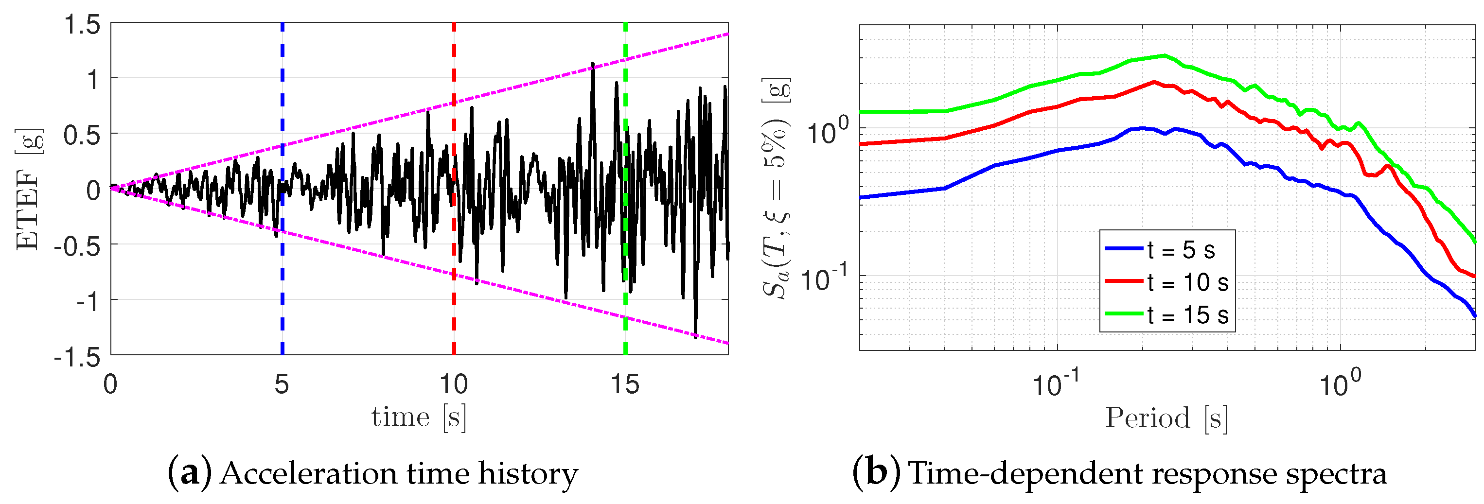
The challenging part of this method lies in generating the endurance time excitation functions (ETEFs), Figure 3a. Initial generation of ETEFs were only based on acceleration and displacement response spectra [58], while the recent advances in the simulation of ETEFs can be found in Mashayekhi and Estekanchi [59], and Mashayekhi et al. [60,61,62], where the functions were optimized in the time and frequency domains accounting for the acceleration and displacement response spectra, as well as the nonlinear displacement, absorbed hysteretic energy, number of effective cycles, etc. Unconstrained nonlinear optimization is used to simulate ETEFs. The objective function of simulating ETEFs problems is to compute differences between the dynamic characteristics of ETEFs and their intended target values. The objective function covers a range of pre-defined times, periods, and ductility ratios.
The ETEF is an artificially-designed intensifying acceleration time history, where the response spectra of the ETEF linearly increases with time; see Figure 3b. Ideally, the profile of the acceleration time history and response spectrum increase linearly with time. Figure 3 shows a sample ETEF and its response spectra at three different times (i.e., 5, 10, and 15 s). Note that the ETA and associated spectra are always evaluated from t = 0. Therefore, a particular time refers to time window . As seen, the spectrum at t = 10 s is nearly twice the one at t = 5 s, and the spectrum one at t = 15 s is three-times the one at t = 5 s. In this technique, the seismic performance is determined by the duration the structure can endure the dynamic input with increasing input intensity (i.e., acceleration). The longer the structure can endure the imposed stressor, the better the performance is. This is why it is named “endurance time analysis”.
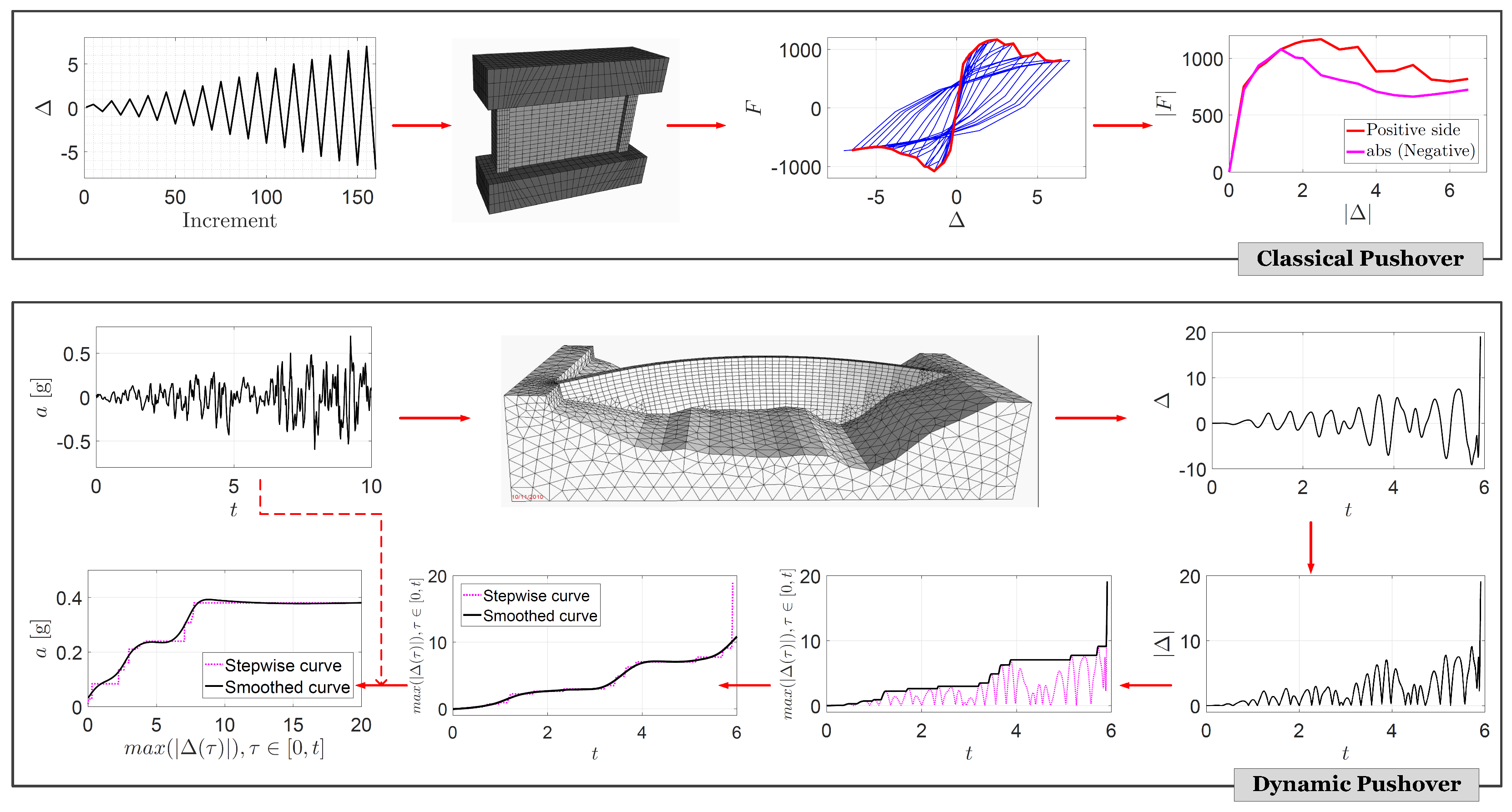
Figure 4 compares the cyclic pushover and the dynamic pushover (i.e., ETA) methods. In the cyclic pushover method, an increasing cyclic load or displacement function is applied to the finite element model, and the corresponding cyclic force-displacement plot is derived (note that this is different from monotonic pushover analysis in which the load/displacement is applied only in one direction) [63,64]. Next, the envelope of this hysteretic curve is computed (both in positive and negative directions), which forms the so-called capacity function. The applied load/displacement has a static or quasi-dynamic nature. Rate-dependent characteristics are not usually considered. On the other hand, a dynamic pushover method applies a time-dependent load/displacement and directly incorporates the material’s dynamic behavior. A capacity function in the ETA method can be obtained as:
- Develop the finite element model of the dam, and apply an appropriate ETEF.
- Record the time history of any desired EDP (or QoI), e.g., crest displacement in the horizontal direction. In nonlinear models, the analysis fails at some time, (e.g., = 5.9 s in Figure 4). Failure is interpreted either as a numerical non-convergence or physical failure (drift beyond a displacement threshold).
- Compute the absolute value of EDP at time interval . This step guarantees that all the peak values in positive and negative sides are incorporated in the final capacity function.
- Compute the maximum value of the absolute EDP at for any time interval using . The product of this step is a step-wise increasing function.
- Since the ETEFs have a stochastic nature, it is recommended to smooth them for any practical purposes. The resulting curve is called the ETA curve and is in the EDP-time coordinate system.
- Finally, the EDP-time coordinate system is flipped to make it time-EDP. Moreover, using the relationship between time and acceleration (from the original ETEF), one can convert the time parameter to its equivalent IM parameter. The final product will be a smoothed (or step-wise) curve in the IM-EDP coordinate system, which is the capacity function.
- Although this procedure is applicable only with a single ETEF, in order to reduce the uncertainty (due to the random nature of initial white noise in ETEF generation), the mean of three ETEFs typically is recommended.
3. Case Study Examples
According to the historical records collected by the ICOLD [66] (through its committee meetings and publications), concrete dams performed relatively well during earthquakes. The U.S. Committee on Large Dams published three comprehensive reports on the observed performance of dams during earthquakes [67,68,69]. In addition, Nuss et al. [70] collected a list of concrete dams that have been shaken by large earthquakes, but showed a relatively acceptable performance. Later, Hariri-Ardebili and Nuss [8] evaluated the seismic risk of these dams using a semi-quantitative approach and coupled it with finite element analyses. From previous experiences, the key role of the geometry on the seismic resistance of dams has been confirmed. For gravity dams, the use of narrowing sections at the neck is generally associated with cracking problems (e.g., Koyna dam [71,72]), while for the arch dams, a large “U” shape of the valley rift can affect negatively the overall seismic resistance of the dam [73]. These typical aspects of dams’ seismic vulnerability have been confirmed by post-earthquake inspections and structural analysis. Some examples of capacity functions are reported below. The finite element simulations have not been discussed in detail deliberately, allowing the readers to focus on the concept behind the use of capacity functions.
Three case studies are considered in this paper based on their complexities:
- Gravity dam: This is a 2D model of a gravity dam including the foundation and reservoir interactions. This example explains the progressive collapse in dams.
- Buttress dam: This is a single monolith of a buttress dam without a foundation and an empty reservoir. This simple example shows the impact of material uncertainties and also introduces the aspects associated with 3D blocks.
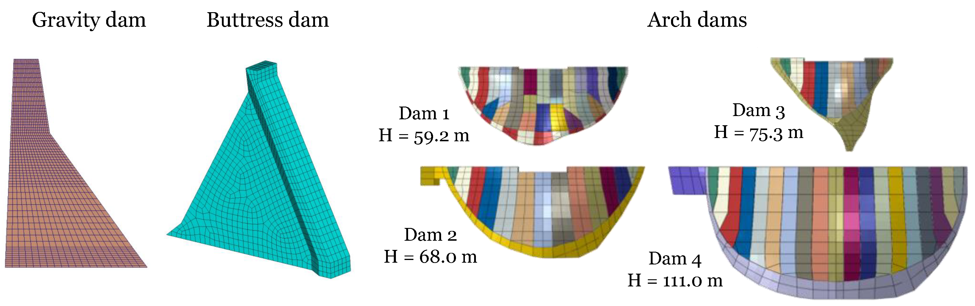
- Arch dams: This is a full nonlinear analysis of several arch dam-foundation-reservoir systems. It includes four dams presenting a portfolio of dams.
3.1. Gravity Dam
Koyna gravity dam has a 103-m height; the thicknesses at the base and at the crest are 70.2 m and 14.8 m, respectively, for the central non-overflow monoliths; see Figure 5. The mesh was refined around the neck and dam-foundation interface to capture all the potential failure modes precisely. The fluid–structure interaction (FSI) was applied according to the pressure-based fluid elements. The massless foundation was used, which might lead to slightly different response distribution in dams, particularly for relatively soft rocks, because the radiation damping is ignored. Applied loads on the system were: dam’s self-weight, hydrostatic pressure, bottom sediment, and seismic loads. Nonlinearity was originated from a concrete smeared crack model. The modulus of elasticity and compressive strength for concrete were assumed to be 26.4 GPa and 20.4 MPa, respectively. The modulus of elasticity of the foundation was 17 GPa.
3.2. Buttress Dam
Sefidrud buttress dam has a 106-m height in the middle section and consists of 26 monoliths, each 14 m long. The slopes of the dam on the downstream and upstream faces are 1:0.6 and 1:0.4, respectively [74]. It was constructed of plain concrete. It was assumed that the dam was fixed at the base where the ETEFs were applied. Figure 5 shows the finite element mesh. A 3D co-axial rotating smeared crack model was used for the nonlinear analyses [75]. The model was capable of cracking in three orthogonal directions, as well as crushing.
3.3. Arch Dams
Four arch dams were considered in this paper to introduce the key aspects associated with their seismic response towards global failure. Together they represent a reasonable representation of concrete arch dams with heights ranging from 59–111 m [17]; see Figure 5. For each dam, the interaction with the foundation was considered using the massless approach, which for high-intensity level earthquakes represents a major limitation (as discussed later in the paper). The FSI was accounted for by direct modeling the fluid domain using acoustic elements, a non-reflecting boundary condition at the far-end domain, and a wave reflection coefficient at the reservoir bottom. The nonlinear behavior of vertical and horizontal joints separating the different blocks of the dam were modeled to reproduce both joint slips and openings. The nonlinear behavior of concrete was considered using the damage plasticity model by Lee and Fenves [16]. Applied loads were: dead weight, hydrostatic load (full reservoir), winter thermal condition, and seismic loads. The water pressure inside the contraction joints was not modeled [76].
4. Results
4.1. Progressive Collapse of a Gravity Dam
The damage response of the case study gravity dam is explained in this section subjected to a fifteen-second ETEF. Figure 6a shows the variation of the normalized crest horizontal displacement with respect to the total dam height (i.e., 103 m). The dam showed a nearly linear displacement up to a PGA of 0.6 g with = 0.1. The first large normalized displacement jump occurred for a PGA of about 0.78 g (which corresponds to about 12 s of ETEF). Moreover, the variation of three cracks and the crushing is shown in Figure 6b using the concept of DI. Although many DIs have been proposed by the authors for both gravity and arch dams [42,44], a simple one was adopted. In this paper, DI is defined as a ratio of the damaged area (in a particular cracked direction or crushed situation) to the total dam cross-sectional area. Note that a similar metric was already proposed by Ghanaat [31] for linear elastic analysis and was called the percentage of overstressed regions (at different demand-capacity ratios). At PGA = 0.6 g (which was a limit to linear displacement response), the DI in Directions 1, 2, and 3 was 4%, 1%, and 0.5%, respectively. Moreover, crushing was practically zero. All four DIs showed a meaningful jump at PGA of 0.78 g. Thus, this intensity can be announced as the capacity of this dam (under current numerical assumptions).
Finally, the damage profile of the dam at two different time steps corresponding to two (relatively) big changes at the pre-failure and failure stages is shown in Figure 6c. The progressive collapse can be tracked in these two sets of plots, especially for the Crack-2 and Crack-3 directions.
The results confirmed the typical failure modes for the Koyna dam, widely investigated by different authors using traditional accelerograms (see [8] for a summary of Koyna numerical models), as well as through seismic testing on the scale model [72]. If typical concerns linked to the non-linear numerical methods are left out, the capacity function offers important information on the development of response parameters and DI over increasing seismic actions.
It is worth noting that these results were based on a single ETA simulation exploiting the advantages of this technique in capacity estimation. The advantage of computational time also unlocks opportunities over parametric analysis. With these procedures, it may be possible to establish the capacity functions associated with typical geometries of concrete gravity dams and define a classification of dams for their seismic performance. The DI curves can be defined as well, like those indicated in Figure 6b, to understand the most critical failure mode and the associated limit of acceptance.
With the global and local measure of the seismic response of dams under nonlinear behavior, it is also permitted in principle to follow the example of the buildings sector on the definition of the so-called “ behavior factor” [77]. This will allow the analysts to perform linear analysis with seismic spectra properly scaled down to consider the accepted level of damages.
4.2. Uncertainty Quantification of a Buttress Dam
So far, the ETA was applied for a gravity dam with deterministic material properties. However, it is well accepted that there are different levels of uncertainties in quantifying the material properties especially for large deteriorated concrete structures [78,79]. This implies that finite element models should be analyzed multiple times, each one with different combinations of the material properties to properly account for all the potential combinations.
Again, the ETA method offers unique characteristics to provide “probabilistic capacity functions” only with a limited number of nonlinear simulations. However, the first step is to develop an efficient number of random finite element models. In general, there are two broad approaches to achieve this goal: (1) using one of the Monte Carlo family models such as Latin hypercube sampling (LHS) [80] or (2) using one of many design of experiment (DOE) methods [79]. In this paper, the DOE technique was adopted to develop a series of capacity functions, each one based on a specific material combination.
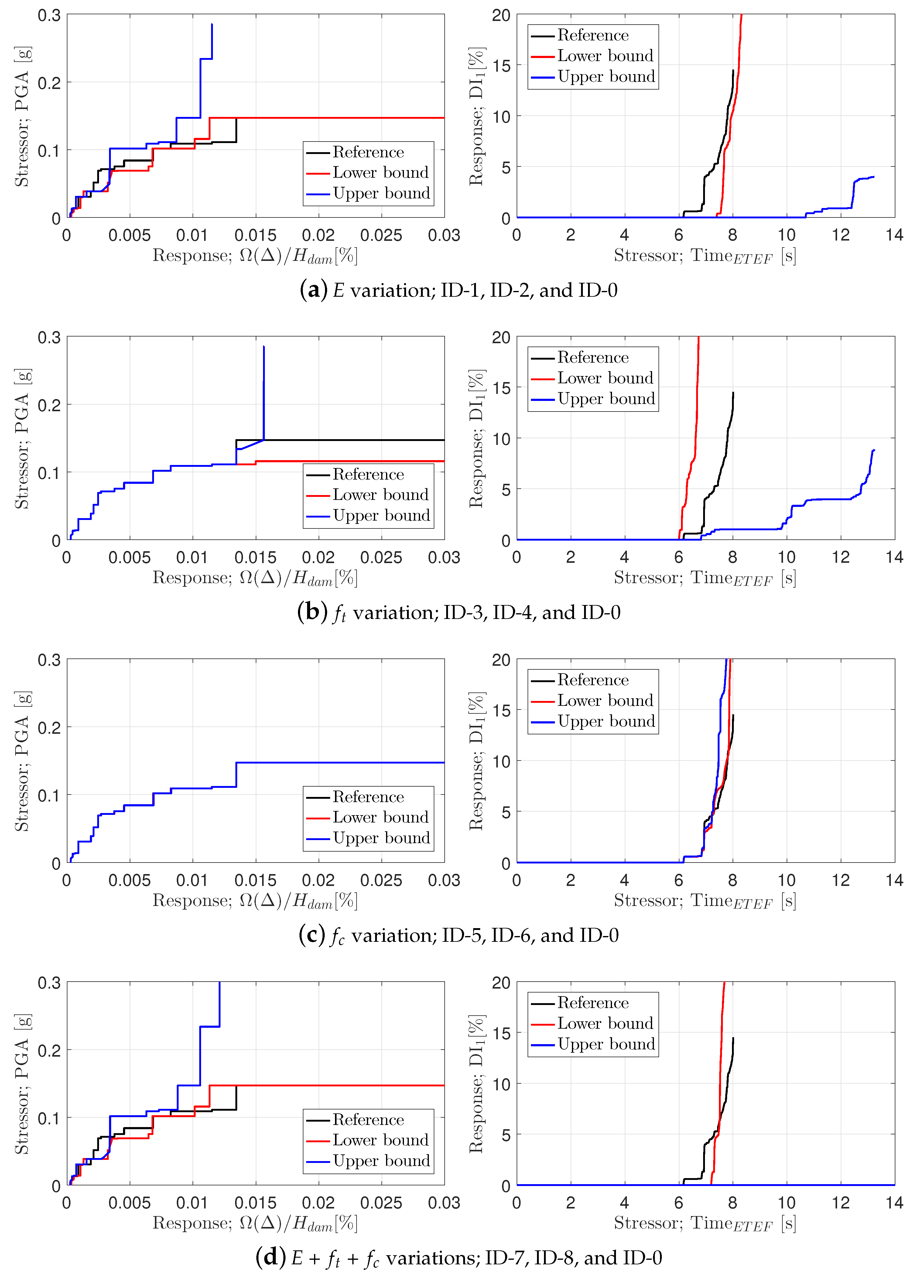
Three concrete parameters were assumed to be random variables (RVs), i.e., concrete modulus of elasticity, E, concrete tensile strength, , and compressive strength, . Nine different combinations are shown in Table 1. The first one, i.e., ID-0, was the reference simulation with all the properties at their mean value. Then, the properties took a lower bound (LB) and an upper bound (UB) one at a time (simulations ID-1–ID-6). Finally, two last simulations (i.e., ID-7 and ID-8) considered the combined effects of all three RVs.
Again, the buttress dam was modeled without any foundation and reservoir. The base of the dam was fixed, and an identical ETEF was applied in all cases. Subsequently, the crest displacement and the DI were recorded during the dynamic analysis. Results are summarized in Figure 7. For each of three RVs, and also the combined one, the displacement-based capacity functions are provided, which compare the UB and LB values with the reference one. Moreover, the evolution of DI is reported as a function of time. For the current purpose, only the first 13 s of the ETEF were applied, regardless of the damage level. The major observations can be summarized as follows:
- In a displacement-based capacity function (stressor-response coordinate system), the horizontal part corresponds to a large displacement with a small increase in the intensity level (i.e., numerical or physical) of failure. On the other hand, the vertical part shows the resistance of the dam (i.e., no or small drift with increasing seismic intensity).
- In general, lower and upper bound material properties decreased and increased the dynamic capacity, respectively. For example, in Figure 7b, the lower bound tensile strength, i.e., 2 MPa, reduced the dynamic capacity from 0.15 g to 0.11 g. On the other hand, the upper bound material property, i.e., 4 MPa, increased the dynamic capacity to about 0.3 g, where the analysis was not continued further.
- For the modulus of elasticity (see Figure 7a), the lower bound property reduced the dynamic capacity at pre-failure stages; however, it yielded to the same failure capacity of the reference analysis. One may note that the modulus of elasticity mainly controlled the initial stiffness of the system.
- According to Figure 7c, the compressive strength did not have any impact on the dynamic capacity of this dam. This can be attributed to the fact that the failure mode was covered by tensile damage (and not the compression damage).
- Finally, Figure 7d shows that the combined effect of all three RVs. The combined model was close to the one with only the modulus of elasticity as RV. The upper bound of the combined model did not show any damage (i.e., DI = 0) up to t = 15 s of analysis, where the simulation was terminated.
These plots clearly highlight the impact of uncertain parameters in developing the dynamic capacity functions for a dam. Although it is possible to perform some extra sensitivity analysis or even develop a response surface meta-model from these data [81], they are skipped in this paper.
4.3. Assessment of an Arch Dam Portfolio
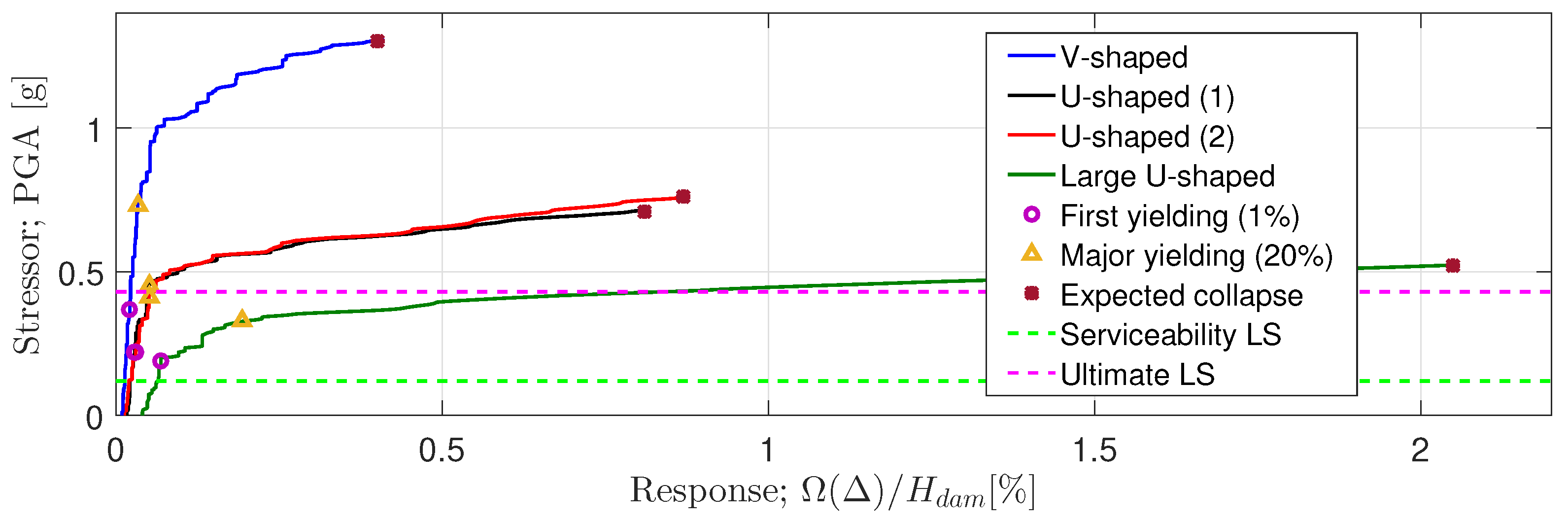
Arch and dome structures are characterized by having more key geometric parameters (i.e., curvatures). The shape of old dams has been defined during the design stage without considering explicitly the aspects related to the dynamic capacity of the structure. Figure 8 presents the relationship between the applied dynamic intensity and the response of the dams. According to the results obtained in this study, larger “U”-shaped dams appear to be the most vulnerable, while “V”-shaped dams provide higher seismic resistance. Each of the curves also shows key points associated with damages of the upstream and downstream faces of 1% and 20%, considered respectively minor and major yielding points. The relationship between these points and the associated serviceability and ultimate limit states, represented by dotted lines, gives an idea of the safety factor often translated in demand/capacity ratios. As mentioned previously, these ratios should be widely investigated and discussed to establish what can be defined as acceptable in terms of overall seismic safety.
According to the authors, it is not reasonable to associate the serviceability limit state with the attainment of the first crack. This is particularly true for numerical models with optimized meshes not able to capture localized damages. For this reason, it is recommended to set a value that can be associated with a measurable level of damages; the 20% value is proposed in this work. For the ultimate limit state, generally associated with the uncontrolled release of water, it is recommended to use the results obtained with the numerical model paying attention to the mechanism producing the limit state.
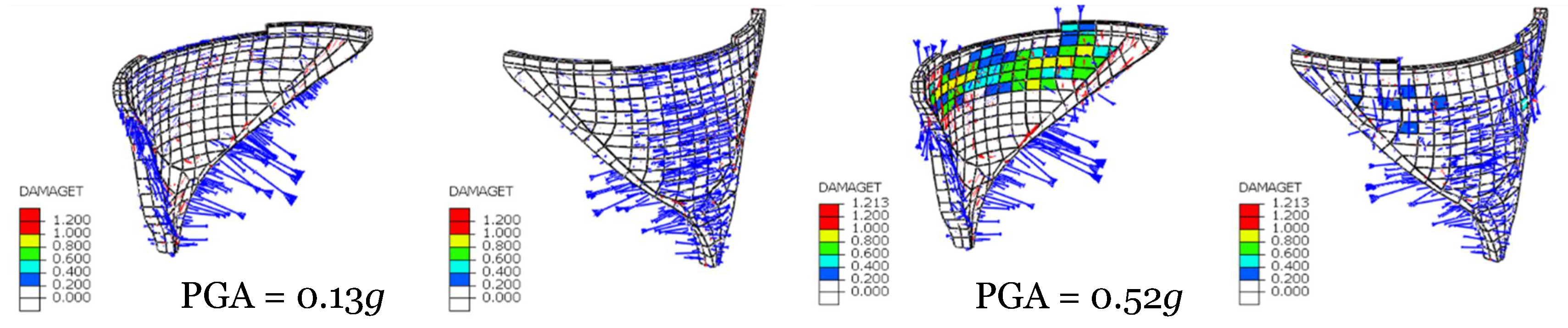
Figure 9 shows the “V”-shaped dam behavior for the serviceability (i.e., 0.13 g) and ultimate limit states (i.e., 0.52 g). For the low-intensity seismic action, the dam did not show any damage, and the compressive stresses (minimum principal stress: blue vectors) provided an effective arch behavior. As the applied dynamic load grew, the vertical joints started to open, and the cantilever effect appeared. The cantilever effect is one of the mechanisms able to produce horizontal cracks and redistribution of stresses. According to the simulations, “through cracks” started from the downstream face propagating towards the opposite face. In these cases, it is reasonable to think that one of the mechanisms able to produce the uncontrolled release of the water (or uncontrolled leakages) is the rocking of the isolated blocks at the top of the dam [82].
The attainment of the ultimate limit state in this condition should be defined using an appropriate model or independent procedures (i.e., hand calculation based on equilibrium). In the latter case, it will be necessary to establish the acceleration able to produce the overturning of the upper blocks in the upstream direction, information to be considered while the capacity curve for the dam is used. This is an example of special considerations required to use the capacity curves properly. If general rules or procedures cannot be defined because of the bespoke nature of arch dams, the proposed ETA method can be used as a tool to compare qualitatively the dynamic response of different structures or to have a better understanding of the impact of model assumptions over the seismic response. In this last context, the capacity function can be considered self-sufficient information.
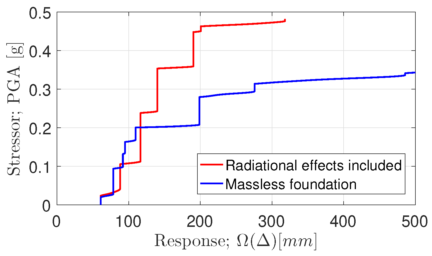
On the other hand, one of the most controversial issues in dynamic analysis of dams is the concept of “massed/massless foundation”. The massless foundation is a widely-adopted technique for practical seismic safety assessments of dams. Nevertheless, it has been extensively demonstrated that such a method provides over-conservative and misleading dam response [83]. To consider such effects properly, a drastic increase in the size and density of finite element domains is required [13]. Capacity functions, being able to represent the dam response in just one synthetic picture, can help to identify a critical PGA value beyond which the massless approach is no longer valid to achieve a consistent and realistic dam response; Figure 10. This critical PGA for Arch Dam #4 was about 0.2 g.
5. Present and Future Opportunities Offered by Capacity Functions
During the 3rd Meeting of EWG Dams and Earthquakes held in Lisbon [1], the authors presented the results of their studies and following a constructive collaboration with other researchers and professionals agreed on the expected goals for the incoming years. It appears that the research to be done on the seismic response of dams can be divided into two fields: the interpretation of recorded response and back-analysis under low to medium earthquakes and the forecast of the response of dams for strong earthquakes able to produce the uncontrolled release of the water or the collapse of the structure. Considering the different tools required for these two goals (i.e., nonlinear behavior capabilities versus extensive input parameter calibration), it is reasonable to think that the researchers working on these two fields will develop their own procedures and will feed different practices.
The most advanced (or latest) regulations and guidelines regarding the seismic assessment of existing dams are very demanding in terms of methods, resources, and time needed for its accomplishment. In some cases, the set of numerical simulations required may be economically unsustainable. Moreover, even if properly executed, the analyses are significantly affected by uncertainty, particularly when strong earthquakes have to be considered and strong nonlinear effects on construction joints and concrete are expected to occur. Uncertainties can be handled by calibrating the models with the real response of the dam, but from the experience collected so far, few dams’ experienced strong earthquakes able to activate substantially their nonlinear behavior [70]. It is worth mentioning that if something similar happened, the dam would likely be damaged enough to be dismissed or to be retrofitted significantly (i.e., new resisting concrete blocks), and this means the recorded data cannot be used. In this light, the information provided by the “capacity functions” can be very useful to make balanced decisions about the modeling and assessment assumptions addressed to the representation of the response for strong earthquakes. If this is the way forward, safety factors can be used to handle uncertainties. The shape of the capacity function or the key points can be post-processed to add some safety margins before decisions are made.
As mentioned previously, the capacity functions are also best positioned to facilitate the judgment of the safety factor available against failures for existing structures. This graphical form of the seismic response of the dams helps any decision-makers not having special expertise on the seismic response of dams to drive economic efforts for advanced studies or retrofitting works.
It is worth mentioning that standardized seismic functions such as those used in the ETA method may resolve major issues associated with the arbitrary selection of natural accelerograms. It is intuitive that it is hard to compare the seismic response of dams in the nonlinear field if the applied time histories are different. According to the experience of some of the authors, legislators are reluctant to use synthetic signals. This may represent a major obstacle for the ETA method and other similar methods. More recent studies on the generation of ETEF functions are addressing the main concerns received by the sector on their validity.
A proposal to receive the acceptance of these signals is to produce site-specific ETEF signals for different seismic regions able to represent more closely the soil and earthquake conditions. In this case, dams in the same region will be checked with the same signals defined by local codes. This appears to be a radical change from the design spectra approach, but is actually the most effective way to meet the new technical codes’ goals. This also might be a very good way to compare the seismic response of various dams and identify critical dams in a portfolio of dams.
Last but not least, for the most advantageous use of capacity functions, it is fundamental that the technical codes or the key institutions on dams’ safety define more appropriate acceptance limits for damages in both serviceability and collapse limit states.
6. Conclusions
Capacity functions are recognized in the building sector as a tool to judge the nonlinear behavior of framed structures. The advantages of their application seem remarkable and may be crucial within the seismic assessment procedures for concrete dams. A brief introduction to their use and the theoretical background was shown in this paper using some examples.
Following the recollection of some lessons learned on the seismic safety of dams located in high seismicity zones, the standard assessment procedures used by legislation and engineers were introduced. The new approach of “capacity functions” was then introduced for dams and the associated available methods briefly explained, in particular: incremental dynamic analysis (IDA), cloud analysis (CLA), and endurance time analysis (ETA). The last method was selected to show some advantages using capacity functions based on three examples: a concrete gravity dam, a buttress dam, and a portfolio of arch dams. The limits and the future enhancements of these seismic assessment procedures were also discussed.
Despite several applications of capacity functions in the dam industry, this procedure is still in a preliminary stage. The capacity functions may represent a powerful tool to meet some of the key requirements introduced by modern technical codes. The ETA method represents a good choice to determine the capacity functions with reasonable computational time.
The procedure introduced in the paper is focused mainly on the production of capacity curves. It is worth repeating that the modeling assumptions were not the subject of this work. Analysts doing the assessment must select the appropriate assumptions based on the best practice and the local legislation. If for the dam under assessment, it is crucial to consider special aspects such as galleries inside the dam, other structures connected to the dam (bridges, intake towers, or gates), reservoir sediments, foundation non-linearity, landslide effects, pore water pressure, dynamic uplift, lift joints, seismic input non-uniformity, or any other aspect, the analyst should select the appropriate modeling tools and adapt the procedure introduced here for the capacity function. In a certain sense, the main scope is to define a new way to add the shaking input and to get responses out of the numerical models prepared by the analysts, not a guide to set the numerical models.
It is the authors’ opinion that capacity functions in the form of standardized procedures will be available in the near future. Their comparison on a large scale will highlight crucial information of the seismic response of dams characterized by similar geometries and conditions.
Author Contributions
Conceptualization, L.F. and M.A.H.A.; methodology, L.F., M.M. and M.A.H.A.; software, L.F., M.A.H.A. and S.M.S.K.; validation, L.F., M.M. and M.A.H.A.; formal analysis, L.F. and S.M.S.K.; investigation, L.F. and M.A.H.A.; resources, L.F., M.M. and M.A.H.A; data curation, L.F. and M.A.H.A; writing—original draft preparation, L.F. and M.A.H.A.; writing—review and editing, L.F., M.M. and M.A.H.A.; supervision, M.A.H.A. and M.M.; project administration, M.A.H.A.
Funding
This research received no external funding.
Acknowledgments
The second author would like to express his sincere appreciation to Professor Victor E. Saouma (University of Colorado), and Dr. Jerzy W. Salamon (U.S. Bureau of Reclamation) for their support.
Conflicts of Interest
The authors declare no conflict of interest.
References
- Furgani, L.; Hariri-Ardebili, M.; Meghella, M. Towards the Seismic Capacity Assessment of Concrete Dams. In Proceedings of the 3rd Meeting of EWG Dams and Earthquakes, Lisbon, Portugal, 6–8 May 2019; pp. 87–98. [Google Scholar]
- USBR-Manual. Dam Safety Risk Analysis, Best Practices Training Manual; Version 2.2; Technical Report; U.S. Department of the Interior Bureau of Reclamation in Coorporation with the U.S. Army Corps of Engineers: Denver, CO, USA, 2011.
- Canadian Dam Association (CDA). Dam Safety Guidelines; Technical Report; Canadian Dam Association (CDA): Edmonton, AB, Canada, 2007. [Google Scholar]
- Decreto Ministeriale 26 Giugno 2014. E TRASPORTI, Ministero delle Infrastrutture. In Norme Tecniche per la Progettazione E la Costruzione degli Sbarramenti di Ritenuta (Dighe E Traverse). Gazzetta Ufficiale 07/07/2014 n.156; Technical Report; Gazzetta Ufficiale: Rome, Italy, 2004. [Google Scholar]
- NSW. Risk Management Policy Framework for Dam Safety; Technical Report; New South Wales Government Dams Safety Committee: Parramatta, NSW, Australia, 2006. [Google Scholar]
- Wieland, M. Features of seismic hazard in large dam projects and strong motion monitoring of large dams. Front. Arch. Civil Eng. China 2010, 4, 56–64. [Google Scholar] [CrossRef]
- Chopra, A.K. Earthquake analysis of arch dams: Factors to be considered. J. Struct. Eng. 2012, 138, 205–214. [Google Scholar] [CrossRef]
- Hariri-Ardebili, M.A.; Nuss, L.K. Seismic risk prioritization of a large portfolio of dams: Revisited. Adv. Mech. Eng. 2018, 10, 1687814018802531. [Google Scholar] [CrossRef]
- ICOLD. Selecting Seismic Parameters for Large Dams, Guidelines, Bulletin 148 (Revision of Bulletin 72); Technical Report; International Commission on Large Dams: Paris, France, 2010. [Google Scholar]
- Wieland, M. Seismic hazard and seismic design and safety aspects of large dam projects. In Perspectives on European Earthquake Engineering and Seismology; Springer: Berlin/Heidelberg, Germany, 2014; pp. 627–650. [Google Scholar]
- Fiorentino, G.; Furgani, L.; Magliano, S.; Nuti, C. Probabilistic evaluation of dam base sliding. In Proceedings of the 5th ECCOMAS Thematic Conference on Computational Methods in Structural Dynamics and Earthquake Engineering, Crete Island, Greece, 25–27 May 2015. [Google Scholar]
- Hariri-Ardebili, M.A.; Kianoush, M.R. Integrative seismic safety evaluation of a high concrete arch dam. Soil Dyn. Earthq. Eng. 2014, 67, 85–101. [Google Scholar] [CrossRef]
- Saouma, V.; Miura, F.; Lebon, G.; Yagome, Y. A simplified 3D model for soil-structure interaction with radiation damping and free field input. Bull. Earthq. Eng. 2011, 9, 1387–1402. [Google Scholar] [CrossRef]
- Bouaanani, N.; Lu, F. Assessment of potential-based fluid finite elements for seismic analysis of dam-reservoir systems. Comput. Struct. 2009, 87, 206–224. [Google Scholar] [CrossRef]
- Puntel, E.; Bolzon, G.; Saouma, V. Fracture Mechanics Based Model for Joints under Cyclic Loading. ASCE J. Eng. Mech. 2006, 132, 1151–1159. [Google Scholar] [CrossRef]
- Lee, J.; Fenves, G.L. A plastic-damage concrete model for earthquake analysis of dams. Earthq. Eng. Struct. Dyn. 1998, 27, 937–956. [Google Scholar] [CrossRef]
- Meghella, M.; Furgani, L. Application of Endurance Time Analysis Method to the NonLinear Seismic Analysis of dams: Potentialities and Limitations. In Proceedings of the 82nd Annual Meeting of ICOLD, Banff, AB, Canada, 4–5 October 2014. [Google Scholar]
- Hariri-Ardebili, M.A.; Mirzabozorg, H.; Estekanchi, H.E. Nonlinear seismic assessment of arch dams and investigation of joint behavior using endurance time analysis method. Arabian J. Sci. Eng. 2014, 39, 3599–3615. [Google Scholar] [CrossRef]
- Estekanchi, H.; Vafai, A.; Sadeghazar, M. Endurance time method for seismic analysis and design of structures. Sci. Iran. 2004, 11, 361–370. [Google Scholar]
- Darbre, G.R.; Schwager, M.; Panduri, R. Seismic safety evaluation of all large dams in Switzerland: Lessons learned. In Proceedings of the 26th International Congress on Large Dams, Vienna, Austria, 1–7 July 2018. [Google Scholar]
- OFEG. Sécurité des Ouvrages D’Accumulation—Documentation de Base Pour la Vérification des Ouvrages D’Accumulation aux Séismes; Technical Report; Officé Fedéral des Eaux et de la Géologie: Bern, Switzerland, 2003. [Google Scholar]
- Gosschalk, E.; Severn, R.; Charles, J.; Hinks, J. An Engineering Guide to Seismic Risk to Dams in the United Kingdom, and its international relevance. Soil Dyn. Earthq. Eng. 1994, 13, 163–179. [Google Scholar] [CrossRef]
- CFRB. Guidelines for the Justification of the Stability of Gravity Dams; Technical Report; Comité Francais des Barrages et Reservoirs: France, 2012. [Google Scholar]
- Royet, P.; Peyras, L. French guidelines for structural safety of gravity dams in a semi-probabilistic format. In Proceedings of the 9th ICOLD European Club Symposium (ITCOLD), Venice, Italy, 10–12 April 2013; p. 8. [Google Scholar]
- Mohan, K.J.; Kumar, R.P. Earthquakes and dams in India: An overview. Int. J. Civil Eng. Technol. 2013, 4, 6. [Google Scholar]
- Shimamoto, K. Trial implementation of new Japanese guidelines for seismic performance evaluation of dams during large earthquakes. In Proceedings of the 75th Annual Meeting of ICOLD, St. Petersburg, Russia, 24–27 June 2007. [Google Scholar]
- Tosun, H.; Zorluer, İ.; Orhan, A.; Seyrek, E.; Savaş, H.; Türköz, M. Seismic hazard and total risk analyses for large dams in Euphrates basin, Turkey. Eng. Geol. 2007, 89, 155–170. [Google Scholar] [CrossRef]
- Freeman, S. The capacity spectrum method. In Proceedings of the 11th European Conference on Earthquake Engineering, Paris, France, 6–11 September 1998. [Google Scholar]
- Fajfar, P. A nonlinear analysis method for performance based seismic design. Earthq. Spectra 2000, 16, 573–592. [Google Scholar] [CrossRef]
- Goel, R. Evaluation of modal and FEMA pushover procedures using strong-motion records of buildings. Earthq. Spectra 2005, 21, 653–684. [Google Scholar] [CrossRef]
- Ghanaat, Y. Failure modes approach to safety evaluation of dams. In Proceedings of the 13th World Conference on Earthquake Engineering, Vancouver, BC, Canada, 1–6 August 2004. [Google Scholar]
- Malm, R. Guideline for FE Analyses of Concrete Dams; Technical Report; Energiforsk: Stockholm, Sweden, 2016. [Google Scholar]
- Goldgruber, M.; Malm, R. Nonlinear Seismic Simulation of an Arch Dam using XFEM. In Proceedings of the Simulia Regional Users Meeting, Graz, Austria, 10 November 2014. [Google Scholar]
- ICOLD. Lessons from Dam Incidents, Complete Edition; Technical Report; International Commission on Large Dams: Paris, France, 1974. [Google Scholar]
- Boyer, D. Geologic factors influencing dam foundation failure modes. In Proceedings of the 26th Annual USSD Conference, San Antonio, TX, USA, 1–5 May 2006. [Google Scholar]
- Malm, R.; Hassanzadeh, M.; Hellgren, R. (Eds.) Numerical Analysis of Dams; ATCOLD, Austrian National Committee on Large Dams: Stockholm, Sweeden, 2018; pp. 1–722. [Google Scholar]
- Hariri-Ardebili, M.; Saouma, V. Single and multi-hazard capacity functions for concrete dams. Soil Dyn. Earthq. Eng. 2017, 101, 234–249. [Google Scholar] [CrossRef]
- Vamvatsikos, D.; Cornell, C. Applied incremental dynamic analysis. Earthq. Spectra 2004, 20, 523–553. [Google Scholar] [CrossRef]
- Vamvatsikos, D.; Cornell, C. Incremental dynamic analysis. Earthq. Eng. Struct. Dyn. 2002, 31, 491–514. [Google Scholar] [CrossRef]
- Sudret, B.; Der Kiureghian, A. Comparison of finite element reliability methods. Probab. Eng. Mech. 2002, 17, 337–348. [Google Scholar] [CrossRef]
- Zhang, Y.; Chen, G.; Zheng, L.; Li, Y.; Zhuang, X. Effects of geometries on three-dimensional slope stability. Can. Geotech. J. 2013, 50, 233–249. [Google Scholar] [CrossRef]
- Hariri-Ardebili, M.A.; Saouma, V.E. Quantitative failure metric for gravity dams. Earthq. Eng. Struct. Dyn. 2015, 44, 461–480. [Google Scholar] [CrossRef]
- Ansari, M.I.; Agarwal, P. Categorization of Damage Index of Concrete Gravity Dam for the Health Monitoring after Earthquake. J. Earthq. Eng. 2016, 20, 1222–1238. [Google Scholar] [CrossRef]
- Hariri-Ardebili, M.A.; Furgani, L.; Meghella, M.; Saouma, V.E. A new class of seismic damage and performance indices for arch dams via ETA method. Eng. Struct. 2016, 110, 145–160. [Google Scholar] [CrossRef]
- Vamvatsikos, D. Performing incremental dynamic analysis in parallel. Comput. Struct. 2011, 89, 170–180. [Google Scholar] [CrossRef]
- Alembagheri, M.; Ghaemian, M. Seismic assessment of concrete gravity dams using capacity estimation and damage indexes. Earthq. Eng. Struct. Dyn. 2013, 42, 123–144. [Google Scholar] [CrossRef]
- Pan, J.; Xu, Y.; Jin, F. Seismic performance assessment of arch dams using incremental nonlinear dynamic analysis. Eur. J. Environ. Civ. Eng. 2015, 19, 305–326. [Google Scholar] [CrossRef]
- Alembagheri, M.; Seyedkazemi, M. Seismic performance sensitivity and uncertainty analysis of gravity dams. Earthq. Eng. Struct. Dyn. 2015, 44, 41–58. [Google Scholar] [CrossRef]
- Alembagheri, M.; Ghaemian, M. Incremental dynamic analysis of concrete gravity dams including base and lift joints. Earthq. Eng. Eng. Vib. 2013, 12, 119–134. [Google Scholar] [CrossRef]
- Chen, D.H.; Yang, Z.H.; Wang, M.; Xie, J.H. Seismic performance and failure modes of the Jin’anqiao concrete gravity dam based on incremental dynamic analysis. Eng. Fail. Anal. 2019, 100, 227–244. [Google Scholar] [CrossRef]
- Soysal, B.; Binici, B.; Arici, Y. Investigation of the relationship of seismic intensity measures and the accumulation of damage on concrete gravity dams using incremental dynamic analysis. Earthq. Eng. Struct. Dyn. 2016, 45, 719–737. [Google Scholar] [CrossRef]
- Hariri-Ardebili, M.; Saouma, V. Collapse Fragility Curves for Concrete Dams: Comprehensive Study. ASCE J. Struct. Eng. 2016, 142, 04016075. [Google Scholar] [CrossRef]
- Rezaeian, S.; Der Kiureghian, A. Simulation of synthetic ground motions for specified earthquake and site characteristics. Earthq. Eng. Struct. Dyn. 2010, 39, 1155–1180. [Google Scholar] [CrossRef]
- Shome, N. Probabilistic Seismic Demand Analysis of Nonlinear Structures. Ph.D. Thesis, Stanford University, Stanford, CA, USA, 1999. [Google Scholar]
- Estekanchi, H.; Valamanesh, V.; Vafai, A. Application of endurance time method in linear seismic analysis. Eng. Struct. 2007, 29, 2551–2562. [Google Scholar] [CrossRef]
- Valamanesh, V.; Estekanchi, H.; Vafai, A.; Ghaemian, M. Application of the endurance time method in seismic analysis of concrete gravity dams. Sci. Iran. 2011, 18, 326–337. [Google Scholar] [CrossRef] [Green Version]
- Hariri-Ardebili, M.A.; Saouma, V.; Porter, K.A. Quantification of seismic potential failure modes in concrete dams. Earthq. Eng. Struct. Dyn. 2016, 45, 979–997. [Google Scholar] [CrossRef]
- Nozari, A.; Estekanchi, H. Optimization of endurance time acceleration functions for seismic assessment of structures. Int. J. Optim. Civ. Eng. 2011, 1, 257–277. [Google Scholar]
- Mashayekhi, M.; Estekanchi, H. Investigation of Non-Linear Cycles’ Properties in Structures Subjected to Endurance Time Excitation Functions. Int. J. Optim. Civ. Eng. 2013, 3, 239–257. [Google Scholar]
- Mashayekhi, M.; Estekanchi, H.E.; Vafai, H.; Mirfarhadi, S.A. Development of hysteretic energy compatible endurance time excitations and its application. Eng. Struct. 2018, 177, 753–769. [Google Scholar] [CrossRef]
- Mashayekhi, M.; Estekanchi, H.; Vafai, H. Simulation of Endurance Time Excitations Using Increasing Sine Functions. Int. J. Optim. Civ. Eng. 2019, 9, 65–77. [Google Scholar]
- Mashayekhi, M.; Estekanchi, H.E.; Vafai, H.; Ahmadi, G. An evolutionary optimization-based approach for simulation of endurance time load functions. Eng. Optim. 2019, 1–20. [Google Scholar] [CrossRef]
- Krawinkler, H. Report No. ATC 24: Guidelines for Cyclic Seismic Testing of Components of Steel Structures; Technical Report; Applied Technology Council: Redwood City, CA, USA, 1992. [Google Scholar]
- Filiatrault, A.; Wanitkorkul, A.; Constantinou, M. Development and Appraisal of a Numerical Cyclic Loading Protocol for Quantifying Building System Performance; Technical Report MCEER-08-0013; University at Buffalo, State University of New York: New York, NY, USA, 2008. [Google Scholar]
- Hariri-Ardebili, M.A.; Mirzabozorg, H. Estimation of probable damages in arch dams subjected to strong ground motions using endurance time acceleration functions. KSCE J. Civ. Eng. 2014, 18, 574–586. [Google Scholar] [CrossRef]
- ICOLD. Design Features of Dams to Effectively Resist Seismic Ground Motion, Bulletin 120; Technical Report; International Commission on Large Dams: Paris, France, 2001. [Google Scholar]
- USCOLD. Observed Performance of Dams during Earthquakes; Technical Report; U.S. Committee on Large Dams: Denver, CO, USA, 1992. [Google Scholar]
- USCOLD. Observed Performance of Dams during Earthquakes; Technical Report; U.S. Committee on Large Dams: Denver, CO, USA, 2000; Volume 2. [Google Scholar]
- USSD. Observed Performance of Dams during Earthquakes; Technical Report; U.S. Society on Dams: Denver, CO, USA, 2014; Volume 3. [Google Scholar]
- Nuss, L.; Matsumoto, N.; Hansen, K. Shaken, But Not Stirred—Earthquake Performance of Concrete Dams. In Proceedings of the 32nd USSD Annual Meeting and Conference: Innovative Dam and Levee Design and Construction for Sustainable Water Management, New Orleans, LA, USA, 23–27 April 2012. [Google Scholar]
- Chowdhury, M.; Matheu, E.; Hall, R. Shake table experiment of a 1/20-Scale Koyna dam model. In Proceedings of the 19th International Modal Analysis Conference, IMAC XIX, Hyatt Orlando, Kissimmee, FL, USA, 5–8 February 2001. [Google Scholar]
- Wilcoski, J.; Robert, R.; Matheu, E.; Gambill, J.; Chowdhury, M. Seismic Testing of a 1/20 Scale Model of Koyna Dam; Report No. ERDC TR-01-17; Technical Report; U.S. Army Corps of Engineers, Engineering Research and Development Center: Washington, DC, USA, 2001. [Google Scholar]
- Salamon, J.; Nuss, L. Design of Double-Curvature Arch Dams Planning, Appraisal, Feasibility Level; Technical Report; U.S. Department of the Interior Bureau of Reclamation: Denver, CO, USA, 2012.
- Ghaemian, M. Seismic Response of a Retrofitted Concrete Buttress Dam. In Proceedings of the 11th World Conference on Earthquake Engineering, Acapulco, Mexico, 23–28 June 1996. [Google Scholar]
- Hariri-Ardebili, M.A.; Seyed-Kolbadi, S.M. Seismic cracking and instability of concrete dams: Smeared crack approach. Eng. Fail. Anal. 2015, 52, 45–60. [Google Scholar] [CrossRef]
- Hariri-Ardebili, M.A.; Kianoush, M.R. Seismic analysis of a coupled dam-reservoir foundation system considering pressure effects at opened joints. Struct. Infrastruct. Eng. 2015, 11, 833–850. [Google Scholar] [CrossRef]
- EN-1998. Eurocode-8: Design of Structures for Earthquake Resistance; Technical Report; The European Union Per Regulation: Brussels, Belgium, 2004. [Google Scholar]
- Saouma, V. Numerical Modeling of AAR; CRC Press: Boca Raton, FL, USA, 2014. [Google Scholar]
- Hariri-Ardebili, M.A.; Seyed-Kolbadi, S.M.; Noori, M. Response Surface Method for Material Uncertainty Quantification of Infrastructures. Shock Vib. 2018, 2018, 1784203. [Google Scholar] [CrossRef]
- Hariri-Ardebili, M.A.; Saouma, V.E. Sensitivity and Uncertainty Quantification of the Cohesive Crack Model. Eng. Fract. Mech. 2016, 155, 18–35. [Google Scholar] [CrossRef]
- Hariri-Ardebili, M.A. MCS-based response surface metamodels and optimal design of experiments for gravity dams. Struct. Infrastruct. Eng. 2018, 14, 1641–1663. [Google Scholar] [CrossRef]
- Malla, S.; Wieland, M. Analysis of an arch gravity dam with a horizontal crack. Comput. Struct. 1999, 72, 267–278. [Google Scholar] [CrossRef]
- Hariri-Ardebili, M.A.; Saouma, V.E. Impact of Near-fault vs. Far-field Ground Motions on the Seismic Response of an Arch Dam with Respect to Foundation Type. Dam Eng. 2014, 24, 19–52. [Google Scholar]
Figure 1.
Sample incremental dynamic analysis (IDA) capacity functions for concrete dams: (a) gravity dam [46], (b) arch dam [47], (c) gravity dam [48], (d) gravity dam [49], (e) gravity dam [43], (f) arch dam [50], (g) gravity dam [51], and (h) gravity dam [52]. PGA, peak ground acceleration.

Figure 2.
Sample cloud analysis (CLA) capacity functions for concrete dams. (a) Linear analysis; (b) nonlinear analysis. IM, intensity measurement; S, scenario.
Figure 2.
Sample cloud analysis (CLA) capacity functions for concrete dams. (a) Linear analysis; (b) nonlinear analysis. IM, intensity measurement; S, scenario.

Figure 3.
Sample endurance time excitation function (ETEF). (a) Acceleration time history; (b) time-dependent response spectra.
Figure 3.
Sample endurance time excitation function (ETEF). (a) Acceleration time history; (b) time-dependent response spectra.

Figure 4.
Comparing the cyclic pushover and dynamic pushover methods to develop capacity functions; is displacement, F force, and a acceleration.
Figure 4.
Comparing the cyclic pushover and dynamic pushover methods to develop capacity functions; is displacement, F force, and a acceleration.

Figure 5.
Finite element models for the dam body. Note: the foundation and reservoir are not shown for gravity and arch dams.
Figure 5.
Finite element models for the dam body. Note: the foundation and reservoir are not shown for gravity and arch dams.

Figure 6.
Computed capacity functions for the case study gravity dam; PGA is peak ground acceleration; Cr refers to cracking; DI is the damage index; is displacement. (a) Displacement-based curve; (b) DI-based curves; (c) damage profiles at two different times.
Figure 6.
Computed capacity functions for the case study gravity dam; PGA is peak ground acceleration; Cr refers to cracking; DI is the damage index; is displacement. (a) Displacement-based curve; (b) DI-based curves; (c) damage profiles at two different times.

Figure 7.
Computed capacity functions for the case study buttress dam; PGA is peak ground acceleration; DI is the damage index; is displacement. (a) E variation; ID-1, ID-2, and ID-0; (b) variation; ID-3, ID-4, and ID-0; (c) variation; ID-5, ID-6, and ID-0; (d) E + + variations; ID-7, ID-8, and ID-0.

Figure 8.
Computed displacement-based capacity functions for an arch dam portfolio; PGA is peak ground acceleration; is displacement; LS refers to the limit state.
Figure 8.
Computed displacement-based capacity functions for an arch dam portfolio; PGA is peak ground acceleration; is displacement; LS refers to the limit state.

Figure 9.
Damage state for dams at two different seismic intensities; PGA = 0.13 g (serviceability limit state); and PGA = 0.52 g (ultimate limit state).
Figure 9.
Damage state for dams at two different seismic intensities; PGA = 0.13 g (serviceability limit state); and PGA = 0.52 g (ultimate limit state).

Figure 10.
Capacity functions for Arch Dam #4 with two foundation models; PGA is peak ground acceleration; is displacement.
Figure 10.
Capacity functions for Arch Dam #4 with two foundation models; PGA is peak ground acceleration; is displacement.


Table 1.
Material combination for the case study buttress dam. LB, lower bound; UB, upper bound.
| Simulation | E (GPa) | (MPa) | (MPa) | (kg/m) | (-) |
|---|---|---|---|---|---|
| ID-0 (Ref) | 35 | 35 | 3 | 2400 | 0.15 |
| ID-1 (LB) | 30 | 35 | 3 | 2400 | 0.15 |
| ID-2 (UB) | 40 | 35 | 3 | 2400 | 0.15 |
| ID-3 (LB) | 35 | 35 | 2 | 2400 | 0.15 |
| ID-4 (UB) | 35 | 35 | 4 | 2400 | 0.15 |
| ID-5 (LB) | 35 | 30 | 3 | 2400 | 0.15 |
| ID-6 (UB) | 35 | 40 | 3 | 2400 | 0.15 |
| ID-7 (LB) | 30 | 30 | 2 | 2400 | 0.15 |
| ID-8 (UB) | 40 | 40 | 4 | 2400 | 0.15 |
© 2019 by the authors. Licensee MDPI, Basel, Switzerland. This article is an open access article distributed under the terms and conditions of the Creative Commons Attribution (CC BY) license (http://creativecommons.org/licenses/by/4.0/).
Share and Cite
MDPI and ACS Style
Furgani, L.; Hariri-Ardebili, M.A.; Meghella, M.; Seyed-Kolbadi, S.M. On the Dynamic Capacity of Concrete Dams. Infrastructures 2019, 4, 57. https://doi.org/10.3390/infrastructures4030057
AMA Style
Furgani L, Hariri-Ardebili MA, Meghella M, Seyed-Kolbadi SM. On the Dynamic Capacity of Concrete Dams. Infrastructures. 2019; 4(3):57. https://doi.org/10.3390/infrastructures4030057
Chicago/Turabian StyleFurgani, L., M. A. Hariri-Ardebili, M. Meghella, and S. M. Seyed-Kolbadi. 2019. "On the Dynamic Capacity of Concrete Dams" Infrastructures 4, no. 3: 57. https://doi.org/10.3390/infrastructures4030057