Article

A Novel Multi-Attribute Decision Making Method Based on The Double Hierarchy Hesitant Fuzzy Linguistic Generalized Power Aggregation Operator

School of Management Science and Engineering, Shandong University of Finance and Economics, Jinan 250014, China
*
Author to whom correspondence should be addressed.
Information 2019, 10(11), 339; https://doi.org/10.3390/info10110339
Submission received: 14 October 2019 / Revised: 28 October 2019 / Accepted: 28 October 2019 / Published: 30 October 2019
(This article belongs to the Section Information Theory and Methodology)

Abstract

:
A double hierarchy hesitant fuzzy linguistic term set (DHHFLT) is deemed as an effective and powerful linguistic expression which models complex linguistic decision information more accurately by using two different hierarchy linguistic term sets. The purpose of this paper is to propose a multi-attribute decision making method to tackle complex decision issues in which attribute values are represented as double hierarchy hesitant fuzzy linguistic numbers, and there are some extreme or unreasonable data in the attribute values. To do this, firstly, four double hierarchy hesitant fuzzy linguistic generalized power aggregation operators are introduced, including the double hierarchy hesitant fuzzy linguistic generalized power average (DHHFLGPA) operator, the double hierarchy hesitant fuzzy linguistic generalized power geometric (DHHFLGPG) operator, and their weighted forms. Thereafter, several favorable properties, as well as representative cases of the proposed operators, are investigated in detail. Moreover, by virtue of the proposed operators, a novel approach is developed for coping with multi-attribute decision making cases in the double hierarchy hesitant fuzzy linguistic context. Finally, an illustrated example is given to demonstrate the practical application of the presented approach, an availability verification is given to show its validity, and a comparative analysis is also conducted to highlight the advantages of the proposed approach.

1. Introduction

Multiple attribute decision making (MADM) occupies a significant position in modern decision science. It aims to find out the most satisfying alternative from the given alternatives in accordance with the assessments given by decision-makers (DMs) among different attributes [1,2,3,4,5]. In practical evaluating issues, with the rising complexity of the social environment and the subjectivity and ambiguity inherent in human thought, attribute values under different alternatives are uncertain or vague for the most part [6,7,8]. Therefore, it might be more accurate to depict DM’s evaluation information in qualitative form than quantitative form. For instance, when assessing a car’s design, qualitative descriptions like “good” and “perfect” rather than crisp numbers are used [9]. Thus, Zadeh [10] first proposed the concept of fuzzy linguistic variable, and since then various linguistic representation forms arose for the past few years, such as the linguistic models on account of type-2 fuzzy sets [11], 2-tuple linguistic mode [12], hesitant fuzzy linguistic term set (HFLTS) [13], probability linguistic term set [14], etc. Among these models, the concept of HFLTS was originally defined by Rodríguez et al. [13] by combining the hesitant fuzzy sets [15] and linguistic variable, which allows DMs to hesitate in several possible linguistic terms. Therefore, the application of HFLTS is more aligned with the cognitive and expression habits of DMs. The HFLTS has gained great success as it can be used to represent several linguistic terms or comparative linguistic expressions together with some context-free grammars [16,17]. Now and in the future, decision-making methodologies and algorithms with hesitant fuzzy linguistic models are a quite promising research line representing a high-quality breakthrough in this topic. Over recent years, HFLTS has been deeply probed by quite a few scholars from different perspectives [18,19,20,21].
However, as Gou et al. mentioned in Ref. [14], in some complex decision-scenarios, HFLTSs may fail to express fully and comprehensively the redefined evaluation preferences of DMs. As an example, let S = { ς 1 , ς 2 , ς 3 , ς 4 , ς 5 , ς 6 , ς 7 } = { w o r s t , v e r y p o o r , p o o r , m e d i u m , f i n e , v e r y f i n e , p e r f e c t } be a linguistic term set (LTS), then we can utilize { ς 3 , ς 2 } , { ς 2 , ς 1 , ς 0 } and { ς 3 } to describe the linguistic expressions “worse than very poor”, “between very poor and medium” and “perfect”, respectively. Nevertheless, in many cases, we might resort to some more meticulous linguistic terms (LTs) to comprehensively depict our views just as “only a bit high”, “exactly right medium”, “much fine”, etc. Considering that there are no linguistic models suitable for expressing such intricate linguistic information, Gou et al. [14] have given the definition of double hierarchy linguistic term sets (DHLTS), which are made up of two hierarchy LTSs in which the internal hierarchy LTS is used to make a further description or elaborate explanation for every LT contained in the external hierarchy LTS. Thereafter, they presented the double hierarchy hesitant fuzzy linguistic (DHHFL) term sets (DHHFLTS) [14] via extending DHLTS to the hesitant fuzzy circumstance. DHHFLTS is pretty available in managing situations where DMs hesitate between several complex LTs when presenting their views on alternatives in the course of decision-making, and it has become a project of widespread concern to researchers. Lately, Gou et al. further presented a number of distance and similarity measures of DHHFL elements (DHHFLEs) [22] and developed a process of reaching a common agreement in large-scale group decision making (GDM) using DHHFL preference relationship [23]. Liu et al. [24] investigated a DHHFL mathematical programming means for multi-attribute GDM problems. Krishankumar et al. [25] have given a novel decision framework in the context of DHHFLTS, etc.
For the past few years, the methods to aggregate the assessment information provided by DMs have also aroused abundant researchers’ concerns in the area of decision science [26,27,28]. The aggregation operators occupy a vitally important situation in the progress of information infusion. The prominent strength of using aggregation operators to aggregate the evaluation information is that it can fully consider the evaluation data and obtain the ranking of alternatives expressly. Up to now, many scholars have systematically studied the information aggregation operators from various aspects. Harsanyi [29] introduced the weighted averaging (WA) operator. On that basis, Yager [30] presented an ordered weighted aggregation (OWA) operator. Then with the deepening and development of research, some considerable operators are proposed, such as Heronian mean (HM) [31] operator and Bonferroni mean (BM) [32] operator. Nonetheless, a majority of the existing aggregation operators fail to take the generality and extremity of the values giving by DMs into consideration. Therefore, Yager [33] put forward to the power average (PA) operator that took the support degree between any two inputs into consideration. The most attractive advantage of the PA is that it can weaken the unreasonable extreme evaluation values on results ranking. Furthermore, Zhou [34] defined the generalized PA (GPA) operator, which is the development of the PA operator in a generalized form. Since then, vast extensions of the GPA operator have been excavated for different situations. Liu et al. presented the intuitionistic linguistic power generalized WA (ILPGWA) operator [35] through extending the GPA operator to the intuitionistic linguistic set, 2-dimension uncertain linguistic GPA (2DULGPA) operator [36] as well as intuitionistic trapezoidal fuzzy power generalized weighted average operator [37]. Wu et al. [38] introduced 2-tuple linguistic GPA operator and interval 2-tuple linguistic GPA operator, etc.
Despite the fact that DHHFLTS is pretty useful in handling situations where DMs hesitate between several complex LTs when presenting their views in the progress of decision-making, the extant approaches with respect to the DHHFLTS cannot take the support degree between any two inputs into consideration and fails to handle the presence of extreme values. At the same time, the extensions of the GPA operator cannot deal with the assessment values expressed in DHHFLTS form. Therefore, motivated by the GPA operator, the focus of this paper is to stretch the GPA operator to the DHHFLT circumstance and present the DHHFLGPA operator and DHHFL generalized power geometric (DHHFLGPA) operator, which can make a combination of the strengths of the DHHFLTS and GPA operator. Then we apply them to solve MADM problems and present a novel MADM method.
The following part of this paper can be arranged as follows: Section 2 gives a general retrospect of some corresponding concepts, such as the DHHFLTS, its operational laws and GPA operator. Section 3 proposes some generalized power operators with respect to DHHFLES, then several properties as well as particular cases are provided. In Section 4, we put forward a novel MADM approach on account of presented operators. Section 5 presents with an instance to manifest the superiority of the presented approach. This paper comes to a conclusion in Section 6.

2. Preliminaries

2.1. Double Hierarchy Hesitant Fuzzy Linguistic Term Set

Definition 1.
[14] Given the first hierarchy LTS (FHLTS) S = { ς t | t = ε , , 1 , 0 , 1 , , ε } and the second hierarchy LTS (SHLTS) θ = { ϑ κ | κ = ι , , 1 , 0 , 1 , , ι } , and these two layers are entirely independent of each other. Then the mathematical form of DHLTS S θ can be expressed as,
S θ = { ς t < ϑ κ > | t = ε , , 1 , 0 , 1 , , ε ; κ = ι , , 1 , 0 , 1 , , ι } .
ς t < ϑ κ > is referred to double hierarchy linguistic term (DHLT), in which ϑ κ indicates its corresponding second hierarchy LT as ς t is the first hierarchy LT. Furthermore, the SHLTS may be different under the different first hierarchy LT.
For example, let t = ε = 3 , the allocations of four different forms of the SHLTS are shown in Figure 1 [14].
Remark 1.
In Figure 1, when ε takes the different values, there are four different situations of the corresponding second hierarchy LTS, if ε 0 , which means that the valence of the first hierarchy LTS is active, thus the level of the element contained in the second hierarchy LTS should be arranged from low to high. By contrast, the level of the first hierarchy LTS is passive when ε 0 , thus the valence of the element contained in the second hierarchy LTS should be given from high to low. In particular, since both ς ε and ς ε merely contain a one-sided domain, we simply apply θ = { ϑ κ | κ = ι , , 1 , 0 } and θ = { ϑ κ | κ = 0 , 1 , , ι } to depict ς ε and ς ε , respectively.
Moreover, Gou et al. [14] applied S θ to hesitant fuzzy environment and introduced the DHHFL term set as shown below,
Definition 2.
Let S θ = { ς t < ϑ κ > | t = ε , 1 , 0 , 1 , , ε ; κ = ι , , 1 , 0 , 1 , , ι } be a DHLTS. Then the mathematical form of DHHFL term set (DHHFLTS) on X can be shown as,
H S θ = { < x i , h S θ ( x i ) > | x i X }
In which h S θ ( x i ) is a collection of several elements in S θ , indicating all of the concern membership degrees of x i to H S θ , denoted as
h S θ ( x i ) = { ς t r < ϑ κ r > ( x i ) | ς t r < ϑ κ r > S θ ; t = ε , , 1 , 0 , 1 , , ε ; κ = ι , , 1 , 0 , 1 , , ι ; r = 1 , 2 , , # L } ,
with #L indicating the amount of DHLTs in h S θ ( x i ) , ς t r < ϑ κ r > ( x i ) ( r = 1 , 2 , , # L ) in certain h S θ ( x i ) representing the elements in S θ . For the sake of simplicity, we call h S θ ( x i ) the DHHFL element (DHHFLE), and the set of all DHHFLEs is Φ Ψ .
Next, according to the discussion of monotonic function, Gou et al. [14] proposed two monotonic functions for making the interconversion between DHLTs and real numbers and extended it into a continuous representation.
Definition 3.
Let S θ = { ς t < ϑ κ > | t = ε , , 1 , 0 , 1 , , ε ; κ = ι , , 1 , 0 , 1 , , ι } be a DHLTS, h S θ = { ς t r < ϑ κ r > | ς t r < ϑ κ r > S θ ; t = ε , , 1 , 0 , 1 , , ε ; κ = ι , , 1 , 0 , 1 , , ι ; r = 1 , 2 , , # L } , h α = { α r | 0 α r 1 ; r = 1 , 2 , , # L } be a DHHFLE and a hesitant fuzzy element (HFE), respectively, where #L is the amount of LTs in h S θ . Then the suffix ς t r < ϑ κ r > of the DHLT ς t r < ϑ κ r > and the membership degree α r that conveys the identical significance with the DHLT ς t r < ϑ κ r > can make mutual conversion to each other by the following functions γ and γ 1
γ : [ ε , ε ] × [ ι , ι ] [ 0 , 1 ] , γ ( t r , κ r ) = { 1 ε × κ r + ι 2 ι + ε + t r 1 2 ε = κ l + ( t r + ε ) ι 2 ε ι = α l , i f ε + 1 t r ε 1. 1 2 ε × κ r + ι ι + ε + t r 1 2 ε = κ r + ( t r + ε ) ι 2 ε ι = α r , i f t r = ε . 1 2 ε × κ r ι = κ r 2 ε ι = α r , i f t r = ε .
γ 1 : [ 0 , 1 ] [ ε , ε ] × [ ι , ι ] , γ 1 ( α r ) = { S < ϑ ι ( ) > , i f 1 < ε ; S 0 < ϑ ι ( ) > , i f 1 < 1 ; S 1 + < ϑ ι ( 1 ) > , i f ε < 1.
In which = 2 ε α r ε . In that way, the conversion functions H and H 1 between the DHHFLE h S θ and the HFE h α are given as follows, respectively,
H : Φ Ψ Ξ , H ( h S θ = { ς t r < ϑ κ r > | ς t r < ϑ κ r > S θ ; t = [ ε , ε ] ; κ = [ ι , ι ] ; r = 1 , 2 , , # L } ) = { α r | α r = γ ( t r , κ r ) } = h α
H 1 : Ξ Φ Ψ , H 1 ( h α ) = H 1 ( { α r | α r [ 0 , 1 ] ; r = 1 , 2 , , # L } ) = { ς t r < ϑ κ r > | t r < ϑ κ r > = γ 1 ( α r ) } = h S θ .
Definition 4.
Let S θ = { ς t < ϑ κ > | t = ε , , 1 , 0 , 1 , , ε ; κ = ι , , 1 , 0 , 1 , , ι } be a DHLTS, h S θ = { ς t r < ϑ κ r > | ς t r < ϑ κ r > S θ ; t = [ ε , ε ] ; κ = [ ι , ι ] ; r = 1 , 2 , , # L } , h S θ 1 = { ς 1 t r < ϑ κ r > | ς 1 t r < ϑ κ r > S θ ; κ = [ ι , ι ] ; r = 1 , 2 , , # L } , h S θ 2 = { ς 2 t r < ϑ κ r > | ς 2 t r < ϑ κ r > S θ ; t = [ ε , ε ] ; κ = [ ι , ι ] ; r = 1 , 2 , , # L } be three DHHFLEs, λ be a nonnegative number. Then
(1) h S θ 1 h S θ 2 = H 1 ( ρ 1 H ( h S θ 1 ) , ρ 2 H ( h S θ 2 ) { ρ 1 + ρ 2 ρ 1 ρ 2 } ) ,
(2) h S θ 1 h S θ 2 = H 1 ( ρ 1 H ( h S θ 1 ) , ρ 2 H ( h S θ 2 ) { ρ 1 ρ 2 } ) ,
(3) λ h S θ = H 1 ( ρ H ( h S θ ) { 1 ( 1 ρ ) λ } ) ,
(4) h S θ λ = H 1 ( ρ H ( h S θ ) { ρ λ } ) ,
(5) ( h S θ ) c = H 1 ( ρ H ( h S θ ) { 1 ρ } ) .
Example 1.
Given a DHLTS S θ = { ς t < ϑ κ > | t = 3 , , 1 , 0 , 1 , , 3 ; κ = 3 , , 1 , 0 , 1 , , 3 } . Assume there are two DHHFLEs h S θ 1 = { ς 1 < ϑ 2 > , ς 2 < ϑ 1 > } and h S θ 2 = { ς 0 < ϑ 1 > , ς 0 < ϑ 3 > , ς 1 < ϑ 2 > } , as well as a real number λ = 1 / 3 , we have,
(1) h S θ 1 h S θ 2 = H 1 ( ρ 1 H ( h S θ 1 ) , ρ 2 H ( h S θ 2 ) { ρ 1 + ρ 2 ρ 1 ρ 2 } ) = H 1 { 4 9 + 5 9 4 9 × 5 9 , 4 9 + 2 3 4 9 × 2 3 , 4 9 + 7 9 4 9 × 7 9 , 8 9 + 5 9 8 9 × 5 9 , 8 9 + 2 3 8 9 × 2 3 , 8 9 + 7 9 8 9 × 7 9 } = { ς 1 < ϑ 1.53 , ϑ 2.67 > , ς 2 < ϑ 0.975 , ϑ 2.1 , ϑ 2.34 , ϑ 2.55 > } ;
(2) h S θ 1 h S θ 2 = H 1 ( ρ 1 H ( h S θ 1 ) , ρ 2 H ( h S θ 2 ) { ρ 1 ρ 2 } ) = H 1 { 4 9 × 5 9 , 4 9 × 2 3 , 4 9 × 7 9 , 8 9 × 5 9 , 8 9 × 2 3 , 8 9 × 7 9 } = { ς 1 < ϑ 1.56 , ϑ 0.66 > , ς 0 < ϑ 2.79 , ϑ 0.12 , ϑ 1.68 > , ς 1 < ϑ 0.45 > } ;
(3) λ h S θ 1 = H 1 ( ρ H ( h S θ 1 ) { 1 ( 1 ρ ) λ } ) = H 1 { 1 ( 1 4 9 ) 1 / 3 , 1 ( 1 8 9 ) 1 / 3 } = { ς 1 < ϑ 2.976 > , ς 0 < ϑ 0.36 > } ;
(4) h S θ 1 λ = H 1 ( ρ H ( h S θ ) { ρ λ } ) = H 1 { ( 4 9 ) 1 / 3 , ( 8 9 ) 1 / 3 } = { ς 1 < ϑ 1.73 > , ς 2 < ϑ 2.31 > } ;
(5) ( h S θ 1 ) c = H 1 ( ρ H ( h S θ ) { 1 ρ } ) = H 1 { 1 4 9 , 1 8 9 } = { ς 0 < ϑ 0.99 > , ς 2 < ϑ 0.99 > } .
Definition 5.
Let S θ = { ς t < ϑ κ > | t = ε , , 1 , 0 , 1 , , ε ; κ = ι , , 1 , 0 , 1 , , ι } be a DHLTS, h S θ = { ς t r < ϑ κ r > | ς t r < ϑ κ r > S θ ; t = ε , , 1 , 0 , 1 , , ε ; κ = ι , , 1 , 0 , 1 , , ι ; r = 1 , 2 , , # L } be a DHHFLE. Then the mathematical form of the expected value M e ( h S θ ) and the variance D e ( h S θ ) can be given as follows,
M e ( h S θ ) = 1 # L r = 1 # L H ( ς t r < ϑ κ r > )
D e ( h S θ ) = 1 # L r = 1 # L ( H ( ς t r < ϑ κ r > ) M e ( h S θ ) ) 2
According to Equations (8) and (9), Gou et al. [14] further introduced a pairwise comparison approach among DHHFLEs, which is given as below,
Definition 6.
Let h S θ 1 and h S θ 2 be two DHHFLEs, we have
(1) Suppose M e ( h S θ 1 ) > M e ( h S θ 2 ) , then h S θ 1 is superior to h S θ 2
(2) Suppose M e ( h S θ 1 ) = M e ( h S θ 2 ) , then
  • Suppose D e ( h S θ 1 ) < D e ( h S θ 2 ) , then h S θ 1 is superior to h S θ 2
  • Suppose D e ( h S θ 1 ) = D e ( h S θ 2 ) , then h S θ 1 is indifference with h S θ 2 .
Definition 7.
Let S θ = { ς t < ϑ κ > | t = [ ε , ε ] ; κ = [ ι , ι ] } be a DHLTS, h S θ 1 = { ς 1 t r < ϑ κ r > | ς 1 t r < ϑ κ r > S θ ; t = [ ε , ε ] ; κ = [ ι , ι ] ; r = 1 , 2 , , # L 1 } , h S θ 2 = { ς 2 t r < ϑ κ r > | ς 2 t r < ϑ κ r > S θ ; t = [ ε , ε ] ; κ = [ ι , ι ] ; r = 1 , 2 , , # L 2 } be two DHHFLEs, where # L 1 and # L 2 are the amount of terms in h S θ 1 and h S θ 2 , severally and # L 1 = # L 2 = # L . Then the distance between h S θ 1 and h S θ 2 can be obtained by the given expression,
d ( h S θ 1 , h S θ 2 ) = 1 # L r = 1 λ r = H ( ς 1 t r < ϑ κ r > ) γ r = H ( ς 2 t r < ϑ κ r > ) # L | λ r γ r | ,
where ς 1 t r < ϑ κ r > and ς 2 t r < ϑ κ r > indicate the r t h optimal values in h S θ 1 and h S θ 1 .
Remark 2.
It is worth noting that # L 1 may not be equal to # L 2 , that is, they may hold different numbers of elements. Therefore, for the sake of calculating the distance between two DHHFLEs, Gou et al. [14] proposed a method to expand the shorter DHHFLE by adding double hierarchy LTS to it until # L 1 = # L 2 , Let S θ = { ς t < ϑ κ > | t = [ ε , ε ] ; κ = [ ι , ι ] } be a DHLTS, h S θ = { ς t r < ϑ κ r > | ς t r < ϑ κ r > S θ ; t = ε , , 1 , 0 , 1 , , ε ; κ = ι , , 1 , 0 , 1 , , ι ; r = 1 , 2 , , # L } be a DHHFLE and ϒ ( 0 ϒ 1 ) be the optimized parameter, ς t 1 < ϑ κ 1 > and ς t # L < ϑ κ # L > are the minimum and maximum DHLT of h S θ , respectively. Then we can expand the shorter DHHFLE with the following DHLT,
ς t < ϑ κ > = ς ( 1 ϒ ) t 1 + ϒ × t # L < ϑ ( 1 ϒ ) κ 1 + ϒ × κ # L >
In this paper, we let ϒ = 1 / 2 , then the DHLT we can add to the shorter DHHFLE is ς t < ϑ κ > = ς t 1 + t # L 2 < ϑ κ 1 + κ # L 2 > .

2.2. The Generalized Power Average (GPA) Operator

Definition 8.
A GPA operator in n-dimensional can be shown as a mapping GPA, R n R , whose definition is given with such parameter η ( , ) and η 0 , in accordance with the following function,
G P A ( ζ 1 , ζ 2 , , ζ n ) = ( c = 1 n ( 1 + T ( ζ c ) ) ζ c ρ = 1 n ( 1 + T ( ζ ) ) ) 1 ρ
where, T ( ζ c ) = z = 1 z c n s u p ( ζ c , ζ z ) , s u p ( ζ c , ζ z ) denotes the support degree of ζ c to ζ z , which possesses the following three characteristics,
(1) 0 s u p ( ζ c , ζ z ) 1 ,
(2) s u p ( ζ c , ζ z ) = s u p ( ζ z , ζ c ) ,
(3) s u p ( ζ c , ζ z ) > s u p ( ζ p , ζ q ) , i f d ( ζ c , ζ z ) < d ( ζ p , ζ q ) , with d ( ζ c , ζ z ) being the distance between ζ c to ζ z .

3. Double Hierarchy Hesitant Fuzzy Linguistic Generalized Power Aggregation Operators

In this chapter, we introduce the conception of DHHFLGPA and DHHFLGPG operators as well as their weighted forms through extending the GPA operator to the DHHFL environment.

3.1. DHHFLGPA Operator and Its Weight Form

Definition 9.
Given a collection of DHHFLEs h s θ c ( c = 1 , 2 , , n ) , the definition of DHHFLGPA operator with such parameter η ( , ) and η 0 is given as follows,
D H H F L G P A ( h s θ 1 , h s θ 2 , , h s θ n ) = ( i = 1 n ξ i ( h s θ i ) η ) 1 η
where, ξ c = 1 + T ( h s θ c ) = 1 n ( 1 + T ( h s θ ) ) , T ( h s θ c ) = z = 1 , z c n S u p ( h s θ c , h s θ z ) , with S u p ( h s θ c , h s θ z ) being the support level of h s θ c from h s θ z , which satisfies three characteristics,
(1) S u p ( h s θ c , h s θ z ) [ 0 , 1 ] ;
(2) S u p ( h s θ c , h s θ z ) = S u p ( h s θ z , h s θ c ) ;
(3) S u p ( h s θ c , h s θ z ) S u p ( h ¯ s θ c , h ¯ s θ z ) , if d ( h s θ c , h s θ z ) d ( h ¯ s θ c , h ¯ s θ z ) , where d ( h s θ c , h s θ z ) is the distance between h s θ c and h s θ z .
On the basis of the algorithm of DHHFLEs, it is easy to get Theorem 1.
Theorem 1.
Suppose h s θ c ( c = 1 , 2 , , n ) is a group of DHHFLEs, the aggregated value acquired by Equation (13) remains a DHHFLE, and
D H H F L G P A ( h s θ 1 , h s θ 2 , , h s θ n ) = ( i = 1 n ξ i ( h s θ i ) η ) 1 η = H 1 ( i H ( h s θ i ) { ( 1 i = 1 n ( 1 i η ) ξ i ) 1 η } )
Proof of Theorem 1.
On account of the operational laws of DHHFLEs, we can derive, ( h S θ i ) η = H 1 ( H ( h S θ i ) { η } ) , ξ i ( h S θ i ) η = H 1 ( H ( h S θ i ) { 1 ( 1 η ) ξ i } ) ; and i = 1 n ξ i ( h S θ i ) η = H 1 ( i H ( h S θ i ) { 1 i = 1 n ( 1 η ) ξ i } ) .
Hence, ( i = 1 n ξ i ( h S θ i ) η ) 1 η = H 1 ( i H ( h S θ i ) { ( 1 i = 1 n ( 1 η ) ξ i ) 1 η } )  □
It is apparent that the DHHFLGPA operator is commutativity.
Theorem 2.
(Commutativity). Given a set of DHHFLEs { h S θ 1 , h S θ 2 , , h S θ n } , presume that { h S θ 1 , h S θ 2 , , h S θ n } is a set obtained through swapping the position of elements contained in { h S θ 1 , h S θ 2 , , h S θ n } , then, D H H F L G P A ( h s θ 1 , h s θ 2 , , h s θ n ) = D H H F L G P A ( h ¨ s θ 1 , h ¨ s θ 2 , , h ¨ s θ n ) .
Proof of Theorem 2.
Because { h ¨ S θ 1 , h ¨ S θ 2 , , h ¨ S θ n } is a substitution of { h S θ 1 , h S θ 2 , , h S θ n } , on account of Theorem 1, we can obtain,
D H H F L G P A ( h s θ 1 , h s θ 2 , , h s θ n ) = ( i = 1 n ξ i ( h s θ i ) η ) 1 η = ( i = 1 n ξ ¨ i ( h ¨ s θ i ) η ) 1 η = D H H F L G P A ( h ¨ s θ 1 , h ¨ s θ 2 , , h ¨ s θ n )
 □
Next, the following are some special cases of DHHFLGPA when η takes different values.
Case 1.
If η = 1 , the DHHFLGPA operator degenerates into the DHHFL power arithmetic operator (DHHFLPA) as follows,
D H H F L G P A ( h s θ 1 , h s θ 2 , , h s θ n ) = i = 1 n ξ i h s θ i = D H H F L P A ( h s θ 1 , h s θ 2 , , h s θ n )
Furthermore, let all the support degrees are be equal, and S u p ( h s θ j , h s θ m ) = e , for all j m , then the DHHFLGPA further reduces to DHHFL arithmetic mean (DHHFLAM) as follows,
D H H F L G P A ( h s θ 1 , h s θ 2 , , h s θ n ) = i = 1 n ξ i h s θ i = 1 n i = 1 n h s θ i = D H H F L A M ( h s θ 1 , h s θ 2 , , h s θ n )
Case 2.
If η = 2 , the following conclusion can be given through Theorem 1.
D H H F L G P A ( h s θ 1 , h s θ 2 , , h s θ n ) = ( i = 1 n ξ i ( h s θ i ) 2 ) 1 2 = H 1 ( i H ( h s θ i ) { ( 1 i = 1 n ( 1 i 2 ) ξ i ) 1 2 } ) = D H H F L P Q ( h s θ 1 , h s θ 2 , , h s θ n )
It is obvious that the DHHFLGPA operator reduces to DHHFL power quadratic (DHHFLPQ) operator.
Next, we take the weight vector of input data into account and present the DHHFL weighted generalized power aggregation (DHHFLWGPA) operator.
Definition 10.
h s θ c ( c = 1 , 2 , , n ) is a group of DHHFLEs, W ¯ = ( ϖ 1 , ϖ 2 , , ϖ n ) T is the corresponding weight vector of h s θ j , ϖ j denotes the significance level of h s θ j , which satisfies j = 1 n ϖ j = 1 , ϖ j [ 0 , 1 ] . Thus the DHHFL weighted generalized power aggregation (DHHFLWGPA) operator is shown as below,
D H H F L W G P A ( h s θ 1 , h s θ 2 , , h s θ n ) = ( i = 1 n ξ ¯ i ( h s θ i ) η ) 1 η
with the parameter η ( , ) , η 0 . And ξ ¯ j = ϖ j ( 1 + T ( h s θ j ) ) = 1 n ϖ ( 1 + T ( h s θ ) ) , T ( h s θ j ) = χ = 1 , χ j n ϖ χ S u p ( h s θ j , h s θ χ )
Theorem 3.
Given a group of DHHFLEs h s θ c ( c = 1 , 2 , , n ) , the aggregated value acquired by Equation (15) remains a DHHFLE, then
D H H F L W G P A ( h s θ 1 , h s θ 2 , , h s θ n ) = ( i = 1 n ϖ i ( 1 + T ( h s θ i ) ) t = 1 n ϖ t ( 1 + T ( h s θ t ) ) ( h s θ i ) η ) 1 η = H 1 ( i H ( h s θ i ) { ( 1 i = 1 n ( 1 i η ) ϖ i ( 1 + T ( h s θ i ) ) t = 1 n ϖ t ( 1 + T ( h s θ t ) ) ) 1 η } )
where T ( h s θ c ) = z = 1 , z c n ϖ z S u p ( h s θ c , h s θ z ) .
The proof is omitted here for it is analogous to that of Theorem 1.
Several representative cases of DHHFLWGPA can be given as below when η takes different values.
Case 1.
If η = 1 , the DHHFLWGPA operator degenerates into DHHFL weighted power arithmetic operator (DHHFLGPA) as follows,
D H H F L G P A ( h s θ 1 , h s θ 2 , , h s θ n ) = i = 1 n ξ ¯ i h s θ i = D H H F L W P A ( h s θ 1 , h s θ 2 , , h s θ n )
Furthermore, let all the support degrees are equal and S u p ( h s θ j , h s θ m ) = e , for all j m , then the DHHFLWGPA further reduce to the DHHFL arithmetic (DHHFLWA) operator as below,
D H H F L W G P A ( h s θ 1 , h s θ 2 , , h s θ n ) = i = 1 n ξ ¯ i h s θ i = i = 1 n ϖ i h s θ i = D H H F L W A ( h s θ 1 , h s θ 2 , , h s θ n ) .
Case 2.
If η = 2 , on account of Equation (14), we can obtain
D H H F L W G P A ( h s θ 1 , h s θ 2 , , h s θ n ) = ( i = 1 n ξ ¯ i ( h s θ i ) 2 ) 1 2 = H 1 ( i H ( h s θ i ) { ( 1 i = 1 n ( 1 i 2 ) ξ ¯ i ) 1 2 } ) = D H H F L W P Q ( h s θ 1 , h s θ 2 , , h s θ n )
Then the DHHFLWGPA operator reduces to the DHHFL weighted power quadratic (DHHFLWPQ) operator.

3.2. DHHFLGPG Operator and Its Weight Form

Definition 11.
Given a collection of DHHFLEs h s θ c ( c = 1 , 2 , , n ) , the definition of the DHHFLGPG operator with such parameter η ( , ) , η 0 is given as follows,
D H H F L G P G ( h s θ 1 , h s θ 2 , , h s θ n ) = 1 η ( j = 1 n ( η h s θ j ) ξ ¯ j )
where,
ξ j = 1 + T ( h s θ j ) = 1 n ( 1 + T ( h s θ ) ) , T ( h s θ j ) = χ = 1 , χ j n S u p ( h s θ j , h s θ χ )
S u p ( h s θ j , h s θ m ) denotes the support for h s θ j from h s θ m , which satisfies three characteristics mentioned in Definition 9.
Theorem 4.
Suppose h s θ c ( c = 1 , 2 , , n ) is a group of DHHFLEs, the aggregated value acquired from Equation (17) remains as DHHFLE, and
D H H F L G P G ( h s θ 1 , h s θ 2 , , h s θ n ) = 1 η ( i = 1 n ( η h s θ i ) ξ ¯ i ) = H 1 ( i H ( h s θ i ) { 1 ( 1 i = 1 n ( 1 ( 1 i ) η ) ξ i ) 1 η } )
Proof of Theorem 4.
On account of those algorithms of DHHFLEs, we have,
( η h s θ i ) ξ ¯ i = H 1 ( i H ( h s θ i ) { ( 1 ( 1 i ) η ) ξ i } ) ;
And,
i = 1 n ( η h s θ i ) ξ ¯ i = H 1 ( i H ( s θ i ) { i = 1 n ( 1 ( 1 i ) η ) ξ i } ) ;
Then we can obtain,
1 η ( i = 1 n ( η h s θ i ) ξ ¯ i ) = H 1 ( i H ( s θ i ) { 1 ( 1 i = 1 n ( 1 ( 1 i ) η ) ξ i ) 1 η } )
 □
It is apparent that the DHHFLGPG operator is commutative.
Theorem 5.
(Commutativity). Given a set of DHHFLEs { h s θ 1 , h s θ 2 , , h s θ n } , presume that { h ¨ S θ 1 , h ¨ S θ 2 , , h ¨ S θ n } is a set obtained through swapping the position of elements contains in { h ¨ s θ 1 , h ¨ s θ 2 , , h ¨ s θ n } , then,
D H H F L G P G ( h s θ 1 , h s θ 2 , , h s θ n ) = D H H F L G P G ( h ¨ s θ 1 , h ¨ s θ 2 , , h ¨ s θ n ) .
Proof of Theorem 5.
Because { h ¨ S θ 1 , h ¨ S θ 2 , , h ¨ S θ n } is a substitution of { h S θ 1 , h S θ 2 , , h S θ n } , on account of Theorem 5, we can obtain,
D H H F L G P G ( h s θ 1 , h s θ 2 , , h s θ n ) = 1 η ( i = 1 n ( η h s θ i ) ξ i ) = 1 η ( i = 1 n ( η h ¨ s θ i ) ξ ¨ i ) = D H H F L G P G ( h ¨ s θ 1 , h ¨ s θ 2 , , h ¨ s θ n )
Definition 12.
Suppose h s θ c ( c = 1 , 2 , , n ) is an assembly of DHHFLEs, its homologous weight vector of h s θ j is W ¯ = ( ϖ 1 , ϖ 2 , , ϖ n ) T , ϖ j represents the significance level h s θ j satisfying ϖ j [ 0 , 1 ] and j = 1 n ϖ j = 1 . Thus the DHHFL weighted generalized power geometric (DHHFLWGPG) operator is given as below,
D H H F L W G P G ( h s θ 1 , h s θ 2 , , h s θ n ) = 1 η ( i = 1 n ( η h s θ i ) ξ ¯ i )
where, the parameter η ( , ) , η 0 . And ξ ¯ c = ϖ c ( 1 + T ( h s θ c ) ) = 1 n ϖ ( 1 + T ( h s θ ) ) , T ( h s θ c ) = χ = 1 , χ c n ϖ χ S u p ( h s θ c , h s θ χ )
Theorem 6.
Suppose h s θ c ( c = 1 , 2 , , n ) is an assembly of DHHFLEs, then the aggregated value acquired from Equation (19) remains a DHHFLE, then
D H H F L W G P G ( h s θ 1 , h s θ 2 , , h s θ n ) = 1 η ( i = 1 n ( η h s θ i ) ξ ¯ i ) = H 1 ( i H ( h s θ i ) { 1 ( 1 i = 1 n ( 1 ( 1 i ) η ) ξ ¯ i ) 1 η } )
where ξ ¯ c = ϖ c ( 1 + T ( h s θ c ) ) = 1 n ϖ ( 1 + T ( h s θ ) ) , T ( h s θ c ) = χ = 1 , χ c n ϖ χ S u p ( h s θ j , h s θ χ ) .
The proof process is analogous to that of Theorem 4, hence we leave it out here.

4. The MADM Method Based on the Proposed Operator

Through this chapter, a novel approach for dealing with actual MADM issue on account of the given operators will be presented as below.
Assume a MADM issue with DHHFLEs, Let χ δ = { χ δ 1 , χ δ 2 , , χ δ m } be a given set of actions, P = { P 1 , P 2 , , P n } indicate a set of attributes, W ˙ = { ϖ 1 , ϖ 2 , , ϖ n } be the significance level of the attribute P j ( j = 1 , 2 , , n ) , ϖ j [ 0 , 1 ] , j = 1 n ϖ j = 1 . The DHHFL evaluation information matrix is provided as H S θ = [ h s θ i j ] m × n with h s θ i j being a DHHFLE, which is made up of all of the values taken into account of project χ δ i among the index P j .
In what follows, the DHHFLGPA and DHHFLWGPA operator would be applied to handle this MADM problems, then the detailed procedures are presented as below,
Step 1. Normalize the decision matrix.
For consistency, cost type attributes ought to be switched into benefit type attributes of H S θ = [ h s θ i j ] m × n to bring an adjusted DHHFL evaluation information matrix H S θ = [ h s θ i j ] m × n through the following approach,
h s θ i j = { h s θ i j , for benefit type attribute   P j ( h s θ i j ) c , for cos t type attribute P j .
where ( h s θ i j ) c indicates the complementary set of h s θ i j .
Step 2. Obtain the support degrees.
S u p ( h s θ i j , h s θ i g ) = 1 d ( h s θ i j , h s θ i g ) ,
which meets all standards in Definition 8. d ( h s θ i j , h s θ z j ) is the distance between h s θ i j and h s θ z j , which can be obtained through the function shown in Definition 7.
Step 3. Obtain T ( h s θ i j ) and the significance coefficient ξ ¯ i j or ξ i j .
ξ c = 1 + T ( h s θ c ) = 1 n ( 1 + T ( h s θ ) ) , T ( h s θ c ) = χ = 1 , χ c n S u p ( h s θ c , h s θ χ ) ,
ξ c = ϖ c ( 1 + T ( h s θ c ) ) = 1 n ϖ ( 1 + T ( h s θ ) ) , T ( h s θ c ) = χ = 1 , χ c n S u p ( h s θ c , h s θ χ ) .
Step 4. Employ the DHHFLGPA operator (Equation (13)),
D H H F L G P A ( h s θ 1 , h s θ 2 , , h s θ n ) = ( i = 1 n ξ i ( h s θ i ) η ) 1 η = H 1 ( i H ( h s θ i ) { ( 1 i = 1 n ( 1 i η ) ξ i ) 1 η } )
or the DHHFLWGPA operator (Equation (15)),
D H H F L W G P A ( h s θ 1 , h s θ 2 , , h s θ n ) = ( i = 1 n ξ ¯ i ( h s θ i ) η ) 1 η = H 1 ( i H ( h s θ i ) { ( 1 i = 1 n ( 1 i η ) ξ ¯ i ) 1 η } )
to aggregate the element h s θ i j in evaluation information matrix and acquire the comprehensive evaluation value h s θ i of the action χ δ i .
Step 5. Calculate such expected values M e ( h s θ i ) and variance D e ( h s θ i ) of a certain DHHFLE h s θ i .
Step 6. Rank alternatives through values M e ( h s θ i ) and M e ( h s θ i ) in descending order.

5. Numerical Example

In order to improve office efficiency, a university finance department wants to choose a new network accounting software. After preliminary filtration, four alternatives were obtained, χ δ 1 , Schindler Software, χ δ 2 , UFSOFT, χ δ 3 , QUEENDEE, χ δ 4 , Inspire software. The DM take the following four criteria into consideration, C 1 , The costs of the software, which is a cost type attribute, obviously. C 2 , The fluency of the software, C 3 , Reliability, C 4 , Functional completeness. The given significance levels of these evaluation indexes is W ¯ = ( 0.2 , 0.3 , 0.1 , 0.4 ) . The DM evaluates the given actions through the form of DHHFL among the above four attributes, where the first hierarchy LTS is S = { ς 1 , ς 2 , ς 3 , ς 4 , ς 5 , ς 6 , ς 7 } = { w o r s t , v e r y p o o r , p o o r , m e d i u m , f i n e , v e r y f i n e , p e r f e c t } and the corresponding second hierarchy LTS are shown in Figure 1. Then the evaluation matrix H S θ = [ h s θ i j ] m × n is shown as,
H S θ = [ { ς 1 < ϑ 1 > , ς 0 < ϑ 1 > } { ς 0 < ϑ 2 > } { ς 2 < ϑ 0 > , ς 2 < ϑ 1 > } { ς 1 < ϑ 2 > , ς 1 < ϑ 3 > } { ς - 1 < ϑ 1 > , ς 1 < ϑ 0 > } { ς 1 < ϑ 3 > , ς 2 < ϑ 2 > } { ς 2 < ϑ 1 > , ς 2 < ϑ 2 > } { ς 3 < ϑ - 1 > } { ς 0 < ϑ 1 > , ς 1 < ϑ - 1 > } { ς 1 < ϑ 2 > , ς 1 < ϑ 3 > } { ς 1 < ϑ 2 > } { ς 2 < ϑ 0 > , ς 2 < ϑ 2 > } { ς 2 < ϑ 1 > } { ς 2 < ϑ 0 > , ς 2 < ϑ 1 > } { ς 1 < ϑ 3 > , ς 2 < ϑ 2 > } { ς 2 < ϑ - 1 > , ς 2 < ϑ 0 > } ] .

5.1. Decision Steps

In the following, we utilize our above-presented approach to make a comparison of the alternatives and choose the optimum scheme.
Step 1. Normalize the evaluation matrix and then we have,
H S θ = [ { ς 0 < ϑ - 1 > , ς 1 < ϑ 1 > } { ς 0 < ϑ 2 > } { ς 2 < ϑ 0 > , ς 2 < ϑ 1 > } { ς 1 < ϑ 2 > , ς 1 < ϑ 3 > } { ς 0 < ϑ - 3 > , ς 1 < ϑ 1 > } { ς 1 < ϑ 3 > , ς 2 < ϑ 2 > } { ς 2 < ϑ 1 > , ς 2 < ϑ 2 > } { ς 3 < ϑ - 1 > } { ς 0 < ϑ - 2 > , ς 0 < ϑ - 1 > } { ς 1 < ϑ 2 > , ς 1 < ϑ 3 > } { ς 1 < ϑ 2 > } { ς 2 < ϑ 0 > , ς 2 < ϑ 2 > } { ς - 1 < ϑ - 2 > } { ς 2 < ϑ 0 > , ς 2 < ϑ 1 > } { ς 1 < ϑ 3 > , ς 2 < ϑ 2 > } { ς 2 < ϑ - 1 > , ς 2 < ϑ 0 > } ]
Step 2. Calculate the support degrees, shown in Table 1, Table 2, Table 3 and Table 4, we can obtain,
Step 3. On account of the support degrees given above, obtain the weighted support T ( h s θ i j ) of DHHFLE h s θ j by the rest of DHHFLEs h s θ i z ( z = 1 , 2 , , n ; z j ) . The matrix [ T ( h s θ i j ) ] 4 × 4 we obtained are shown as below,
T = [ 0.6417 0.5694 0.7472 0.4917 0.4861 0.6028 0.8028 0.4972 0.4583 0.5861 0.7750 0.4694 0.3083 0.5472 0.7250 0.4583 ]
We can further figure out the following power weight matrix Γ = [ ξ ¯ i j ] 4 × 4 ,
Γ = [ 0.8362 1.1992 0.4449 1.5196 0.7635 1.2351 0.4631 1.5384 0.7612 1.2418 0.4632 1.5339 0.7064 1.2531 0.4657 1.5748 ] .
Step 4. Utilize the DHHFLWGPA operator (Equation (15)) with η = 2 , and the result is as follows,
Z = [ { 0.9652 , 0.9766 , 0.9707 , 0.9802 , 0.9776 , 0.9849 , 0.9811 , 0.9872 } { 0.9983 , 0.9988 , 0.9996 , 0.9997 , 0.9989 , 0.9992 , 0.9997 , 0.9998 } { 0.9852 , 0.9970 , 0.9893 , 0.9978 , 0.9858 , 0.9971 , 0.9897 , 0.9979 } { 0.9853 , 0.9902 , 0.9909 , 0.9939 , 0.9909 , 0.9939 , 0.9943 , 0.9962 } ]
Step 5. Calculate the expected values of h s θ i .
M e ( h s θ 1 ) = 0.97794 ; M e ( h s θ 2 ) = 0.99925 ; M e ( h s θ 3 ) = 0.99248 ; M e ( h s θ 4 ) = 0.99199.
Step 6. Then rank the alternatives by values M e ( h s θ i ) in descending order,
χ δ 2 χ δ 3 χ δ 4 χ δ 1
As a result, χ δ 2 is the most available alternative.

5.2. Sensitivity Analysis

Furthermore, the variation of η may have distinct effect on the ranking, and we can possibly make a discussion about the sensitivity of the ultimate choice to parameter η . The aggregation results under different parameter η are presented in Table 5.
From the following table, it can be concluded that the ranking result might be different under the various value of η in Equation (15). When η < 47 , the ultimate sorting is χ δ 2 χ δ 3 χ δ 4 χ δ 1 , but the result turns into χ δ 2 χ δ 3 χ δ 4 χ δ 1 when η > 47 . Nonetheless, the best alternative remains unchanged, always χ δ 2 . In addition, we can see that the expected values reached by the DHHFLWGPA get smaller with the augment of η . η can be used to depict the emotion tendency of DMs, the bigger the η is, the more optimistic DMs are. By contrast, the pessimistic DMs are prone to use a smaller η in the process of information infusion. Therefore, DMs can make an adjustment about the values of η on account of the risk preference of their own. Classically, when DMs are risk neutral, we can deem that η is 1or 2.

5.3. Comparative Analysis

In this part, we carry out a comparative analysis among our neo-operators proposed above and other operators, including hesitant fuzzy linguistic WA (HFLWA) operator as well as hesitant fuzzy linguistic weighted geometric (HFLWG) operator raised by Zhang [39], through which we can stress the advantages and effectiveness of the new method.
In the Table 6 the sorting results reached through the newly proposed operators are not exactly coincident with that reached by those presented by Zhang. The ranking result obtained by DHHFLWGPA operator is χ δ 2 χ δ 3 χ δ 4 χ δ 1 , whereas the ranking consequence obtained by HFLWA operator is χ δ 2 χ δ 4 χ δ 3 χ δ 1 . We can find out that the optimal and the worst alternative are identical, nonetheless the suboptimal and the secondary inefficient alternatives are reversed. Similarly, we can find out that the optimal and the worst alternative obtained by DHHFLWGPG and HFLWG are identical, nevertheless, the suboptimal and the secondary inefficient alternatives are reversed. Two probable reasons for such differences are shown as follows:
(1)
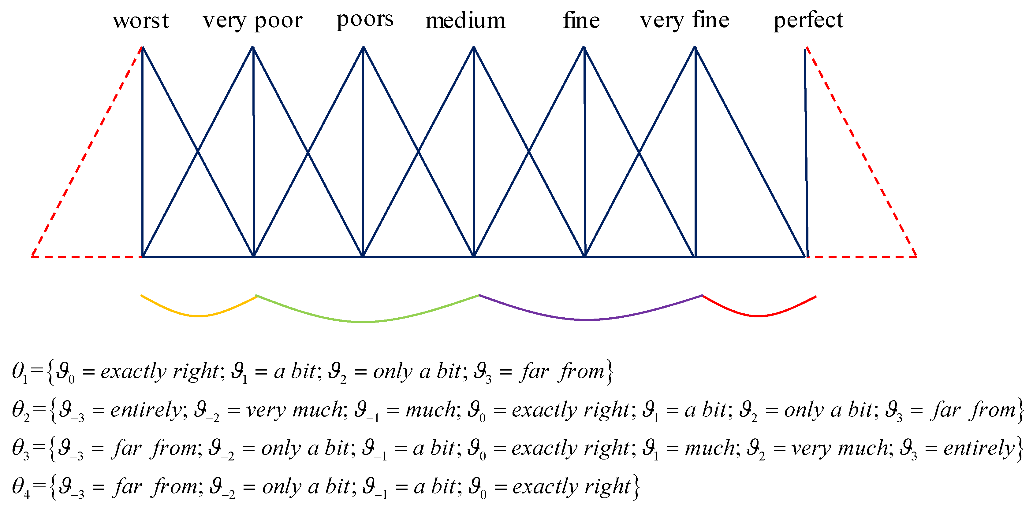
The DHHFLTS is made up of two hierarchy LTSs, in which the SHLTS indicates a further explanation or elaborate presentation of a given LT contained in the first hierarchy LTS. In other words, several buttons are installed to the LT contained in the first hierarchy LTS to depict its true extent. Therefore, compared with HFLTS, the DHHFLTS can express information more comprehensively and accurately. For instance, when the DMs want to express their view “Between far from poor and much fine”, it is more precise to use the DHHFLTS { ς - 1 < ϑ 3 > , ς 0 , ς 1 < ϑ 1 > } than the HFLTS { ς 1 , ς 0 , ς 1 } . Obviously, the DHHFLTS can depict the DM’s complex cognition and information more accurately.
(2)
The proposed operators take the support degree between any two inputs into consideration. When the evaluation value of alternatives under a certain attribute is closer, the attribute should be given a greater weight. Hence, the approaches can weaken the impact of unjustified extremum on the aggregation results. Additionally, the newly proposed operators are related to the parameter η , which is given by the DMs on account of the extent of their adventure appetite. Nonetheless the HFLWA and HFLWG operators with the absence of any parameter thus fail to imitate the DM’s adventure preference. For the sake of further showing this advantage of proposed method, an example can be given as follows.
Remark 1.
Based on the normalized matrix H S θ , we can easily find out that there are fine distinction among the evaluation values of χ δ 1 under the four attributes, which are { ς 0 < ϑ - 1 > , ς 1 < ϑ 1 > } , { ς 0 < ϑ 2 > } , { ς 2 < ϑ 0 > , ς 2 < ϑ 1 > } , { ς 1 < ϑ 2 > , ς 1 < ϑ 3 > } . Therefore, we can only change the attribute value H S θ 14 from { ς 1 < ϑ 2 > , ς 1 < ϑ 3 > } to the maximal value { ς 3 < ϑ 0 > , ς 1 < ϑ 3 > } . The corresponding ranking result are present in Table 7.
From Table 7, it is easy to find out that the expected and score values of alternative χ δ 1 for two operators are both becoming higher with the increase of the value of the beneficial attribute. Nevertheless, the ranking result remains unchanged by the proposed method, while it is changed by the method proposed by Zhang. This can justify the strength of the proposed approach in relieving the effect of extreme values.

5.4. Availability Verification

Next, we will further verify the availability of the newly presented approach from the perspective of the approach itself. Wang et al. indicated that an effective MADM approach requires to meet the following three standards,
Standard 1 (Optimality), In the case of the weight vector of decision attribute remains the same, the optimum action remains unchanged when we replaced the action less than optimal with a more terrible one.
Standard 2 (Transitivity), If the alternative Z1 is superior to the alternative Z2, and the alternative Z2 is superior to the alternative Z3, then we can obtain Z1 is superior to Z3.
Standard 3 (Detachability), Suppose a MADM problem is split into several sub-issues and rank the alternatives of these sub-issues by the same MADM method, then the comprehensive ranking result ought to be in accordance with the initial sorting of the original problem.
Now, we will prove the validity of our newly-presented approach under the aforesaid standards respectively.
(1) Verification on Standard 1.
To prove the effectiveness under the Standard 1, we change the evaluation values of the suboptimal alternative ( χ δ 3 ) and the penultimate alternative ( χ δ 4 ) without changing the attribute weight, and the adjusted decision matrix H ˜ S θ is given as follows,
H ˜ S θ = [ { ς 0 < ϑ - 1 > , ς 1 < ϑ 1 > } { ς 0 < ϑ 2 > } { ς 2 < ϑ 0 > , ς 2 < ϑ 1 > } { ς 1 < ϑ 2 > , ς 1 < ϑ 3 > } { ς 0 < ϑ - 3 > , ς 1 < ϑ 1 > } { ς 1 < ϑ 3 > , ς 2 < ϑ 2 > } { ς 2 < ϑ 1 > , ς 2 < ϑ 2 > } { ς 3 < ϑ - 1 > } { ς 0 < ϑ - 2 > , ς 0 < ϑ - 1 > } { ς 1 < ϑ 1 > , ς 1 < ϑ 0 > } { ς 1 < ϑ 2 > } { ς 2 < ϑ 0 > , ς 2 < ϑ 2 > } { ς - 1 < ϑ - 2 > } { ς 2 < ϑ 1 > , ς 2 < ϑ 0 > } { ς 1 < ϑ 3 > , ς 2 < ϑ 2 > } { ς 2 < ϑ - 1 > , ς 2 < ϑ 0 > } ]
Then utilize our above-proposed approach to deal with the assessment values and sort the alternatives with η = 2 , and the results are present as below,
M e ( h s θ 1 ) = 0.97794 ; M e ( h s θ 2 ) = 0.999248 ; M e ( h s θ 3 ) = 0.985042 ; M e ( h s θ 4 ) = 0.988175.
Thus we get the new ranking result as χ δ 2 χ δ 4 χ δ 3 χ δ 1 . We can find out that the optimal alternative is still χ δ 2 , in other words, the worsening of the suboptimal alternative has no effect on the priority of the optimal alternative. Therefore, our proposed method is valid under the Standard 1.
(2) Verification on and Standard 2 and Standard 3.
To prove the validity under the Standard 2 and Standard 3, we divide the initial MADM method into three sub-problems with the alternatives { χ δ 3 , χ δ 4 } , { χ δ 2 , χ δ 3 } , { χ δ 1 , χ δ 4 } , { χ δ 2 , χ δ 4 } , { χ δ 1 , χ δ 3 } and { χ δ 1 , χ δ 2 } . On the basis of the decision procedure of newly proposed approach, the ranking results of sub-issues are χ δ 3 χ δ 4 , χ δ 2 χ δ 3 , χ δ 4 χ δ 1 , χ δ 2 χ δ 4 , χ δ 3 χ δ 1 and χ δ 2 χ δ 1 . Then we combined these ranking result into the comprehensive ranking χ δ 2 χ δ 3 χ δ 4 χ δ 1 , which is the initial ranking result before splitting. Accordingly, our presented approach is in accord with the Standard 2 and Standard 3.
In conclusion, the proposed method satisfies all of the three validity standards, which proves that the method is effective.

6. Conclusions

For the sake of combining the strength of GPA operator and DHHFLTS, in this thesis, we have defined four novel operators, such as the DHHFLGPA, DHHFLGPG, DHHFLWGPA and DHHFLWGPG operators. Then several attractive properties, as well as representative cases of such operators, are demonstrated. On the basis of newly-presented operators, an effective approach is introduced to handle MADM problems under DHHFL environment. The strengths of presented operators and the novel decision-making method have been verified via a comparison analysis. Finally, according to three standards present by Wang and Triantaphyllou [40], we have justified the availability of the proposed approach.
Our proposed method has the following advantages: On one hand, for the DMs, they can express their views among the performance of alternatives more clearly and accurately by using DHHFLEs. In addition, the parameter η can be given according to their levels of risk appetite. On the other hand, taking the support degree into account, the proposed approach can weaken the impact of unjustified extremum on the aggregation results, which makes the decision results more reasonable and effective. Therefore, our research is meaningful and worthy of further expansion and application.
In further research, we will extend some MADM approaches to the DHHFL environment, such as TOPSIS, TODIM and GRA, to fully combine the characteristics of approaches themselves and the linguistic dominance of DHHFLTS. In addition, there is an embryonic project to ameliorate the proposed approach to handle incomplete weight information by combining various weight processing methods. Moreover, we will further apply the proposed method to other research domains, such as big data analysis, comprehensive ecological improvement, project management, and collaborative logistics networks [41], etc.

Author Contributions

Conceptualization, P.L.; Funding acquisition, Z.L.; Methodology, X.Z. and D.W.; Supervision, P.L.; Validation, D.W.; Writing–original draft, X.Z.; Writing–review & editing, Z.L.

Funding

This study was funded by the Social Sciences Research Project of Ministry of Education of China (No. 17YJA630065), the Shandong Provincial Natural Science Foundation, China (No.ZR2017MG007), the Project of Shandong Province Higher Educational Science and Technology Program(No. J16LN25) and the Special Funds of Taishan Scholars Project of Shandong Province (No. ts201511045).

Conflicts of Interest

The authors declare no conflict of interest.

References

  1. Nunić, Z. Evaluation and selection of Manufacturer PVC carpentry using FUCOM-MABAC model. ORESTA 2018, 1, 13–28. [Google Scholar] [CrossRef]
  2. Liu, Z.; Wang, S.; Liu, P. Multiple attribute group decision making based on q-rung orthopair fuzzy Heronian mean operators. Int. J. Intell. Syst. 2018, 33, 2341–2363. [Google Scholar] [CrossRef]
  3. Pamučar, D.; Lukovac, V.; Božanić, D.; Komazec, N. Multi-criteria FUCOM-MAIRCA model for the evaluation of level crossings, case study in the Republic of Serbia. ORESTA 2018, 1, 108–129. [Google Scholar] [CrossRef]
  4. Fazlollahtabar, H.; Smailbašić, A.; Stević, Ž. FUCOM method in group decision-making, Selection of forklift in a warehouse. Decis. Mak. Appl. Manag. Eng. 2019, 2, 49–65. [Google Scholar] [CrossRef]
  5. Vesković, S.; Stević, Ž.; Stojić, G.; Vasiljević, M.; Milinković, S. Evaluation of the railway management model by using a new integrated model DELPHI-SWARA-MABAC. Decis. Mak. Appl. Manag. Eng. 2018, 1, 34–50. [Google Scholar] [CrossRef]
  6. Karabasevic, D.; Popovic, G.; Stanujkic, D.; Maksimovic, M.; Sava, C. An approach for hotel type selection based on the single-valued intuitionistic fuzzy numbers. CO Publ. 2019, 1–2, 7. [Google Scholar]
  7. Liu, Z.; Li, L.; Li, J. q-Rung orthopair uncertain linguistic partitioned Bonferroni mean operators and its application to multiple attribute decision-making method. Int. J. Intell. Syst. 2019, 34, 2490–2520. [Google Scholar] [CrossRef]
  8. Liu, Z.; Liu, P.; Liang, X. Multiple attribute decision-making method for dealing with heterogeneous relationship among attributes and unknown attribute weight information under q-rung orthopair fuzzy environment. Int. J. Intell. Syst. 2018, 33, 1900–1928. [Google Scholar] [CrossRef]
  9. Levrat, E.; Voisin, A.; Bombardier, S. Subjective evaluation of car seat comfort with fuzzy set techniques. Int. J. Intell. Syst. 1997, 12, 891–913. [Google Scholar] [CrossRef]
  10. Zadeh, L.A. The concept of a linguistic variable and its application to approximate reasoning—I. Inf. Sci. 1975, 8, 199–249. [Google Scholar] [CrossRef]
  11. Mizumoto, M.; Tanaka, K. Some properties of fuzzy sets of type 2. Inf. Control 1976, 31, 312–340. [Google Scholar] [CrossRef] [Green Version]
  12. Martinez, L.; Herrera, F. An overview on the 2-tuple linguistic model for computing with words in decision making, Extensions, applications and challenges. Inf. Sci. 2012, 207, 1–18. [Google Scholar] [CrossRef]
  13. Rodriguez, R.M.; Martinez, L.; Herrera, F. Hesitant fuzzy linguistic term sets for decision making. IEEE Trans. Fuzzy Syst. 2012, 20, 109–119. [Google Scholar] [CrossRef]
  14. Gou, X.; Liao, H.; Xu, Z. Double hierarchy hesitant fuzzy linguistic term set and MULTIMOORA method, A case of study to evaluate the implementation status of haze controlling measures. Inf. Fusion 2017, 38, 22–34. [Google Scholar] [CrossRef]
  15. Liao, H.; Xu, Z.; Zeng, X.J. Distance and similarity measures for hesitant fuzzy linguistic termets and their application in multi-criteria decision making. Inf. Sci. 2014, 271, 125–142. [Google Scholar] [CrossRef]
  16. Torra, V. Hesitant fuzzy sets. Int. J. Intell. Syst. 2010, 25, 529–539. [Google Scholar] [CrossRef]
  17. Liao, H.; Xu, Z.; Herrera-Viedma, E.; Herrera, F. Hesitant fuzzy linguistic term set and its application in decision making, a state-of-the-art survey. Int. J. Fuzzy Syst. 2018, 20, 2084–2110. [Google Scholar] [CrossRef]
  18. Gou, X.; Xu, Z.; Liao, H. Multiple criteria decision making based on Bonferroni means with hesitant fuzzy linguistic information. Soft Comput. 2017, 21, 6515–6529. [Google Scholar] [CrossRef]
  19. Zhang, Z.; Wu, C. On the use of multiplicative consistency in hesitant fuzzy linguistic preference relations. Knowl. Based Syst. 2014, 72, 13–27. [Google Scholar] [CrossRef]
  20. Wang, J.; Wang, J.; Chen, Q. An outranking approach for multi-criteria decision-making with hesitant fuzzy linguistic term sets. Inf. Sci. 2014, 280, 338–351. [Google Scholar] [CrossRef]
  21. Liao, H.; Gou, X.; Xu, Z.; Zeng, X.J.; Herrera, F. Hesitancy degree-based correlation measures for hesitant fuzzy linguistic term sets and their applications in multiple criteria decision making. Inf. Sci. 2020, 508, 275–292. [Google Scholar] [CrossRef]
  22. Gou, X.; Xu, Z.; Liao, H. Multiple criteria decision making based on distance and similarity measures under double hierarchy hesitant fuzzy linguistic environment. Comput. Ind. Eng. 2018, 126, 516–530. [Google Scholar] [CrossRef]
  23. Gou, X.; Xu, Z.; Herrera, F. Consensus reaching process for large-scale group decision making with double hierarchy hesitant fuzzy linguistic preference relations. Knowl. Based Syst. 2018, 157, 20–33. [Google Scholar] [CrossRef]
  24. Liu, X.; Wang, X.; Qu, Q. Double Hierarchy Hesitant Fuzzy Linguistic Mathematical Programming Method for MAGDM Based on Shapley Values and Incomplete Preference Information. IEEE Access 2018, 6, 74162–74179. [Google Scholar] [CrossRef]
  25. Krishankmar, R.; Subrajaa, L.S.; Ravichandran, K.S.A. Framework for Multi-Attribute Group Decision-Making Using Double Hierarchy Hesitant Fuzzy Linguistic Term Set. Int. J. Fuzzy Syst. 2019, 21, 1130–1143. [Google Scholar] [CrossRef]
  26. Wang, J.; Lu, J.P.; Wei, G.; Lin, R.; Wei, C. Models for MADM with Single-Valued Neutrosophic 2-Tuple Linguistic Muirhead Mean Operators. Mathematics 2019, 7, 442. [Google Scholar] [CrossRef]
  27. He, J.H.; Wang, X.D.; Zhang, R.T.; Li, L. Some q-Rung Picture Fuzzy Dombi Hamy Mean Operators with Their Application to Project Assessment. Mathematics 2019, 7, 468. [Google Scholar] [CrossRef]
  28. Liu, Z.; Liu, P. Intuitionistic uncertain linguistic partitioned Bonferroni means and their application to multiple attribute decision-making. Int. J. Syst. Sci. 2017, 48, 1092–1105. [Google Scholar] [CrossRef]
  29. Harsanyi, J.C.; Cardinal, W. Individualistic ethics, and interpersonal comparisons of utility. J. Political Econ. 1955, 63, 309–321. [Google Scholar] [CrossRef]
  30. Yager, R.R. On ordered weighted averaging aggregation operators in multi-criteria decision making. IEEE Trans. Syst. Man Cybern. 1988, 18, 183–190. [Google Scholar] [CrossRef]
  31. Beliakov, G.; Pradera, A.; Calvo, T. Aggregation Functions, A Guide for Practitioners; Springer: Heidelberg, Germany, 2007. [Google Scholar]
  32. Bonferroni, C. Sulle medie multiple di potenze. Boll. Dell’unione Mat. Ital. 1950, 5, 267–270. [Google Scholar]
  33. Yager, R.R. The power average operator. IEEE Trans. Syst. Man Cybern. A 2001, 31, 724–731. [Google Scholar] [CrossRef]
  34. Zhou, L.; Chen, H.; Liu, J. Generalized power aggregation operators and their applications in group decision making. Comput. Ind. Eng. 2012, 62, 989–999. [Google Scholar] [CrossRef]
  35. Liu, P.; Wang, Y. Multiple attribute group decision making methods based on intuitionistic linguistic power generalized aggregation operators. Appl. Soft Comput. 2014, 17, 90–104. [Google Scholar] [CrossRef]
  36. Liu, P.; Yu, X. 2-Dimension uncertain linguistic power generalized weighted aggregation operator and its application in multiple attribute group decision making. Knowl. Based Syst. 2014, 57, 69–80. [Google Scholar] [CrossRef]
  37. Liu, P.; Liu, Y. An approach to multiple attribute group decision making based on intuitionistic trapezoidal fuzzy power generalized aggregation operator. Int. J. Comput. Int. Syst. 2014, 7, 291–304. [Google Scholar] [CrossRef]
  38. Wu, Q.; Wu, P.; Zhou, Y. Some 2-tuple linguistic generalized power aggregation operators and their applications to multiple attribute group decision making. J. Intell. Fuzzy Syst. 2015, 29, 423–436. [Google Scholar] [CrossRef]
  39. Zhang, Z. Hesitant fuzzy power aggregation operators and their application to multiple attribute group decision making. Inf. Sci. 2013, 234, 150–181. [Google Scholar] [CrossRef]
  40. Wang, X.; Triantaphyllou, E. Ranking irregularities when evaluating alternatives by using some ELECTRE methods. Omega 2008, 36, 45–63. [Google Scholar] [CrossRef]
  41. Xu, X.; Hao, J.; Yu, L.; Deng, Y. Fuzzy Optimal Allocation Model for Task-Resource Assignment Problem in Collaborative Logistics Network. IEEE Trans. Fuzzy Syst. 2019, 27, 1112–1125. [Google Scholar] [CrossRef]
Figure 1. The allocations of four different forms of SHLTS.
Information 10 00339 g001
Table 1. Support degree of h s θ i 1 form h s θ i z .
S u p ( h s θ i 1 , h s θ i z ) z = 2 z = 3 z = 4
χ δ 1 0.25830.07220.3111
χ δ 2 0.19170.06110.2333
χ δ 3 0.18330.06390.2111
χ δ 4 0.10830.03330.1667
Table 2. Support degree of h s θ i 3 form h s θ i z .
S u p ( h s θ i 2 , h s θ i z ) z = 1 z = 3 z = 4
χ δ 1 0.17220.07500.3222
χ δ 2 0.12780.09720.3778
χ δ 3 0.12220.09720.3667
χ δ 4 0.07220.09720.3778
Table 3. Support degree of h s θ i 3 form h s θ i z .
S u p ( h s θ i 3 , h s θ i z ) z = 1 z = 2 z = 4
χ δ 1 0.14440.22500.3778
χ δ 2 0.12220.29170.3889
χ δ 3 0.12780.29170.3556
χ δ 4 0.06670.29170.3667
Table 4. Support degree of h s θ i 4 form h s θ i z .
S u p ( h s θ i 4 , h s θ i z ) z = 1 z = 2 z = 3
χ δ 1 0.15560.24170.0944
χ δ 2 0.11670.28330.0972
χ δ 3 0.10560.27500.0889
χ δ 4 0.08330.28330.0917
Table 5. The results under different values of η .
η Expected   Value M e ( h s θ i ) Ranking
η = 1 M e ( h s θ 1 ) = 0.994857 ; M e ( h s θ 2 ) = 0.999886 ; M e ( h s θ 3 ) = 0.998549 ; M e ( h s θ 4 ) = 0.998446. χ δ 2 χ δ 3 χ δ 4 χ δ 1
η = 2 M e ( h s θ 1 ) = 0.97794 ; M e ( h s θ 2 ) = 0.999248 ; M e ( h s θ 3 ) = 0.992484 ; M e ( h s θ 4 ) = 0.991994. χ δ 2 χ δ 3 χ δ 4 χ δ 1
η = 5 M e ( h s θ 1 ) = 0.925217 ; M e ( h s θ 2 ) = 0.995829 ; M e ( h s θ 3 ) = 0.970512 ; M e ( h s θ 4 ) = 0.969439 χ δ 2 χ δ 3 χ δ 4 χ δ 1
η = 7 M e ( h s θ 1 ) = 0.902284 ; M e ( h s θ 2 ) = 0.992726 ; M e ( h s θ 3 ) = 0.95742 ; M e ( h s θ 4 ) = 0.955059. χ δ 2 χ δ 3 χ δ 4 χ δ 1
η = 15 M e ( h s θ 1 ) = 0.864854 ; M e ( h s θ 2 ) = 0.981233 ; M e ( h s θ 3 ) = 0.926689 ; M e ( h s θ 4 ) = 0.920939. χ δ 2 χ δ 3 χ δ 4 χ δ 1
η = 23 M e ( h s θ 1 ) = 0.855485 ; M e ( h s θ 2 ) = 0.973321 ; M e ( h s θ 3 ) = 0.913584 ; M e ( h s θ 4 ) = 0.908138. χ δ 2 χ δ 3 χ δ 4 χ δ 1
η = 30 M e ( h s θ 1 ) = 0.853149 ; M e ( h s θ 2 ) = 0.968522 ; M e ( h s θ 3 ) = 0.907629 ; M e ( h s θ 4 ) = 0.903688. χ δ 2 χ δ 3 χ δ 4 χ δ 1
η = 46 M e ( h s θ 1 ) = 0.853018 ; M e ( h s θ 2 ) = 0.961603 ; M e ( h s θ 3 ) = 0.900954 ; M e ( h s θ 4 ) = 0.900858. χ δ 2 χ δ 3 χ δ 4 χ δ 1
η = 47 M e ( h s θ 1 ) = 0.853087 ; M e ( h s θ 2 ) = 0.96129 ; M e ( h s θ 3 ) = 0.900693 ; M e ( h s θ 4 ) = 0.90081. χ δ 2 χ δ 4 χ δ 3 χ δ 1
η = 55 M e ( h s θ 1 ) = 0.853709 ; M e ( h s θ 2 ) = 0.959111 ; M e ( h s θ 3 ) = 0.898955 ; M e ( h s θ 4 ) = 0.900632. χ δ 2 χ δ 4 χ δ 3 χ δ 1
Table 6. Ranking results obtained by different methods.
OperatorExpected/Score ValuesRanking
D H H F L W G P A M e ( h s θ 1 ) = 0.97794 ; M e ( h s θ 2 ) = 0.99925 ; M e ( h s θ 3 ) = 0.99248 ; M e ( h s θ 4 ) = 0.99199. χ δ 2 χ δ 3 χ δ 4 χ δ 1
H F L W A S ( h s θ 1 ) = 3.7 ; S ( h s θ 2 ) = 4.85 ; S ( h s θ 3 ) = 4.1 ; S ( h s θ 4 ) = 4.15. χ δ 2 χ δ 4 χ δ 3 χ δ 1
D H H F L W G P G M e ( h s θ 1 ) = 0.43645 ; M e ( h s θ 2 ) = 0.54699 ; M e ( h s θ 3 ) = 0.41843 ; M e ( h s θ 4 ) = 0.27345. χ δ 2 χ δ 1 χ δ 3 χ δ 4
H F L W G S ( h s θ 1 ) = 3.64716 ; S ( h s θ 2 ) = 4.65486 ; S ( h s θ 3 ) = 3.96811 ; S ( h s θ 4 ) = 3.58391. χ δ 2 χ δ 3 χ δ 1 χ δ 4
Table 7. The results obtained from different operators.
OperatorsExpected/Score ValuesRanking
D H H F L W G P A M e ( h s θ 1 ) = 0.99109 ; M e ( h s θ 2 ) = 0.99925 ; M e ( h s θ 3 ) = 0.99248 ; M e ( h s θ 4 ) = 0.99199. χ δ 2 χ δ 3 χ δ 4 χ δ 1
H F L W A S ( h s θ 1 ) = 4.1 ; S ( h s θ 2 ) = 4.85 ; S ( h s θ 3 ) = 4.1 ; S ( h s θ 4 ) = 4.15. χ δ 2 χ δ 4 χ δ 3 χ δ 1

