Optimal Resource Allocation to Reduce an Epidemic Spread and Its Complication ^†

Abstract

Mathematical modeling represents a useful instrument to describe epidemic spread and to propose useful control actions, such as vaccination scheduling, quarantine, informative campaign, and therapy, especially in the realistic hypothesis of resources limitations. Moreover, the same representation could efficiently describe different epidemic scenarios, involving, for example, computer viruses spreading in the network. In this paper, a new model describing an infectious disease and a possible complication is proposed; after deep-model analysis discussing the role of the reproduction number, an optimal control problem is formulated and solved to reduce the number of dead patients, minimizing the control effort. The results show the reasonability of the proposed model and the effectiveness of the control action, aiming at an efficient resource allocation; the model also describes the different reactions of a population with respect to an epidemic disease depending on the economic and social original conditions. The optimal control theory applied to the proposed new epidemic model provides a sensible reduction in the number of dead patients, also suggesting the suitable scheduling of the vaccination control. Future work will be devoted to the identification of the model parameters referring to specific epidemic disease and complications, also taking into account the geographic and social scenario.

1. Introduction

In the last few years, the importance of epidemic modeling and control has increased in respect of their capability to describe infectious disease and proposing suitable control strategies [1,2,3,4,5,6,7,8]; moreover, the power of epidemic modeling has been used also in different fields, such as to study the propagation effects of a virus outbreak on a network [9,10].

The scenario discussed in this paper considers a unique population in which an epidemic disease is spreading and a second non-infectious disease is present. The non-infectious disease is assumed not to be risky by itself, but it may be fatal when it becomes a complication of the epidemic disease. Moreover, while the former yields an immunity, the latter could be caught repeatedly. This is a very common scenario, and happens, for example, in measles and for the HIV/AIDS; if one thinks of an age-structured model, a similar context occurs if referring to elderly subjects who could be at risk when a complication is added to an infectious disease. This is the reason vaccination campaigns are promoted especially among subjects in risky conditions.

The problem of controlling two epidemic spreads has been considered in different control frameworks, depending on the specificity of the diseases considered and, in particular, on the modalities of contagiousness. A different point of view considers a unique epidemic disease and two distinct but interacting populations, such as in [11], or as in [12], where a disease spreading among two populations in interconnected regions is considered. It is shown that when there is only a partial immunization, the best treatment action is to preferentially control the region with the lower level of infection and only when there are resources left over it is advisable to treat the other population. In [13] the interaction between two different diseases, tuberculosis and diabetes mellitus, is discussed, noting that from a medical point of view diabetes mellitus is a risk factor for tuberculosis, and even that the latter may be caused by diabetes. Also, social and economic aspects are discussed, demonstrating that malnutrition, HIV, crowded living conditions and low level of standards in hospitals contribute to high incidence of tuberculosis. The influence of one disease on the spread of the second is discussed in [14], in which a complex pattern of epidemiological behavior is proposed. More than one complication, with respect to the main disease, is considered in [15], where typhoid fever is modeled and many complications are considered, along with data about the population.

Suitable strategies are introduced for trying to stop the epidemic spread; general possibilities are vaccination, whenever possible, informative campaigns, quarantine, and therapy. More ad hoc actions depend on specific disease, as in [2], where the most effective control is to improve the test to check for HIV. Optimal control appears to be the natural framework to face an epidemic disease with the best resource allocation [4,5,16,17,18].

In this paper, an improvement of the model introduced in [19] is proposed. A unique population with two pathologies is considered: the first one is the dangerous disease that may be transmitted only by contact with infected patients, and the second one may be fatal only if it becomes a complication of the first. Moreover, the former yields an immunity, whereas the second one could be caught repeatedly. The healthy population is partitioned into two classes—the subjects that can caught both the pathologies, and the ones that have the immunity from the first contagious epidemic. Then, there are three classes of patients: the first one of subjects with only the dangerous contagious disease; the second class constituted of patients with both pathologies; then there is the class of individuals that has the second disease and could caught also the first one, if not immunized.

Spontaneous healing is assumed as well as different birth and death rates for each class; this is the first difference with respect to the model in [19], in which it was not considered that a patient with the infectious disease could become healthy again without an external action. The second novelty is the deep-model analysis conducted to determine the existence of the equilibrium points and to discuss their stability; the presence of a bifurcation value for the contagious rate, as well as its relationship with the reproduction number, has been established. The two-epidemics model is controlled by using an optimal control strategy that involves the vaccination and the therapy of infected patients, in the realistic case of bounded resources; the introduction of these constraints represents a further novelty with respect to the model in [19]; in the numerical section, these aspects are discussed. The paper is organized as follows: in Section 2 the mathematical model proposed is discussed, whereas the optimal control problem formulation is introduced in Section 3. Numerical simulations and discussions are proposed in Section 4, and conclusions are in Section 5.

2. The Mathematical Model

The mathematical model proposed and discussed in this section describes the interactions between subjects in a population where two different diseases are present. The most dangerous one is an infectious disease; the other one is a complication that is a not particularly risky pathology when it is the only one affecting the patients, but it may become fatal in combination with the infectious one. Typical examples are HIV or pneumonia that weaken a patient that, consequently, may become vulnerable to other diseases that, in general, are not so dangerous. This is also what happens to the elderly population that is sensibly monitored and invited by the government to participate to vaccination campaigns, especially to avoid complications. Another example involves immunosuppressed subjects and measles; it becomes a risky disease essentially because of possible and frequent complications, such as diarrhea and pneumonia.

For an infectious disease, the basic model is the SIR one, considering the classical categories of susceptible (S), infected (I), and removed (R) subjects; in this case, a susceptible individual can catch the disease, thus becoming infectious, and then enters the class of removed people, having received the immunization; the latter can also be obtained with a vaccination action. If a second non-infectious disease is present in the population, the complete model must include other classes taking into account the main characteristics of this second illness; in particular, a subject does not get immunization from the complication. The infected patients can be divided according to two possible conditions, depending on whether they are or are not affected by the second pathology. Moreover, the possibility of being affected by the second pathology for susceptible subjects requires the introduction of a further class for the patients with the second pathology, but not still immune from the epidemic disease. Then, five states are introduced:

$x_1$: 

the individuals than can be infected by the contagious illness;

$x_2$: 

the individuals immune from the contagious illness;

$x_3$: 

the patients infected but not affected by the second pathology;

$x_4$: 

the patients affected by both the pathologies;

$x_5$: 

the patients affected by the second pathology only, not immune from the infectious illness.

Some hypotheses are assumed:

• individuals $x_1$ and $x_2$ can become affected by the second pathology;
• from the $x_5$ class it is possible to become an $x_1$ subject with probability $ϵ$ or, if already immunized, go in the $x_2$ class;
• a subject in the $x_1$ class can get the infectious disease from the $x_3$ and the $x_4$ subjects and enter in the $x_3$ class; successively, a subject could get also the second disease and transit in the $x_4$ class.

The main control action, the vaccination applied on susceptible subjects $x_1$, has already been mentioned; also, therapy actions over patients in the classes $x_3$, $x_4$, $x_5$ are introduced. More precisely, four control actions are considered:

$u_1$ 

represents the action devoted to vaccinating healthy non-immune individuals $x_1$, making them transition to the $x_2$;

$u_2$ 

is the therapy action over the patients in $x_3$;

$u_3$ 

is the therapy action over the patients in $x_4$;

$u_4$ 

the therapy for the second illness, applied to $x_5$.

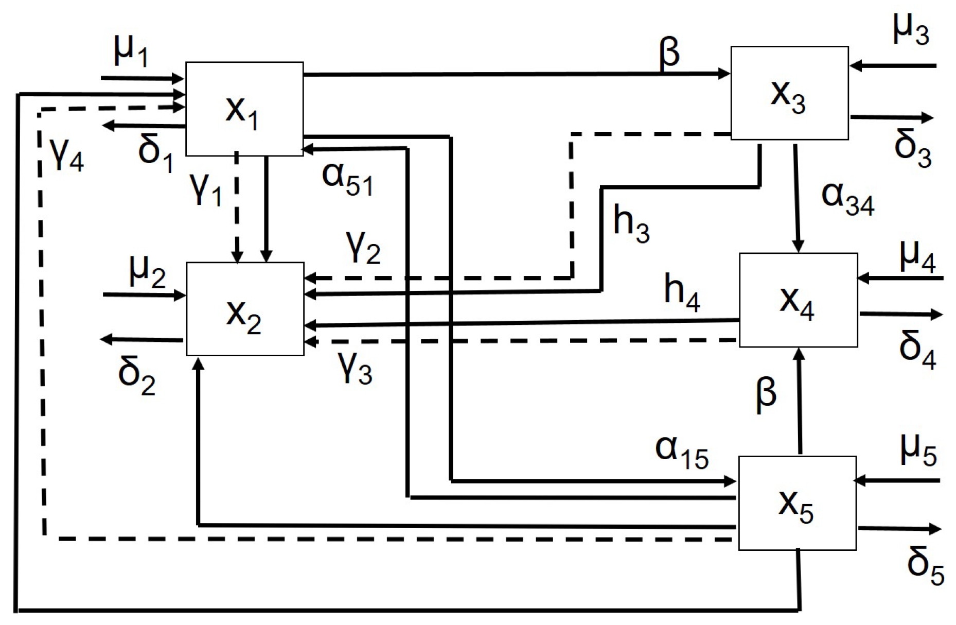
Defining $X={\left(\begin{array}{ccccc}{x}_1& x_2& x_3& x_4& x_5\end{array}\right)}^T$ the state vector and with $U={\left(\begin{array}{cccc}{u}_1& u_2& u_3& u_4\end{array}\right)}^T$ the control vector, the following model, shown in Figure 1, is proposed:

$$\dot{X}=F\left(X\right)+G\left(X\right)U$$

(1)

where:

$$F=\left(\begin{array}{c}{f}_1\\ f_2\\ f_3\\ f_4\\ f_5\end{array}\right)=\left(\begin{array}{c}-\beta x_1{x}_3-\beta x_1{x}_4-{\alpha }_{15}{x}_1+ϵ{\alpha }_{51}{x}_5-{\delta }_1{x}_1+{\mu }_1\\ (1-ϵ){\alpha }_{51}{x}_5-{\alpha }_{25}{x}_2-{\delta }_2{x}_2+{\mu }_2+h_3{x}_3+h_4{x}_4\\ \beta x_1{x}_3+\beta x_1{x}_4-{\alpha }_{34}{x}_3-{\delta }_3{x}_3+{\mu }_3-h_3{x}_3\\ {\alpha }_{34}{x}_3+\beta x_4{x}_5+\beta x_3{x}_5-{\delta }_4{x}_4+{\mu }_4-h_4{x}_4\\ {\alpha }_{15}{x}_1-{\alpha }_{51}{x}_5-\beta x_4{x}_5-\beta x_3{x}_5-{\delta }_5{x}_5+{\mu }_5+{\alpha }_{25}{x}_2\end{array}\right)$$

(2)

and

$$G=\left(\begin{array}{cccc}-{\gamma }_1{x}_1& 0& 0& {\gamma }_4{x}_5\\ {\gamma }_1{x}_1& {\gamma }_2{x}_3& {\gamma }_3{x}_4& 0\\ 0& -{\gamma }_2{x}_3& 0& 0\\ 0& 0& -{\gamma }_3{x}_4& 0\\ 0& 0& 0& -{\gamma }_4{x}_5\end{array}\right)$$

(3)

with initial condition $X\left(t_0\right)=X_0$. In the model (1), with (2) and (3), the parameters introduced are:

• $\beta$, the contagious rate;
• ${\alpha }_{ij}$, which are the occurrence rates of the second non-infectious pathology; the subscripts denote the transition from state i to state j; these rates can be assumed to be different, to put in evidence the differences between healthy people and infected ones. It is assumed that recovery from the second illness can also be spontaneous from the $x_5$ class, and the rate of autonomous healing is denoted again with the coefficients ${\alpha }_{51}$, being a natural transition proportional to the number of subjects;
• ${\gamma }_i$, $i=1,\dots ,4$ representing the efficiencies of the control actions;
• $h_j$, $j=3,4$, representing the spontaneous healing rate of the $x_3$ and $x_4$ patients respectively;
• ${\mu }_i$, $i=1,\dots ,5$, the rate of new incomers in all the compartments;
• ${\delta }_i$, $i=1,\dots ,5$, which are the percentages of removed people;
• $ϵ$, the percentage of subjects that from the $x_5$ class enter in the $x_1$ one.

This model represents an improvement of the one proposed in [19], in which the spontaneous healing capability was not included.

2.1. The Model Analysis

The analysis of the model is proposed, referring to the absence of control action as well as assuming no entries in the $x_3$, $x_4$, and $x_5$ compartments, thus ${\mu }_3={\mu }_4={\mu }_5=0$ in (1). To determine the equilibrium points the equation

$$\begin{array}{c}\hfill F\left(X\right)=0\end{array}$$

(4)

is considered, thus obtaining the system:

$$\begin{array}{c}\hfill -\beta x_1{x}_3-\beta x_1{x}_4-{\alpha }_{15}{x}_1+ϵ{\alpha }_{51}{x}_5-{\delta }_1{x}_1+{\mu }_1=0\end{array}$$

(5)

$$\begin{array}{c}\hfill (1-ϵ){\alpha }_{51}{x}_5-{\alpha }_{25}{x}_2-{\delta }_2{x}_2+{\mu }_2+h_3{x}_3+h_4{x}_4=0\end{array}$$

(6)

$$\begin{array}{c}\hfill \beta x_1{x}_3+\beta x_1{x}_4-{\alpha }_{34}{x}_3-{\delta }_3{x}_3-h_3{x}_3=0\end{array}$$

(7)

$$\begin{array}{c}\hfill {\alpha }_{34}{x}_3+\beta x_4{x}_5+\beta x_3{x}_5-{\delta }_4{x}_4-h_4{x}_4=0\end{array}$$

(8)

$$\begin{array}{c}\hfill {\alpha }_{15}{x}_1-{\alpha }_{51}{x}_5-\beta x_4{x}_5-\beta x_3{x}_5-{\delta }_5{x}_5+{\alpha }_{25}{x}_2=0\end{array}$$

(9)

One solution is the virus-free equilibrium

$$P_{e1}=\left(\begin{array}{c}\frac{({\alpha }_{25}{\delta }_5+{\alpha }_{51}{\delta }_2+{\delta }_2{\delta }_5+{\alpha }_{25}{\alpha }_{51}ϵ){\mu }_1+{\alpha }_{25}{\alpha }_{51}ϵ{\mu }_2}{{\alpha }_{15}{\delta }_5({\alpha }_{25}+{\delta }_2)+(1-ϵ){\alpha }_{15}{\alpha }_{51}{\delta }_2+{\alpha }_{25}{\delta }_1({\delta }_5+ϵ{\alpha }_{51})+{\delta }_1{\delta }_2({\alpha }_{51}+{\delta }_5)}\\ \frac{(1-ϵ){\alpha }_{15}{\alpha }_{51}({\mu }_1+{\mu }_2)+({\alpha }_{15}{\delta }_5+{\alpha }_{51}{\delta }_1+{\delta }_1{\delta }_2){\mu }_2}{{\alpha }_{15}{\delta }_5({\alpha }_{25}+{\delta }_2)+(1-ϵ){\alpha }_{15}{\alpha }_{51}{\delta }_2+{\alpha }_{25}{\delta }_1({\delta }_5+ϵ{\alpha }_{51})+{\delta }_1{\delta }_2({\alpha }_{51}+{\delta }_5)}\\ 0\\ 0\\ \frac{{\alpha }_{15}{\mu }_1({\alpha }_{25}+{\delta }_2)+{\alpha }_{25}{\mu }_2({\alpha }_{15}+{\delta }_1)}{{\alpha }_{15}{\delta }_5({\alpha }_{25}+{\delta }_2)+(1-ϵ){\alpha }_{15}{\alpha }_{51}{\delta }_2+{\alpha }_{25}{\delta }_1({\delta }_5+ϵ{\alpha }_{51})+{\delta }_1{\delta }_2({\alpha }_{51}+{\delta }_5)}\end{array}\right)$$

(10)

Please note that the non-null elements do not depend on $\beta$ and are positive for any combination of parameters; therefore, the point $P_{e1}$ in (10) is always an equilibrium point.

With regard to the other equilibrium points, the analytical solutions of the system (4) are rather complicated, and they depend also on $\beta$, in addition to all the other model parameters; the only acceptable points are those with non-negative components, if they exist. In the following, the model parameters, with the exception of $\beta$, are all fixed, thus deducing, from a graphical point of view, the dependence of the solutions of the system (5)–(9) on $\beta$. The following values of the parameters are used:

• ${\alpha }_{15}={\alpha }_{34}=0.1$
• ${\alpha }_{51}={\alpha }_{43}=0.05$
• ${\alpha }_{25}=0.01$
• ${\mu }_1={\mu }_2=10$
• ${\delta }_1={\delta }_2={\delta }_5=0.05$, ${\delta }_3=0.2$, ${\delta }_4=0.5$
• $ϵ=0.7$
• $h_3=h_4=0.01$

These choices have been guided by similarity with respect to classical epidemic models, such as the SIR one. By using these values, the system (5)–(9) has three solutions. They are not all feasible equilibrium points; the only acceptable solutions are those with all the components not negative. With these parameter values the virus-free equilibrium is:

$$P_{e1}={\left(\begin{array}{ccccc}76& 190& 0& 0& 95\end{array}\right)}^T$$

(11)

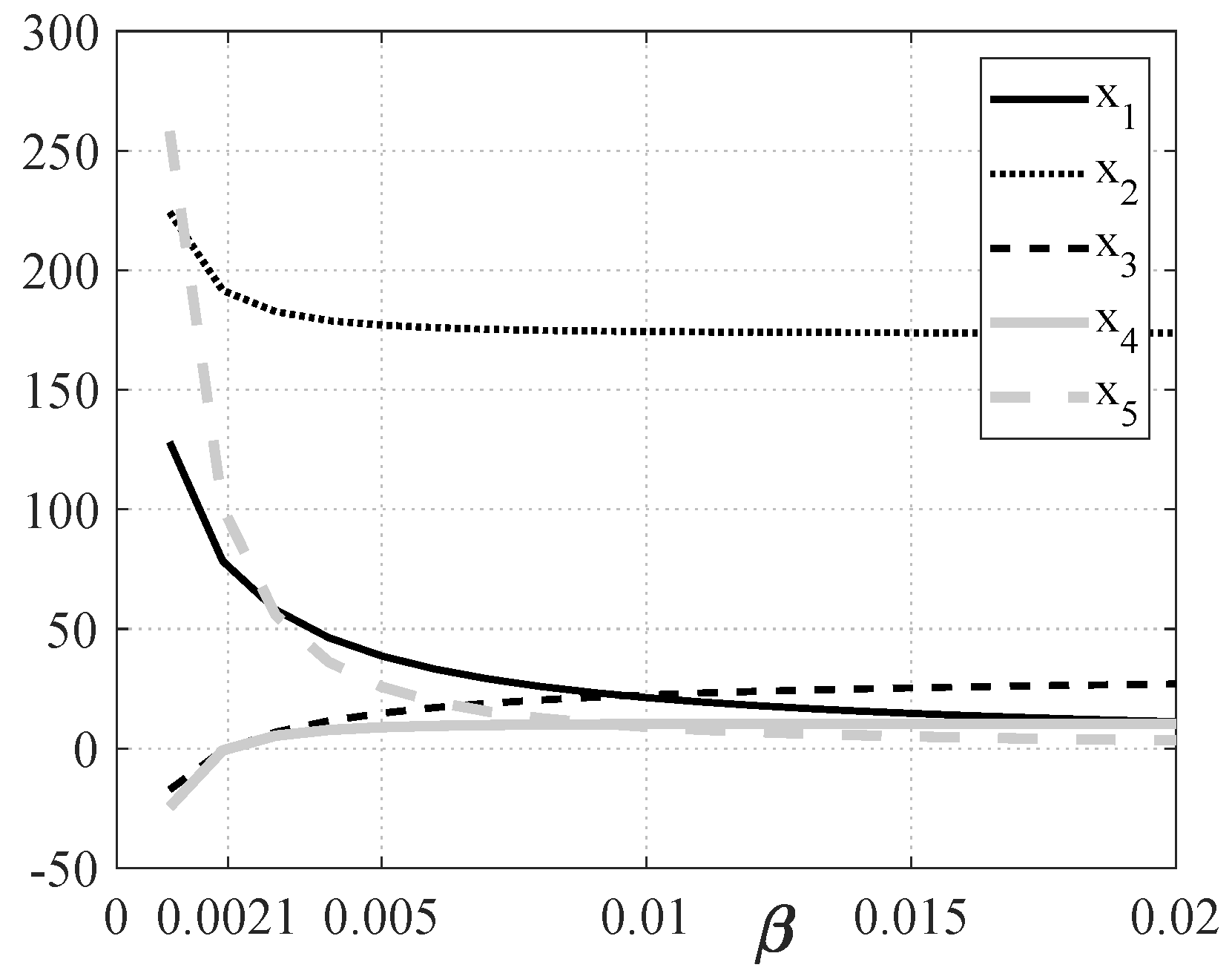
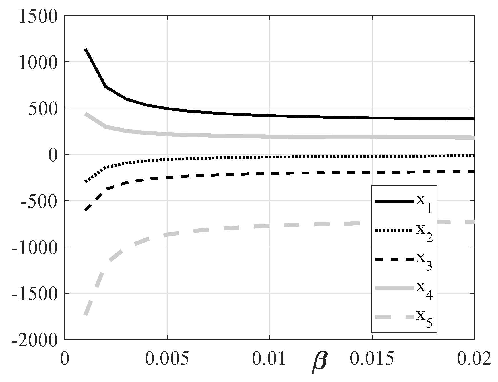
There are two other solutions of the system (5)–(9), called $P_2$ and $P_3$; in Figure 2 and Figure 3 they are shown as function of $\beta$, by plotting together the five components of each solution. It can be noted that in Figure 2 the component $x_4$ of the solution $P_2$ is negative up to a threshold value $\overline{\beta }$ of $\beta$, whereas from Figure 3 it can be observed that three components ($x_2$, $x_3$, and $x_5$) are always negative, and therefore $P_3$ is not an equilibrium point for any $\beta$. For a small contact rate $\beta <\overline{\beta }$, there exists only one equilibrium point, $P_{e1}$, whereas for $\beta >\overline{\beta }$ there exists also the second equilibrium point, now indicated by $P_{e2}$, whose components evolve as in Figure 2. The value of $\overline{\beta }$ corresponding to the chosen parameters is equal to $0.0021$, as can be deduced from Figure 2.

To study the stability of the equilibrium points, $P_{e1}$ and, if it exists, $P_{e2}$, the Jacobian of the system must be evaluated in each of these points and the corresponding eigenvalues calculated. The Jacobian is:

$$J=\left(\begin{array}{ccccc}-\beta (x_3+x_4)-\frac{3}{20}& 0& -\beta x_1& -\beta x_1& \frac{3}{200}\\ 0& -\frac{3}{50}& \frac{1}{100}& \frac{1}{100}& \frac{3}{200}\\ \beta (x_3+x_4)& 0& \beta x_1-\frac{31}{100}& \beta x_1& 0\\ 0& 0& \beta x_5+\frac{1}{10}& \beta x_5-\frac{51}{100}& \beta (x_3+x_4)\\ \frac{1}{10}& \frac{1}{100}& -\beta x_5& -\beta x_5& -\beta (x_3+x_4)-\frac{1}{10}\end{array}\right)$$

(12)

Obviously, the eigenvalues of the Jacobian matrix J depends on the value of $\beta$, once the components of the equilibrium point are substituted. Therefore, even if the virus-free equilibrium $P_{e1}$ components do not depend on $\beta$, as already noted, its stability does. The matrix (12), evaluated at $P_{e1}$, is

$$J\left(P_{e1}\right)=\left(\begin{array}{ccccc}-\frac{3}{20}& 0& -76\beta & -76\beta & \frac{3}{200}\\ 0& -\frac{3}{50}& \frac{1}{100}& \frac{1}{100}& \frac{3}{200}\\ 0& 0& 76\beta -\frac{31}{100}& 76\beta & 0\\ 0& 0& 95\beta +\frac{1}{10}& 95\beta -\frac{51}{100}& 0\\ \frac{1}{10}& \frac{1}{100}& -95\beta & -95\beta & -\frac{1}{10}\end{array}\right)$$

(13)

whose eigenvalues, as function of $\beta$, are:

$$\begin{array}{c}\hfill {\nu }_1=-0.0548{\nu }_2=-0.1714{\nu }_3=-0.0837\end{array}$$

(14)

$$\begin{array}{c}\hfill {\nu }_4=\frac{171\beta }{2}-\frac{41}{100}-\frac{\sqrt{731025{\beta }^2+570\beta +1}}{10}\end{array}$$

(15)

$$\begin{array}{c}\hfill {\nu }_5=\frac{171\beta }{2}-\frac{41}{100}+\frac{\sqrt{731025{\beta }^2+570\beta +1}}{10}\end{array}$$

(16)

The eigenvalues ${\nu }_1$, ${\nu }_2$, and ${\nu }_3$ are negative and do not depend on $\beta$; the eigenvalues ${\nu }_4$ and ${\nu }_5$ are negative only if $\beta <0.0021$, a value that coincides, as expected, with $\overline{\beta }$. It can be concluded that for $\beta <\overline{\beta }$ the unique equilibrium point $P_{e1}$ is locally asymptotically stable.

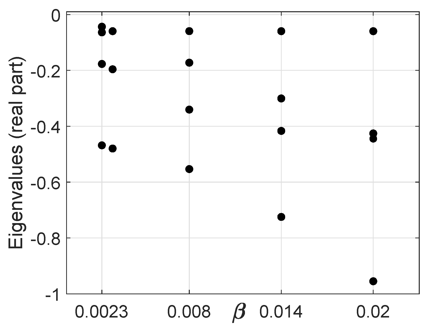
As for the second equilibrium point, $P_{e2}$, it has already been stated that it exists only for $\beta >0.0021$; the analysis of its stability is rather complicated from analytical point of view. In Figure 4 the real part of the eigenvalues of the Jacobian matrix J, Equation (12), when evaluated for some values of $\beta >\overline{\beta }$, $\beta =0.0023$, $0.003$, $0.008$, $0.014$, $0.02$ is shown. Please note that there exists a couple of complex eigenvalues with, as expected, the same real part.

Then, it is possible to conclude that for $\beta <\overline{\beta }$, $P_{e1}$ exists and is locally stable, while $P_2$ is not admissible; on the other hand, when $\beta >\overline{\beta }$, $P_{e1}$ is unstable while $P_2$ is a locally stable equilibrium point. This is the classical case of a Transcritical Bifurcation.

2.2. The Reproduction Number

The reproduction number $\mathcal{R}$, as recalled in [20] and [21], is a useful parameter to describe the capability of an infectious disease to invade a population. It is generally evaluated by using the next-generation matrix; more precisely, from the dynamical model (1), considering only the compartments of the subjects infected by the infectious disease, $x_3$ and $x_4$, the corresponding dynamical evolutions can be split into two parts, $M_3-N_3$ and $M_4-N_4$ respectively, collected in the two vectors:

$$M=\left(\begin{array}{c}\beta x_1(x_3+x_4)\\ \beta x_5(x_3+x_4)\end{array}\right)$$

(17)

$$N=\left(\begin{array}{c}{\alpha }_{34}{x}_3+{\delta }_3{x}_3+h_3{x}_3\\ {\delta }_4{x}_4+h_4{x}_4-{\alpha }_{34}{x}_3\end{array}\right)$$

(18)

The matrix (17) accounts for the rate of appearance of new infections in the compartments $x_3$ and $x_4$, whereas (18) describes the rate of other transitions between them. Now, the Jacobian of (17) and (18) is:

$$J_M=\left(\begin{array}{cc}\beta x_1& \beta x_1\\ \beta x_5& \beta x_5\end{array}\right)$$

$$J_N=\left(\begin{array}{cc}{\alpha }_{34}+{\delta }_3+h_3& 0\\ -{\alpha }_{34}& {\delta }_4+h_4\end{array}\right)$$

To evaluate the next-generation matrix, the matrix $J_M{J}_N^{-1}$ must be evaluated at the virus-free equilibrium (10), thus obtaining:

$$J_M{J}_N^{-1}=\left(\begin{array}{cc}0.63\beta x_1& 1.96\beta x_1\\ 3.86\beta x_5& 1.96\beta x_5\end{array}\right)$$

that is, by substituting the coordinates of (11);

$$J_M{J}_N^{-1}\left(P_{e1}\right)=\left(\begin{array}{cc}48.07\beta & 149\beta \\ 366.54\beta & 186.27\beta \end{array}\right)$$

The reproduction number is defined as the spectral radius of the matrix $J_M{J}_N^{-1}\left(P_{e1}\right)$, whose eigenvalues, as a function of $\beta$, are:

$$\begin{array}{c}\hfill {\lambda }_1=-126.54\beta {\lambda }_2=360.88\beta \end{array}$$

(19)

Therefore, the reproduction number for the proposed choice of parameters is $\mathcal{R}=360.88\beta$. By definition, if $\mathcal{R}=360.88\beta <1$, the infection cannot grow, whereas if $\mathcal{R}=360.88\beta >1$ the disease can spread over the population, [20]. The value of $\beta$ that separates these two situations is $\frac{1}{360.88}$ which coincides, obviously, with $\overline{\beta }$.

3. Formulation of the Optimal Control Problem

The problem of the containment of an epidemic spread could be efficiently solved by the framework of optimal control theory; in this case, particular attention is devoted to patients with the two pathologies. The optimal control approach suggests the best strategy to allocate the resources properly, distinguishing between the different level of illness. The necessity of containing the number of infected individuals and the cost of the intervention suggests the introduction of a cost index that weights both the number of infected individuals and the control cost. Moreover, it is assumed that the resources are bounded, in particular:

$$0\le u_i\left(t\right)\le U_i^M,i=1,\dots ,4$$

(20)

For the sake of notation, it is useful to write them as follows:

$$\begin{array}{c}\hfill q_1=-u_1\le 0q_2=u_1-u_1^M\le 0\end{array}$$

(21)

$$\begin{array}{c}\hfill q_3=-u_2\le 0q_4=u_2-u_2^M\le 0\end{array}$$

(22)

$$\begin{array}{c}\hfill q_5=-u_3\le 0q_6=u_3-u_3^M\le 0\end{array}$$

(23)

$$\begin{array}{c}\hfill q_7=-u_4\le 0q_8=u_4-u_4^M\le 0\end{array}$$

(24)

The classical quadratic structure

$$J=\frac{1}{2}{\int }_{t_0}^{t_f}\left(a_3{x}_3^2+a_4{x}_4^2+a_5{x}_5^2+r_1{u}_1^2+r_2{u}_2^2+r_3{u}_3^2+r_4{u}_4^2\right)dt$$

(25)

is chosen for the cost function, where $a_i$, $i=3,4,5$, and $r_i$, $i=1,\dots ,4$ are the weights of the state variables and the controls, respectively. The final time $t_f$ is fixed while the final state value is left free. From (1) and (25), the corresponding Hamiltonian is

$$\begin{array}{c}\hfill H=\frac{1}{2}\left(a_3{x}_3^2+a_4{x}_4^2+a_5{x}_5^2+r_1{u}_1^2+r_2{u}_2^2\right.\left.+r_3{u}_3^2+r_4{u}_4^2\right)\\ \hfill -{\lambda }_1\left(\beta x_1{x}_3\right.+\beta x_1{x}_4+{\alpha }_{15}{x}_1-{\alpha }_{51}{x}_5+{\gamma }_1{x}_1{u}_1\left.-{\gamma }_4{x}_5{u}_4+{\delta }_1{x}_1-{\mu }_1+ϵ{\alpha }_{51}{x}_5\right)\\ \hfill +{\lambda }_2\left({\gamma }_1{x}_1{u}_1\right.\left.+{\gamma }_2{x}_3{u}_2+{\gamma }_3{x}_4{u}_3-{\delta }_2{x}_2+{\mu }_2+(1-ϵ){\alpha }_{51}{x}_5-{\alpha }_{25}{x}_2+h_3{x}_3+h_4{x}_4\right)\\ \hfill +{\lambda }_3\left(\beta x_1{x}_3+\beta x_1{x}_4-{\alpha }_{34}{x}_3-{\gamma }_2{x}_3{u}_2\right.\left.-{\delta }_3{x}_3+{\mu }_3-h_3{x}_3\right)\\ \hfill +{\lambda }_4\left({\alpha }_{34}{x}_3+\beta x_4{x}_5\right.\left.+\beta x_3{x}_5-{\gamma }_3{x}_4{u}_3-{\delta }_4{x}_4+{\mu }_4-h_4{x}_4\right)\\ \hfill +{\lambda }_5\left({\alpha }_{15}{x}_1-{\alpha }_{51}{x}_5-\beta x_4{x}_5-\beta x_3{x}_5\right.\left.-{\gamma }_4{x}_5{u}_4-{\delta }_5{x}_5+{\mu }_5+{\alpha }_{25}{x}_2\right)\end{array}$$

(26)

The Hamiltonian function is constantly equal to zero along the optimal trajectories over the whole control interval, since the final time $t_f$ is fixed.

With the introduction of the costate vector $\lambda ={\left(\begin{array}{ccccc}{\lambda }_1\left(t\right)& {\lambda }_2\left(t\right))& {\lambda }_3\left(t\right)& {\lambda }_4\left(t\right)& {\lambda }_5\left(t\right)\end{array}\right)}^T$, and ${\eta }_i$, $i=1,2,\dots ,8$, real valued functions, the necessary conditions are:

$$\begin{array}{c}\hfill {\dot{\lambda }}_i=-\frac{\partial H}{\partial x_i},i=1,\dots ,5\end{array}$$

(27)

$$0=\frac{\partial H}{\partial u_j}+\sum _{k=1}^8\frac{\partial q_k}{\partial u_j}{\eta }_k,j=1,\dots ,4$$

(28)

$${\eta }_j{q}_j=0,j=1,\dots ,8$$

(29)

$${\eta }_j\ge 0,j=1,\dots ,8$$

(30)

with final conditions:

$${\lambda }_i\left(t_f\right)=0,i=1,\dots ,5$$

(31)

Please note that in (27) the independence of $q_j$, $j=1,\dots ,8$ from the state X has been used. The costate Equation (27) yields:

$$\begin{array}{ccc}\hfill {\dot{\lambda }}_1& =& \beta {\lambda }_1{x}_3+\beta {\lambda }_1{x}_4+{\alpha }_{15}{\lambda }_1+{\gamma }_1{\lambda }_1{u}_1+{\delta }_1{\lambda }_1-{\gamma }_1{\lambda }_2{u}_1-\beta {\lambda }_3{x}_3-\beta {\lambda }_3{x}_4-{\alpha }_{15}{\lambda }_5\hfill \end{array}$$

(32)

$$\begin{array}{ccc}\hfill {\dot{\lambda }}_2& =& {\delta }_2{\lambda }_2-{\lambda }_5{\alpha }_{25}\hfill \end{array}$$

(33)

$$\begin{array}{ccc}\hfill {\dot{\lambda }}_3& =& -a_3{x}_3+\beta x_1{\lambda }_1-{\gamma }_2{\lambda }_2{u}_2-{\lambda }_2{h}_3+{\lambda }_3{h}_3+\gamma \beta x_1{\lambda }_3+{\alpha }_{34}{\lambda }_3+{\gamma }_2{\lambda }_3{u}_2\hfill \\ & & +{\delta }_3{\lambda }_3-{\alpha }_{34}{\lambda }_4-\beta {\lambda }_4{x}_5+\beta {\lambda }_5{x}_5\hfill \end{array}$$

(34)

$$\begin{array}{ccc}\hfill {\dot{\lambda }}_4& =& -a_4{x}_4+\beta x_1{\lambda }_1-{\gamma }_3{\lambda }_2{u}_3-{\lambda }_2{h}_4-\beta x_1{\lambda }_3-\beta {\lambda }_4{x}_5+{\gamma }_3{\lambda }_4{u}_3\hfill \\ & & +{\delta }_4{\lambda }_4+{\lambda }_4{h}_4+\beta {\lambda }_5{x}_5\hfill \end{array}$$

(35)

$$\begin{array}{ccc}\hfill {\dot{\lambda }}_5& =& -a_5{x}_5-{\alpha }_{51}{\lambda }_1-{\gamma }_4{\lambda }_1{u}_4+{\lambda }_1ϵ{\alpha }_{51}{x}_5-{\lambda }_2(1-ϵ){\alpha }_{51}{x}_5-\beta x_4{\lambda }_4\hfill \\ & & -\beta x_3{\lambda }_4+{\alpha }_{51}{\lambda }_5+\beta x_4{\lambda }_5+\beta x_3{\lambda }_5+{\gamma }_4{\lambda }_5{u}_4+{\delta }_5{\lambda }_5\hfill \end{array}$$

(36)

for which ${\lambda }_i\left(t_f\right)=0$, $i=1,\dots ,5$, hold since $x\left(t_f\right)$ is not fixed. The control Equation (28) implies:

$$\begin{array}{ccc}\hfill 0& =& \frac{\partial H}{\partial u_1}+\frac{\partial q_1}{\partial u_1}{\eta }_1+\frac{\partial q_2}{\partial u_1}{\eta }_2=r_1{u}_1-{\gamma }_1{\lambda }_1{x}_1-{\eta }_1+{\eta }_2\hfill \end{array}$$

(37)

$$\begin{array}{ccc}\hfill 0& =& \frac{\partial H}{\partial u_2}+\frac{\partial q_3}{\partial u_2}{\eta }_3+\frac{\partial q_4}{\partial u_2}{\eta }_4=r_2{u}_2-{\gamma }_2{\lambda }_3{x}_3-{\eta }_3+{\eta }_4\hfill \end{array}$$

(38)

$$\begin{array}{ccc}\hfill 0& =& \frac{\partial H}{\partial u_3}+\frac{\partial q_5}{\partial u_3}{\eta }_5+\frac{\partial q_6}{\partial u_3}{\eta }_6=r_3{u}_3+{\gamma }_3{\lambda }_2{x}_4-{\gamma }_3{\lambda }_4{x}_4-{\eta }_5+{\eta }_6\hfill \end{array}$$

(39)

$$\begin{array}{ccc}\hfill 0& =& \frac{\partial H}{\partial u_4}+\frac{\partial q_7}{\partial u_4}{\eta }_7+\frac{\partial q_8}{\partial u_4}{\eta }_8=r_4{u}_4-{\gamma }_4{\lambda }_1{x}_5-{\gamma }_4{\lambda }_5{x}_5-{\eta }_7+{\eta }_8\hfill \end{array}$$

(40)

By taking into account the conditions (29) and (30), $2^8$ cases are possible, but they are reduced by eliminating the contrasting conditions. The control equations with conditions (29) and (30), along with the costate and the state equations, yield the expressions for the controls:

$$u_1=max\{min\{\frac{{\gamma }_1}{r_1}{\lambda }_1{x}_1,u_1^M\},0\}$$

(41)

$$u_2=max\{min\{\frac{{\gamma }_2}{r_2}{\lambda }_3{x}_2,u_2^M\},0\}$$

(42)

$$u_3=max\{min\{-\frac{{\gamma }_3}{r_3}\left({\lambda }_2-{\lambda }_4\right)x_4,u_3^M\},0\}$$

(43)

$$u_4=max\{min\{-\frac{{\gamma }_4}{r_4}\left({\lambda }_1-{\lambda }_5\right)x_5,u_4^M\},0\}$$

(44)

for which it is necessary to compute $X\left(t\right)$ and $\lambda \left(t\right)$, from $t=t_0$ to $t=t_f$, making use of Equation (1), to be integrated from the initial condition $X\left(t_0\right)=X_0$, and Equations (32)—(36) to be integrated backwards in time from ${\lambda }_i\left(t_f\right)=0$, $i=1,\dots ,5$.

4. Simulations Results

In this Section, the proposed model and the optimal control strategy are analyzed numerically. The algorithm adopted for the optimal control problem is based on a sequential quadratic programming method: at each iteration, a quadratic programming subproblem is solved by using a quasi-Newton approximation of the Hessian of the Lagrangian function. The parameters of the model are the ones proposed in Section 2; the initial conditions assumed reflect the situation in which the population is mostly composed of susceptible subjects and a small number of infected individuals: $x_1\left(0\right)=1000$, $x_2\left(0\right)=0$, $x_3\left(0\right)=10$, $x_4\left(0\right)=0$, and $x_5\left(0\right)=0$. The state terms $a_i{x}_i^2$ in the cost index can be interpreted as the number of dead individuals among the three groups of patients; the result is obtained by setting $a_i={\delta }_i^2$, $i=3,4,5$. The time control period is set equal to 5 years. To study the effectiveness of the model as well as the reasonability of the optimal control strategy, some case studies are proposed. To evaluate the advantages of the different strategies, some quantities are calculated:

• the variation V of the sum of the number of dead people in the classes $x_3$ and $x_4$, the ones in which the patients are more at risk, normalized with respect to the same quantity in absence of control;
• the cost $C_i$ of the control $u_i$, $i=1,\dots ,4$;
• the efficacy E of the control action measured as the product of the total number of dead people (in all the classes) multiplied by the total cost applied.

As Case 1, a first choice of the $\beta$ parameter is $\beta =0.001<\overline{\beta }$; this means that the epidemic will not spread, being the corresponding $\mathcal{R}=0.3609<1$. The same analysis is performed in Case 2 by choosing $\beta =0.01>\overline{\beta }$; the corresponding reproduction number is $\mathcal{R}=3.6088>1$ thus leading to an endemic condition. All the control weights in the cost function (25) are set equal to $r_1=r_2=r_3=r_4=10$.

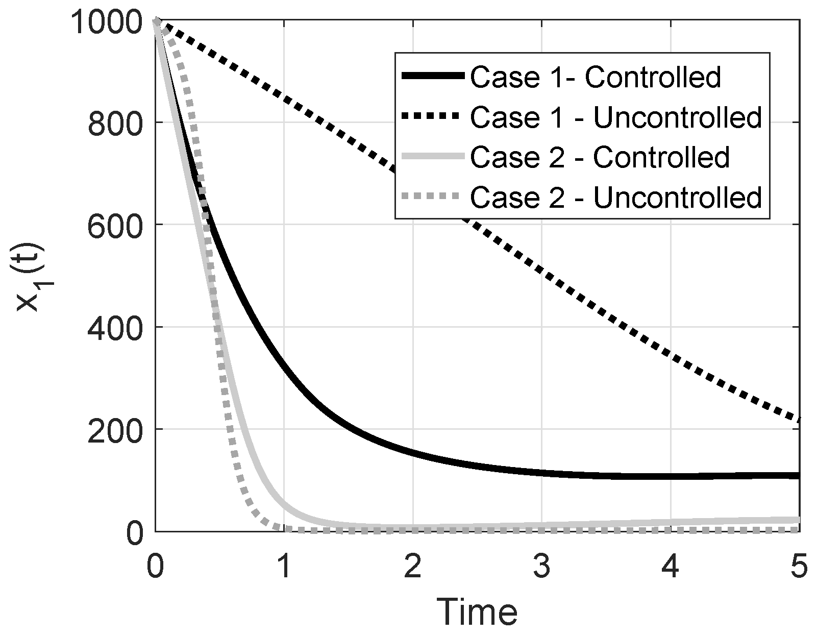
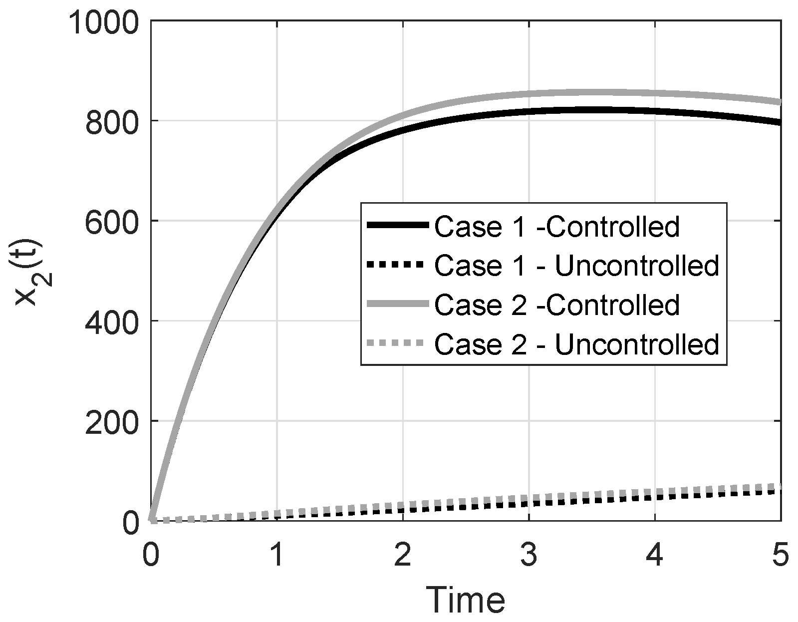
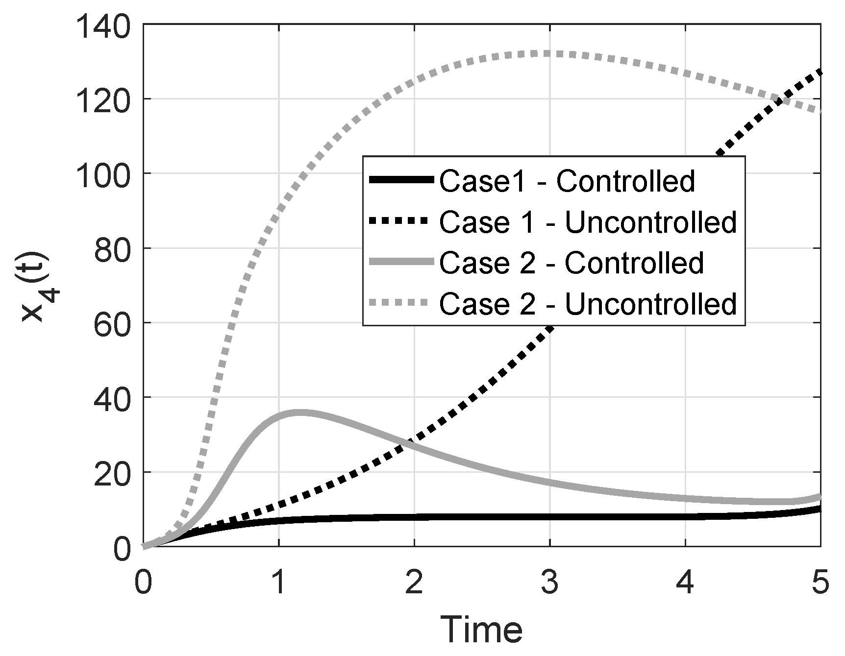
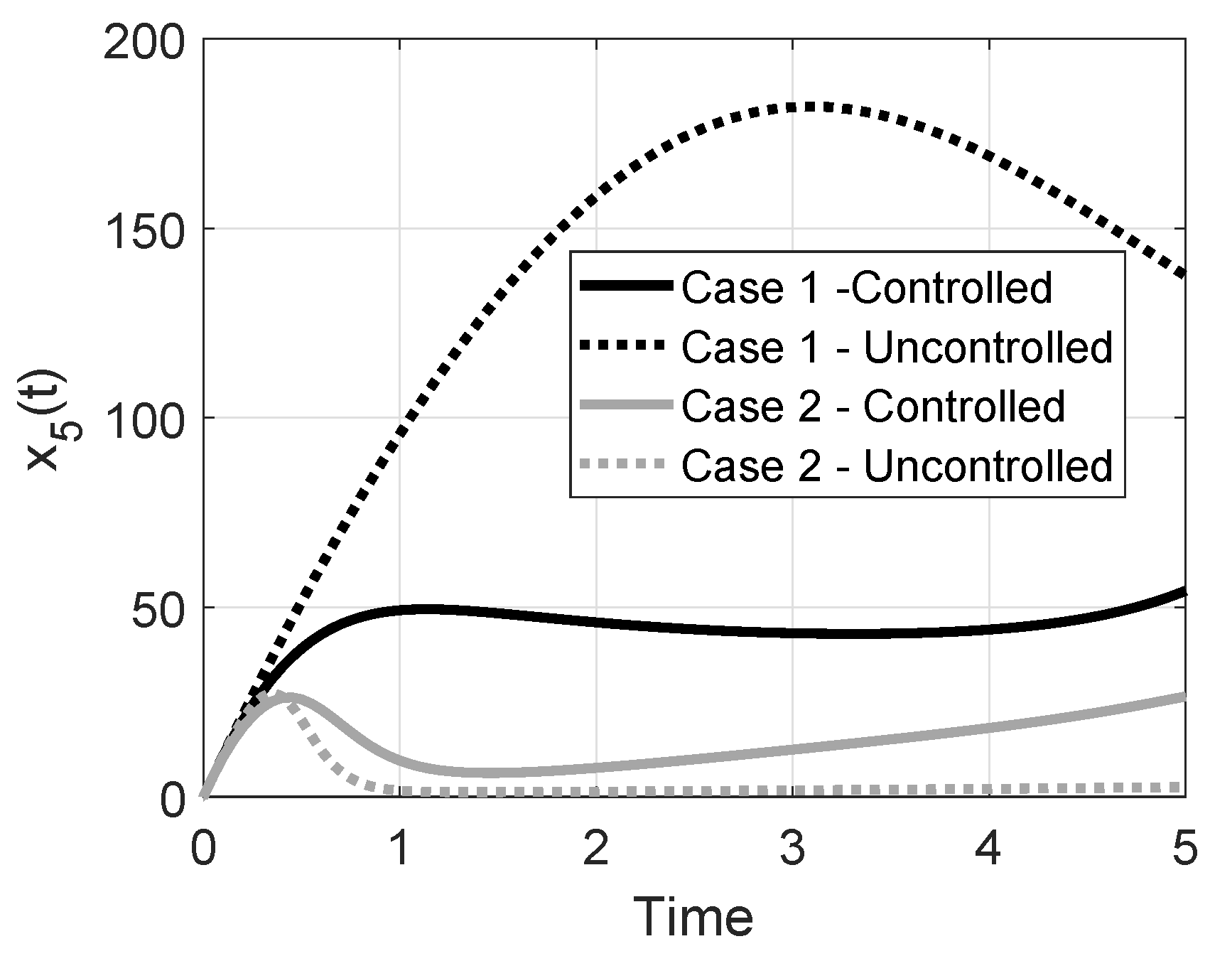
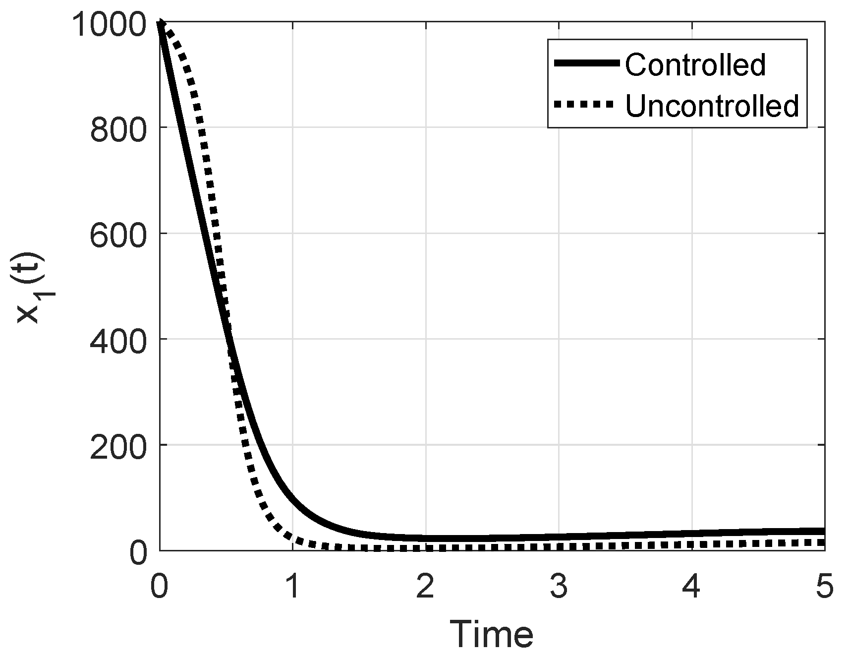
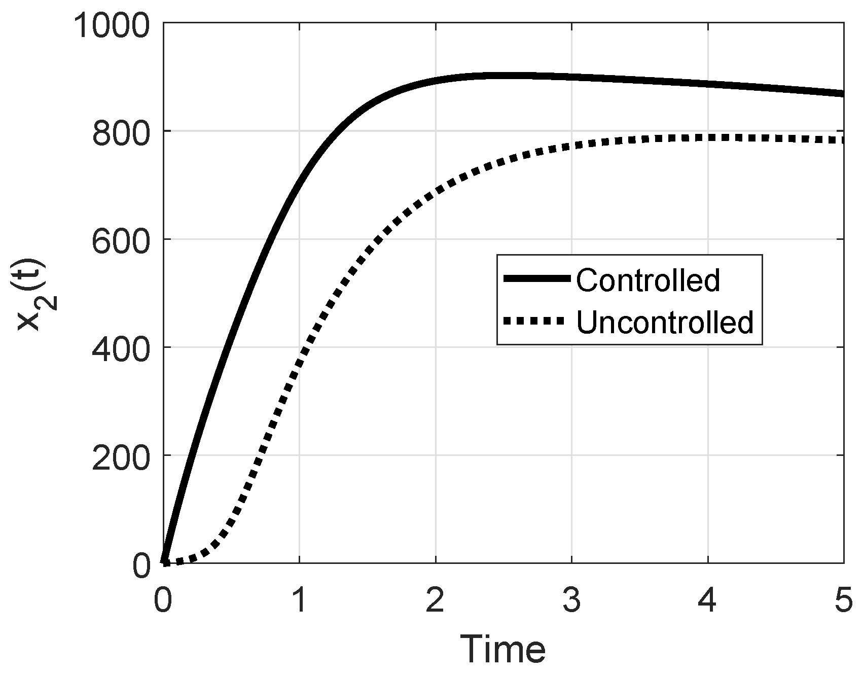
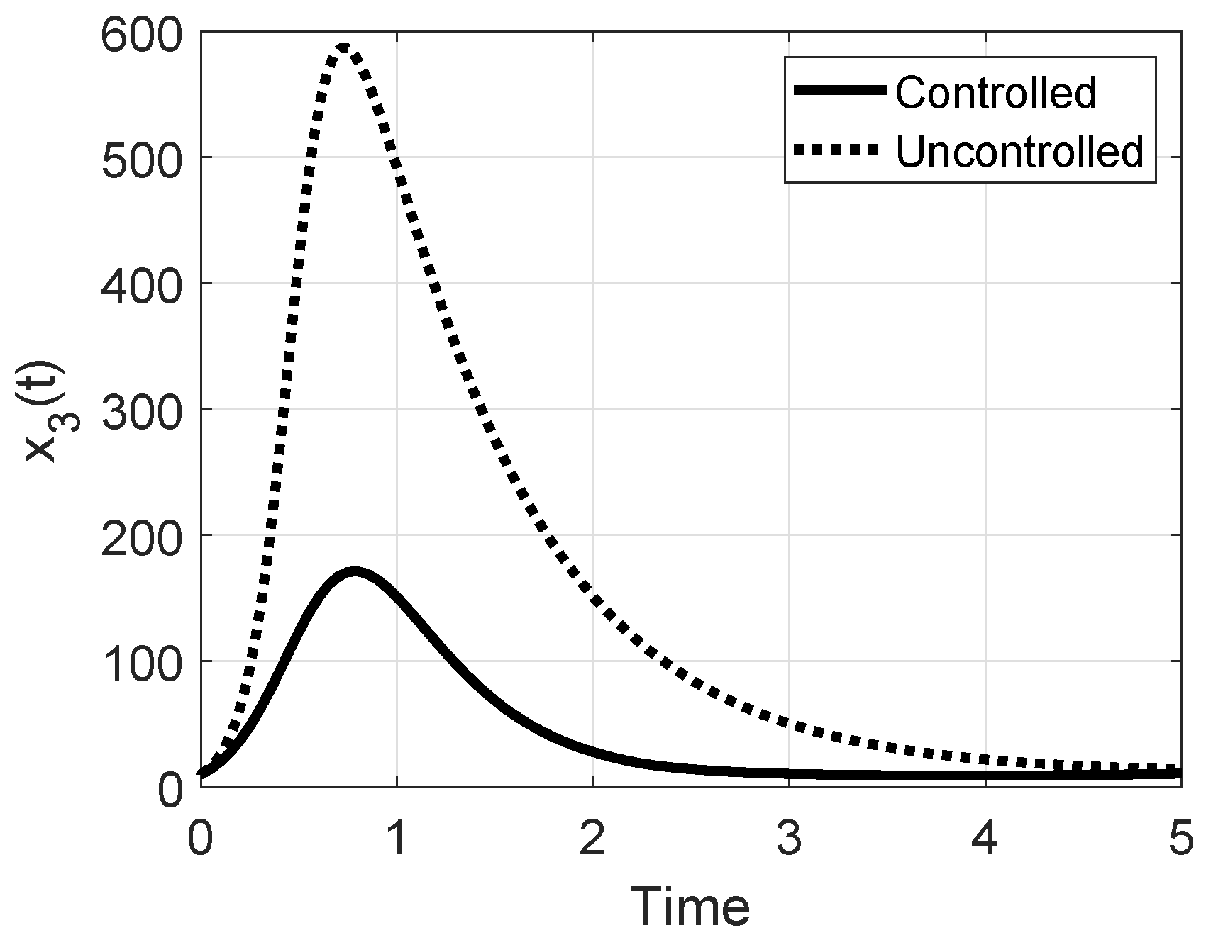
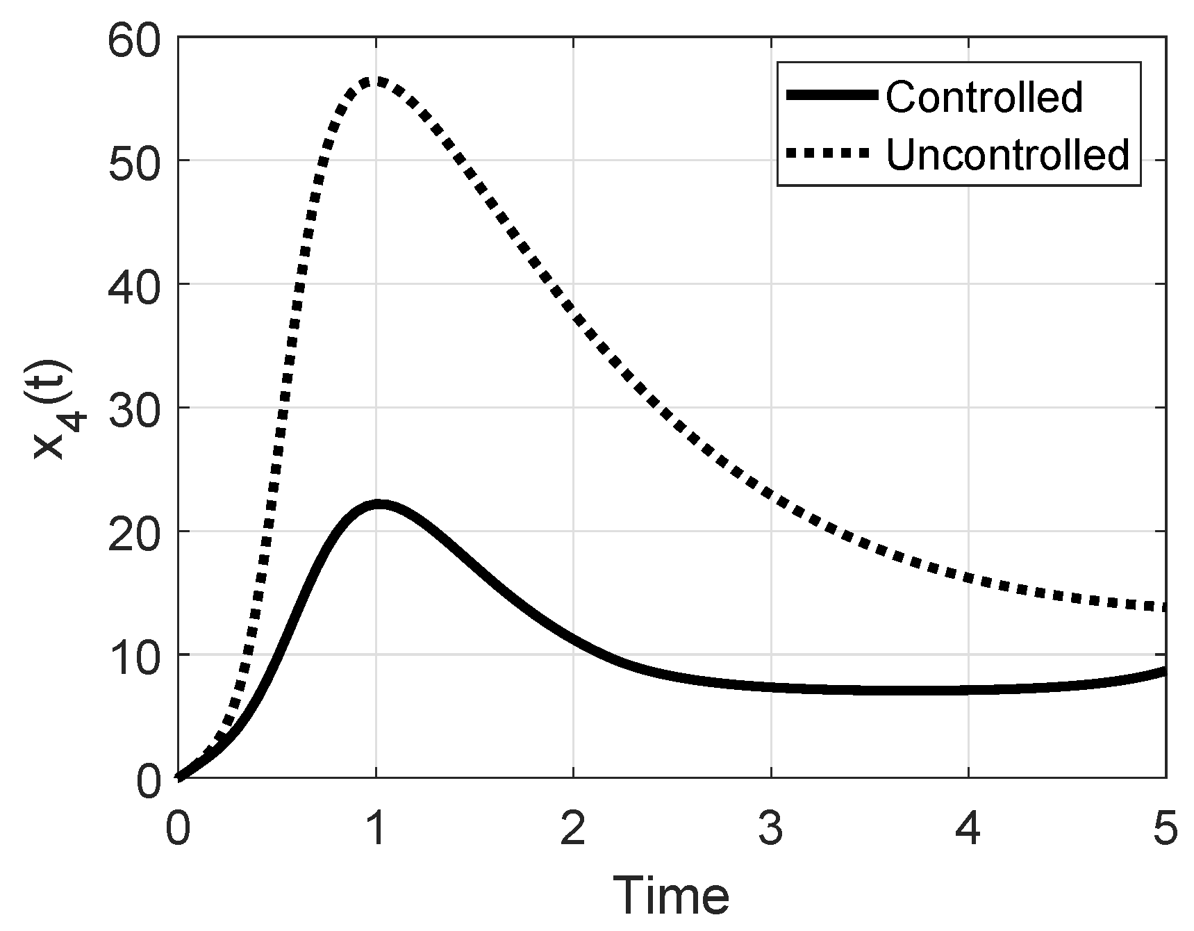
In Figure 5, Figure 6, Figure 7, Figure 8 and Figure 9 the evolutions of the states $x_i\left(t\right)$, $i=1,\dots ,5$ are shown along with the same quantities when no control is applied, comparing Case 1 and Case 2. The state evolutions corresponding to the immune subjects $x_2\left(t\right)$ do not vary significantly in the two situations, whereas the dangerousness of Case 2 is evident in the non-controlled case for the evolution of $x_3\left(t\right)$ and $x_4\left(t\right)$ patients, reaching higher values than in Case 1, Figure 7 and Figure 8. Nevertheless, the control actions can reduce the peaks significantly.

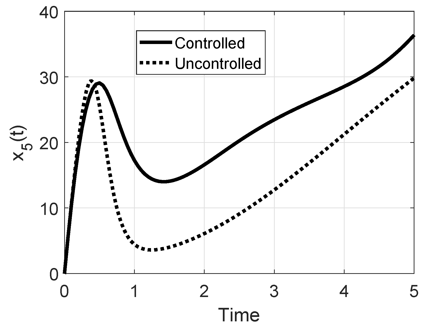
As for the evolution of the subjects $x_5\left(t\right)$, it can be noted that they increase more in the Case 1 than in Case 2; this is reasonable since in Case 1, the epidemic disease is not spreading and therefore the subjects will transit mainly in the $x_1$, $x_2$, and $x_5$ classes.

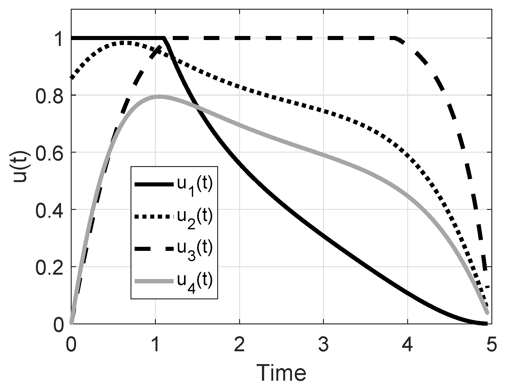
In Figure 10 the optimal controls $u_i\left(t\right)$, $i=1,\dots ,4$ are shown for Case 1. The epidemic spread is not a risky one, the value of $\beta$ being small; nevertheless, the control actions allow the decrease of the number of subjects $x_3\left(t\right)$, $x_4\left(t\right)$, $x_5\left(t\right)$, as well as of the $x_1\left(t\right)$ individuals, which also decreases without control, but less rapidly.

The control actions show a strong effort in vaccination up to about 1 year, while, as expected, the therapy action on the subjects in the most risky condition of the patients in the $x_4$ class must be applied for almost all the control periods. Please note that the control $u_4$ does not reach the maximum value allowed. This is an example of an efficient allocation strategy: it appears more convenient to vaccinate the subjects with maximum effort at the beginning of the control period and then, while $u_1$ decreases, the therapy must reach its maximum.

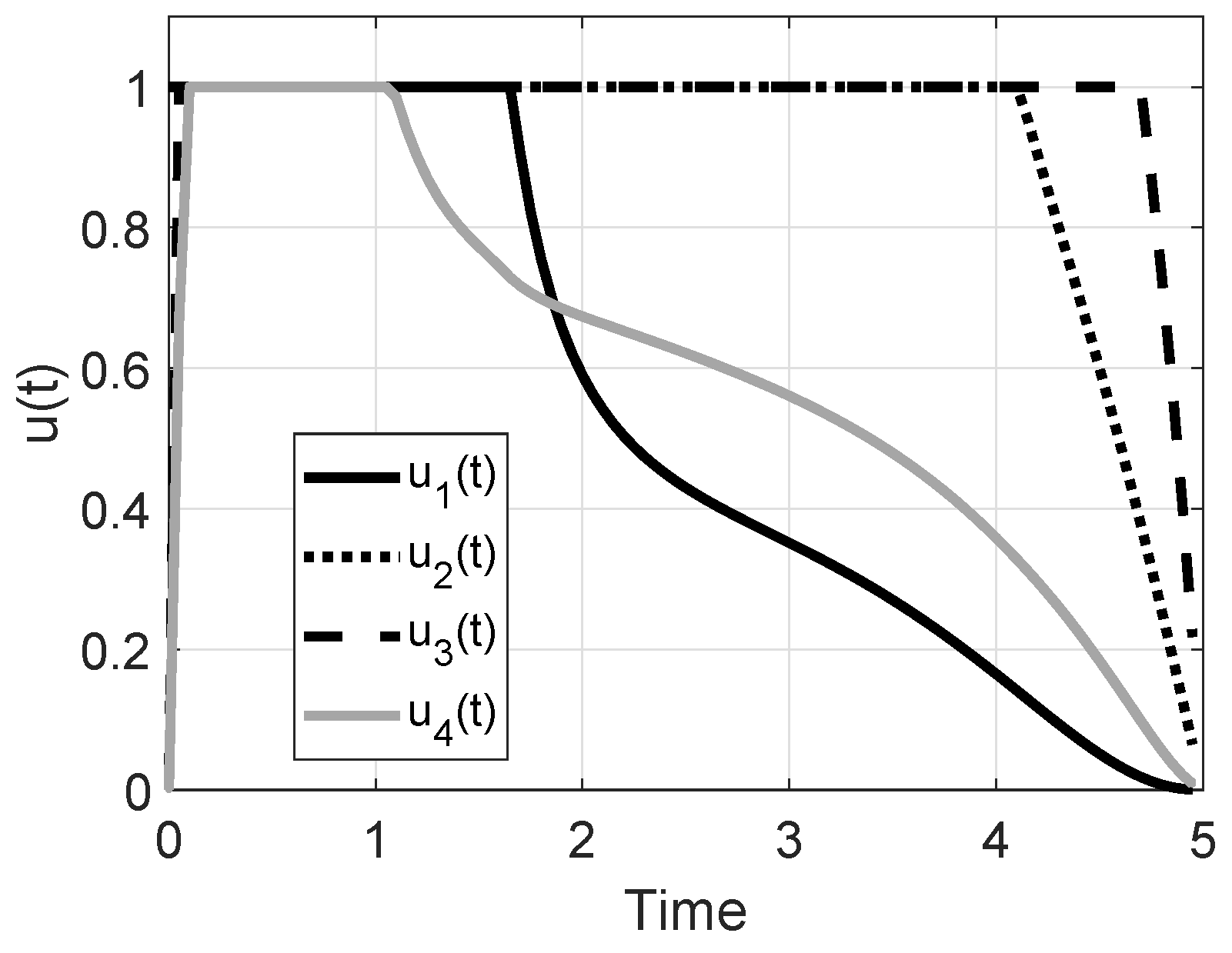
In Case 2 a stronger control action is required than in Case 1, Figure 11: maximum effort of the vaccination up to almost 2 years, the therapy on the $x_3$ subjects up to the fourth year and the therapy over the $x_4$ subjects for almost all the control period. The control over the $x_5$ subjects must be applied at its maximum value only for the first year, and then it decreases.

The effectiveness of the control procedure is evaluated also by considering the indicators V, $C_i$, $i=1,\dots ,4$ and E introduced; an efficient control would yield a strong decrease of dead patients (and therefore a negative V, as small as possible), a low control cost C, and also a low value of E.

In

Table 1. Comparison.

$\mathit{Case}$	V (%)	${\mathit{C}}_1$	${\mathit{C}}_2$	${\mathit{C}}_3$	${\mathit{C}}_4$	E
Case 1	−73.73	2.46	3.68	4.25	2.57	551.69
Case 2	−83.27	2.70	4.60	4.84	3.02	2067
Case 3	−83.40	2.10	4.96	4.95	4.65	2325
Case 4	−83.27	4.34	4.53	4.83	3.09	2276
Case 5	−70.65	2.24	3.29	3.91	2.12	868
Case 6	−95.18	4.03	5.06	5.67	3.03	762

the sensible decrease of the number of dead patients is shown, once the control is applied; the cost is obviously higher in Case 2, since the epidemic spread is more dangerous and thus requires a greater effort. As far as the E parameter, it increases sensibly in Case 2 with respect to Case 1 since, as said, it is costlier than the control, and there are a higher the number of dead patients. Leaving $\beta =0.01$ as in Case 2, if a stronger weight is assigned to the vaccination $u_1$ with respect to the other $r_i$, say $r_1=10$, $r_i=1$, $i=2,3,4$, the consequence is that the vaccination effort should be maximized more than the other controls aiming at the same goal; this condition is referred to as Case 3 in Table 1. Please note that to compensate for the smaller vaccination effort, the other controls must be increased. The symmetric situation is analyzed in Case 4, by assigning $r_1=1$, $r_i=10$, $i=2,3,4$; this means that the increase of the vaccination effort is allowed; the higher cost $C_1$, even if the global parameter E slightly decreases can be noted, since costs $u_i$, $i=2,3,4$ are lower.

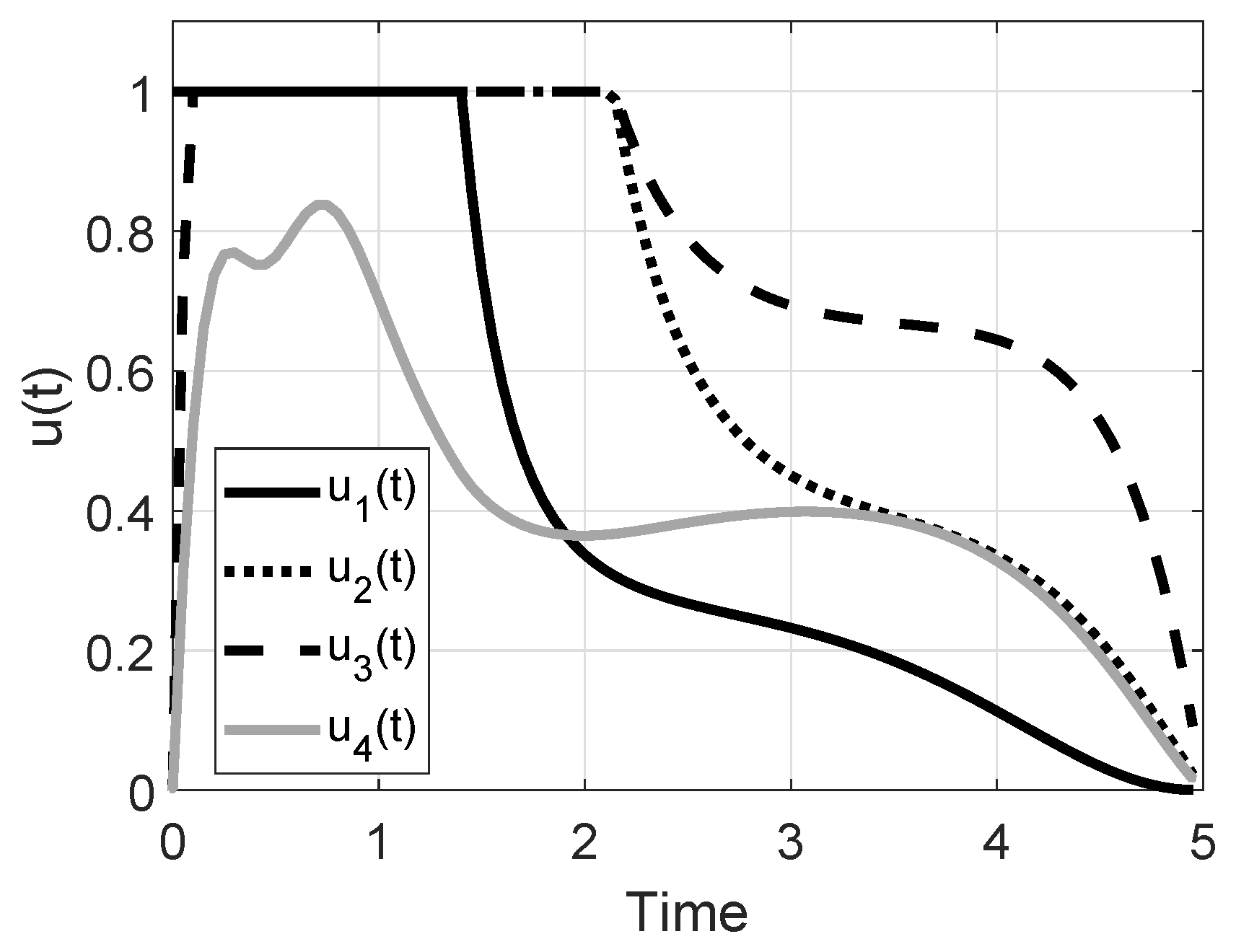
As already noted, the proposed model introduces some innovation with respect to the one presented in [19]; in particular, the possibility of spontaneous healing of $x_3$ and $x_4$ patients is allowed; in the considered Cases 1–4 they have been fixed equal to $0.01$, of the same order of magnitude of the parameters for the mortality. If they are increased sensibly, for example up to 1, a strong capability of the patients in the $x_3$ and $x_4$ classes to recover is assumed; this could be the realistic situation of a population in a good general healthy condition. In this case, as denoted in Case 5 and obtained with the other parameters as the ones in Case 2, the very low value of the E parameter can be noted, denoting a small number of dead people, as well as a decreased value of control costs. Moreover, all the cost efforts are decreased with respect to all the other cases, also compared to the Case 1. The results of Case 5 are shown in Figure 12, Figure 13, Figure 14, Figure 15, Figure 16 and Figure 17. It can be noted that the introduction of the optimal control strongly reduces the peaks of infections for the $x_3$ and $x_4$ patients with a lower value of all the costs with respect to the previously discussed cases. What is suggested in Case 5 is the maximum effort for the controls $u_i$, $i=1,2,3$ up to the first year for the vaccination and to the second year for the other two controls $u_2$ and $u_3$. The therapy $u_4$ does not reach the maximum effort allowed. This result must be compared with the corresponding one of Figure 11 where a stronger effort is required for all the control period. Case 5 highlights the obvious fact that if a population is in general good health conditions, usually related to economic and social wellness, it has stronger healing capability and it is less expensive to face an epidemic disease and its complications.

Finally, in the last row of Table 1, Case 6 is proposed, considering the same situation as Case 2 but with the control effort not bounded, as in [19]. Obviously, the possibility of using unbounded control allows r sensible reduction of the number of dead patients ($-95\%$) but with a stronger control effort; in particular, the cost of the control $u_1\left(t\right)$, the vaccination, is almost doubled, thus confirming the importance of a fast prevention action.

5. Conclusions

The epidemiological scenario considered in this paper regards a homogeneous population threatened by an epidemic disease; a possible complication, not risky by itself, could become fatal if in conjunction with the infectious disease. This represents a realistic scenario, such as in measles, or in HIV/AIDS, where an already weakened patient could be at risk of complications. Similar considerations may be applied to the elderly population invited to be vaccinated to avoid the flu, for example, and consequently also to avert other diseases that, together with the main epidemic, can be fatal. The problem is current in the globalized world as well as in society with elderly individuals. Some correlations among different diseases have been studied in the last ten years (such as between tuberculosis and diabetes) showing the importance of a suitable modeling in view of predicting possible epidemic scenarios. The optimal control theory confirms its effectiveness in an efficient resource allocation in trying to prevent (by vaccination) and to limit (by therapy) epidemic spread. The principal role of vaccination and, most of all, of a coordinated global control action able to strongly reduce (more than halve) the peak of the number of patients also in case of severe epidemic spread is confirmed.

Future work will be devoted to the identification of the model parameters referring to specific epidemic disease and complications, as well as to a geographic and social scenario.

References

- Di Giamberardino, P.; Iacoviello, D. LQ control design for the containment of the HIV/AIDS diffusion. Control Eng. Pract. 2018, 77, 162–173. [Google Scholar] [CrossRef]
- Di Giamberardino, P.; Iacoviello, D. Modeling the effects of prevention and early diagnosis on HIV/AIDS infection diffusion. IEEE Trans. Syst. Man Cybern. Syst. 2017, 99, 1–12. [Google Scholar] [CrossRef]
- Yan, X.; Zou, Y. Optimal and sub-optimal quarantine and isolation control in SARS epidemics. Math. Comput. Model. 2008, 47, 235–245. [Google Scholar] [CrossRef]
- Ledzewicz, U.; Schattler, E. On optimal singular controls for a general SIR-model with vaccination and treatment. Discret. Contin. Dyn. Syst. 2011, 2, 981–990. [Google Scholar]
- Behncke, H. Optimal control of deterministic epidemics. Opt. Control Appl. Methods 2000, 21, 269–285. [Google Scholar] [CrossRef]
- Joshi, H.R. Optimal control of an HIV immunology mode. Opt. Control Appl. Methods 2002, 23, 199–213. [Google Scholar] [CrossRef]
- Tsai, A.C.; Mendenhall, E.; Trostle, J.A.; Kawach, I. Co-occurring epidemics, syndemics and population health. Lancet 2017, 389, 978–982. [Google Scholar] [CrossRef]
- Iacoviello, D.; Stasio, N. Optimal control for SIRC epidemic outbreak. Comput. Methods Programs Biomed. 2013, 110, 333–342. [Google Scholar] [CrossRef] [PubMed]
- Xu, Y.; Ren, J. Propagation effect of a virus outbreak on a network with limited anti-virus ability. PLoS ONE 2016, 27, e0164415. [Google Scholar] [CrossRef] [PubMed]
- Zhu, Q.; Yang, X. Modeling and analysis of the spread of computer virus. Commun. Nonlinear Sci. Numer. Simul. 2012, 17, 5117–5124. [Google Scholar] [CrossRef]
- Ahmed, I.H.I.; Witbooi, P.J.; Patida, K. Modeling the dynamics of an epidemic under vaccination in two interacting populations. J. Appl. Math. 2012, 2012, 275902. [Google Scholar] [CrossRef]
- Rowthorn, R.E.; Laxminarayan, R.; Gilligan, C.A. Optimal control of epidemics in metapopulations. J. R. Sci. Interface 2009, 6, 1135–1144. [Google Scholar] [CrossRef] [PubMed] [Green Version]
- Dooley, K.E.; Chaisson, R.E. Tuberculosis and diabetes mellitus: convergence of two epidemics. Lancet Infect. Dis. 2010, 8, 4–15. [Google Scholar] [CrossRef]
- Newman, M.E.J.; Ferrario, C.R. Interacting epidemics and coinfection on contact networks. PLoS ONE 2009, 8, e71321. [Google Scholar] [CrossRef] [PubMed]
- Sutiono, A.B.; Suwa, H.; Ohta, T. Multi agent based simulation for typhoid fever with complications: An epidemic analysis. In Proceedings of the 51st Annual Meeting of the International Society for the Systems Sciences, Tokyo, Japan, 5–10 August 2007; pp. 4–15. [Google Scholar]
- Zhou, Y.; Yang, K.; Zhou, K.; Wang, C. Optimal treatment strategies for HIV with antibody response. J. Appl. Math. 2014, 27, 1–13. [Google Scholar] [CrossRef]
- Di Giamberardino, P.; Iacoviello, D. Optimal Control of SIR Epidemic Model with State Dependent Switching Cost Index. Biomed. Signal Process. Control 2017, 31, 377–380. [Google Scholar] [CrossRef]
- Iacoviello, D.; Liuzzi, G. Fixed/free final time SIR epidemic models with multiple controls. Int. J. Simul. Model. 2008, 7, 81–92. [Google Scholar] [CrossRef]
- Di Giamberardino, P.; Iacoviello, D. Modeling and control of an epidemic disease under possible complication. In Proceedings of the 22nd International Conference on System Theory, Control and Computing, Sinaia, Romania, 10–12 October 2018; pp. 87–92. [Google Scholar]
- Van Den Driessche, P.; Watmough, J. Reproduction numbers and sub-threshold endemic equilibria for compartmental models of disease transmission. Math. Biosci. 2002, 18, 29–48. [Google Scholar] [CrossRef]
- Van Den Driessche, P. Reproduction numbers of infectious disease models. Infect. Dis. Model. 2017, 2, 288–303. [Google Scholar] [CrossRef] [PubMed]
Figure 1.
Block diagram of the considered model.
Figure 2.
Evolutions of the five components of the point .
Figure 3.
Figure 4.
Eigenvalues of the Jacobian matrix evaluated for , , , , .
Figure 5.
Evolution of the number of subjects in Case 1 (black line) and Case 2 (grey line) with (continuous line) and without control (dotted line).
Figure 6.
Figure 7.
Figure 8.
Figure 9.
Figure 10.
Case 1: evolution of the optimal control actions.
Figure 11.
Case 2: evolution of the optimal control actions.
Figure 12.
Case 5: evolution of the number of with (continuous line) and without control (dotted line).
Figure 13.
Figure 14.
Figure 15.
Figure 16.
Figure 17.
Case 5: evolution of the optimal control actions.