
“Dividing and Conquering” and “Caching” in Molecular Modeling


1
School of Life Sciences, Jilin University, Changchun 130012, China
2
School of Artificial Intelligence, Jilin University, Changchun 130012, China
*
Author to whom correspondence should be addressed.
Int. J. Mol. Sci. 2021, 22(9), 5053; https://doi.org/10.3390/ijms22095053
Submission received: 3 March 2021
/
Revised: 26 April 2021
/
Accepted: 27 April 2021
/
Published: 10 May 2021
(This article belongs to the Special Issue Advances in Molecular Simulation)
Abstract
:Molecular modeling is widely utilized in subjects including but not limited to physics, chemistry, biology, materials science and engineering. Impressive progress has been made in development of theories, algorithms and software packages. To divide and conquer, and to cache intermediate results have been long standing principles in development of algorithms. Not surprisingly, most important methodological advancements in more than half century of molecular modeling are various implementations of these two fundamental principles. In the mainstream classical computational molecular science, tremendous efforts have been invested on two lines of algorithm development. The first is coarse graining, which is to represent multiple basic particles in higher resolution modeling as a single larger and softer particle in lower resolution counterpart, with resulting force fields of partial transferability at the expense of some information loss. The second is enhanced sampling, which realizes “dividing and conquering” and/or “caching” in configurational space with focus either on reaction coordinates and collective variables as in metadynamics and related algorithms, or on the transition matrix and state discretization as in Markov state models. For this line of algorithms, spatial resolution is maintained but results are not transferable. Deep learning has been utilized to realize more efficient and accurate ways of “dividing and conquering” and “caching” along these two lines of algorithmic research. We proposed and demonstrated the local free energy landscape approach, a new framework for classical computational molecular science. This framework is based on a third class of algorithm that facilitates molecular modeling through partially transferable in resolution “caching” of distributions for local clusters of molecular degrees of freedom. Differences, connections and potential interactions among these three algorithmic directions are discussed, with the hope to stimulate development of more elegant, efficient and reliable formulations and algorithms for “dividing and conquering” and “caching” in complex molecular systems.
1. Introduction
The impact of molecular modeling in scientific research is clearly embodied by the number of publications. Statistics from a Web of Science (www.webofknowledge.com (accessed on 15 February 2021)) search with various relevant key words is listed in Table 1. However, despite widespread applications of molecular modeling, we remain far from accurately predicting and designing molecular systems in general. Further methodological development is highly desired to tap its full potential. Historically, molecular modeling has been approached from a physical or application point of view, and numerous excellent reviews are available in this regard [1,2,3,4,5,6,7,8,9,10,11,12,13,14,15,16]. From an algorithmic perspective, “dividing and conquering” (DC) and “caching” intermediate results that need to be computed repetitively are two fundamental principles in development of many important algorithms (e.g., dynamic programming [17]). As a matter of fact, the major focus of modern statistical machine learning is to learn (“caching” relevant information) and then carry out inference on top of which [18]. In this review, we provide a brief discussion of important methodological development in molecular modeling as specific applications of these two principles. The content will be organized as follows. Part 2 describes fundamental challenges in molecular modeling; Part 3 summarizes application of these two fundamental algorithmic principles in two lines of methodological research, coarse graining (CG) [18,19,20,21,22,23,24,25,26,27] and enhanced sampling (ES) [28,29,30,31]; Part 4 covers how machine learning, particularly deep learning, facilitates DC and “caching” in CG and ES [29,30,32,33,34,35], Part 5 introduces local free energy landscape (LFEL) approach, a new framework for computational molecular science based on partially transferable in resolution “caching” of local sampling. The first implementation of this new framework in protein structural refinement based on generalized solvation free energy (GSFE) theory [36] is briefly discussed; and Part 6 discusses connections among these three lines of algorithmic development, their specific advantages and prospective explorations. Due to the large body of literature and limited space, we apologize to authors whose excellent works are not cited here.
2. Challenges in Molecular Modeling
2.1. Accurate Description of Molecular Interactions
Molecular interactions may be accurately described with high level molecular orbital theories (e.g., coupled cluster theory [37,38]) or sophisticated density functionals combined with large basis sets [39,40,41,42,43]. However, such quantum mechanically detailed computation is prohibitively expensive for any realistic complex molecular systems. Molecular interactions are traditionally represented by explicit functions and pairwise approximations as exemplified by typical physics based atomistic molecular mechanical (MM) force fields (FFs) [44,45,46,47]:
or knowledge based potential functions [48,49,50]: these simple functions, while being amenable to rapid computation and are physically sound grounded near local energy minima (e.g., harmonic behavior of bonding, bending near equilibrium bond lengths and bend angles), are potentially problematic for anharmonic interactions, which are very common in some molecular systems [51]. It is well understood that properly parameterized Lennard–Jones potentials are accurate only near the bottom of its potential well. Frustration are ubiquitous in biomolecular systems and are likely fundamental driving force for conformational fluctuations [52,53,54]. One may imagine that a molecular system with all its comprising particles at their respective “happy” energy minima positions would likely be a stable “dead” molecule, which may be a good structural support but is likely not able to provide dynamic functional behavior.
Pairwise approximations are usually adopted for its computational convenience, both in terms of dramatically reduced computational cost and tremendously smaller (when compared with possible many body potentials) number of necessary parameters to be fit in FF parameterization. It is widely acknowledged that construction of traditional FF (e.g., Equation (1)) is a laborious process. Development of polarizable [9,55,56] and more complex FF with larger parameter set [57] alleviates some shortcomings of earlier counterpart. Expansion based treatments were incorporated to address anharmonicity [58]. However, to tackle limitation of explicit simple functional form and pairwise approximation for better description of molecular interactions remains challenge to be met for molecular modeling community. Additionally, even atomistic simulations are prohibitively expensive for large biomolecular complexes at long time scales (e.g., milliseconds and beyond) [59,60,61].
2.2. Inherent Low Efficiency in Sampling of Configurational Space
Complexity of molecular systems is rooted in their molecular interactions, which engender complex and non-linear correlations among molecular degrees of freedom (DOFs). Consequently, effective number of DOFs are greatly reduced. Therefore, complex molecular systems are confined to manifolds [62] of much lower dimensionality with near zero measure in corresponding nominal high dimensional space (NHDS). Consequently, sufficient brute force random sampling in NHDS of interested molecular systems is hopeless.
In stochastic trajectory generation by Monte Carlo (MC) simulations or candidate structural model proposal in protein structure prediction and refinement (or other similar scenarios), new configuration proposal is carried out in NHDS. A lot of effort is inevitably wasted due to sampling outside the actual manifold occupied by the target molecular system. Such wasting may be avoided if we understood all correlations. However, understanding all correlations implicates accurate description of global free energy landscape (FEL) and there is no need to investigate it further. Due to preference of lower energy configurations by typical importance sampling strategies (e.g., Metropolis MC), stochastic trajectories tend to be trapped in local minima of FEL. This is especially true for complex molecular (e.g., biomolecular) systems which have hierarchical rugged FEL with many local minima [63,64]. In trajectory generation by molecular dynamics (MD) simulations, configurational space is explored by laws of classical mechanics and no wasting due to random moves exists. However, molecular systems may well drift away from their true manifolds due to insufficient accuracy of FF, resulting incorrect and wasted sampling. Similar to stochastic trajectory generation, it takes long simulations to map FEL since molecular system tend to staying at any local minimum, achieve equilibrium among many local minima is just as challenging as in the case of stochastic counterpart.
3. DC and “Caching” in Traditional Molecular Modeling
To cope with fundamental difficulties in molecular modeling, two distinct lines of methodological development (CG and ES) based on DC and “caching” strategies have been conducted and tremendous progress has been made in understanding of molecular systems. As summarized below:
3.1. Coarse Graining, a Partially Transferable “Caching” Strategy
Atomistic FF parameterization is the most well established coarse graining based on time scale separation between each nuclei and its surrounding electrons. Theoretically, MMFFs are potential of mean force (PMF) obtained by averaging over many electronic DOFs for given atomic configurations. In practice, due to the fact that ab initio calculations are expensive and may have significant error when level of theory (and/or basis set) is not sufficient, reference data usually include results from both quantum mechanical (QM) calculations and well-established experimental data [65,66,67]. The DC strategy is utilized by selecting atomic clusters of various size to facilitate generation of QM reference data. The essential information learned from reference data is then permanently and approximately “cached” in FF parameters through the parameterization process. Time scale separation ensures that elimination of electronic DOFs is straight forward but comes with the price of incapability in describing chemical reactions. To harvest benefits of both quantum and atomistic simulations, a well-established DC strategy is to treat a small region involved in interested chemical reaction at QM detail and its surrounding with MMFF [68,69,70,71,72,73]. This series of pioneering work was awarded Nobel prize in 2013, and QM-MM treatment continues to be the mainstream methodology for computational description of chemical reactions [74,75].
The united atom model (UAM) is the next step in coarse graining [76], where hydrogen atoms are merged into bonded heavy atoms. This is quite intuitive since hydrogens have much smaller mass on the one hand, and are difficult to see by experimental detection techniques utilizing electron diffraction (e.g., X-ray crystallography) on the other hand. For both polymeric and biomolecular systems, UAM remains to be expensive for many interested spatial and temporal scales. Therefore, further coarse graining in various forms have been constructed. As a matter of fact, CG is usually used to denote modeling with particles that representing multiple atoms in contrast to atomistic simulations, and the same convention will be adopted in the remaining part of this review unless stated otherwise. Both “Top-down” (that based on reproducing experimental data) and “bottom-up” ( that based on reproducing certain properties of atomistic simulations) approaches are utilized [21,77]. For polymeric materials, beads are either utilized to represent monomers or defined on consideration of persistent length [78], and dissipative particle dynamics (DPD) were proposed to deal with complexities arise from much larger particles [79]. For biomolecular systems, a wide variety of coarse grained models have been developed [20,21,23,24,80,81]. Another important subject of CG methodology development is materials science [82,83]. Earlier definition of CG particles are rather ad hoc [20]. More formulations with improved statistical mechanical rigor appeared later on [22], with radial distribution function based inversion [78,84,85,86], entropy divergence [19] and force matching algorithm [87,88,89] being outstanding examples of systematic development. Present CG is essentially to realize the following mapping as disclosed by Equation (4) in ref. [22]:
with and being coordinates in higher resolution and CG coordinates, being the map operator from to , V and being relevant potential of mean force in higher resolution and CG representation respectively. Due to lack of time scale separation (see Figure 1) for essentially all CG mapping, strict realization of this equation/mapping with exact transferability is not rigorously possible. A naive treatment of CG particles as basic units (with no internal degrees of freedom) would result in wrong thermodynamics [22]. Due to corresponding significant loss of information, it is not possible to develop a definition of CG and corresponding FF parameterization for comprehensive reproduction of atomistic description of corresponding molecular systems. Different coarse graining have distinct advantages and disadvantages, so choosing proper CG strategy is highly dependent upon specific goal in mind. CG particles are usually isotropic larger and softer particles with pairwise interactions, or simple convex anisotropic object (e.g., soft spheroids) that may be treated analytically [24,90,91,92]. Such simplifications provide both convenience of computation and certain deficiency for capturing physics of target molecular systems. CG may be carried out iteratively to address increasingly larger spatial scales by “caching” lower resolution CG distributions with ultra CG (UCG) FF [22,93,94,95,96,97]. Pairwise approximation remains to be limitation of interaction description for traditional CG FF, which may use either explicit simple function form or tables. When compared with atomistic FF, pairwise approximation deteriorate further due to lack of time scale separation (Figure 1).
Another simple and powerful type of CG model for biomolecular systems is Gō model [98,99] and elastic network models (ENM) [100,101,102] or gaussian network models (GNM) [103,104] with native structure being defined as the equilibrium state, and with quadratic/harmonic interactions between all residues within given cutoff. Only a few parameters (e.g., cutoff distance, spring constant) are needed. Such models “caching” the experimental structures and are proved to be useful in understanding major conformational transitions and slow dynamics of many biomolecular systems [105,106].
3.2. Enhanced Sampling, a Nontransferable in Resolution DC and “Caching” Strategy
Umbrella sampling (US) [107] is probably the first combination of DC and “caching” strategy for better sampling of molecular system along a given reaction coordinate (RC) (or order parameter) s. DC strategy is first applied by dividing s into windows, information for each window is then partially “cached” by corresponding bias potentials and local statistics. Later on, adaptive US (AUS) [108,109] and weighted histogram analysis method (WHAM) [110] were developed to improve both efficiency and accuracy. MBAR [111,112] was developed to achieve error bound analysis which was not available in WHAM. Further development including adaptive bias force (ABF) [113,114,115] and metadynamics [116,117,118]. Details of these methodologies were well explained by excellent reviews [119,120,121,122]. The common trick to all of these algorithms (and their variants) is to “cache” visited configurational space with bias potentials/force and local statistics, thus reduce time spent in local minima and dramatically accelerate sampling of interested rare events. Denote CV as ( being physical coordinates of atoms/particles in the target molecular system), equilibrium distribution and free energy on the CV may be expressed as [30]:
with being the sampled distribution in simulations with corresponding bias potential for “caching” of visited configurational space.
The starting point of these “caching” algorithms is specification of reaction coordinates (RC) or collective variables (CVs), which is a very challenging task for complex molecular systems in many cases. Traditionally, principle component analysis (PCA) [123] is the most widely utilized and a robust way for disclosing DOFs associated with the largest variations. To deal with ubiquitous nonlinear correlations, kernels are often used albeit with the difficulty of choosing proper kernels [124]. Additional methodologies, include multidimensional scaling (MDS) [125], isomap [126], locally linear embedding (LLE) [127], diffusion map [128,129] and sketch map [130] have been developed to map out manifold for high dimensional data. However, each has it own limitations. For example, LLE [127] is sensitive to noise and therefore has difficulty with molecular simulation trajectories which are quite noisy; Isomap [126] requires relatively homogeneously sampled manifold to be accurate. Both LLE and Isomap do not provide explicit mapping between molecular coordinates and CVs; diffusion and sketch maps are likely to be more suitable to analyze molecular simulation trajectories. Nonetheless, their successful application for large and complex molecular systems remains to be tested. All of above non-linear mapping algorithm are mainly suitable for manifold on a single scale, and capturing manifold on multiple scales simultaneously in molecular simulations has not been reported yet. When we are interested in finding paths for transitions among known metastable states, transition path sampling (TPS) [131,132,133] methodology maybe utilized to establish CV.
Apparently, RC and/or CV based ES is a different path for facilitate simulation of complex molecular systems on longer time scales from coarse graining. One apparent plus side is that these algorithms are “in resolution” as no systematic discarding of molecular DOFs occur. With specification of RC and/or CVs, computational resource is presumably directed toward the most interesting dynamics of the target molecular system, and RC and/or CV maybe repetitively refined to obtain mechanistic understanding of interested molecular processes. However, the down side is that “cached” information on local configurational space is not transferable to other similar molecular systems. While rigorous transferability may not be easily established for any CG FF, practical utility of CG FF for molecular systems with similar composition and thermodynamic conditions have been quite common and useful [24]. Therefore, CG FF may be deemed as partially transferable.
An important recent development of DC strategy for enhanced sampling is Markov state models (MSM) [134,135,136,137], one great advantage of which is that no RC or CV is needed. Instead, it extracts long-time dynamics from independent short trajectories distributed in configurational space. Many important biomolecular functional processes have been characterized with this great technique [138,139,140]. The most fundamental assumption is that all states for a target molecular system form an ergodic Markov chain:
with and being a vector of probabilities for all states at time t and respectively. is the transition matrix with its element being probability of the molecular system being found in state j after an implied lag time () from the previous state i. Apparently as t goes to infinity for an equilibrium molecular system, a stationary distribution will arise as defined below:
The advantage of not needing RC/CV does not come for free but with accompanying difficulties. Firstly, one has to distribute start points of trajectories to statistically important and different part of configurational space, then select proper (usually hierarchical, with each level of hierarchy corresponds to a specific lag time) partition of configurational space into discrete states. This is the key step of DC strategy in MSM. No formal rule is available and experience is important. In many cases some try and error is necessary. Secondly, within each discrete state at a given level of hierarchy, equilibration is assumed to be achieved instantly and this assumption causes systematic discretization error, which fortunately may be controlled with proper partition and sufficiently long lag time [141]. Apparently, metastable states obtained from MSM analysis is molecular system specific and thus not transferable.
Another important class of enhanced sampling is to facilitate sampling with non-Boltzmann distributions and restore property at targeted thermodynamic condition through proper reweight [142]. Most outstanding examples are Tsallis statistics [143,144], parallel tempering [145,146], replica exchange molecular dynamics [147,148], Landau-Wang algorithm [149] and integrated tempering sampling (ITS) [150,151,152]. These algorithms are not direct applications of DC and “caching” strategies and are not discussed further here.
4. Machine Learning Improves “Caching”
4.1. Toward Ab Initio Accuracy of Molecular Simulation Potentials
Fixed functional form and pairwise approximation of non-bonded interactions are two major factors limiting the accuracy of molecular interaction description in both atomistic and some CG FF. Neural network (NN) has capability of approximating arbitrary functions and therefore has potential to address these two issues. Not surprisingly, significant progress has been made in this regard as summarized by recent excellent reviews [27,153,154,155,156,157]. Cutoff and attention to local interactions remains the DC strategy for development of machine learning potentials. The major improvement over traditional FF is better “caching” that overcomes pairwise approximation and fixed functional form limitations. NN FF naturally tackle both issues as explicit functions are not necessary since NNs are universal approximators. The significance of many-body potentials [158] and extent of pairwise contributions were analyzed [159,160]. It is important to note that despite the fact that pairwise interactions account for the majority of energy contributions, high ordered interactions are likely to be significant in shaping differences of subtly distinct molecular systems. There are also efforts to search for different and proper simple functional forms, which are expected to be more accurate than present functional forms in traditional FF on the one hand, and alleviate overfitting/generalization difficulty and reduce computational cost of complex NN FF on the other hand [161,162], especially when training dataset is small. While most machine learning FF are trained by energy data [153,157], gradient-domain machine learning (GDML) approach [163] directly learns from forces and realizes great savings of data generation.
Just as in the case of traditional FF, transferability and accuracy is always a tradeoff. More transferability implicates less attention is paid to “cache” detailed differences among different molecular systems, hence less accuracy. Exploration in this regard, however, remains not as much as necessary [164,165,166]. Unlike manual fitting of traditional FF, systematic investigation of tradeoff strategies is potentially feasible for machine learning fitting [167], and yet to be done for many interesting molecular systems. With expediency of NN training, development of a NN FF hierarchy with increasing transferability/accuracy and decreasing accuracy/transferability is likely to become a pleasing reality in the near future. Rapid further development of machine learning potentials, particularly NN potentials, are expected. However, significant challenges for NN potentials remain on better generalization capability, description/treatment of long range interactions [168,169], wide range of transferability, [170] faster computation [171] and proper characterization of their error bounds. Should further significant progress be made on these issues, it is promising we may have routine molecular simulations with both classical efficiency and ab initio accuracy in the near future.
4.2. Machine Learning and Coarse Graining
As in the case of constructing atomic level potentials, machine learning has been applied to address two outstanding pending issues in coarse graining, which are definition of CG sites/particles and parameterization of corresponding interactions between/among these sites/particles. Traditional CG FF, suffers from both pairwise approximation and, for some, accuracy ceiling of simple fixed functional forms which are easy to fit. By using more complex (but fixed functional form) potentials with a machine learning fitting process, Chan et al. [172] developed ML-BOP CG water model with great success. Deep neural network (DNN) was utilized to facilitate parameterization of CG potentials when given radial distribution functions (RDF) from atomistic simulations [173]. CGnet demonstrated great success with simple model systems (alanine dipeptide) [174]. DeePCG model was developed to overcome pair approximation and fixed functional form and demonstrated with water [175]. Using oxygen site to represent water is rather intuitive. However, for more complex biomolecules such as proteins, possibility for selection of CG site explodes. To improve over intuitive or manual try and error definition of CG sites, a number of studies have been carried out [176,177,178,179] to provide better and faster options for choosing CG sites. However, no consensus strategy is available up to date and more investigations are desired. The fundamental difficulty is that there is no sufficient time scale separation between explicit CG DOFs and discarded implicit DOFs, regardless of specific selection scheme being utilized. Intuitively, one would expect CG FF parameters to be dependent upon definition of CG sites/particles. In this regard, auto-encoders were utilized to construct a generative framework that accomplishes CG representation and parameterization in a unified way [33]. The spirit of generative adversarial networks was utilized to facilitate CG construction and parameterization, particularly with virtual site representation [180]. It was found that description of off-target property by CG exhibit strong correlation with CG resolution, to which on-target property being much less sensitive [181]. Such observation suggests that adjust CG for specific target properties might be a better strategy than searching for a single best CG representation. Despite potentially more severe impact of pairwise approximation for CG FF than in atomistic FF, quantitative analysis in this regard remain to be done to the best of our knowledge.
4.3. Machine Learning in Searching for RC/CVs and Construction of MSM
To overcome difficulties of earlier nonlinear CV construction algorithms [126,127,128,130] and to reduce reliance on human experience, auto-encoders, which is well-established for trainable (non-linear) dimensionality reduction, are utilized in a few studies [182,183,184,185]. Chen and Ferguson [183] first utilized autoencoders to learn nonlinear CVs that are explicit and differentiable functions of molecular coordinates, thus enabling direct utility in molecular simulations for more effective exploration of configurational space. Further improvement [182] was achieved through circular network nodes and hierarchical network architectures to rank-order CVs. Wehmeyer and Noé [184] developed time-lagged auto-encoder to search for low dimensional embeddings that capture slow dynamics. Ribeiro et al. [185] proposed the reweighted autoencoded variational Bayes to iteratively refine RC and demonstrated in computation of the binding free energy profile for a hydrophobic ligand-substrate system. Building a MSM for any specific molecular system requires tremendous experience and many steps in process are error prone. To overcome these pitfalls, VAMPnet that based on variational approach for Markov process was developed to realize the complete mapping steps from molecular trajectories to Markov states [186]. As physical understanding of interested molecular systems is essential and the ultimate goal, application of these methods as black boxes are not encouraged.
5. The Local Free Energy Landscape Approach
Both CG and ES methodologies facilitate molecular simulation by effectively reducing local sampling. In CG, it is realized through “caching” (integration) of distributions for faster/discarded DOFs with proper CG FF, and thus has the inevitable cost of losing resolution (information), accompanied by the desired attribute of (partial) transferability to various extent. ES reduces lingering time of molecular systems in local minima through “caching” visited local configurational space, which is usually defined by relevant DC strategies, with biasing potentials. When compared with CG, there is no resolution loss. However, “cached” manifold of configurational space is molecular process specific and thus not transferable at all. In molecular modeling community, these two lines of methodologies are developed quite independently. Nevertheless, one might want to ask why not have both advantages in one method, that is to reduce repetitive local sampling without loss of resolution and with “cached” results being partially transferable. The local free energy landscape (LFEL) approach [187] is proposed with this intention in mind. Historically, parameterization of FF by coarse graining has been the only viable framework due to two fundamental constraints. Firstly, in earlier days of molecular modeling, typical computers have memory space of megabytes or less, render it impossible to accommodate millions or more parameters needed to fit complex LFEL; secondly, while both neural network and autodifferentiation were invented decades ago, the computational molecular science community did not master these techniques for fitting large number of parameters efficiently until recently. With these two constraints removed, possibility for alternative path arise to break monopoly of classical molecular modeling by FF parameterization via coarse graining. Specifically, one may carry out direct fitting of LFEL and all important information on local distributions of molecular DOFs obtained from expensive local sampling may be “cached”. This is in strong contrast to coarse graining based parameterization, in which local distributions are substituted by averaging in relevant lower dimensional space projection (e.g., pairwise distances among CG sites). However, it is essential to assemble LFEL and construct FEL of the interested molecular system, and this is the core of the LFEL approach. For a molecular system with N DOFs, this LFEL approach may be expressed as:
an N-DOF molecular system is reorganized into M overlapping regions (Equation (9)), each region has some number of DOFs (Equation (10)). The key step of LFEL approach is expressed in Equation (11), in which the first product term (addressed as “local term(s)” hereafter) treat M regions as if they were independent, and all correlations among different regions are incorporated by the fraction term, which is termed global correlation fraction (GCF) and is extremely difficult, if ever possible, to be calculated directly. However, GCF is a unnormalized probability distribution, when all molecular DOFs in local terms are (approximately) sampled according to GCF, then we do not need GCF explicitly anymore (Equations (12) and (13)). GCF represents two types of global correlations. The first type is mediated correlations among different regions by the fact that they overlap, and relevant molecular DOFs in such overlapping space shared by different regions should have exact same state for all concerning regions. The second type is direct global correlations among molecular DOFs in different regions caused by genuine long-range interactions (e.g., electrostatic interactions). Satisfying the first type with sampling is trivial, and ensuring all overlapping regions share the exact same state is sufficient (Equations (12) and (13)). The second type of global correlations need more involved treatment. These equations are apparently of general utility for any multiple-variable (high-dimensional) problem. In the specific case of a complex molecular system, using one set of coordinates realizes the mediated contribution of GCF. The approximation in Equation (12) is made by ignoring the second type of global correlations. Free energy minimization of a molecular system in thermodynamic equilibrium may be treated as maximization of joint probability (Equation (13)). For molecular systems (or biological systems) off equilibrium, the joint distribution remains our focus despite free energy is not well defined anymore. A schematic representation of the LFEL approach in contrast to FF framework is shown in (Figure 2). While we only demonstrated GSFE implementation of LFEL at residue level for protein structural refinement. LFEL approach may be utilized to “cache” local distributions at any spatial scales. Just as there are many methodological developments in the mainstream FF framework, there are certainly many possible ways to develop algorithms in the LFEL approach. We explored a first step toward this direction through a neural network implementation of the generalized solvation free energy (GSFE) theory [36]. In GSFE theory, each comprising unit in a complex molecular system is solvated by its neighboring units. Therefore, each unit is both a solute itself and a comprising solvent unit of its solvent units. Let denote a region i defined by a solute and its solvent , a molecular system of N units has N overlapping regions. Each local term may be further expanded:
Both terms may be learned from either experimental or computational datasets, as long as they are sufficiently representative and reliable. The first term in Equation (14) is the likelihood term when is the given, it quantifies the extent of match between the solute and its solvent . The second term is the local prior term, it quantifies the stability of the solvent environment . Computation of the prior term is more difficult than the likelihood term, but certainly learnable when sufficient data is available. A local maximum likelihood approximation of GSFE (LMLA-GSFE) is to simply ignore local prior terms.
A particular implementation of the LMLA-GSFE for protein structure refinement with residues defined as comprising unit was conducted [187]. In this scheme, GSFE is integrated with autodifferentiation and coordinate transformation to construct a computational graph for free energy optimization. With fully trainable LFEL derived from backbone and atom coordinates of selected experimental protein structures, we achieved superb efficiency and competitive accuracy when compared with state of the art atomistic protein refinement refinement methodologies. With our newly developed pipeline, refinement of typical protein structure decoys (within 300 amino acids) takes a few seconds on a single CPU core, in contrast to a few hours by typical efficient sampling/minimization based algorithms (e.g., FastRelax [188]) and thousands of hours for MD based refinement [189]. In the latest CASP14 refinement contest (predictioncenter.org/casp14/index.cgi (accessed on 15 February 2021)), our method ranked the the first for the 13 targets with start GDT-TS score larger than 60. We expect incorporation of complete heavy atom information and local prior terms to further improve this method in the future. GSFE theory in particular and the LFEL approach in general, are certainly extendable to modeling of other soft matter molecular systems.
6. More on Connections among CG, ES and LFEL Approach
All of these algorithms have a common goal of accelerating computation of a joint distribution for a given molecular system at some target resolution, albeit from distinct perspectives. The fundamental underpinning is the fact that molecular correlations among its various DOFs limit a molecular system to a manifold of significantly lower dimension. Both ES and CG in the FF framework and the LFEL approach are distinct strategies to “cache” manifolds from either configurational space (Figure 3) or physical space perspective (Figure 4). Commonality and differences of these strategies are summarized in Table 2 and discussed below.
Both MSM and RC/CV based ES are designed to first describe local parts of the approximate manifold in the configurational space formed by all molecular DOFs of the target molecular system. Information for such local configurational space is partially “cached” either as bias potentials or transition counts, which are further processed to map FEL and dynamics of interested molecular processes. Computational process (or educated guess) for establishment of RC/CVs is essentially “caching” results from sampling/guessing local parts of the configurational as approximate relevant manifold (Figure 3B). Subsequent sampling along RC/CV is hoped to disclose our interested molecular processes (e.g., biomolecular conformational transitions, substrate binding/release in catalysis). Involved molecular DOFs for RC/CVs are not necessarily spatially adjacent on the one hand, and may be different for different molecular processes of the same molecular system. Apparently, RC/CVs are molecular process specific and not transferable, even among different molecular process of the same molecular system. Nonetheless, the methodology for searching CVs may be applied to many different molecular processes/systems.
In contrast, both CG in the FF framework and the LFEL approach are motivated to “cache” relevant information on the complete configurational distribution for local clusters of molecular DOFs. Such local clusters are building blocks for many similar molecular systems (e.g., AAs in protein molecular systems) and consequently have limited and approximate transferability. In CG, strongly correlated local clusters of molecular DOFs are represented as a single particle, complex many body correlations/interactions of CG particles within selected cutoff distances are represented by simplified CG FF in a lower resolution and longer range correlations/interactions are incorporated either through more coarser CG models or by separate long-range interaction computation. In LMLA-GSFE implementation of LFEL, all complex many body correlations within selected regions (i.e., each solute and its specific solvent) are decomposed into two terms in Equation (14), local likelihoods and local priors in the same resolution, with local priors and direct genuine long-range interactions simply ignored, and LFEL being approximated by local likelihood terms. More and better ways for implementing LFEL are expected in the future.
The first step of CG is to partition atoms/particles of high resolution representation into highly correlated local clusters that will be represented by corresponding single CG particles, and moderately correlated regions define interaction cutoff for CG particles; The second step is to select a site (usually one of the comprising high resolution particles) to represent the corresponding highly correlated cluster; The third step is to select functional forms to describe molecular interactions among newly defined CG particles, and parameters are optimized by selected loss functions (e.g., differences of average force in force matching [87,88]) based on sampling in the whole configurational space of molecular systems and hopefully to be transferable to some extent. One may imagine that both best clustering and optimal representation sites of clusters may vary with different functional forms used to describe CG particle interactions and in different part of configurational space. Neural network based CG potentials do not have limitation of fixed functional form and pairwise approximations. However, the need to partition molecular systems into transferable clusters and to specify representation site/particle remain. For all different forms of CG, the fundamental essence is to “cache” many body potential of mean force (PMF) in simplified CG FF at a lower resolution. In contrast, LFEL approach is to first using a DC strategy to divide molecular systems into local regions, then directly “cache” many body PMF (or LFEL) of such local regions in the original resolution. The cached complex local multivariate distributions in NN are subsequently utilized to construct FEL of target molecular system through dynamic puzzle assembly based on sampling with GCF as expressed in Equations (12) and (13). In language of statistical machine learning. Training of LFEL is the learning step, while construction of global FEL is the inference step. The advantage of CG is a simpler resulting physical model, but is inflexible due to fixed clustering and representation on the one hand, and lost resolution/information on the other hand. Properly implemented LFEL while has selected spatial regions comprising many molecular DOFs, composition of such regions are fully dynamic. For example, in GSFE implementation of LFEL, a region is defined by a solute unit and all of its solvent units, and comprising units for the solvent is dynamically updated in each iteration of free energy optimization. Additionally, no loss of resolution is involved for LFEL approach. Hence all difficulties and uncertainties associated with molecular DOF partition, CG site selection and time scale separation, all of which apparently limit transferability of CG FF, disappear. Correspondingly, the extent of transferability of a LFEL model is in principle at least no worse than CG FF. Differences of CG and specific implementation of LFEL by GSFE theory is schematically illustrated in Figure 4. The superior efficiency of LFEL approach comes with a price. The assembled global FEL has arbitrary unit for two reasons. Firstly, it is extremely difficult to obtain the partition function (normalization constant) for local regions directly during the training/caching stage, therefore we effectively obtain the LFEL up to an unknown constant. Secondly, for two different molecular systems, the number of local regions are usually different and so is the corresponding normalization constant.
These three lines of algorithms may be combined to facilitate molecular modeling. For example, one might first utilize deep learning based near quantum accuracy many body FF to perform atomistic simulations for protein molecular systems, and then extracting local distributions properly with some form of LFEL, which may potentially be utilized to simulate protein molecular systems with near-quantum accuracy and at regular amino-acid based CG or even much faster speed! Similarly, one may extract and “cache” large body of information from residue level CG simulations with proper LFEL implementation, which may be utilized to achieve ultra CG (UCG) efficiency with residue resolution. Application of CV and MSM based ES algorithm for CG models is straight forward. Combination of LFEL with CV or MSM based ES is more subtle and yet to be investigated.
7. Conclusions and Prospect
The application of “dividing and conquering” and “caching” principle in development of molecular modeling algorithms is briefed. Historically, coarse graining and enhanced sampling have been two independent lines of methodological development in the mainstream FF framework. While they share the common goal of reducing local sampling, the formulations are completely different with distinct (dis)advantages. Coarse graining obtains partial transferable FFs but loses resolution, enhanced sampling retains resolution but results are not transferable. The LFEL approach suggests a third strategy to directly approximate global joint distribution by superposition of LFEL, which may be learned from available dataset of either experimental or computational origin. Through integration of coordinate transformation, autodifferentiation and neural network implementation of GSFE, our recent work of protein structure refinement demonstrated that simultaneous realization of transferable in-resolution “caching” of local sampling is not only feasible, but also highly efficient due to replacement of local sampling by differentiation. It is hoped that this review stimulates further development of better “dividing and conquering” strategies for complex molecular systems through more elegant, efficient and accurate ways of “caching” potentially repetitive computations in molecular modeling at various spatial and temporal scales. With diverse molecular systems (e.g., nanomaterials, biomolecular systems), specialization of methodology is essential to take advantage of distinct constraints and characteristics.
Author Contributions
Conceptualization, P.T.; Resources, P.T.; Data Curation, X.C.; Writing—Original Draft Preparation, P.T.; Writing—Review & Editing, P.T. and X.C.; Visualization, X.C.; Funding Acquisition, P.T. All authors have read and agreed to the published version of the manuscript.
Funding
This work has been supported by the National Key Research and Development Program of China under grant number 2017YFB0702500.
Institutional Review Board Statement
Not applicable.
Informed Consent Statement
Not applicable.
Data Availability Statement
Data sharing not applicable.
Conflicts of Interest
The authors declare no conflict of interest.
References
- Chodera, J.D.; Mobley, D.L.; Shirts, M.R.; Dixon, R.W.; Branson, K.; Pande, V.S. Alchemical free energy methods for drug discovery: Progress and challenges. Curr. Opin. Struct. Biol. 2011, 21, 150–160. [Google Scholar] [CrossRef] [Green Version]
- Dror, R.O.; Dirks, R.M.; Grossman, J.; Xu, H.; Shaw, D.E. Biomolecular Simulation: A Computational Microscope for Molecular Biology. Annu. Rev. Biophys. 2012, 41, 429–452. [Google Scholar] [CrossRef] [PubMed] [Green Version]
- Van der Kamp, M.W.; Mulholland, A.J. Combined Quantum Mechanics/Molecular Mechanics (QM/MM) Methods in Computational Enzymology. Biochemistry 2013, 52, 2708–2728. [Google Scholar] [CrossRef]
- Canchi, D.R.; Garcia, A.E. Cosolvent Effects on Protein Stability. Annu. Rev. Phys. Chem. 2013, 64, 273–293. [Google Scholar] [CrossRef]
- Hansen, N.; van Gunsteren, W.F. Practical Aspects of Free-Energy Calculations: A Review. J. Chem. Theory Comput. 2014, 10, 2632–2647. [Google Scholar] [CrossRef] [PubMed]
- Mobley, D.L.; Gilson, M.K. Predicting Binding Free Energies: Frontiers and Benchmarks. Annu. Rev. Biophys. 2017, 46, 531–558. [Google Scholar] [CrossRef] [Green Version]
- Wang, E.; Sun, H.; Wang, J.; Wang, Z.; Liu, H.; Zhang, J.Z.H.; Hou, T. End-Point Binding Free Energy Calculation with MM/PBSA and MM/GBSA: Strategies and Applications in Drug Design. Chem. Rev. 2019, 119, 9478–9508. [Google Scholar] [CrossRef]
- Enkavi, G.; Javanainen, M.; Kulig, W.; Rog, T.; Vattulainen, I. Multiscale Simulations of Biological Membranes: The Challenge To Understand Biological Phenomena in a Living Substance. Chem. Rev. 2019, 119, 5607–5774. [Google Scholar] [CrossRef] [Green Version]
- Bedrov, D.; Piquemal, J.-P.; Borodin, O.; MacKerell, A.D., Jr.; Roux, B.; Schroeder, C. Molecular Dynamics Simulations of Ionic Liquids and Electrolytes Using Polarizable Force Fields. Chem. Rev. 2019, 119, 7940–7995. [Google Scholar] [CrossRef] [PubMed] [Green Version]
- Marrink, S.J.; Corradi, V.; Souza, P.C.T.; Ingolfsson, H.I.; Tieleman, D.P.; Sansom, M.S.P. Computational Modeling of Realistic Cell Membranes. Chem. Rev. 2019, 119, 6184–6226. [Google Scholar] [CrossRef] [PubMed] [Green Version]
- Lee, A.C.-L.; Harris, J.L.; Khanna, K.K.; Hong, J.-H. A Comprehensive Review on Current Advances in Peptide Drug Development and Design. Int. J. Mol. Sci. 2019, 20, 2383. [Google Scholar] [CrossRef] [PubMed] [Green Version]
- Kang, L.; Liang, F.; Jiang, X.; Lin, Z.; Chen, C. First-Principles Design and Simulations Promote the Development of Nonlinear Optical Crystals. Accounts Chem. Res. 2020, 53, 209–217. [Google Scholar] [CrossRef] [PubMed]
- Nelson, T.R.; White, A.J.; Bjorgaard, J.A.; Sifain, A.E.; Zhang, Y.; Nebgen, B.; Fernandez-Alberti, S.; Mozyrsky, D.; Roitberg, A.E.; Tretiak, S. Non-adiabatic Excited-State Molecular Dynamics: Theory and Applications for Modeling Photophysics in Extended Molecular Materials. Chem. Rev. 2020, 120, 2215–2287. [Google Scholar] [CrossRef]
- Shaebani, M.R.; Wysocki, A.; Winkler, R.G.; Gompper, G.; Rieger, H. Computational models for active matter. Nat. Rev. Phys. 2020, 2, 181–199. [Google Scholar] [CrossRef] [Green Version]
- Spaggiari, G.; Di Pizio, A.; Cozzini, P. Sweet, umami and bitter taste receptors: State of the art of in silico molecular modeling approaches. Trends Food Sci. Technol. 2020, 96, 21–29. [Google Scholar] [CrossRef]
- Duncan, A.L.; Song, W.; Sansom, M.S.P. Lipid-Dependent Regulation of Ion Channels and G Protein-Coupled Receptors: Insights from Structures and Simulations. Annu. Rev. Pharmacol. Toxicol. 2020, 60, 31–50. [Google Scholar] [CrossRef] [PubMed]
- Rust, J. The New Palgrave Dictionary of Economics; Palgrave Macmillan UK: London, UK, 2016; pp. 1–26. [Google Scholar]
- Sambasivan, R.; Das, S.; Sahu, S.K. A Bayesian perspective of statistical machine learning for big data. Comput. Stat. 2020, 35, 893–930. [Google Scholar] [CrossRef] [Green Version]
- Rudzinski, J.F.; Noid, W.G. Coarse-graining entropy, forces, and structures. J. Chem. Phys. 2011, 135, 214101. [Google Scholar] [CrossRef]
- Marrink, S.J.; Tieleman, D.P. Perspective on the martini model. Chem. Soc. Rev. 2013, 42, 6801–6822. [Google Scholar] [CrossRef] [Green Version]
- Noid, W.G. Perspective: Coarse-grained models for biomolecular systems. J. Chem. Phys. 2013, 139, 090901. [Google Scholar] [CrossRef] [PubMed]
- Saunders, M.G.; Voth, G.A. Coarse-graining methods for computational biology. Annu. Rev. Biophys. 2013, 42, 73–93. [Google Scholar] [CrossRef] [PubMed]
- Ruff, K.M.; Harmon, T.S.; Pappu, R.V. CAMELOT: A machine learning approach for Coarse-grained simulations of aggregation of block-copolymeric protein sequences. J. Chem. Phys. 2015, 143, 1–19. [Google Scholar] [CrossRef] [Green Version]
- Kmiecik, S.; Gront, D.; Kolinski, M.; Wieteska, L.; Dawid, A.E.; Kolinski, A. Coarse-Grained Protein Models and Their Applications. Chem. Rev. 2016, 116, 7898–7936. [Google Scholar] [CrossRef] [Green Version]
- Hafner, A.E.; Krausser, J.; Saric, A. Minimal coarse-grained models for molecular self-organisation in biology. Curr. Opin. Struct. Biol. 2019, 58, 43–52. [Google Scholar] [CrossRef] [PubMed]
- Joshi, S.Y.; Deshmukh, S.A. A review of advancements in coarse-grained molecular dynamics simulations. Mol. Simul. 2020, 47, 1–18. [Google Scholar] [CrossRef]
- Gkeka, P.; Stoltz, G.; Barati Farimani, A.; Belkacemi, Z.; Ceriotti, M.; Chodera, J.D.; Lelièvre, T. Machine Learning Force Fields and Coarse-Grained Variables in Molecular Dynamics: Application to Materials and Biological Systems. J. Chem. Theory Comput. 2020, 16, 4757–4775. [Google Scholar] [CrossRef]
- Bernardi, R.C.; Melo, M.C.R.; Schulten, K. Enhanced sampling techniques in molecular dynamics simulations of biological systems. Biochim. Biophys. Acta Gen. Subj. 2015, 1850, 872–877. [Google Scholar] [CrossRef] [Green Version]
- Mlynsky, V.; Bussi, G. Exploring RNA structure and dynamics through enhanced sampling simulations. Curr. Opin. Struct. Biol. 2018, 49, 63–71. [Google Scholar] [CrossRef] [Green Version]
- Yang, Y.I.; Shao, Q.; Zhang, J.; Yang, L.; Gao, Y.Q. Enhanced sampling in molecular dynamics. J. Chem. Phys. 2019, 151, 070902. [Google Scholar] [CrossRef] [PubMed] [Green Version]
- Wang, A.-H.; Zhang, Z.-C.; Li, G.-H. Advances in Enhanced Sampling Molecular Dynamics Simulations for Biomolecules. Chin. J. Chem. Phys. 2019, 32, 277–286. [Google Scholar] [CrossRef] [Green Version]
- Okamoto, Y. Protein structure predictions by enhanced conformational sampling methods. Biophys. Phys. 2019, 16, 344–366. [Google Scholar] [CrossRef] [PubMed] [Green Version]
- Wang, W.; Gómez-Bombarelli, R. Coarse-graining auto-encoders for molecular dynamics. NPJ Comput. Mater. 2019, 5, 1–9. [Google Scholar] [CrossRef] [Green Version]
- Lazim, R.; Suh, D.; Choi, S. Advances in Molecular Dynamics Simulations and Enhanced Sampling Methods for the Study of Protein Systems. Int. J. Mol. Sci. 2020, 21, 6339. [Google Scholar] [CrossRef]
- Liao, Q. Computational Approaches for Understanding Dynamical Systems: Protein Folding and Assembly; Progress in Molecular Biology and Translational Science; Strodel, B., Barz, B., Eds.; Academic Press Ltd.: London, UK; Elsevier Science Ltd.: London, UK, 2020; Volume 170, pp. 177–213. [Google Scholar]
- Long, S.; Tian, P. A simple neural network implementation of generalized solvation free energy for assessment of protein structural models. RSC Adv. 2019, 9, 36227–36233. [Google Scholar] [CrossRef] [Green Version]
- Čížek, J. On the Correlation Problem in Atomic and Molecular Systems. Calculation of Wavefunction Components in Ursell-Type Expansion Using Quantum-Field Theoretical Methods. J. Chem. Phys. 1966, 45, 4256–4266. [Google Scholar] [CrossRef]
- Reyes, A.; Moncada, F.; Charry, J. The any particle molecular orbital approach: A short review of the theory and applications. Int. J. Quantum Chem. 2019, 119, e25705. [Google Scholar] [CrossRef] [Green Version]
- Van Houten, J. A Century of Chemical Dynamics Traced through the Nobel Prizes. 1998: Walter Kohn and John Pople. J. Chem. Educ. 2002, 79, 1297. [Google Scholar] [CrossRef]
- Bensberg, M.; Neugebauer, J. Density functional theory based embedding approaches for transition-metal complexes. Phys. Chem. Chem. Phys. 2020, 22, 26093–26103. [Google Scholar] [CrossRef] [PubMed]
- Kraus, P. Basis Set Extrapolations for Density Functional Theory. J. Chem. Theory Comput. 2020, 16, 5712–5722. [Google Scholar] [CrossRef]
- Morgante, P.; Peverati, R. The devil in the details: A tutorial review on some undervalued aspects of density functional theory calculations. Int. J. Quantum Chem. 2020, 120, e26332. [Google Scholar] [CrossRef]
- Zhang, I.Y.; Xu, X. On the top rung of Jacob’s ladder of density functional theory: Toward resolving the dilemma ofSIEandNCE. Wiley Interdiscip. Rev. Comput. Mol. Sci. 2021, 11, e1490. [Google Scholar] [CrossRef]
- Mackerell, A.D., Jr. Empirical force fields for biological macromolecules: Overview and issues. J. Comput. Chem. 2004, 25, 1584–1604. [Google Scholar] [CrossRef]
- Kumar, A.; Yoluk, O.; Mackerell, A.D., Jr. FFParam: Standalone package for CHARMM additive and Drude polarizable force field parametrization of small molecules. J. Comput. Chem. 2020, 41, 958–970. [Google Scholar] [CrossRef]
- Oweida, T.J.; Kim, H.S.; Donald, J.M.; Singh, A.; Yingling, Y.G. Assessment of AMBER Force Fields for Simulations of ssDNA. J. Chem. Theory Comput. 2021, 17, 1208–1217. [Google Scholar] [CrossRef]
- Huai, Z.; Shen, Z.; Sun, Z. Binding Thermodynamics and Interaction Patterns of Inhibitor-Major Urinary Protein-I Binding from Extensive Free-Energy Calculations: Benchmarking AMBER Force Fields. J. Chem. Inf. Model. 2021, 61, 284–297. [Google Scholar] [CrossRef]
- Alford, R.F.; Leaver-Fay, A.; Jeliazkov, J.R.; O’Meara, M.J.; DiMaio, F.P.; Park, H.; Gray, J.J. The Rosetta All-Atom Energy Function for Macromolecular Modeling and Design. J. Chem. Theory Comput. 2017, 13, 3031–3048. [Google Scholar] [CrossRef] [PubMed]
- Sasse, A.; de Vries, S.J.; Schindler, C.E.M.; de Beauchêne, I.C.; Zacharias, M. Rapid Design of Knowledge-Based Scoring Potentials for Enrichment of Near-Native Geometries in Protein-Protein Docking. PLoS ONE 2017, 12, e0170625. [Google Scholar] [CrossRef] [PubMed]
- Narykov, O.; Bogatov, D.; Korkin, D. DISPOT: A simple knowledge-based protein domain interaction statistical potential. Bioinformatics 2019, 35, 5374–5378. [Google Scholar] [CrossRef] [PubMed] [Green Version]
- Wang, S. Efficiently Calculating Anharmonic Frequencies of Molecular Vibration by Molecular Dynamics Trajectory Analysis. ACS Omega 2019, 4, 9271–9283. [Google Scholar] [CrossRef] [Green Version]
- Ferreiro, D.U.; Komives, E.A.; Wolynes, P.G. Frustration in biomolecules. Q. Rev. Biophys. 2014, 47, 285–363. [Google Scholar] [CrossRef] [PubMed] [Green Version]
- Sulkowska, J.I. On folding of entangled proteins: Knots, lassos, links and theta-curves. Curr. Opin. Struct. Biol. 2020, 60, 131–141. [Google Scholar] [CrossRef] [PubMed]
- Chen, M.; Chen, X.; Schafer, N.P.; Clementi, C.; Komives, E.A.; Ferreiro, D.U.; Wolynes, P.G. Surveying biomolecular frustration at atomic resolution. Nat. Commun. 2020, 11, 5944. [Google Scholar] [CrossRef] [PubMed]
- Warshel, A.; Kato, M.; Pisliakov, A.V. Polarizable force fields: History, test cases, and prospects. J. Chem. Theory Comput. 2007, 3, 2034–2045. [Google Scholar] [CrossRef]
- Jing, Z.; Liu, C.; Cheng, S.Y.; Qi, R.; Walker, B.D.; Piquemal, J.-P.; Ren, P. Polarizable Force Fields for Biomolecular Simulations: Recent Advances and Applications. Annu. Rev. Biophys. 2019, 48, 371–394. [Google Scholar] [CrossRef] [PubMed]
- Wang, L.P.; Chen, J.; Van Voorhis, T. Systematic parametrization of oolarizable force fields from quantum chemistry data. J. Chem. Theory Comput. 2013, 9, 452–460. [Google Scholar] [CrossRef] [PubMed]
- Császár, A.G. Anharmonic molecular force fields. WIREs Comput. Mol. Sci. 2012, 2, 273–289. [Google Scholar] [CrossRef]
- Ulmschneider, J.P.; Ulmschneider, M.B. Molecular Dynamics Simulations Are Redefining Our View of Peptides Interacting with Biological Membranes. Accounts Chem. Res. 2018, 51, 1106–1116. [Google Scholar] [CrossRef]
- Jung, J.; Nishima, W.; Daniels, M.; Bascom, G.; Kobayashi, C.; Adedoyin, A.; Wall, M.; Lappala, A.; Phillips, D.; Fischer, W.; et al. Scaling molecular dynamics beyond 100,000 processor cores for large-scale biophysical simulations. J. Comput. Chem. 2019, 40, 1919–1930. [Google Scholar] [CrossRef]
- Wolf, S.; Lickert, B.; Bray, S.; Stock, G. Multisecond ligand dissociation dynamics from atomistic simulations. Nat. Commun. 2020, 11, 1–8. [Google Scholar] [CrossRef]
- Ferguson, A.L.; Panagiotopoulos, A.Z.; Kevrekidis, I.G.; Debenedetti, P.G. Nonlinear dimensionality reduction in molecular simulation: The diffusion map approach. Chem. Phys. Lett. 2011, 509, 1–11. [Google Scholar] [CrossRef]
- Springer. Rugged Free Energy Landscapes; Springer: Berlin/Heidelberg, Germany, 2008. [Google Scholar]
- Westerlund, A.M.; Delemotte, L. InfleCS: Clustering Free Energy Landscapes with Gaussian Mixtures. J. Chem. Theory Comput. 2019, 15, 6752–6759. [Google Scholar] [CrossRef] [PubMed] [Green Version]
- Dick, T.J.; Madura, J.D. Chapter 5 A Review of the TIP4P, TIP4P-Ew, TIP5P, and TIP5P-E Water Models; Annual Reports in Computational Chemistry; Elsevier: Amsterdam, The Netherlands, 2005; Volume 1, pp. 59–74. [Google Scholar]
- Vanommeslaeghe, K.; Hatcher, E.; Acharya, C.; Kundu, S.; Zhong, S.; Shim, J.; Darian, E.; Guvench, O.; Lopes, P.; Vorobyov, I.; et al. CHARMM general force field: A force field for drug-like molecules compatible with the CHARMM all-atom additive biological force fields. J. Comput. Chem. 2010, 31, 671–690. [Google Scholar] [CrossRef] [PubMed] [Green Version]
- Van der Spoel, D. Systematic design of biomolecular force fields. Curr. Opin. Struct. Biol. 2021, 67, 18–24. [Google Scholar] [CrossRef] [PubMed]
- Michael, L.; Warshel, A. Computer simulation of protein folding. Nature 1975, 253, 694–698. [Google Scholar]
- Levitt, M. A simplified representation of protein conformations for rapid simulation of protein folding. J. Mol. Biol. 1976, 104, 59–107. [Google Scholar] [CrossRef]
- Field, M.J.; Bash, P.A.; Karplus, M. A combined quantum mechanical and molecular mechanical potential for molecular dynamics simulations. J. Comput. Chem. 1990, 11, 700–733. [Google Scholar] [CrossRef]
- Gao, J. Reviews in Computational Chemistry; John Wiley & Sons, Ltd.: Hoboken, NJ, USA, 2007; pp. 119–185. [Google Scholar]
- Messer, B.M.; Roca, M.; Chu, Z.T.; Vicatos, S.; Kilshtain, A.V.; Warshel, A. Multiscale simulations of protein landscapes: Using coarse-grained models as reference potentials to full explicit models. Proteins Struct. Funct. Bioinform. 2010, 78, 1212–1227. [Google Scholar] [CrossRef] [Green Version]
- Mukherjee, S.; Warshel, A. Realistic simulations of the coupling between the protomotive force and the mechanical rotation of the F0-ATPase. Proc. Natl. Acad. Sci. USA 2012, 109, 14876–14881. [Google Scholar] [CrossRef] [PubMed] [Green Version]
- Jones, L.O.; Mosquera, M.A.; Schatz, G.C.; Ratner, M.A. Embedding Methods for Quantum Chemistry: Applications from Materials to Life Sciences. J. Am. Chem. Soc. 2020, 142, 3281–3295. [Google Scholar] [CrossRef]
- Nochebuena, J.; Naseem-Khan, S.; Cisneros, G.A. Development and application of quantum mechanics/molecular mechanics methods with advanced polarizable potentials. WIREs Comput. Mol. Sci. 2021, e1515. [Google Scholar] [CrossRef]
- Chen, C.; Depa, P.; Sakai, V.G.; Maranas, J.K.; Lynn, J.W.; Peral, I.; Copley, J.R.D. A comparison of united atom, explicit atom, and coarse-grained simulation models for poly(ethylene oxide). J. Chem. Phys. 2006, 124, 234901. [Google Scholar] [CrossRef] [PubMed]
- Potter, T.D.; Walker, M.; Wilson, M.R. Self-assembly and mesophase formation in a non-ionic chromonic liquid crystal: Insights from bottom-up and top-down coarse-grained simulation models. Soft Matter 2020, 16, 9488–9498. [Google Scholar] [CrossRef] [PubMed]
- Tschöp, W.; Kremer, K.; Batoulis, J.; Bürger, T.; Hahn, O. Simulation of polymer melts. I. Coarse-graining procedure for polycarbonates. Acta Polym. 1998, 49, 61–74. [Google Scholar] [CrossRef]
- Español, P.; Warren, P.B. Perspective: Dissipative particle dynamics. J. Chem. Phys. 2017, 146, 150901. [Google Scholar] [CrossRef] [PubMed]
- Wu, K.; Xu, S.; Wan, B.; Xiu, P.; Zhou, X. A novel multiscale scheme to accelerate atomistic simulations of bio-macromolecules by adaptively driving coarse-grained coordinates. J. Chem. Phys. 2020, 152, 114115. [Google Scholar] [CrossRef] [PubMed]
- Perdikari, T.M.; Jovic, N.; Dignon, G.L.; Kim, Y.C.; Fawzi, N.L.; Mittal, J. A coarse-grained model for position-specific effects of post-translational modifications on disordered protein phase separation. Biophys. J. 2021, 120, 1187–1197. [Google Scholar] [CrossRef]
- Elliott, J.A. Novel approaches to multiscale modelling in materials science. Int. Mater. Rev. 2011, 56, 207–225. [Google Scholar] [CrossRef]
- Jankowski, E.; Ellyson, N.; Fothergill, J.W.; Henry, M.M.; Leibowitz, M.H.; Miller, E.D.; Alberts, M.; Chesser, S.; Guevara, J.D.; Jones, C.D.; et al. Perspective on coarse-graining, cognitive load, and materials simulation. Comput. Mater. Sci. 2020, 171, 109129. [Google Scholar] [CrossRef]
- Lyubartsev, A.P.; Laaksonen, A. Calculation of effective interaction potentials from radial distribution functions: A reverse Monte Carlo approach. Phys. Rev. E 1995, 52, 3730–3737. [Google Scholar] [CrossRef]
- Chiba, S.; Okuno, Y.; Honma, T.; Ikeguchi, M. Force-field parametrization based on radial and energy distribution functions. J. Comput. Chem. 2019, 40, 2577–2585. [Google Scholar] [CrossRef]
- Mironenko, A.V.; Voth, G.A. Density Functional Theory-Based Quantum Mechanics/Coarse-Grained Molecular Mechanics: Theory and Implementation. J. Chem. Theory Comput. 2020, 16, 6329–6342. [Google Scholar] [CrossRef] [PubMed]
- Noid, W.G.; Chu, J.-W.; Ayton, G.S.; Krishna, V.; Izvekov, S.; Voth, G.A.; Das, A.; Andersen, H.C. The multiscale coarse-graining method. I. A rigorous bridge between atomistic and coarse-grained models. J. Chem. Phys. 2008, 128, 244114. [Google Scholar] [CrossRef] [Green Version]
- Noid, W.G.; Liu, P.; Wang, Y.; Chu, J.-W.; Ayton, G.S.; Izvekov, S.; Andersen, H.C.; Voth, G.A. The multiscale coarse-graining method. II. Numerical implementation for coarse-grained molecular models. J. Chem. Phys. 2008, 128, 244115. [Google Scholar] [CrossRef] [Green Version]
- Jin, J.; Han, Y.; Pak, A.J.; Voth, G.A. A new one-site coarse-grained model for water: Bottom-up many-body projected water (BUMPer). I. General theory and model. J. Chem. Phys. 2021, 154, 044104. [Google Scholar] [CrossRef] [PubMed]
- Shen, H.; Li, Y.; Ren, P.; Zhang, D.; Li, G. Anisotropic Coarse-Grained Model for Proteins Based On Gay–Berne and Electric Multipole Potentials. J. Chem. Theory Comput. 2014, 10, 731–750. [Google Scholar] [CrossRef] [PubMed]
- Li, G.; Shen, H.; Zhang, D.; Li, Y.; Wang, H. Coarse-Grained Modeling of Nucleic Acids Using Anisotropic Gay–Berne and Electric Multipole Potentials. J. Chem. Theory Comput. 2016, 12, 676–693. [Google Scholar] [CrossRef]
- Tanis, I.; Rousseau, B.; Soulard, L.; Lemarchand, C.A. Assessment of an anisotropic coarse-grained model for cis-1,4-polybutadiene: A bottom-up approach. Soft Matter 2021, 17, 621–636. [Google Scholar] [CrossRef] [PubMed]
- Dama, J.F.; Sinitskiy, A.V.; McCullagh, M.; Weare, J.; Roux, B.; Dinner, A.R.; Voth, G.A. The Theory of Ultra-Coarse-Graining. 1. General Principles. J. Chem. Theory Comput. 2013, 9, 2466–2480. [Google Scholar] [CrossRef] [PubMed]
- Davtyan, A.; Dama, J.F.; Sinitskiy, A.V.; Voth, G.A. The Theory of Ultra-Coarse-Graining. 2. Numerical Implementation. J. Chem. Theory Comput. 2014, 10, 5265–5275. [Google Scholar] [CrossRef]
- Jin, J.; Voth, G.A. Ultra-Coarse-Grained Models Allow for an Accurate and Transferable Treatment of Interfacial Systems. J. Chem. Theory Comput. 2018, 14, 2180–2197. [Google Scholar] [CrossRef]
- Zhang, Y.; Cao, Z.; Zhang, J.Z.; Xia, F. Double-Well Ultra-Coarse-Grained Model to Describe Protein Conformational Transitions. J. Chem. Theory Comput. 2020, 16, 6678–6689. [Google Scholar] [CrossRef]
- Jin, J.; Yu, A.; Voth, G.A. Temperature and Phase Transferable Bottom-up Coarse-Grained Models. J. Chem. Theory Comput. 2020, 16, 6823–6842. [Google Scholar] [CrossRef]
- Ueda, Y.; Taketomi, H.; Gō, N. Studies on protein folding, unfolding, and fluctuations by computer simulation. II. A. Three-dimensional lattice model of lysozyme. Biopolymers 1978, 17, 1531–1548. [Google Scholar] [CrossRef]
- Nymeyer, H.; García, A.E.; Onuchic, J.N. Folding funnels and frustration in off-lattice minimalist protein landscapes. Proc. Natl. Acad. Sci. USA 1998, 95, 5921–5928. [Google Scholar] [CrossRef] [PubMed] [Green Version]
- Tirion, M.M. Large Amplitude Elastic Motions in Proteins from a Single-Parameter, Atomic Analysis. Phys. Rev. Lett. 1996, 77, 1905–1908. [Google Scholar] [CrossRef]
- Atilgan, A.; Durell, S.; Jernigan, R.; Demirel, M.; Keskin, O.; Bahar, I. Anisotropy of fluctuation dynamics of proteins with an elastic network model. Biophys. J. 2001, 80, 505–515. [Google Scholar] [CrossRef] [Green Version]
- Togashi, Y.; Flechsig, H. Coarse-Grained Protein Dynamics Studies Using Elastic Network Models. Int. J. Mol. Sci. 2018, 19, 3899. [Google Scholar] [CrossRef] [PubMed] [Green Version]
- Haliloglu, T.; Bahar, I.; Erman, B. Gaussian Dynamics of Folded Proteins. Phys. Rev. Lett. 1997, 79, 3090–3093. [Google Scholar] [CrossRef]
- Wang, S.; Gong, W.; Deng, X.; Liu, Y.; Li, C. Exploring the dynamics of RNA molecules with multiscale Gaussian network model. Chem. Phys. 2020, 538, 110820. [Google Scholar] [CrossRef]
- Yang, L.-W.; Chng, C.-P. Coarse-Grained Models Reveal Functional Dynamics—I. Elastic Network Models—Theories, Comparisons and Perspectives. Bioinform. Biol. Insights 2008, 2, BBI-S460. [Google Scholar] [CrossRef]
- Chng, C.-P.; Yang, L.-W. Coarse-Grained Models Reveal Functional Dynamics—II. Molecular Dynamics Simulation at the Coarse-Grained Level—Theories and Biological Applications. Bioinform. Biol. Insights 2008, 2, BBI-S459. [Google Scholar] [CrossRef] [PubMed] [Green Version]
- Torrie, G.; Valleau, J. Nonphysical sampling distributions in Monte Carlo free-energy estimation: Umbrella sampling. J. Comput. Phys. 1977, 23, 187–199. [Google Scholar] [CrossRef]
- Mezei, M. Adaptive umbrella sampling: Self-consistent determination of the non-Boltzmann bias. J. Comput. Phys. 1987, 68, 237–248. [Google Scholar] [CrossRef]
- Park, S.; Im, W. Theory of adaptive optimization for umbrella sampling. J. Chem. Theory Comput. 2014, 10, 2719–2728. [Google Scholar] [CrossRef]
- Kumar, S.; Rosenberg, J.M.; Bouzida, D.; Swendsen, R.H.; Kollman, P.A. THE weighted histogram analysis method for free-energy calculations on biomolecules. I. The method. J. Comput. Chem. 1992, 13, 1011–1021. [Google Scholar] [CrossRef]
- Shirts, M.R.; Chodera, J.D. Statistically optimal analysis of samples from multiple equilibrium states. J. Chem. Phys. 2008, 129, 124105. [Google Scholar] [CrossRef] [PubMed] [Green Version]
- Paliwal, H.; Shirts, M.R. Using Multistate Reweighting to Rapidly and E ffi ciently Explore Molecular Simulation Parameters Space for Nonbonded Interactions. J. Chem. Theory Comput. 2013, 9, 4700–4717. [Google Scholar] [CrossRef] [PubMed]
- Darve, E.; Pohorille, A. Calculating free energies using average force. J. Chem. Phys. 2001, 115, 9169–9183. [Google Scholar] [CrossRef] [Green Version]
- Zhao, T.; Fu, H.; Lehievre, T.; Shao, X.; Chipot, C.; Cai, W. The Extended Generalized Adaptive Biasing Force Algorithm for Multidimensional Free-Energy Calculations. J. Chem. Theory Comput. 2017, 13, 1566–1576. [Google Scholar] [CrossRef]
- Miao, M.; Fu, H.; Zhang, H.; Shao, X.; Chipot, C.; Cai, W. Avoiding non-equilibrium effects in adaptive biasing force calculations. Mol. Simul. 2020, 46, 1–5. [Google Scholar] [CrossRef]
- Laio, A.; Parrinello, M. Escaping free-energy minima. Proc. Natl. Acad. Sci. USA 2002, 99, 12562–12566. [Google Scholar] [CrossRef] [PubMed] [Green Version]
- Raniolo, S.; Limongelli, V. Ligand binding free-energy calculations with funnel metadynamics. Nat. Protoc. 2020, 15, 2837–2866. [Google Scholar] [CrossRef]
- Kondo, T.; Sasaki, T.; Ruiz-Barragan, S.; Ribas-Ariño, J.; Shiga, M. Refined metadynamics through canonical sampling using time-invariant bias potential: A study of polyalcohol dehydration in hot acidic solutions. J. Comput. Chem. 2021, 42, 156–165. [Google Scholar] [CrossRef]
- Comer, J.; Gumbart, J.C.; Hénin, J.; Lelièvre, T.; Pohorille, A.; Chipot, C. The Adaptive Biasing Force Method: Everything You Always Wanted To Know but Were Afraid To Ask. J. Phys. Chem. B 2015, 119, 1129–1151. [Google Scholar] [CrossRef] [Green Version]
- Fu, H.; Shao, X.; Cai, W.; Chipot, C. Taming Rugged Free Energy Landscapes Using an Average Force. Accounts Chem. Res. 2019, 52, 3254–3264. [Google Scholar] [CrossRef]
- Valsson, O.; Tiwary, P.; Parrinello, M. Enhancing Important Fluctuations: Rare Events and Metadynamics from a Conceptual Viewpoint. Annu. Rev. Phys. Chem. 2016, 67, 159–184. [Google Scholar] [CrossRef]
- Bussi, G.; Laio, A. Using metadynamics to explore complex free-energy landscapes. Nat. Rev. Phys. 2020, 2, 200–212. [Google Scholar] [CrossRef]
- Jolliffe, I.T. Principal Component Analysis; Springer: New York, NY, USA; Berlin/Heidelberg, Germany; Hong Kong, China; Milan, Italy; Paris, France; Tokyo, Japan, 2002. [Google Scholar]
- Shan, P.; Zhao, Y.; Wang, Q.; Ying, Y.; Peng, S. Principal component analysis or kernel principal component analysis based joint spectral subspace method for calibration transfer. Spectrochim. Acta Part Mol. Biomol. Spectrosc. 2020, 227, 117653. [Google Scholar] [CrossRef] [PubMed]
- Cox, T.F.; Cox, M.A.A. Multidimensional SCALING; Chapman & HALL/CRC: London, UK, 2000. [Google Scholar]
- Tenenbaum, J.B.; Silva, V.D.; Langford, J.C. A Global Geometric Framework for Nonlinear Dimensionality Reduction. Science 2000, 290, 2319–2323. [Google Scholar] [CrossRef] [PubMed]
- Roweis, S.T.; Saul, L.K. Nonlinear Dimensionality Reduction by Locally Linear Embedding. Science 2000, 290, 2323–2326. [Google Scholar] [CrossRef] [Green Version]
- Coifman, R.R.; Lafon, S.; Lee, A.B.; Maggioni, M.; Nadler, B.; Warner, F.; Zucker, S.W. Geometric diffusions as a tool for harmonic analysis and structure definition of data: Diffusion maps. Proc. Natl. Acad. Sci. USA 2005, 102, 7426–7431. [Google Scholar] [CrossRef] [Green Version]
- Coifman, R.R.; Lafon, S.; Lee, A.B.; Maggioni, M.; Nadler, B.; Warner, F.; Zucker, S.W. Geometric diffusions as a tool for harmonic analysis and structure definition of data: Multiscale methods. Proc. Natl. Acad. Sci. USA 2005, 102, 7432–7437. [Google Scholar] [CrossRef] [Green Version]
- Ceriotti, M.; Tribello, G.A.; Parrinello, M. Simplifying the representation of complex free-energy landscapes using sketch-map. Proc. Natl. Acad. Sci. USA 2011, 108, 13023–13028. [Google Scholar] [CrossRef] [Green Version]
- Dellago, C.; Bolhuis, P.G.; Geissler, P.L. Advances in Chemical Physics; John Wiley & Sons, Ltd.: Hoboken, NJ, USA, 2003; pp. 1–78, Chapter 1. [Google Scholar]
- Rogal, J.; Bolhuis, P.G. Multiple state transition path sampling. J. Chem. Phys. 2008, 129, 224107. [Google Scholar] [CrossRef] [PubMed]
- Buijsman, P.; Bolhuis, P.G. Transition path sampling for non-equilibrium dynamics without predefined reaction coordinates. J. Chem. Phys. 2020, 152, 044108. [Google Scholar] [CrossRef]
- Yao, Y.; Cui, R.Z.; Bowman, G.R.; Silva, D.-A.; Sun, J.; Huang, X. Hierarchical Nyström methods for constructing Markov state models for conformational dynamics. J. Chem. Phys. 2013, 138, 174106. [Google Scholar] [CrossRef] [PubMed] [Green Version]
- Chodera, J.D.; Noé, F. Markov state models of biomolecular conformational dynamics. Curr. Opin. Struct. Biol. 2014, 25, 135–144. [Google Scholar] [CrossRef] [Green Version]
- Husic, B.E.; Pande, V.S. Markov State Models: From an Art to a Science. J. Am. Chem. Soc. 2018, 140, 2386–2396. [Google Scholar] [CrossRef] [PubMed]
- Nagel, D.; Weber, A.; Stock, G. MSMPathfinder: Identification of Pathways in Markov State Models. J. Chem. Theory Comput. 2020, 16, 7874–7882. [Google Scholar] [CrossRef]
- Sadiq, S.K.; Noé, F.; De Fabritiis, G. Kinetic characterization of the critical step in HIV-1 protease maturation. Proc. Natl. Acad. Sci. USA 2012, 109, 20449–20454. [Google Scholar] [CrossRef] [Green Version]
- Kohlhoff, K.J.; Shukla, D.; Lawrenz, M.; Bowman, G.R.; Konerding, D.E.; Belov, D.; Altman, R.B.; Pande, V.S. Cloud-based simulations on Google Exacycle reveal ligand modulation of GPCR activation pathways. Nat. Chem. 2014, 6, 15–21. [Google Scholar] [CrossRef] [Green Version]
- Yang, M.; Tang, Y.; Weng, J.; Liu, Z.; Wang, W. The Role of Calcium in Regulating the Conformational Dynamics of d-Galactose/d-Glucose-Binding Protein Revealed by Markov State Model Analysis. J. Chem. Inf. Model. 2021, 61, 891–900. [Google Scholar] [CrossRef]
- Wu, H.; Noé, F. Variational Approach for Learning Markov Processes from Time Series Data. J. Nonlinear Sci. 2020, 30, 23–66. [Google Scholar] [CrossRef] [Green Version]
- Zuckerman, D.M.; Chong, L.T. Weighted Ensemble Simulation: Review of Methodology, Applications, and Software. Annu. Rev. Biophys. 2017, 46, 43–57. [Google Scholar] [CrossRef] [PubMed] [Green Version]
- Tsallis, C. Some comments on Boltzmann-Gibbs statistical mechanics. CHaos Solitons Fractals 1995, 6, 539–559. [Google Scholar] [CrossRef]
- Plastino, A. Why Tsallis’ statistics? Phys. A Stat. Mech. Its Appl. 2004, 344, 608–613. [Google Scholar] [CrossRef]
- Swendsen, R.H.; Wang, J.-S. Replica Monte Carlo Simulation of Spin-Glasses. Phys. Rev. Lett. 1986, 57, 2607–2609. [Google Scholar] [CrossRef]
- Appadurai, R.; Nagesh, J.; Srivastava, A. High resolution ensemble description of metamorphic and intrinsically disordered proteins using an efficient hybrid parallel tempering scheme. Nat. Commun. 2021, 12, 958. [Google Scholar] [CrossRef]
- Sugita, Y.; Okamoto, Y. Replica-exchange molecular dynamics method for protein folding. Chem. Phys. Lett. 1999, 314, 141–151. [Google Scholar] [CrossRef]
- Peng, C.; Wang, J.; Shi, Y.; Xu, Z.; Zhu, W. Increasing the Sampling Efficiency of Protein Conformational Change by Combining a Modified Replica Exchange Molecular Dynamics and Normal Mode Analysis. J. Chem. Theory Comput. 2021, 17, 13–28. [Google Scholar] [CrossRef] [PubMed]
- Wang, F.; Landau, D.P. Efficient, Multiple-Range Random Walk Algorithm to Calculate the Density of States. Phys. Rev. Lett. 2001, 86, 2050–2053. [Google Scholar] [CrossRef] [Green Version]
- Gao, Y.Q. An integrate-over-temperature approach for enhanced sampling. J. Chem. Phys. 2008, 128, 064105. [Google Scholar] [CrossRef]
- Yang, L.; Liu, C.-W.; Shao, Q.; Zhang, J.; Gao, Y.Q. From Thermodynamics to Kinetics: Enhanced Sampling of Rare Events. Accounts Chem. Res. 2015, 48, 947–955. [Google Scholar] [CrossRef]
- Yang, Y.I.; Niu, H.; Parrinello, M. Combining Metadynamics and Integrated Tempering Sampling. J. Phys. Chem. Lett. 2018, 9, 6426–6430. [Google Scholar] [CrossRef] [Green Version]
- Behler, J. Perspective: Machine learning potentials for atomistic simulations. J. Chem. Phys. 2016, 145, 170901. [Google Scholar] [CrossRef] [Green Version]
- Ceriotti, M. Unsupervised machine learning in atomistic simulations, between predictions and understanding. J. Chem. Phys. 2019, 150, 150901. [Google Scholar] [CrossRef] [PubMed] [Green Version]
- Lunghi, A.; Sanvito, S. A unified picture of the covalent bond within quantum-accurate force fields: From organic molecules to metallic complexes’ reactivity. Sci. Adv. 2019, 5, eaaw2210. [Google Scholar] [CrossRef] [Green Version]
- Mueller, T.; Hernandez, A.; Wang, C. Machine learning for interatomic potential models. J. Chem. Phys. 2020, 152, 050902. [Google Scholar] [CrossRef] [PubMed] [Green Version]
- Noé, F.; Tkatchenko, A.; Müller, K.-R.; Clementi, C. Machine Learning for Molecular Simulation. Annu. Rev. Phys. Chem. 2020, 71, 361–390. [Google Scholar] [CrossRef] [PubMed] [Green Version]
- Takahashi, A.; Seko, A.; Tanaka, I. Linearized machine-learning interatomic potentials for non-magnetic elemental metals: Limitation of pairwise descriptors and trend of predictive power. J. Chem. Phys. 2018, 148, 234106. [Google Scholar] [CrossRef]
- Deringer, V.L.; Csányi, G. Machine learning based interatomic potential for amorphous carbon. Phys. Rev. B 2017, 95, 094203. [Google Scholar] [CrossRef] [Green Version]
- Bartók, A.P.; Kermode, J.; Bernstein, N.; Csányi, G. Machine Learning a General-Purpose Interatomic Potential for Silicon. Phys. Rev. X 2018, 8, 041048. [Google Scholar] [CrossRef] [Green Version]
- Slepoy, A.; Peters, M.D.; Thompson, A.P. Searching for globally optimal functional forms for interatomic potentials using genetic programming with parallel tempering. J. Comput. Chem. 2007, 28, 2465–2471. [Google Scholar] [CrossRef]
- Qu, C.; Bowman, J.M. A fragmented, permutationally invariant polynomial approach for potential energy surfaces of large molecules: Application to N-methyl acetamide. J. Chem. Phys. 2019, 150, 141101. [Google Scholar] [CrossRef] [Green Version]
- Chmiela, S.; Sauceda, H.E.; Müller, K.-R. Towards exact molecular dynamics simulations with machine-learned force fields. Nat. Commun. 2018, 9, 3887. [Google Scholar] [CrossRef] [PubMed] [Green Version]
- Artrith, N.; Behler, J. High-dimensional neural network potentials for metal surfaces: A prototype study for copper. Phys. Rev. B 2012, 85, 045439. [Google Scholar] [CrossRef] [Green Version]
- Podryabinkin, E.V.; Tikhonov, E.V.; Shapeev, A.V.; Oganov, A.R. Accelerating crystal structure prediction by machine-learning interatomic potentials with active learning. Phys. Rev. B 2019, 99, 064114. [Google Scholar] [CrossRef] [Green Version]
- Jinnouchi, R.; Karsai, F.; Kresse, G. On-the-fly machine learning force field generation: Application to melting points. Phys. Rev. B 2019, 100, 014105. [Google Scholar] [CrossRef] [Green Version]
- Huan, T.D.; Batra, R.; Chapman, J.; Kim, C.; Chandrasekaran, A.; Ramprasad, R. Iterative-Learning Strategy for the Development of Application-Specific Atomistic Force Fields. J. Phys. Chem. C 2019, 123, 20715–20722. [Google Scholar] [CrossRef]
- Ghasemi, S.A.; Hofstetter, A.; Saha, S.; Goedecker, S. Interatomic potentials for ionic systems with density functional accuracy based on charge densities obtained by a neural network. Phys. Rev. B 2015, 92, 045131. [Google Scholar] [CrossRef] [Green Version]
- Ko, T.W.; Finkler, J.A.; Goedecker, S.; Behler, J. A fourth-generation high-dimensional neural network potential with accurate electrostatics including non-local charge transfer. Nat. Commun. 2021, 12, 398. [Google Scholar] [CrossRef]
- Harris, W.H. Machine Learning Transferable Physics-Based Force Fields using Graph Convolutional Neural Networks. Ph.D. Thesis, Massachusetts Institute of Technology, Cambridge, MA, USA, 2020. [Google Scholar]
- Zhang, Y.; Hu, C.; Jiang, B. Embedded Atom Neural Network Potentials: Efficient and Accurate Machine Learning with a Physically Inspired Representation. J. Phys. Chem. Lett. 2019, 10, 4962–4967. [Google Scholar] [CrossRef] [Green Version]
- Chan, H.; Cherukara, M.J.; Narayanan, B.; Loeffler, T.D.; Benmore, C.; Gray, S.K.; Sankaranarayanan, S.K. Machine learning coarse grained models for water. Nat. Commun. 2019, 10, 1–14. [Google Scholar] [CrossRef] [Green Version]
- Moradzadeh, A.; Aluru, N.R. Transfer-Learning-Based Coarse-Graining Method for Simple Fluids: Toward Deep Inverse Liquid-State Theory. J. Phys. Chem. Lett. 2019, 10, 1242–1250. [Google Scholar] [CrossRef]
- Wang, J.; Olsson, S.; Wehmeyer, C.; Pérez, A.; Charron, N.E.; De Fabritiis, G.; Noé, F.; Clementi, C. Machine Learning of Coarse-Grained Molecular Dynamics Force Fields. ACS Cent. Sci. 2019, 5, 755–767. [Google Scholar] [CrossRef] [Green Version]
- Zhang, L.; Han, J.; Wang, H.; Car, R.; Weinan, W.E. DeePCG: Constructing coarse-grained models via deep neural networks. J. Chem. Phys. 2018, 149, 034101. [Google Scholar] [CrossRef]
- Chakraborty, M.; Xu, C.; White, A.D. Encoding and selecting coarse-grain mapping operators with hierarchical graphs. J. Chem. Phys. 2018, 149, 134106. [Google Scholar] [CrossRef] [Green Version]
- Webb, M.A.; Delannoy, J.Y.; De Pablo, J.J. Graph-Based Approach to Systematic Molecular Coarse-Graining. J. Chem. Theory Comput. 2019, 15, 1199–1208. [Google Scholar] [CrossRef] [PubMed]
- Giulini, M.; Menichetti, R.; Shell, M.S.; Potestio, R. An information theory-based approach for optimal model reduction of biomolecules. J. Chem. Theory Comput. 2020, 16, 6795–6813. [Google Scholar] [CrossRef]
- Li, Z.; Wellawatte, G.P.; Chakraborty, M.; Gandhi, H.A.; Xu, C.; White, A.D. Graph neural network based coarse-grained mapping prediction. Chem. Sci. 2020, 11, 9524–9531. [Google Scholar] [CrossRef]
- Durumeric, A.E.; Voth, G.A. Adversarial-residual-coarse-graining: Applying machine learning theory to systematic molecular coarse-graining. J. Chem. Phys. 2019, 151, 124110. [Google Scholar] [CrossRef] [PubMed] [Green Version]
- Khot, A.; Shiring, S.B.; Savoie, B.M. Evidence of information limitations in coarse-grained models. J. Chem. Phys. 2019, 151, 244105. [Google Scholar] [CrossRef]
- Chen, W.; Tan, A.R.; Ferguson, A.L. Collective variable discovery and enhanced sampling using autoencoders: Innovations in network architecture and error function design. J. Chem. Phys. 2018, 149, 072312. [Google Scholar] [CrossRef] [PubMed]
- Chen, W.; Ferguson, A.L. Molecular enhanced sampling with autoencoders: On-the-fly collective variable discovery and accelerated free energy landscape exploration. J. Comput. Chem. 2018, 39, 2079–2102. [Google Scholar] [CrossRef] [Green Version]
- Wehmeyer, C.; Noé, F. Time-lagged autoencoders: Deep learning of slow collective variables for molecular kinetics. J. Chem. Phys. 2018, 148, 241703. [Google Scholar] [CrossRef] [Green Version]
- Ribeiro, J.M.L.; Bravo, P.; Wang, Y.; Tiwary, P. Reweighted autoencoded variational Bayes for enhanced sampling (RAVE). J. Chem. Phys. 2018, 149, 241703. [Google Scholar] [CrossRef] [Green Version]
- Mardt, A.; Pasquali, L.; Wu, H.; Noé, F. VAMPnets for deep learning of molecular kinetics. Nat. Commun. 2018, 9, 1–11. [Google Scholar] [CrossRef] [PubMed]
- Cao, X.; Tian, P. Molecular free energy optimization on a computational graph. RSC Adv. 2020, 11, 12929. [Google Scholar] [CrossRef]
- Khatib, F.; Cooper, S.; Tyka, M.D.; Xu, K.; Makedon, I.; Popović, Z.; Baker, D.; Players, F. Algorithm discovery by protein folding game players. Proc. Natl. Acad. Sci. USA 2011, 108, 18949–18953. [Google Scholar] [CrossRef] [Green Version]
- Feig, M. Computational protein structure refinement: Almost there, yet still so far to go. Wiley Interdiplinary Rev. Comput. Mol. Sci. 2017, 7, e1307. [Google Scholar] [CrossRef]
Figure 1.
Schematic illustration of time scale separation issue in CG. (A,B) show two situations with distances between two amino acids GLU and ALA being R, but with GLU have different conformations. If atoms were defined as CG site, then these two relative conformation with distinct interactions would be treated as the same. In (A,B), CG site distance in both (A,B) are R, but many other pairs of atoms have distinct distances as exemplified by and . Such treatment would only be true if for any small amount of displacement of , side chains accomplished many rotations and thus may be accurately represented by averaging (i.e., with good time scale separation). This issue is apparently not limited to the specific definition of being CG site, but rather general for essentially all CG development.

Figure 2.
Schematic illustration of the LFEL approach in contrast to present mainstream FF framework. FF parameterization is the foundation for present classical computational molecular science. Training of neural network for “caching” LFEL is the foundation for LFEL approach, the source data can be either of experimental or computational origin. In FF framework, simulation (with or without ES) is driven by FF, in LFEL approach, propagation of molecular systems to minimize free energy (or maximize joint probability) is driven by compromise among many LFELs. Expensive repetitive local sampling in FF framework is substituted by differentiation w.r.t. LFELs.

Figure 3.
Schematic illustration of essential features for enhanced sampling by metadynamics and MSM. (A) The “S” shape grey line represents the unknown manifold in the configurational space (represented by the square) of a molecular system. (B) Small circles connected by blue arrows represent computed (guessed) RC/CVs for the molecular system, which is utilized to conduct metadynamics simulations. (C) The FEL of the molecular system along the computed/selected RC/CV in (B,D) “Caching” of the LFEL by bias potentials (gaussians represented by blue bell shaped lines) accumulated in the course of metadynamics simulations. (E) Distribution of the molecular system to the whole configurational space at the start of a MSM simulation, small circles represent initial start points for short MSM trajectories. (F) Sampling results of short MSM trajectories fall mainly near the manifold, distinct “states” are represented by different colors. (G) Establishment of transition matrix by transition counts between “states” obtained from short trajectories.

Figure 4.
Schematic illustration of difference between CG and GSFE implementation of LFEL using protein as an example. (A) Target molecular systems in physical space. Due to the goal of constructing partially transferable models and/or force fields, usually many different but similar molecular systems are considered. (B) Selection of local atom/particle clusters to be represented as one particle in CG model. (C) Selection of CG sites. (D) Comparison between atomistic (or higher resolution) simulation results and CG (lower resolution) results. (E) Adjust of CG FF parameter according to comparison from (D). (F) Definition of solvent region for each solute unit. (G) Feature extraction for each solute. (H) “Caching” of LFEL with neural network by training with prepared data sets.


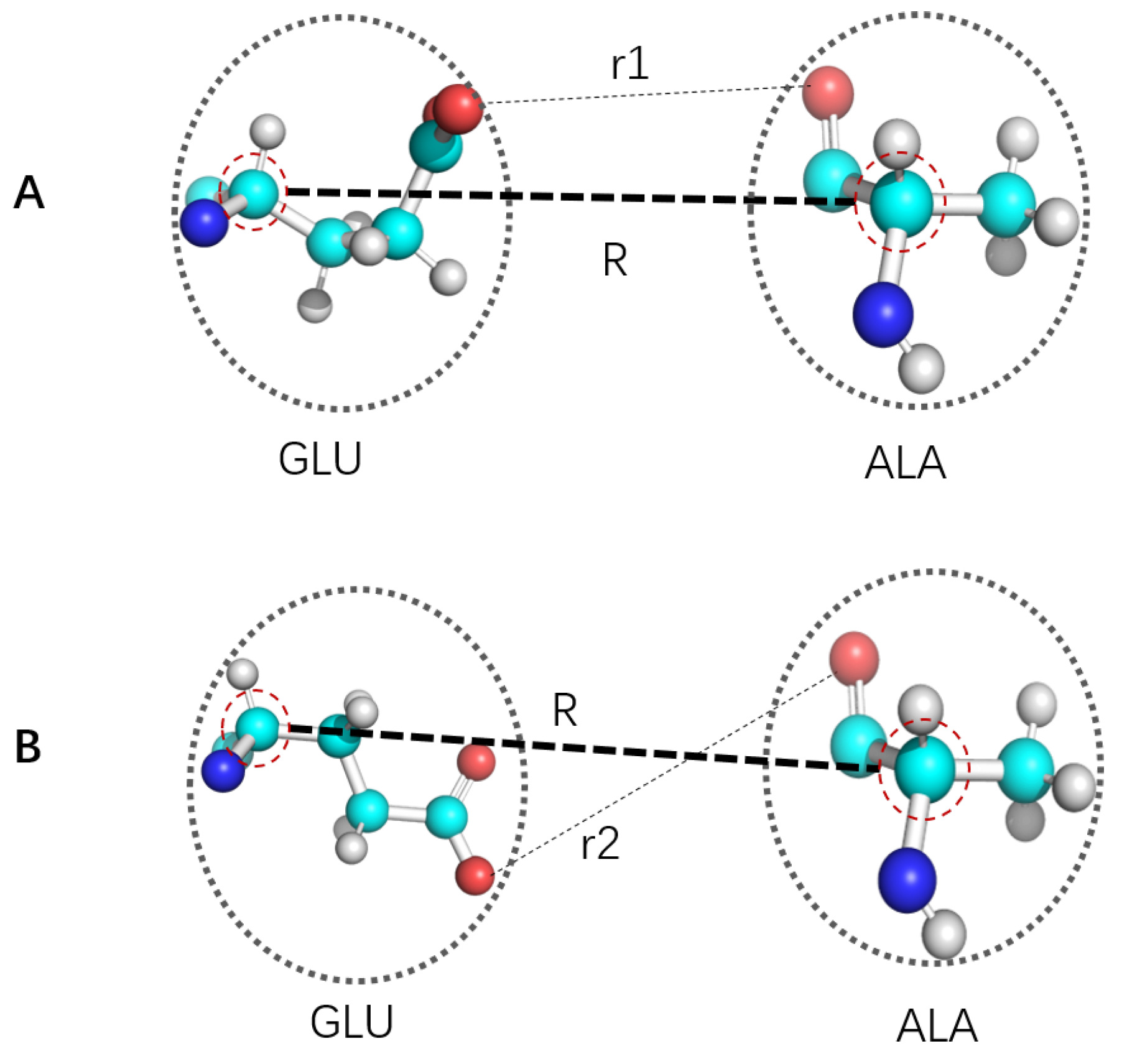
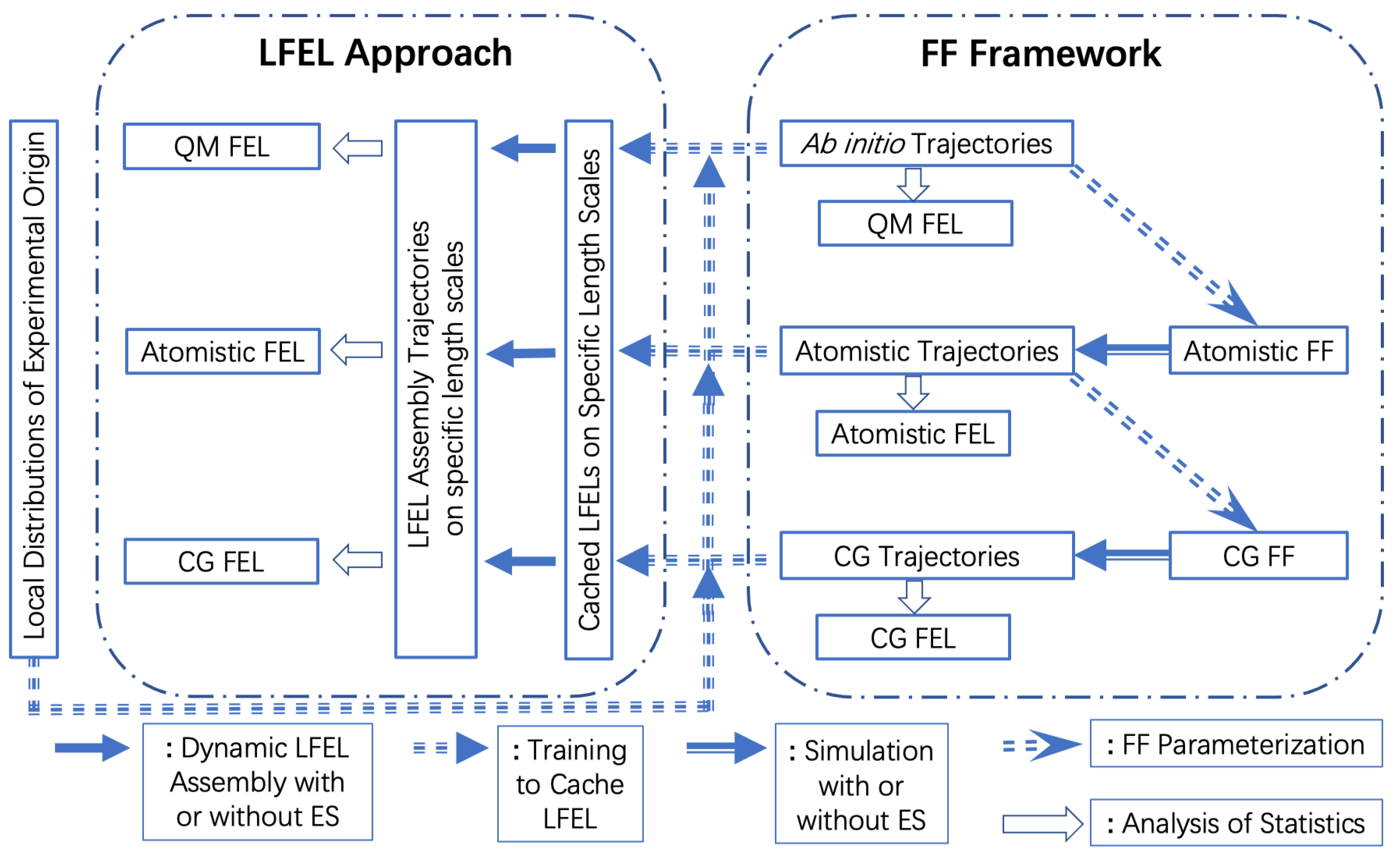
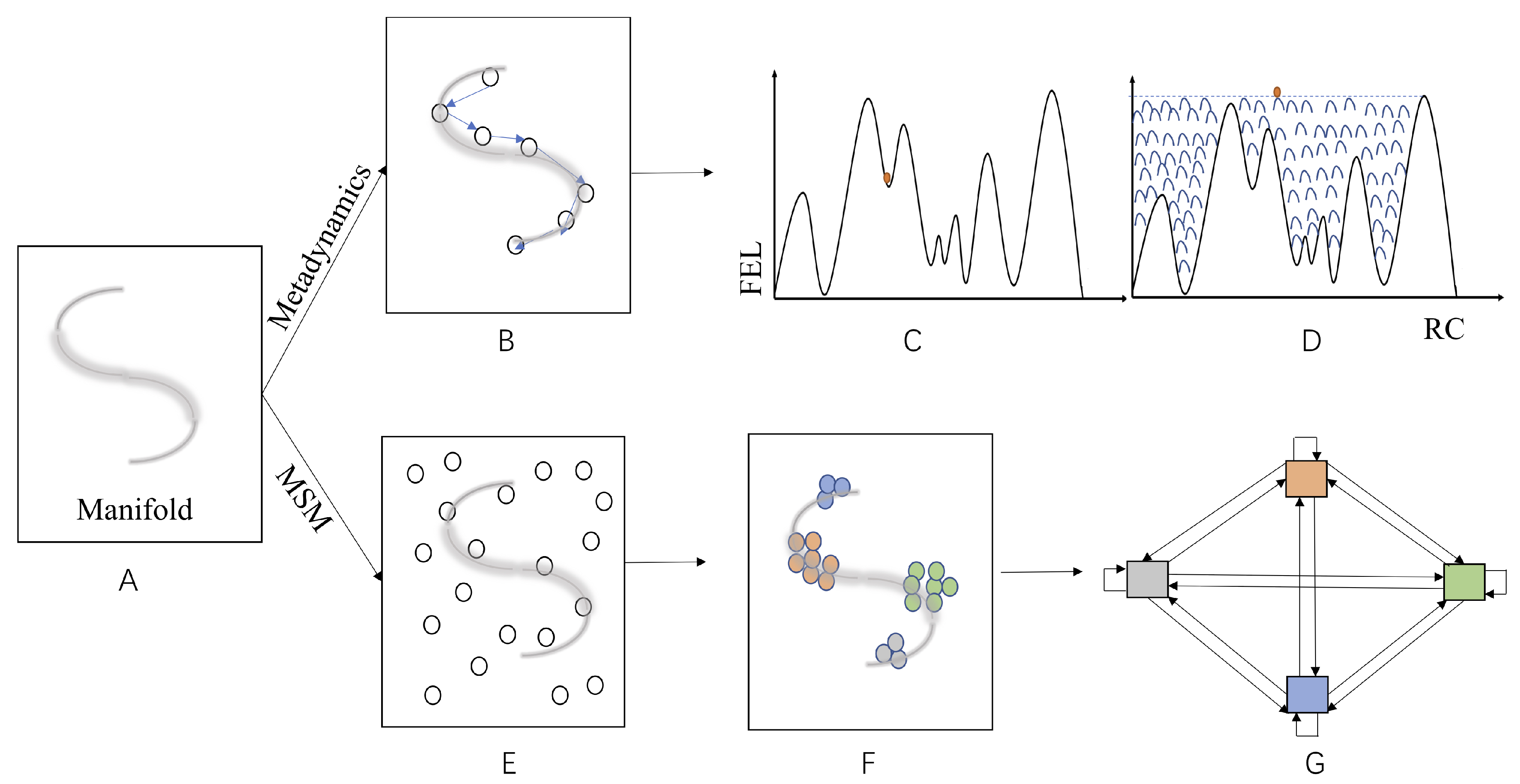
Table 1.
Number of publications from Web of Science search on 8 September 2020.
| Key Words | Number of Publications |
|---|---|
| Molecular dynamics simulation | 241,748 |
| Monte Carlo simulation | 189,550 |
| QM-MM (quantum mechanical—molecular mechanical) simulation | 9907 |
| Dissipative particle dynamics simulation | 3693 |
| Langevin dynamics simulation | 3893 |
| Molecular modeling | 2,072,091 |
| All of the above | 2,243,182 |
Table 2.
Commonality and difference among three types of algorithms.
| Algorithm | Coarse Graining | Enhanced Sampling | LFEL Approach |
|---|---|---|---|
| Resolution | Lower | In | In |
| Transferable? | Partial | No | Partial |
| Dividing space | Physical | Configurational | Physical |
| Free energy unit | Partially Specified | Specified | Arbitrary |
Publisher’s Note: MDPI stays neutral with regard to jurisdictional claims in published maps and institutional affiliations. |
© 2021 by the authors. Licensee MDPI, Basel, Switzerland. This article is an open access article distributed under the terms and conditions of the Creative Commons Attribution (CC BY) license (https://creativecommons.org/licenses/by/4.0/).
Share and Cite
MDPI and ACS Style
Cao, X.; Tian, P. “Dividing and Conquering” and “Caching” in Molecular Modeling. Int. J. Mol. Sci. 2021, 22, 5053. https://doi.org/10.3390/ijms22095053
AMA Style
Cao X, Tian P. “Dividing and Conquering” and “Caching” in Molecular Modeling. International Journal of Molecular Sciences. 2021; 22(9):5053. https://doi.org/10.3390/ijms22095053
Chicago/Turabian StyleCao, Xiaoyong, and Pu Tian. 2021. "“Dividing and Conquering” and “Caching” in Molecular Modeling" International Journal of Molecular Sciences 22, no. 9: 5053. https://doi.org/10.3390/ijms22095053
Note that from the first issue of 2016, this journal uses article numbers instead of page numbers. See further details here.