Article

Modeling Spatial Charging Demands Related to Electric Vehicles for Power Grid Planning Applications

1
Fraunhofer Institute for Energy Economics and Energy System Technology, 34119 Kassel, Germany
2
Department Integrated Energy Systems, University of Kassel, 34121 Kassel, Germany
*
Author to whom correspondence should be addressed.
ISPRS Int. J. Geo-Inf. 2020, 9(12), 699; https://doi.org/10.3390/ijgi9120699
Submission received: 20 October 2020 / Revised: 13 November 2020 / Accepted: 23 November 2020 / Published: 25 November 2020
(This article belongs to the Collection Spatial and Temporal Modelling of Renewable Energy Systems)

Abstract

:
The electrification of the transport sector together with an increasing share of renewable energies has the potential to reduce CO2 emissions significantly. This transformation requires the rollout of charging infrastructure, which has an impact on power grids. For grid planning and dimensioning purposes, it is crucial to assess this rapidly growing impact. We present an approach using socio-economic data such as income levels together with a model for demographic changes to estimate where electric mobility is likely to be concentrated, especially during the transformation phase. We present a total-cost-of-ownership approach for the ramp-up of electric mobility, considering an increased penetration of renewable energies. With the city of Wiesbaden in Germany as an example for an application area, the possible expansion of vehicle ownership and charging points is modeled on the level of individual buildings. Compared to a simpler approach, the detailed model results in more consistent charging point allocations, higher line/transformer loadings and lower bus voltages for the investigated grids. Predicting future distributions of charging points with such a level of detail in terms of ramp-up and spatial resolution proves potentially beneficial for grid analysis and planning purposes, especially in urban areas, where infrastructure changes are expensive and time-consuming.

1. Introduction

Electric vehicles can significantly contribute to a reduction of carbon emissions in the mobility sector. This transformation will be very dynamic, which poses a technical and economic challenge. The necessary charging infrastructure is a new element in our energy systems, which will have to be integrated into electric grids. Therefore, spatial modeling of future charging behavior is essential. An important area of application is grid planning as challenges may arise especially in distribution grids.
Modern approaches provide numerous methods of estimating the future spatial distribution of electrical generators and loads in the context of grid studies [1]. Criteria for spatial distributions can be based on probabilistic methods (e.g., wind energy in [2,3]), general siting suitability (e.g., photovoltaics in [2]) or prioritization [4,5]. In many studies, a spatial allocation at a higher level (e.g., municipal level) is carried out before a fine spatial distribution takes place [2,4,6,7,8]. The reasons presented for this two-step approach are increased robustness of the distributions and the option of using different allocation criteria at different levels [1,2,4]. The broad landscape of studies and methods for the spatial distribution of electrical power generation and electric loads is more limited when it comes to the distribution of electric vehicles and their charging points. There are fairly general allocation models based on population or vehicle distribution in general [2,9,10]. Various more detailed studies focus on public charging infrastructure, even if their concrete focus of investigation varies. Some of these studies, for example, [11], concentrate on fast-charging stations and a distribution based on optimization algorithms in order to assess those stations’ influences on the power grid. Another field of research is the differentiation between charging types and their optimal deployment [12]. Some studies have specific applications such as the optimal distribution across American state roads [13]. Numerous methodologies, such as the cross-entropy method [14] or agent-based models [15], are used to achieve an optimization of certain model variables. Furthermore, the target or evaluation size considered varies: while some studies address consumer costs for optimal placement [16,17], others explicitly consider environmental costs [18,19]. The studies have been developed partly in the context of providing concrete designs for planned charging point expansions [20,21].
There are grid integration studies that examine electric mobility by means of probabilistic allocations of charging points with a high level of spatial resolution [2] or scenario data based on population and market research data [22]. However, these two scenario aspects are not combined in previous research and there are no analyses about which level of spatial resolution is most suitable for grid planning applications in (urban) low-voltage grids.
The aim of this work is to establish a method that generates possible future distributions of electric vehicles and to investigate their impact on grid planning through domestic charging stations. This paper differs from many state-of-the-art publications in that it does not aim to optimize the distribution of charging points but to depict plausible developments based on a probabilistic approach. For example, this method could be used to determine the expected costs of necessary grid expansion and is thus a small building block in paving the way for the energy transition. The availability of a method for a possible distribution of home charging stations with a broad applicability in Germany can advance research and the industry (especially distribution network operators) and allow for more accurate cost estimation for grid reinforcement. It is not in competition with optimization models but represents a different field of application.
This paper presents and evaluates the following hypothesis: detailed models for the spatial allocation of charging points considering socio-economic attributes are beneficial for power grid planning purposes.
Section 2 presents our methods for generating high-resolution charging point distributions and how they can be used in power grid calculations. In Section 3, the results of the application of these methods are presented based on a case study for the city of Wiesbaden in the year 2040. Section 4 discusses the applicability but also the limits of the methodology and how it could be expanded and further developed in the future. Furthermore, the validation of the hypothesis from the beginning of this paragraph is discussed in Section 4.

2. Materials and Methods

In this section, we present our approach, which consists of the following steps: first, a nationwide vehicle fleet is modeled. After that, demographic change and the expected number of charging points are modeled on a municipal level. Based on these results, high-resolution distributions of charging points are determined considering population properties like income or age. Finally, the impact of the expected charging point distribution on the existing power grid infrastructure is examined. Figure 1 presents an overview of the components of our model. Each component is described in a subsequent subsection.

2.1. Methods: Vehicle Fleet Modeling for Germany

In this section, the methods to create a vehicle fleet composition in the target year 2040 including electric vehicles is presented. In [23,24], a model to quantitatively determine future vehicle fleets was developed that considers a variety of technical, ecological and economic input parameters and allows for a detailed simulation of the market penetration of different types of electric vehicles. The model is summarized below, and a schematic overview is shown in Figure 2. The general idea is to calculate the changes in the vehicle fleet over time for the coming years at a yearly resolution.
The first step is to initialize the model by a defined vehicle fleet (e.g., a representative vehicle mix consisting of 67% gasoline cars and 33% diesel cars across the small and medium segment). Building on the initial vehicle fleet, the yearly turnover in the fleet is calculated. Vehicles leave the fleet because of damage or age, and newly purchased vehicles are added.
The modeling approach is based on a bottom-up consumer demand model combined with dynamic stock modeling. As a central element, the individual purchase decision is based on the difference in total cost of ownership (TCO) of the considered vehicle types. For this purpose, all foreseeable costs for vehicle use are calculated for a specific holding period or vehicle lifetime and transformed into specific costs per kilometer. A distinction is made between private and commercial customers in terms of holding period, interest rate and possibility of a value-added tax refund [23,24].
To take into consideration updated data and the focus on electric vehicles for this work, the model from [23,24] has been adjusted as follows:
  • Updated policy trends, including a faster increase of the CO2 price and a faster reduction of the feed-in tariff (see Appendix A, Table A1 for specific values)
  • Added parameter “car rank” in order to distinguish between a household’s first car and second car. The type of vehicle use varies for the parameter (e.g., no long-distance travel for second cars, which represent almost 25% of all registered cars in Germany [25]) and thus the boundary conditions, for example, for battery range (see Appendix A, Table A3)
  • New regulatory framework, described in [26], with differentiated price forecasts for every consumer group in all energy sectors, including the energy industry, general industry, residential and commercial buildings and the transport sector
  • Updated starting point for the simulations to 2018 due to availability of data [27]
  • Updated vehicle component costs (see Appendix A, Table A2) and battery capacities (Table A3)
The outcome of this vehicle modeling approach is the expected composition of the nation-wide vehicle fleet in the relevant years and thus forms an input for creating regionalized vehicle and charging point figures at the municipal level.

2.2. Methods: Municipal Level

The goal of the next step is to regionalize the expected nationwide numbers of electric vehicles at the municipal level. However, besides the vehicle fleet, a second central basis is to take into account changes in the population structure for future scenarios (Section 2.2.1). Demographic change has, among others, an influence on the number of charging points per municipality (Section 2.2.2).

2.2.1. Methods: Demographic Change

We use a forecast of demographic change until 2030 by the Bertelsmann Foundation [28]. The forecast includes population projections for municipalities with more than 5000 inhabitants. To display the development from 2030 to 2040, a demographic model has been established that takes into account the following annual changes throughout the municipalities:
  • Birth: number of births, depending on the number of women potentially giving birth in the age group of 15–49 [29]
  • Death: mortality rates per age [30]
  • Migration: taking into account the migration factors of the years 2016 and 2017 by age group in each municipality [31]
The future population of municipalities with less than 5000 inhabitants is estimated based on the projected population size of the district. After the per-district processing of the population data, the size of the individual municipalities is determined proportionally, based on the population distribution in the year 2017 [32].
In order to avoid outliers in the overall development through extreme migration over the model years, the overall growth compared to 2017 is limited to the 1–99% quantile. In Section 3.2.1, the applicability and its limits are discussed. The modeled demographic change serves as an input for two other parts of our model: charging points per municipality (Section 2.2.2) and building-specific household modeling (Section 2.3.1).

2.2.2. Methods: Charging Points per Municipality

In the first step, we determine the number of electric vehicles at the municipal level with a methodology that was developed within the framework of the Verteilnetzstudie Hessen (Distribution Grid Study Hesse) [2]. In the second step, these numbers are used to determine the number of domestic charging points needed for these electric vehicles.
The classic top-down allocation procedure distributes an initial variable (electric vehicles from the scenario framework) to a lower level (municipalities) using a distribution variable. The distribution variable is made up of the number of inhabitants and various other factors. In order to take into account updated data and further development of the methodology, the following adjustments have been made compared to the above source:
  • Vehicle fleet figures have been adjusted and extended to cover a longer period (until 2040)
  • Distribution factors: adjustment of the influence of commuters since a scenario further in the future is described in which their influence decreases (damping the original factor of [2]); new inclusion of demographic change (see Section 2.2.1); new inclusion of registered vehicles per municipality in consideration of structural and geographical modal-split characteristics; and updated input data for residents [33] and commuters [34]
  • The conversion between vehicles and charging points is updated to use a new factor of 0.7, which is based on [35] and defined as the base case in the project consortium of Ladeinfrastruktur 2.0 [36].
The number of vehicles is thus determined—in analogy to [2] and with the changes mentioned above—based on the following equation:
n cp ,   j = f cp / ev × n ev ,   j = f cp / ev × I j × f demogr ,   j × f v / inh ,   j   × f com ,   j i ( I i × f demogr ,   i × f v / inh ,   i   × f com ,   i ) × n ev ,   national ,
where:
j: considered municipality; i: all municipalities; ncp: number of charging points; fcp/ev: charging points per electric vehicle; nev: number of electric vehicles; I: inhabitants; fdemogr: demographic-change factor; fv/inh: registered vehicles (including combustion vehicles) per inhabitant and fcom: commuters factor.
The definition of the factors is used as a base case. The benefit of this methodology is that it can be updated with newer input data and findings. The number of charging points refers to domestic charging points.

2.3. Methods: Household Level

Based on demographic change (Section 2.2.1) and the number of charging points per municipality (Section 2.2.2), the high-resolution, house-specific population structure and a possible distribution of vehicles and—in a second step—charging points is modeled. These high-resolution scenarios will be calculated in different allocation variants (the same boundary conditions but different random samples) to allow for a probabilistic power grid calculation (Section 2.4). Additionally, sensitivities (changed boundary conditions) provide an opportunity to investigate the influence of variables.

2.3.1. Methods: Population Structure

The spatial distribution of charging points is based on population structure data. To generate household-exact data, it is necessary to know the positions of households and their characteristics. Relevant data is only available at a higher and aggregated level for now. For that reason, we have developed a model for creating representative individual households that also includes their positions. The model is based on a dataset that contains household data aggregated by street sections and a wide range of socio-economic characteristics provided by GfK Geomarketing [33]. In the German city of Wiesbaden, a street section comprises almost 28 households on average, and, in the areas most relevant in this application (city areas), a street section usually extends to only a few buildings due to a high number of street crossings. Single outliers of larger groups of households are rare. The street section with the maximum number of households contains large apartment blocks on the outskirts of the city with a homogeneous building structure. However, the data is stated as marginal sums for the respective street and needs a methodology for allocation to individual households so scenarios for a point-precise distribution of charging points to addresses rather than street sections can be created. This synthetic population is created using the iterative proportional fitting algorithm [37] for the characteristics of income and household type. Age, sex and the number of inhabitants per household are assigned using a random weighted distribution based on statistical data of the German Federal Statistical Office [38,39]. We wish to emphasize that we do not assume that the resulting household data matches the actual household distribution of any individual household but does adequately reflect the population for the question at hand (distribution of charging points).
In order to take into account the demographic change until 2040, households will be added or removed, based on the development of age in the municipality (see Section 2.2.1). As an assumption, the household attributes of added households are taken from the previous average, differentiated by age.
An example for both assumptions is given in Appendix B. The number of households of each age group can increase or decrease in the future. A number of households of the type subject to a decrease is randomly chosen and removed from the datasets of the relevant age groups. In case the number of households of other age groups increases, the removed households are replaced. If available, additional households can be assigned to new development areas in the study area. For the area of Wiesbaden, addressed in this paper, this kind of data was not available. According to our assumption, the additional households are accounted for by redensification and randomly placed in the existing street sections, with street sections that currently have a high number of inhabitants being more likely to receive additional households.
After the household dataset for the scenario year 2040 and each street section has been created, the households are placed at exact geographic locations (i.e., buildings and their addresses). For the assignment of buildings to addresses, a dataset is used that assigns addresses to streets by means of string comparison using the Levenshtein distance from the street name [40]. The living space per building is determined based on the floor area and height of the building [41], and the households are distributed proportionally. To determine which household is placed in which building, a weighted random distribution is applied based on data from the German Federal Statistical Office relating to household types and buildings [42].

2.3.2. Methods: Charging Point Allocation

In this section, we explain how we proceed from charging points per municipality (Section 2.2.2) and a high-resolution population structure (Section 2.3.1) towards a possible allocation of charging points in a municipality.
The process uses the following steps: first, several criteria are combined in a utility value analysis [43], which models the probabilities of purchasing an electric vehicle for the individual households. Second, a sample for an allocation of electrical vehicles to households is drawn from the resulting probability distribution. Third, a probability for these vehicles to receive a charging point is modeled. Last, a sample of charging points is drawn. This process is depicted in Figure 3, followed by a more detailed explanation of the methodology.
In the following, the individual steps are explained in detail, starting with the question of how to derive criteria for electric vehicles from a population structure. Various sources indicate a more likely purchase decision for electric vehicles in households with certain characteristics [25,44,45]. We use a method analogous to a utility value analysis to apply a score to households. Table 1 shows the criteria (with their respective weighting in the overall score) and their different specifications (with the respective scores). The weightings have been determined by various experts in the project team as plausible starting values and are investigated using a sensitivity analysis (see Section 3.3.2 and Appendix C). The scoring is based on the characteristics of electric-vehicle buyers—that is, for example, the fact that first-time users of electric vehicles have a high income and are predominantly male [25,44,45]. Based on the scoring model, each household gets a specific score depending on the individual household characteristics. We wish to emphasize the fact that weightings and scorings can be varied if new findings become available.
As an example, a multi-person household without children (15% × 8 = 1.2) in a two-family house (40% × 7 = 2.8) with an income above 4000 € (40% × 9 = 3.6) and a female main wage earner (5% × 1 = 0.05) would receive an overall score of 1.2 + 2.8 + 3.6 + 0.05 = 7.65.
The higher the score, the higher the likelihood is of that household acquiring an electric vehicle.
In general, a wide range of options are available for combining different properties and reducing them to one parameter. We have chosen an additive method analogous to a utility value analysis for the following reasons:
  • A multiplicative method would require independent variables (e.g., income without interdependence on household type) to be known, which is rarely the case for statistical statements on purchasing behavior.
  • A clearly defined probability for a purchase decision does not appear to be determinable for the actual complex problem. It is rather a matter of comparing different households, which corresponds to the objective of a utility value analysis
In an iterative process, vehicles are distributed to households until all vehicles per municipality have been distributed. The number of sampled vehicles is limited to one vehicle per single household and two vehicles per multi-person household.
In a second step, charging points are distributed. Each household with an electric vehicle can get one charging point per vehicle, and the likelihood of assigning a charging point to a vehicle depends exclusively on the building type. This process is repeated 50 times to achieve a variety of possible charging point distributions, which allows for probabilistic modeling of grid calculations.
In summary, the methodology is characterized in particular by the following features:
  • Mapping of household characteristics
  • A variety of possible charging point distributions
  • Suitability for sensitivity analysis
  • Exact spatial distribution, which enables a precise allocation to house connections
For a complete and detailed grid analysis, other types of charging points as well as other generation and load types can be considered to get a more accurate picture of the impact on the grid. Other generation and consumer types have been modeled in [2]. One example are photovoltaic systems, which are sized and allocated based on scenario targets and potentially available areas and whose feed-in time series are calculated using irradiation-based satellite data [46]. Another example is heat pumps, which are allocated based on size classes and applications regarding the distribution between residential and commercial buildings and average mixes of plausible size classes. These producers and consumers can be taken into account for grid planning applications. To simplify the analysis, the grid analysis in this paper is limited to charging points.

2.4. Methods: Grid Calculation

As outlined in the previous section, we can determine a possible spatial allocation of charging points in a defined area. What remains to be determined is the impact of these charging points on the power grid. When power is drained from the electrical grid, two things happen. First, the voltage around that point in the grid drops, and second, the loading of the power line(s) leading from the transformer station to the point increases due to the additional current. For a high number of simultaneous charging processes, these effects can accumulate and lead to violations of the minimal-voltage requirement or to the overloading of either lines, transformers, or both.
In the following, we demonstrate how we use the derived spatial allocation of charging points to assess worst-case situations that might realistically occur in distribution grids caused by charging vehicles. Additionally, we present an approach to evaluate the influence of the level of detail in our model for spatial allocation of charging points on those worst-case assessments.

2.4.1. Charging Point Grid Integration

Up to this point, the spatial allocation of charging points has been carried out completely independently of any information about the power grids they are connected to. However, in order to assess the impact of the charging infrastructure, we need to determine the exact connection point to the underlying power grid. Domestic charging points—as considered in this paper—are assumed to be attached to the low-voltage connection point of the buildings they belong to. For this reason, we assign each charging point to the closest low-voltage connection point within a radius of 30 m. This cut-off distance is necessary to prevent the assignment of a charging point to a building it is too far away from. For each grid, this process is carried out for 50 probabilistic spatial charging point allocations. This is of central importance as an analysis of a variety of possible charging point allocations provides a more robust indication whether problems are likely to occur in a grid or not than a result based on a single allocation.
As shown in the sections above, our model for spatial allocation relies on various sources of statistical, geographic and demographic information. As stated in the hypothesis (Section 1), we wish to investigate if detailed models for the spatial allocation of charging points are beneficial for power grid planning purposes. In order to do so, we aim to evaluate if this very detailed model results in different worst-case assessments than simpler approaches. For that purpose, we perform the same grid simulations based on three allocation approaches with different levels of complexity:
  • Allocation per household considering household attributes: charging points are allocated to households according to their overall scores (see Section 2.3.2). Households with higher scores are more likely to receive charging points. This is the detailed approach presented in Section 2.3.
  • Allocation per household ignoring household attributes: all charging points are allocated to random households, pretending that the method presented in Section 2.3.2 was not available.
  • Allocation per street section considering household attributes: charging points of buildings in the same street section are aggregated at the street center level instead of that of individual buildings. All household attributes are considered as presented in Section 2.3.2.
For all three allocation approaches, the number of charging points per municipality is identical. The simplifications represent real-world grid planning processes, where the availability of non-grid-related information is usually very limited. The result of this allocation process is 50 spatial allocation variants per allocation approach.

2.4.2. Worst-Case Assessment

After the allocation of charging points, we know how many charging points are connected to a specific grid at what location. As a result, we also know the hypothetical maximum power flow that would occur in that grid if all charging points were used at exactly the same time. In reality, however, this situation is highly unlikely. Therefore, the next step in assessing worst-case grid situations is to determine the realistic maximum simultaneous power flow caused by charging vehicles. This is nontrivial since the relation between the number of charging points and the resulting maximum power demand is nonlinear: with an increasing number of charging points, the additional worst-case power flow decreases. The more charging points are connected to a grid, the less likely it is that they will be used simultaneously. In grid planning, this fact is taken into account by using simultaneity factors. A simultaneity factor for n consumers or producers is the ratio between the sum of their maximum simultaneous power flows and the sum of all individual peak power flows:
f simultaneity , n =   i = 1 n max .   simultaneous   power   flow i i = 1 n max .   individual   power   flow i .
When this factor is determined for different values of n, the result is a simultaneity curve that can be used to quickly obtain simultaneity factors for any number of charging points. Figure 4 shows the simultaneity factors for any number of 11-kW charging points from 1 to 10,000. The simultaneity curves we use in this paper are calculated based on simulated charging profiles. The method is described in [47].
The combination of charging point allocations and simultaneity factors allows us to calculate the worst-case voltages and power line/transformer loadings for all 62 grid models. All grid calculations are performed with pandapower [48,49], an open-source grid modeling, analysis and optimization software. Since we consider 50 variants of spatial charging point allocation per grid, we obtain 50 different grid calculation results. In order to compare the different allocation approaches (see Section 2.4.1), we determine the median bus voltage, line loading and transformer loading of 50 simulations for every bus, line and transformer per grid. These median values represent the expectable worst-case results and allow us to evaluate whether different allocation methods lead to different worst-case assessments or not.

3. Results

This section is structured in analogy to the methods section, following the same subsections (see Figure 1). The results of vehicle fleet modeling (Section 3.1), demographic change and the number of charging points at municipal level (Section 3.2), the fine-scale, household-related distributions (Section 3.3) and the grid calculation (Section 3.4) are discussed.

3.1. Results: Vehicle Fleet Modeling for Germany

The vehicle fleet model (see Section 2.1) for Germany has been determined based on the assumptions of Table A1, Table A2 and Table A3. It was run with 20,000 vehicles representative of the German vehicle fleet.
The results of the simulation showed a market ramp-up of electric vehicles (see Figure 5). The share of electric vehicles will increase from today’s 0.3% of the total German vehicle fleet to 16.2% in 2030, on to more than 52% in 2040 and, finally, to more than 80% in the long-term perspective (see Table 2).
More progressive assumptions (the reform scenario as shown in Table A1) resulted in a much faster market uptake of electric vehicles, so that electric vehicles (EVs) accounted for 24% (11.68 million EVs) of the total German vehicle market in 2030 and a penetration rate of over 90% in the long-term perspective. The results of 2030 meet the minimum target of the German federal government [51].

3.2. Results: Municipal Level

Together with the scenario framework, modeling at the municipal level forms the basis for a detailed modeling of charging points. Demographic change (Section 3.2.1) and the number of charging points (Section 3.2.2) are presented in this section for the Wiesbaden application area.

3.2.1. Results: Demographic Change

The application of the methodology for demographic change presented in Section 2.2.1 shows a plausible change in the population for most municipalities in Germany (see Figure 6a).
Particularly for the specific detailed consideration of small municipalities, an expansion of the input data on migration would be very helpful but is currently hampered by the inconsistent data situation [29]. The model appears valid for application to the example area of Wiesbaden and produces the population distribution shown in Figure 6b. Wiesbaden thus shows a predicted population increase of 4% by 2040, compared to the average development in Germany of –6%.

3.2.2. Results: Charging Points per Municipality

The methods described in Section 2.2.2 are applicable to every municipality in Germany. The figures for the municipality of Wiesbaden are presented in Table 3 and compared to nationwide average figures.
For Wiesbaden, the value for electric vehicles per inhabitant is close to the German average, due to close-to-average or mutually offsetting values (a growing municipality but low commuter and vehicle registration figures).

3.3. Results: Household Level

Application of the methodology presented in Section 2.3 provides a building-specific household structure, including changes due to demographic change (Section 3.3.1) and charging point allocations (Section 3.3.2). The calculation of 50 allocation variants of charging points makes a probabilistic grid planning approach possible (see Section 3.4). In this article, individual areas in Wiesbaden are presented as application areas.

3.3.1. Results: Population Structure

Based on street section population structure data [33] and the model for demographic change, the potential population for the year 2040 is determined for each household. The data—which can be determined for all municipalities in Germany according to the methodology described in Section 2.3.1—is presented here for Wiesbaden. For all 141,860 individual households, combinations of attributes (like income, household type, etc.) are assigned. An example is provided in Figure 7. Furthermore, there are additional households due to demographic change, a total of 5437 in Wiesbaden.
The data on the household-specific population distribution is used to determine possible charging point distributions as described in the next subsection.

3.3.2. Results: Charging Point Allocation

The distribution of household attributes (see Section 3.3.1) and the utility analysis presented in the methodology section (Section 2.3.2) yield results in the form of a score per individual household (see Figure 8a). The score is used for the repeated allocation of electric vehicles, which is shown for 1 of the 50 variants in Figure 8b. The scoring for the distribution of charging points (exclusively dependent on the building type, not shown separately) results in the distribution of charging points (Figure 8c), again for 1 of the 50 variants.

3.4. Results: Grid Calculation

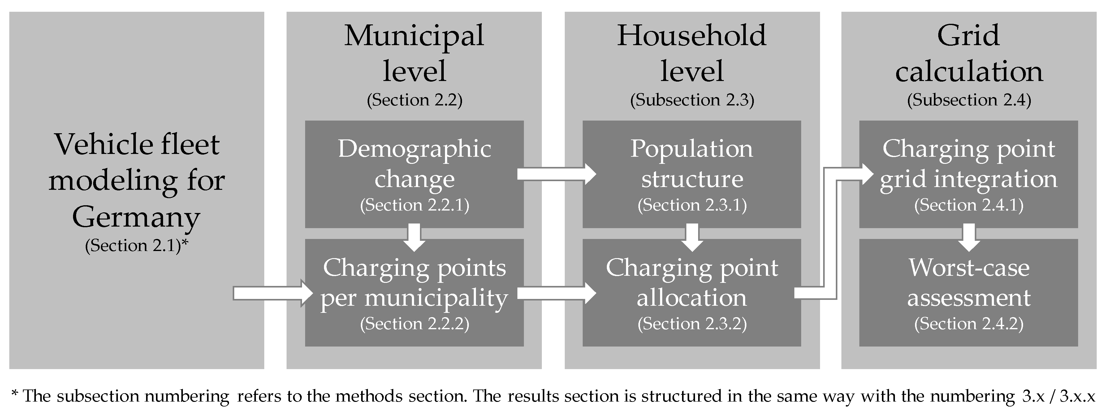
In this subsection, the charging point allocations presented in Section 3.3 are used to assess their impact on the underlying low-voltage grids. To this end, the charging points are integrated into the grid models as described in Section 2.4.1. Finally, by means of a power flow calculation, we determine the worst-case grid situations based on simultaneity factors according to Section 2.4.2. All these steps are performed for 62 real low-voltage grids and 50 spatial charging point allocation variants. The key result of this subsection is a comparison of three different levels of detail in spatial charging point allocation and the consequences for grid planning applications.

3.4.1. Results: Charging Point Grid Integration

In the following, we show the results based on the three charging point allocation approaches for a specific low-voltage grid. Additionally, we analyze how the number of allocated charging points in the same grids differs between the approaches. 
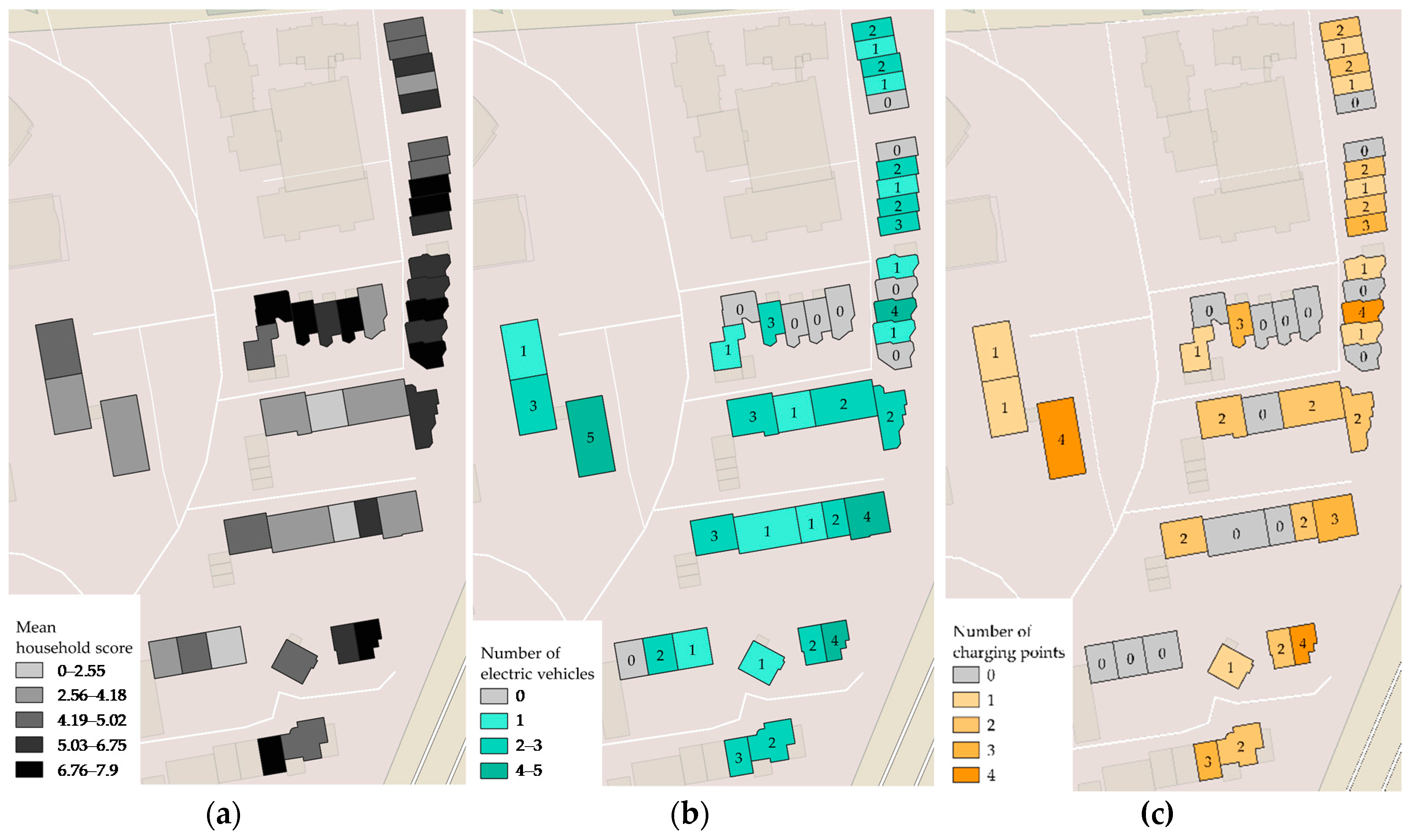
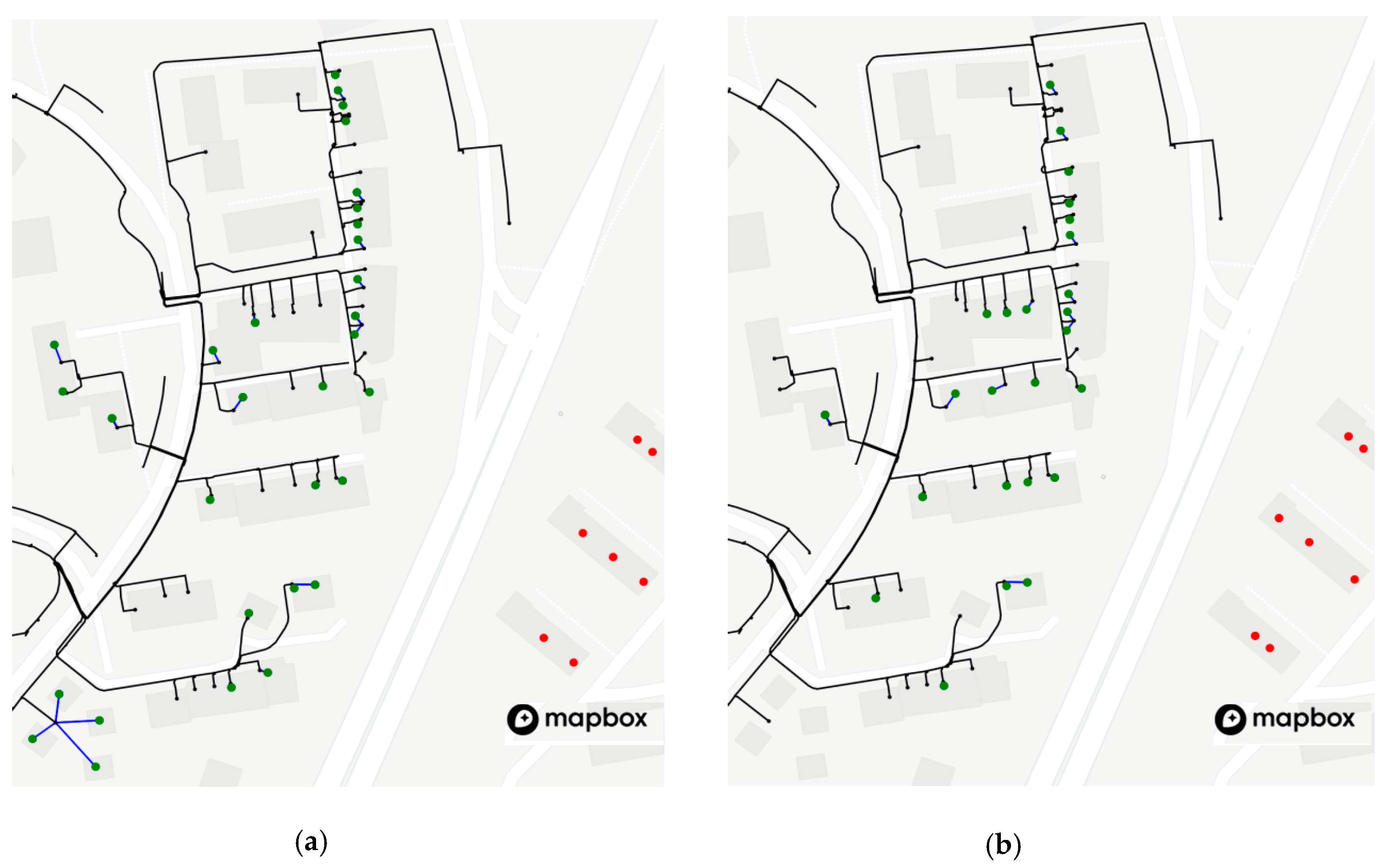
Figure 9 shows a section of a low-voltage grid combined with the same charging point allocation as presented in Figure 8. Figure 9a is in analogy to Figure 8c. Green dots represent one or multiple charging points that are connected to the closest low-voltage connection point of a building. Red dots are charging points that are too far away from this specific grid. These charging points are very likely connected to a different low-voltage grid. This grid configuration considers all available information on the location of charging points. Figure 9b shows the grid integration of charging points without considering the detailed allocation model based on household attributes. Instead, charging points are assigned to randomly chosen low-voltage connection points, resulting in different spatial distributions of charging points. The total number of charging points per municipality that are allocated to individual households is the same as for the method considering household attributes. However, the number of charging points in a specific grid is not necessarily the same: if households’ attributes are considered, some households have a higher probability of being chosen than others. As a result, grids containing these kinds of households will receive, on average, more charging points compared to a random distribution where the probability is equal for all households. If the median numbers of charging points per grid between both allocation approaches are compared to each other, the results differ quite a lot: the approach with household attributes results, on average, in 14% more charging points that are added to the 62 low-voltage grids. The highest positive deviation regarding the median number of charging points per grid is 131% more charging points when considering household attributes compared to random distribution. The highest negative deviation amounts to 48% less charging points. This indicates that—at least for these 62 low-voltage grids—the consideration of household attributes has a big impact on the spatial distribution of charging points within a municipality and therefore is also an important factor of influence on grid planning results.
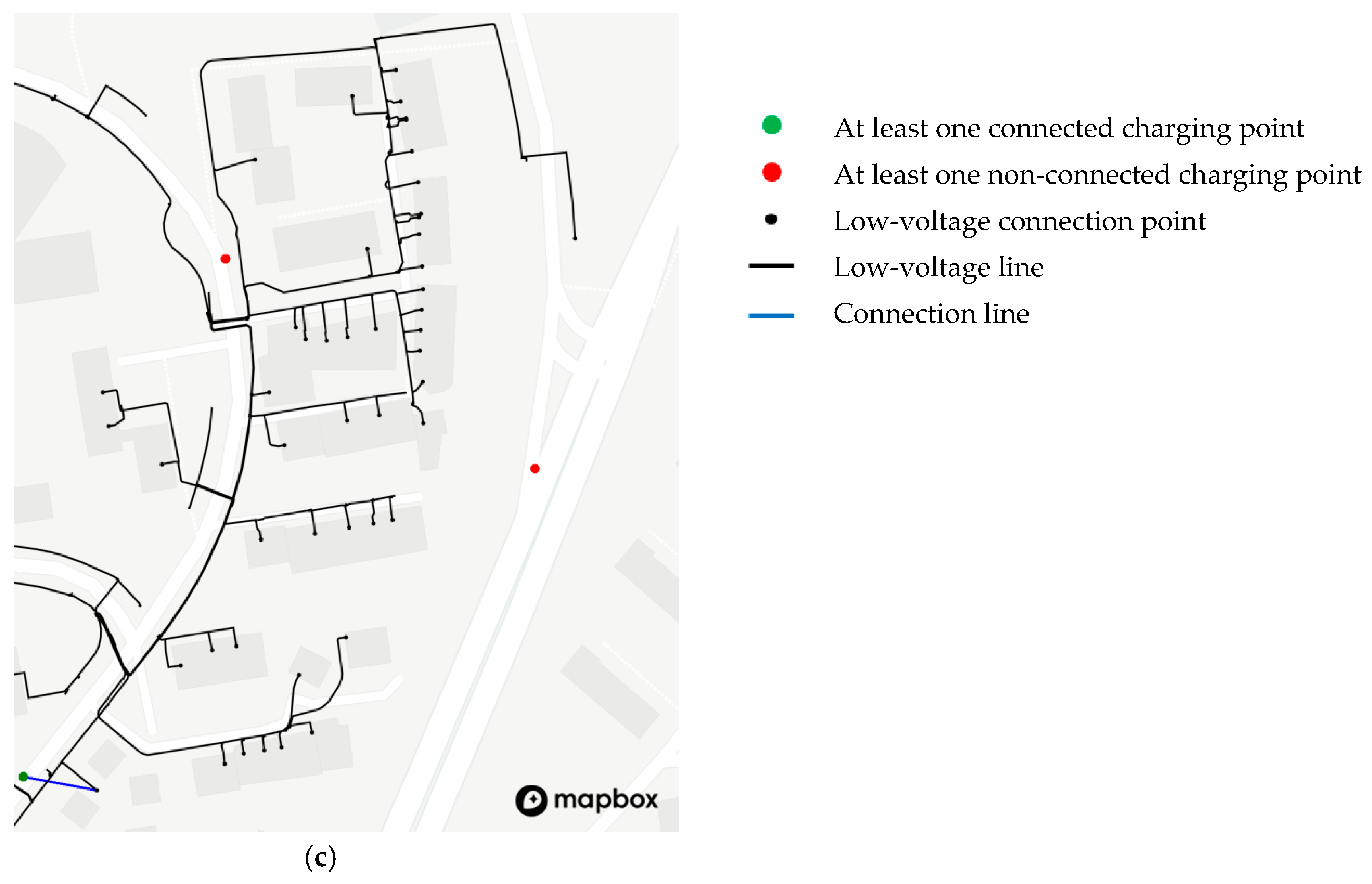
Figure 9c represents a case where all household attributes are considered but their spatial allocation is performed at a lower resolution: instead of placing charging points at individual buildings, all charging points in the same street section are aggregated at the center of that section. The number of charging points per street section is exactly the same as in Figure 9a. The example in Figure 9c, however, reveals an important issue with this allocation approach: only one of the two charging point locations in the left-hand part of the figure is connected to a low-voltage connection point. As indicated by its red color, the dot in the upper left-hand part of the image is not connected to any low-voltage connection point since there is no connection point within a 30-m radius. Increasing this radius is not a valid option either: if one did so, the red dot in the right-hand center area would be connected to this grid even though it represents charging points located at buildings that likely are supplied by a different low-voltage grid. This is not a cherry-picked example: only in 45 of 3100 charging point allocations (62 grids × 50 allocation variants) did the aggregated approach result in exactly the same number of charging points integrated into the grid. In the extreme cases, the lower spatial resolution leads to 500% more charging points or 100% less charging points compared to the more detailed allocation method. This issue especially occurs in urban areas, where low-voltage grids typically cover a relatively small area. Consequently, there is a high risk that charging points are assigned to the wrong grid if they are not allocated to specific buildings.
Based on these findings, the approach shown in Figure 9c cannot be recommended for grid planning purposes. For this type of use case, scenario allocations should not be aggregated before they are combined with grid data. A high degree of granularity in spatial allocation increases the likelihood that new producers and consumers are assigned to the correct low-voltage grids. Another central finding is that the consideration of household attributes leads to a significant shift of charging points from some grids to others compared to random distribution. However, a random-distribution approach is much easier to carry out, since it requires much less information. Therefore, in the following section, we will analyze to what degree neglecting household attributes affects grid calculation results.

3.4.2. Results: Worst-Case Assessment

The results of Section 3.4.1 indicate that a random distribution of charging points leads to significantly different numbers of allocated charging points per grid. In this section, we want to investigate to what degree the consideration of household attributes like income or building type is an important influence on grid planning results. Therefore, we compare the results of power flow calculations based on charging point allocation with and without consideration of household attributes as shown in Figure 9a,b. 
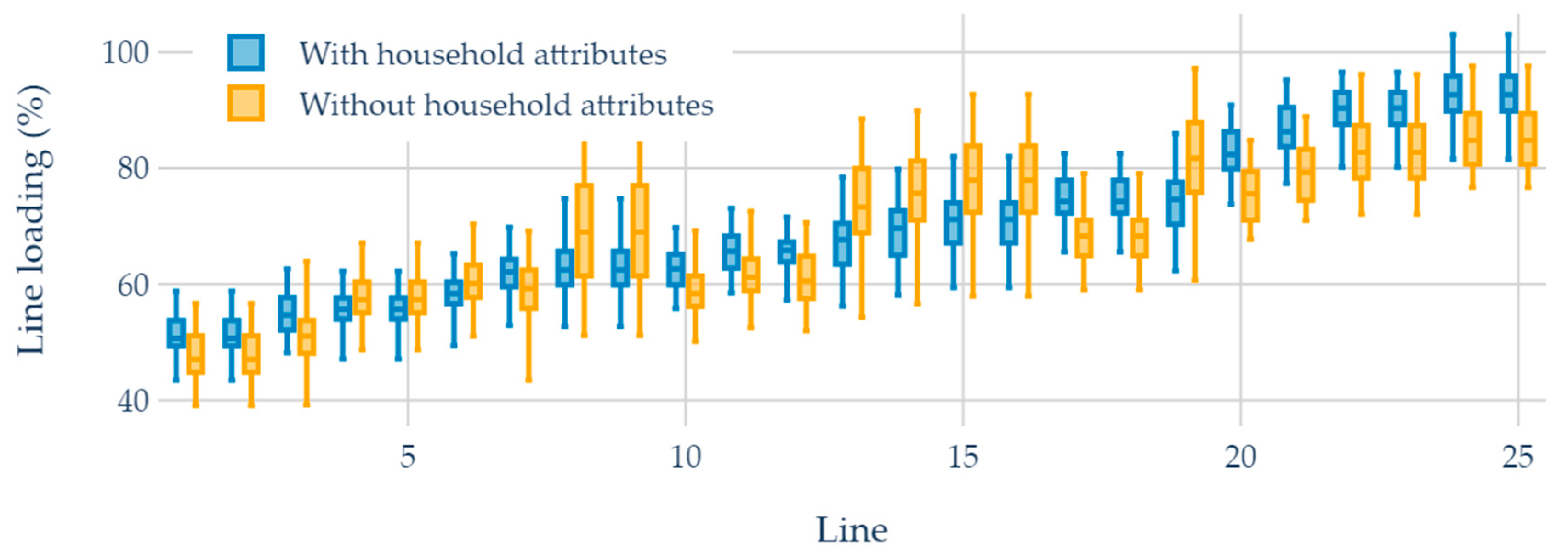
Figure 10 presents the line loadings of 25 lines for 50 charging point allocations variants for the same grid as presented in Figure 9. This subset was chosen because all of those lines have a median loading of over 50%. For grid planning purposes, grid elements that are closer to violating a technical limit are usually most important. The line loadings are visualized as boxplots, consisting of 50 data points each. The boxes mark the 25th/75th percentile and the median; the whiskers show the absolute minimum/maximum per line in 50 variants. The blue boxes represent the results based on an allocation with consideration of household attributes. The results presented in orange have been calculated without this information. At first, in order to analyze if there is an overall trend and to ignore outliers, we compare the median results based on the two different allocation approaches. The results for this subset of lines show slightly higher loadings when household attributes are considered. For 15 of 25 lines, the median line loading determined with consideration of household attributes is higher, for the remaining 10 lines it is significantly lower. In this case, there is not a single line where the median loading for both allocation approaches is on an equal level. However, it can be seen that the approach without consideration of household attributes results in a much higher spread of line loadings over the 50 charging point allocation variants. This is consistent with the findings of Section 3.4.1: for the approach without household attributes, there are much fewer constraints for the allocation of charging points, resulting in a higher variance of their spatial distribution. This also leads to a higher variance of line loading results.
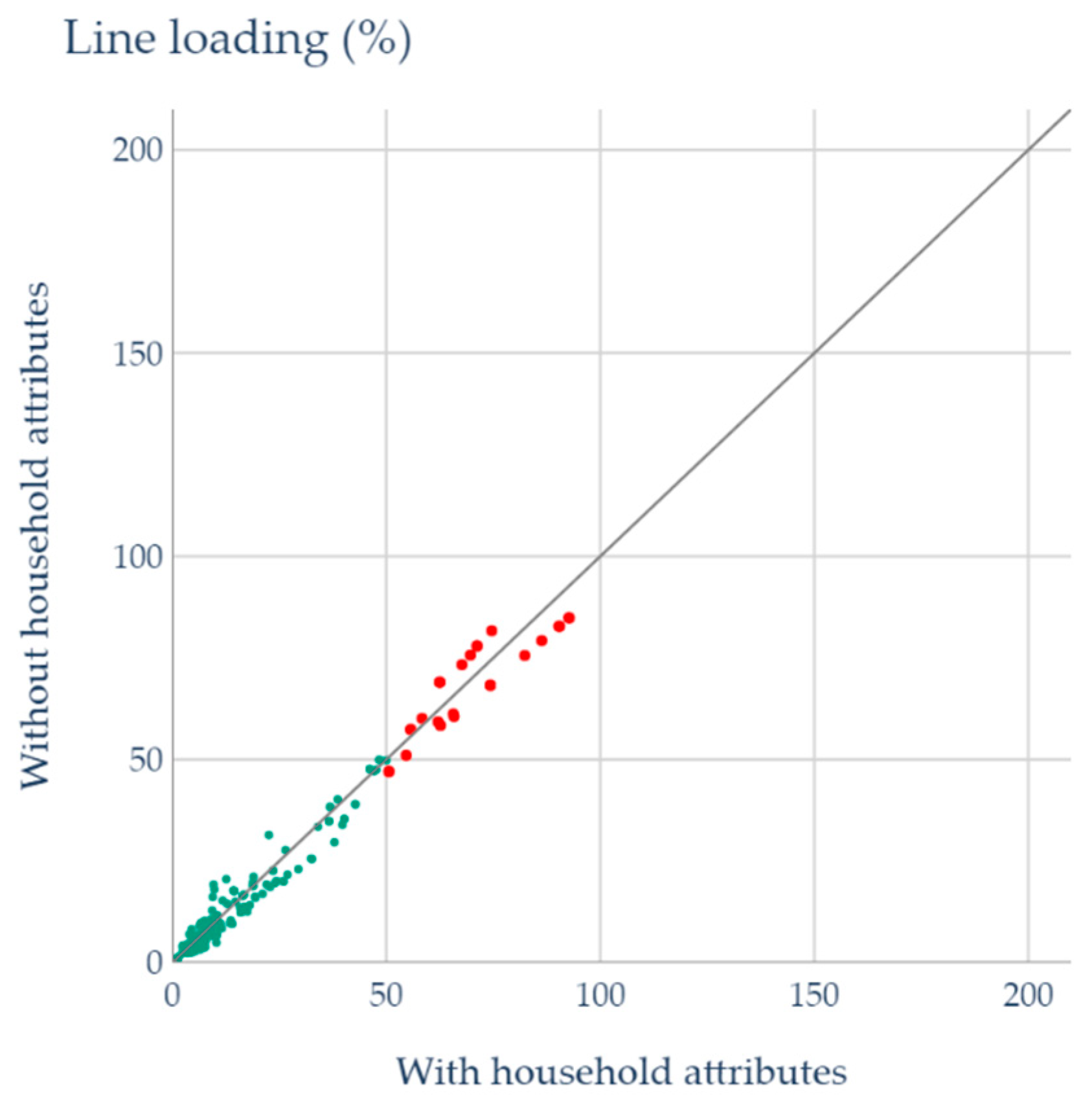
Figure 11 makes the line loading comparison in this grid easier to understand. Each dot in this figure represents the relation between the median line loads of a single line, determined with and without consideration of household attributes. The x-axis shows the results with consideration of household attributes, the y-axis the results without using this information. If a dot is located on the diagonal zero line, both results are identical. If it is located below the zero line, a charging point allocation with household attributes resulted in a higher median line loading and vice versa. The red dots show the medians of the same 25 lines as presented in Figure 10. The results are similar to those shown in Figure 10: for the majority of lines, considering household attributes results in higher median loadings. This is not just the case for the 25 lines marked in red but for all lines in the grid.
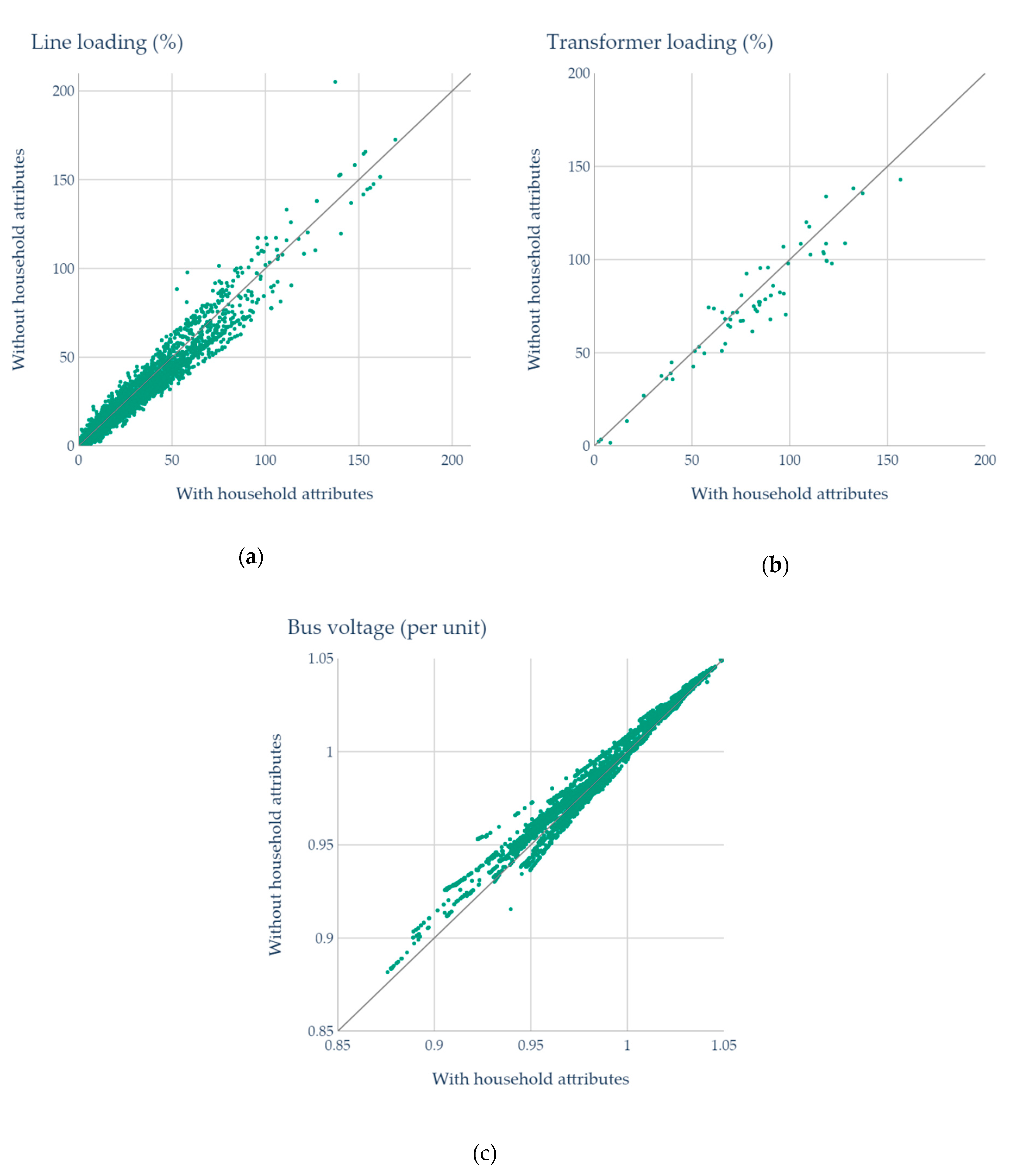
Figure 12a presents the same graph for the median loadings of all lines in all 62 low-voltage grids. The overall trend remains the same: the majority of median line loadings are higher if household attributes are considered. Additionally, the absolute deviation between both approaches increases for higher line loadings. The median transformer loadings presented in Figure 12b show a similar pattern. Since there is only one transformer per grid and all charging points in a grid directly increase transformer loading, these results deliver a comparison of the median worst-case power flows per grid: in 34 of 62 low-voltage grids, the approach with consideration of household attributes results in higher worst-case power flows. In 13 grids, the results are on a similar level and, in 15 grids, the approach without household attributes leads to higher power flows.
Figure 12c shows the same comparison for the median voltages of all low-voltage connection points in the 62 grids. The results are given as per-unit (p.u.) values. This means all voltages are divided by the reference voltage of low-voltage grids (400 V). Since more electric consumers in a grid lead to lower voltages, this graph needs to be interpreted the opposite way compared to Figure 12a,b: dots above the diagonal line mean that the approach with household attributes results in a higher voltage drop (lower voltages). Therefore, the voltage results show a similar pattern as the line and transformer loading results: the allocation approach with consideration of household attributes results in lower voltages for the majority of low-voltage connection points. The absolute deviation also increases with lower voltages.
When interpreting the differences in grid calculation results based on 50 spatial allocation variants, two statistical properties are of central importance:
  • Median difference between median loadings/voltages
  • Median standard deviation (distribution width) of loadings/voltages
Table 4 compares the numeric results for both of these properties. The median difference between median loadings/voltages of 50 allocation variants quantifies overall trends if the approaches are compared to each other. As concluded from Figure 12, the results based on charging point allocations with household attributes show overall higher median line/transformer loadings and lower median bus voltages. However, it is important to note that this is only partially an effect of the different allocation approaches. When household attributes are considered, the buildings in some street sections have higher probabilities of being assigned charging points than others due to their socio-economic properties. As mentioned in Section 3.4.1, the approach with consideration of household attributes leads, on average, to 14% more charging points in the 62 investigated low-voltage grids. This is consistent with the presented results regarding median line loadings and bus voltages. More charging points means higher power demand, which leads to higher line loadings and lower bus voltages. The specific results presented in Figure 10, Figure 11 and Figure 12 as well as Table 4, however, depend on the investigated low-voltage grids. The 62 grid models used in this comparison are only a fraction of all low-voltage grids in the municipality of Wiesbaden, which comprises around 1000 low-voltage grids. Since the total number of charging points distributed remains the same for both allocation approaches, the difference lies in how many charging points are allocated to which grid. If the same investigation were conducted for all low-voltage grids in Wiesbaden, the graphs presented in Figure 12 would likely show a more symmetric distribution of data points around the diagonal line. In this case, if one grid were assigned more charging points in the approach with household attributes, other grids would be assigned less. On top of that, the spatial allocation of charging points within a grid also influences the results, especially regarding bus voltages, but this is a grid-specific effect as well.
However, when the focus is on the median and maximum standard deviations, there is also a general conclusion that can be drawn that is very important for grid planning purposes. The standard deviations of line/transformer loadings and bus voltages are significantly higher when calculated based on charging point allocations without consideration of household attributes. This means that the 50 charging point allocations per grid are much more different from each other compared to the approach with household attributes. Therefore, the spread in grid calculation results is also higher. The reason for this effect is that the approach with household attributes allows for the consideration of areas with higher probabilities of future charging point installations and potential charging point clusters. As a result, the charging point allocation variants are inherently more consistent with each other. Consequently, if household attributes are neglected in grid planning processes, excessive dimensions might be chosen for lines and transformers. As a conclusion, the presented results indicate that the consideration of socio-economic data can be a valuable asset for the efficient dimensioning of low-voltage grids with an expected increase of installed charging points. This shows a promising potential for optimizing grid planning processes and decreasing necessary grid investments.

4. Discussion and Conclusions

The initial hypothesis stated in Section 1 was: detailed models for the spatial allocation of charging points considering socio-economic attributes are beneficial for grid planning purposes. The results of this work are possible future locations of charging points. Since their actual location in a given year in the future is not known today, it is not trivial to evaluate the generated charging point allocations as well as their value for grid planning purposes. Nevertheless, in order to achieve this the evaluation will be conducted based on three main questions:
  • Is the presented method generally suitable for the distribution of domestic charging stations, and does it allow for their allocation to individual buildings?
  • Does the consideration of socio-economic data together with a very high spatial resolution provide significant benefits compared to simpler approaches?
  • Is the presented method suitable and beneficial for grid operators in the context of practical grid planning application?
In Section 3.3, it was shown that the presented method allows for the allocation of electric vehicles and consequently domestic charging points to individual buildings based on population, social-economic as well as market research data. These charging points can then be allocated to building connection points as demonstrated in Section 3.4.1. Together with worst-case power flow assessments (see Section 2.4.2), this provides all information that is needed for considering charging points in power grid calculations. Therefore, with regard to the first evaluation question, it can be stated that the presented method is suitable for the distribution of charging points as well as their allocation to individual buildings.
As shown in Section 3.4.2, the consideration of socio-economic data allows for the identification of areas with higher probabilities of future charging point installations and potential charging point clusters. Additionally, it was demonstrated in Section 3.4.1 that charging point allocations with a spatial resolution lower than the individual-building level are not sufficient for grid planning applications in low-voltage grids. Especially in urban areas, where a single grid is relatively small, an insufficient resolution leads to charging points being allocated to incorrect grids. Assuming a correlation between household attributes and the existence of charging points, the presented approach is capable of providing more accurate assessments as to where in a grid charging points are likely to be installed. Besides the more accurate allocations to low-voltage grids, the consideration of socio-economic data lowers the spread of grid calculation results (see Section 3.4.2), which is very promising for optimizing grid planning processes and consequently decreasing necessary grid investments. Regarding the second evaluation question, the presented results show that the consideration of socio-economic data together with a high spatial resolution can provide significant benefits for grid planning applications compared to simpler approaches.
From a practical perspective, the presented method would be highly beneficial for the economical and efficient planning of future low-voltage grids. The results indicate that the presented approach could potentially be a valuable asset for grid planning applications and grid integration studies including scenario ranges based on the variation of parameters. However, it is questionable if grid operators would be willing to integrate such a detailed model into their grid planning processes. Additionally, the requirements for the availability of data are quite high. Nevertheless, for important use cases like highly populated urban areas, where the implementation of grid reinforcement and expansion measures is very expensive and time consuming, our presented approach could provide a net benefit. For this reason, the practical implementation and usage of our approach for the allocation of charging points will be carried out within the project Ladeinfrastruktur 2.0. In summary, regarding the third evaluation question, it can be stated that the presented method is shown to be potentially highly beneficial for grid planning applications. The practical suitability for grid operators still needs to (and will) be investigated.
A general concern, however, is data availability and the validation of (partial) numerical results, which is limited at certain aspects. Examples include the available data on migration statistics and the validation of the allocation of inhabitants to living space. Moreover, an updated population structure through updated data such as a new census would be helpful for validation. Another example of varying accuracy depending on data availability is data on new residential developments and new housing areas. These are being prepared by the authors for a project involving the study area of the German city of Hamburg. Current findings suggest that such a study could provide considerable added value for network development. However, we do not have comparable data for the study area of Wiesbaden, which is covered in this paper. The most significant methodological uncertainty so far is the weighting of influencing variables for the allocation of electric vehicles. To figure out the impact of this weighting on spatial distribution, a sensitivity analysis is carried out where the weights of the attributes are changed to 100% for each attribute individually and compared to a sensitivity variant where all attributes are equally weighted. The sensitivity analysis highlights the relevance of the living-space analysis. A figure showing the shift in distribution over the different sensitivity variations is provided as an example in Appendix C. The sensitivity analysis shows the importance of the building type attribute due to relatively strong deviations of spatial distributions and thus the allocation of inhabitants to living spaces. It should be emphasized that the sensitivity analysis does not provide a unique correct weighting. In summary, it can be stated that there are still various uncertainties in the parameterization of the model, which can be updated once new information becomes available.
Another important point is possibilities for further research and additions regarding the presented approach. This paper describes different parts of our model, ranging from the scenario framework to grid calculations. Due to its modular structure, the model can be supplemented or expanded depending on the research question. Possibilities to expand the model include approaches that have already been applied by the authors in other projects, such as the spatial allocation of photovoltaics and heat pumps [2], which have been deliberately left out of this article in order to put the focus on home charging points. Expansions being worked on also include the consideration of time-variant charging behavior based on charging profiles and the extension of the model to include public charging points, for which a consideration of journey times or destinations is crucial. Finally, more far-reaching model expansions involving other disciplines such as transport modeling are possible, which could include the modeling of route choice behavior and the demand behavior of electric-vehicle drivers, and therefore would be of particular interest for the modeling of the temporal utilization of charging points. Approaches to that subject can be found in various studies mentioned in the current literature, such as [13,15,20].
In conclusion, this article has presented a comprehensive model that generates a high-resolution distribution of domestic charging points that can be used for grid planning applications based on scenarios including future charging point distributions. There are several indications that the model components are highly beneficial for scenario modeling and the assessment of future grid situations. At this point in time, the model is focused on the allocation of domestic charging points for worst-case assessments in low-voltage grids. However, due to the modular structure of our model, there are different components that can be expanded for other use cases. In particular, an extension to other charging point types—such as public charging points—and the consideration of time-resolved charging profiles seems desirable for further research.
The initial hypothesis detailed models for the spatial allocation of charging points considering socio-economic attributes being beneficial for grid planning purposes can be confirmed from a methodological point of view. There are various indications that the model presented here has added value for practical applications in certain use cases and circumstances. Nevertheless, the benefits still need to be evaluated in practical applications by grid operators to demonstrate its feasibility in real-world grid planning. This is one important aspect that will be investigated within the project Ladeinfrastruktur 2.0.

Author Contributions

Conceptualization, Philip Gauglitz and Jan Ulffers; data curation, Philip Gauglitz, David Geiger, Jan Ulffers, Felix Frischmuth, Gyde Thomsen and Alexander Scheidler; formal analyses, Philip Gauglitz, Jan Ulffers, Gyde Thomsen and Felix Frischmuth; funding acquisition, Philip Gauglitz and Felix Frischmuth; methodology, Philip Gauglitz, Jan Ulffers, Gyde Thomsen, Felix Frischmuth and Alexander Scheidler; project administration, Philip Gauglitz; resources, all authors; software, David Geiger, Jan Ulffers, Felix Frischmuth, Gyde Thomsen, Alexander Scheidler and Philip Gauglitz; supervision, Philip Gauglitz and Jan Ulffers; validation, Philip Gauglitz, Jan Ulffers, Felix Frischmuth and Alexander Scheidler; visualization, Gyde Thomsen, Jan Ulffers, Philip Gauglitz and Felix Frischmuth; writing—original draft, Philip Gauglitz, Jan Ulffers, Gyde Thomsen and Felix Frischmuth; writing—review and editing, Philip Gauglitz, Jan Ulffers, Gyde Thomsen, Felix Frischmuth and Alexander Scheidler All authors have read and agreed to the published version of the manuscript.

Funding

We acknowledge the support of our work by the German Ministry for Economic Affairs and Energy and the Projekträger Jülich within the project (FKZ 100343584). Only the authors are responsible for the content of this publication. This paper does not reflect the consolidated opinion of the project consortium Ladeinfrastruktur 2.0. The APC was funded by the publication fund of Fraunhofer e.V.

Acknowledgments

This paper is an extension of the presentation Modeling spatial and temporal Charging Demands for Electrical Vehicles for Scenarios with an increasing Share of Renewable Energies on the EGU 2020 and contains extracts of its contents [38]. We would like to thank the executives at Fraunhofer IEE for their support and for providing the general conditions and helpful suggestions for our scientific work.

Conflicts of Interest

The authors declare no conflict of interest. The funders had no role in the design of the study; in the collection, analyses, or interpretation of data; in the writing of the manuscript, or in the decision to publish the results.

Appendix A. Parametrization and Regulatory Framework of the Vehicle Fleet Model

Table A1. Fuel retail price estimations until 2050 in EUR/MWh.
Fuel TypeScenario20182020203020402050
DieselReference130.6122.0135.0136.6140.0
Reform130.6125.6138.5154.5140.0
GasolineReference168.3159.4168.0161.9140.0
Reform168.3159.4171.2177.6140.0
CNGReference77.274.694.3117.1157.1
Reform77.274.696.7129.1157.1
HydrogenReference285.3285.3249.4177.5153.5
Reform285.3285.3222.6159.2153.5
Electricity
(home charging)
Reference291.2299.8213.3202.8175.1
Reform291.2299.8181.2190.3190.5
Electricity
(public charging)
Reference360.8358.5247.8223.7175.1
Reform360.8358.5218.2212.2190.5
Table A2. Vehicle component cost developments.
2018203020402050
Medium base vehicle 15,245 EUR16,415 EUR16,740 EUR16,765 EUR
Diesel engine 59.0 EUR/kW65.1 EUR/kW72.0 EUR/kW72.0 EUR/kW
Gasoline engine 35.0 EUR/kW35.0 EUR/kW35.0 EUR/kW35.0 EUR/kW
Electric motor 12.5 EUR/kW10.6 EUR/kW9.7 EUR/kW8.8 EUR/kW
Additional costs for electrification per vehicleBEV, PHEV, REEV1560 EUR1326 EUR1209 EUR1092 EUR
HEV, FCEV1200 EUR1110 EUR1020 EUR930 EUR
Fuel tankDiesel, gasoline2.3 EUR/l2.3 EUR/l2.3 EUR/l2.3 EUR/l
CNG155.6 EUR/kg153.8 EUR/kg151.9 EUR/kg150.0 EUR/kg
H21200 EUR/kg480 EUR/kg480 EUR/kg360 EUR/kg
Fuel cell system 168 EUR/kW70 EUR/kW56 EUR/kW45 EUR/kW
Battery 200 EUR/kW121.6 EUR/kW97.3 EUR/kW77.8 EUR/kW
Table A3. Battery capacity of the battery electric vehicle.
TypeCar Rank2018203020402050
SmallFirst, only 35 kWh35 kWh35 kWh35 kWh
Second25 kWh25 kWh25 kWh25 kWh
MediumFirst, only 60 kWh60 kWh60 kWh60 kWh
Second50 kWh50 kWh50 kWh50 kWh
LargeFirst, only80 kWh80 kWh80 kWh80 kWh
LCVFirst, only45 kWh45 kWh45 kWh45 kWh

Appendix B. Example for the Ratio of Households to Inhabitants and the Share of Characteristics within Age Groups

Table A4. Inhabitants and households in 2017 and projections for 2040.
Age GroupInhabitants 2017Households 2017Households to InhabitantsInhabitants 2040Households 2040
Female 18–2920,54867900.3323,3577718
Male 18–2919,42399300.5120,33110,394
Female 30–3920,16075920.3819,4817336
Male 30–3918,01216,6350.9818,08916,706
The “…” indicate that there are several other age groups. The table shows an example to explain the ratio of households to inhabitants.
Table A5. Projections of household characteristics by age groups in 2040.
Age GroupTypeIncomeShare in Age GroupDifference between 2017 and 2040
Female 18–29Single<2000 €51.0%–52
Single2000–4000 €13.6%+125
Single>4000 €2.2%+16
Multi-person w.o. children<2000 €0.4%–38
The “…” indicate that there are several other combinations of type and income. The table shows an example to explain how combinations are put together per age group.

Appendix C. Example for the Sensitivity Analysis of Different Weightings

Figure A1. Differences in spatial distribution of charging points between four sensitivity variations and the base case in Wiesbaden. Map data copyright OpenStreetMap contributors (www.openstreetmap.org/copyright).
Ijgi 09 00699 g0a1

References

  1. Gauglitz, P. Regionalisierung von e-KfZ-Ladestellen in Szenarien für den zukünftigen Ausbau in Deutschland. Exposé of the Planned. Ph.D. Thesis, University Kassel, Kassel, Germany, 15 January 2019. [Google Scholar]
  2. Braun, M.; Krybus, I.; Becker, H.; Bolgaryn, R.; Dasenbrock, J.; Gauglitz, P.; Horst, D.; Pape, C.; Scheidler, A.; Ulffers, J. Verteilnetzstudie Hessen 2024–2034. Studie im Auftrag des Hessischen Ministeriums für Wirtschaft, Energie, Verkehr und Landentwicklung. 2018. Project Report. Available online: https://www.energieland.hessen.de/mm/Verteilnetzstudie_Hessen_2024_bis_2034.pdf (accessed on 3 July 2020).
  3. Scheidler, A.; Bolgaryn, R.; Ulffers, J.; Dasenbrock, J.; Horst, D.; Gauglitz, P.; Pape, C.; Becker, H. DER Integration Study for the German State of Hesse—Methodology and Key Results. In Proceedings of the 25th International Conference on Electricity Distribution, Madrid, Spain, 3–6 June 2019; CIRED: Madrid, Spain, 2019. [Google Scholar]
  4. EE-Szenarien aus Naturschutzsicht. Projekttitel: Szenarien für den Ausbau der erneuerbaren Energien aus Naturschutzsicht. Website of the Federal Agency for Nature Conservation. Available online: https://www.natur-und-erneuerbare.de/projektdatenbank/projekte/ee-szenarien-aus-naturschutzsicht/ (accessed on 3 July 2020).
  5. Pfennig, M.; (Fraunhofer IEE, Kassel, Germany); Gauglitz, P.; (Fraunhofer IEE, Kassel, Germany). Personal Communication about Ongoing Project: SystemKontext. Modellbildung für Nationale Energieversorgungsstrukturen im Europäischen Kontext unter Besonderer Berücksichtigung der Zulässigkeit von Vereinfachungen und Aggregationen, 2018.
  6. Fraunhofer IEE: Presseinformation. Zukunftsfähige Stromnetze Gestalten. STERN–Szenarien-Tool für die Erstellung von Residuallastzeitreihen für Netzausbaubedarfsanalysen. Available online: https://www.iee.fraunhofer.de/de/presse-infothek/Presse-Medien/Pressemitteilungen/2016/zukunftsfaehige-stromnetzegestalten.html (accessed on 3 July 2020).
  7. Jetter, F.; Schmid, T.; Gallet, M. Konzept und Daten zur Regionalisierung von Erneuerbaren Energien. Grundlage für die Abbildung Regionalisierter Szenarien im Netzentwicklungsplan Strom 2030. 2016. Available online: https://www.ffe.de/download/article/616/20160518_Begleitdokument_regionalisierung_erneuerbarer_energien.pdf (accessed on 3 July 2020).
  8. Netzentwicklungsplan Strom 2030, Version 2017. Zweiter Entwurf der Übertragungsnetzbetreiber. Available online: https://www.netzentwicklungsplan.de/sites/default/files/paragraphs-files/NEP_2030_2_Entwurf_Teil1.pdf (accessed on 3 July 2020).
  9. Vopava, J.; Thormann, B.; Kienberger, T. Development of a Model for Power Grids Based on the Cellular Approach for an Optimum Integration of Electric Charging Infrastructure. In Proceedings of the E-Mobility Integration Symposium Berlin, Berlin, Germany, 23 October 2017; Available online: https://mobilityintegrationsymposium.org/wp-content/uploads/sites/7/2017/11/4B_2_EMob17_066_paper_Julia_Vopava.pdf (accessed on 3 July 2020).
  10. Szenariorahmen für den Netzentwicklungsplan Strom 2030. Version 2019. Entwurf der Übertragungsnetzbetreiber. Available online: https://www.netzentwicklungsplan.de/sites/default/files/paragraphs-files/%C3%9CNB-Entwurf_Szenariorahmen_2030_V2019.pdf (accessed on 3 July 2020).
  11. Sadehi-Barzani, P.; Rajabi-Ghahnavieh, A.; Kazemi-Karegar, H. Optimal fast charging station placing and sizing. Appl. Energy 2014, 125, 289–299. [Google Scholar] [CrossRef]
  12. Wang, Y.; Chuan-Chih, L. Locating multiple types of recharging stations for battery-powered electric vehicle transport. Transp. Res. Part E Logist. Transp. Rev. 2013, 58, 76–87. [Google Scholar] [CrossRef]
  13. Xu, M.; Meng, Q. Optimal deployment of charging stations considering path deviation and nonlinear elastic demand. Transp. Res. Part B Methodol. 2020, 135, 120–142. [Google Scholar] [CrossRef]
  14. Wang, G.; Xu, Z.; Wen, F.; Wong, K.P. Traffic-Contrained Multiobjective Planning of Electric-Vehicle Charging Stations. IEEE Trans. Power Deliv. 2013, 28, 2363–2372. [Google Scholar] [CrossRef]
  15. Krajzewicz, D.; Hardinghaus, M.; Heinrichs, M.; Beige, S. Computing Spatial Charging Needs Using an Agent-Based Demand Model. In Proceedings of the ISC’2017, 15th Annual Industrial Simulation Conference, Proceedings of the Industrial Simulation Conference, Warsaw, Poland, 31 May–2 June 2017; Kacprzyk, J., Owsinski, J.W., Eds.; EUROSIS-ETI: Ostend, Belgium, 2017; pp. 24–29. [Google Scholar]
  16. Jia, L.; Hu, Z.; Song, Y.; Luo, Z. Optimal siting and sizing of electric vehicle charging stations. In Proceedings of the 2012 IEEE International Electric Vehicle Conference, Greenville, SC, USA, 4–8 March 2012; pp. 1–6. [Google Scholar] [CrossRef]
  17. Ge, S.; Feng, L.; Liu, H.; Wang, L. The Planning of Electric Vehicle Charging Stations in the Urban Area. In Proceedings of the Series Advances in Intelligent Systems Research, 2nd International Conference on Mechanical, Electronic and Information Technology Engineering, Chongqing, China, 21–22 May 2016. [Google Scholar]
  18. Ma, J.; Wang, H.; Tang, T. Stochastic Electric Vehicle Network with Elastic Demand and Environmental Costs. J. Adv. Transp. 2020, 4169826. [Google Scholar] [CrossRef]
  19. Ma, J.; Cheng, L.; Li, D.; Tu, Q. Stochastic Electric Vehicle Network Considering Environmental Costs. Sustainability 2018, 10, 2888. [Google Scholar] [CrossRef] [Green Version]
  20. STELLA–Standortfindungssmodell für Elektrische Ladeinfrastruktur. Available online: https://www.isb.rwth-aachen.de/cms/ISB/Forschung/Projekte/~mdac/STELLA (accessed on 6 July 2020).
  21. Brost, W.; Funke, T.; Valleé, D. SLAM–Schnellladenetz für Achsen und Metropolen. In DVWG Jahresverkehrskongress 2016; Elektromobilität–aktuelle Chancen und Risiken der Umsetzung; DVWG: Berlin, Germany, 2016; Available online: www1.isb.rwth-aachen.de/SLAM/_Publication/20160524_Brost.Funke.Vallee_SLAM.Schnellladenetz.fuer.Achsen.und.Metropolen.pdf (accessed on 6 July 2020).
  22. Agora Verkehrswende; Agora Energiewende. Regulatory Assistance Project (RAP)-Conclusions from Distribution Grid Planning for a Successful Energy Transition–Focus on Electromobility; Agora Energiewende: Berlin, Germany, 2019. [Google Scholar]
  23. Trost, T.; Sterner, M.; Bruckner, T. Impact of electric vehicles and synthetic gaseous fuels on final energy consumption and carbon dioxide emissions in Germany based on long-term vehicle fleet modelling. Energy 2017, 141, 1215–1225. [Google Scholar] [CrossRef]
  24. Trost, T. Erneuerbare Mobilität im Motorisierten Individualverkehr. Ph.D. Thesis, Universität Leipzig, Wirtschaftswissenschaftlichen Fakultät, Leipzig, Germany, 2016. [Google Scholar]
  25. Nobis, C.; Kuhnimhof, T. Mobilität in Deutschland–MiD Ergebnisbericht. Study of infas, DLR, IVT and infas 360 for the Federal Minister of Transport and Digital Infrastructere; Ergebnisbericht, infas, dlr: Bonn/Berlin, Germany, 2019; Available online: http://www.mobilitaet-in-deutschland.de/pdf/MiD2017_Ergebnisbericht.pdf (accessed on 6 July 2020).
  26. Jasper, A. Wer trägt die Vollkosten des deutschen Energiesystems der Zukunft. Master‘s Thesis, Universität Kassel, Fachbereich Wirtschaftswissenschaften, Kassel, Germany, 2019. [Google Scholar]
  27. Fahrzeugzulassungen (FZ). Bestand an Kraftfahrzeugen und Kraftfahrzeuganhängern nach Zulassungsbezirken. 1 January 2020. FZ 1. Available online: https://www.kba.de/SharedDocs/Publikationen/DE/Statistik/Fahrzeuge/FZ/2020/fz1_2020_xlsx.xlsx?__blob=publicationFile&v=7 (accessed on 10 May 2020).
  28. Statistische Daten, Bevölkerungsvorausberechnung-Bevölkerungsstruktur. Available online: https://www.wegweiser-kommune.de/statistik/bevoelkerungsstruktur (accessed on 6 July 2020).
  29. Datenbank des Statistischen Bundesamts, Data-set/table 12612-0008, Geburtenziffern (Lebendgeborene je 1000 Frauen). Available online: https://www-genesis.destatis.de/genesis/online (accessed on 15 June 2020).
  30. Datenbank des Statistischen Bundesamts, Data-set/table 12621-0001, Sterbetafel (Periodensterbetafel). Available online: https://www-genesis.destatis.de/genesis/online (accessed on 21 April 2020).
  31. Regionaldatenbank, Data-set/table 12711-01-03-5, Zu- und Fortzüge (über Gemeindegrenzen) nach Geschlecht und Altersgruppen. Available online: https://www.regionalstatistik.de/genesis/online/ (accessed on 21 April 2020).
  32. Regionaldatenbank, Data-set/table 12411-02-03-5, Bevölkerung nach Geschlecht und Altersgruppen (17)-Stichtag 31.12.-regionale Tiefe: Gemeinden. Available online: https://www.regionalstatistik.de/genesis/online/ (accessed on 21 April 2020).
  33. Bevölkerungsstrukturdaten, socio-economic data for Germany of GfK Geomarketing, Data-Sample. Available online: https://geodaten.gfk.com/samples/marktdaten-samples/ (accessed on 6 July 2020).
  34. Regionaldatenbank. Data-set/table 13111-08-02-5 Sozialversicherungspflichtig Beschäftigte am Arbeits-und Wohnort, Ein- und Auspendler über Gemeindegrenzen. Available online: https://www.regionalstatistik.de/genesis/online/ (accessed on 6 July 2020).
  35. Ladeinfrastruktur für Elektrofahrzeuge in Deutschland Statusbericht und Handlungsempfehlungen. 2015. Available online: http://nationale-plattform-elektromobilitaet.de/fileadmin/user_upload/Redaktion/NPE_AG3_Statusbericht_LIS_2015_barr_bf.pdf (accessed on 7 July 2020).
  36. Von Bonin, M. Betrachtungsrahmen und Szenario; Ladeinfrastruktur 2.0. Presentation and Discussion in Project Meeting; Fraunhofer Institute for Energy Economics and Energy System Technology: Kassel, Germany, 2019. [Google Scholar]
  37. Beckmann, R.J.; Baggerly, K.A.; McKay, M.D. Creating Synthetic Baseline Populations. Transp. Res. Part A Policy Pract. 1996, 30, 415–429. [Google Scholar] [CrossRef]
  38. Bevölkerung und Erwerbstätigkeit. Haushalte und Familien. Ergebnisse des Mikrozensus 2018, Fachserie 1 Reihe 3; Statistisches Bundesamt: Wiesbaden, Germany, 2019; pp. 42–46. Available online: https://www.destatis.de/DE/Themen/Gesellschaft-Umwelt/Bevoelkerung/Haushalte-Familien/Publikationen/Downloads-Haushalte/haushalte-familien-2010300187004.pdf?__blob=publicationFile (accessed on 8 July 2020).
  39. Regionaldatenbank, Data-set/table 12111-31-01-4, Haushalte nach Haushaltsgrößen-Stichtag 09.05.2011-Regionale Tiefe: Kreise und krfr. Städte. Available online: https://www.regionalstatistik.de/genesis/online/ (accessed on 20 April 2020).
  40. Gauglitz, P.; Ulffers, J.; Thomsen, G.; Frischmuth, F.; Geiger, D.; von Bonin, M.; Horst, D.; Scheidler, A. Modeling Spatial and Temporal Charging Demands for Electric Vehicles for Scenarios with An Increasing Share of Renewable Energies. In Proceedings of the EGU General Assembly, EGU2020-7231, Online, 4–8 May 2020. [Google Scholar] [CrossRef]
  41. 3D-Gebäudemodelle LoD1 Deutschland (LoD1-DE). Data Set Available from Federal Agency for Cartography and Geodesy. Available online: http://gdz.bkg.bund.de/index.php/default/digitale-geodaten/sonstige-geodaten/3d-gebaudemodelle-lod1-deutschland-lod1-de.html (accessed on 6 July 2020).
  42. Haushalte in Mietwohnungen nach der Zahl der Wohnungen im Gebäude. Available online: https://www.destatis.de/DE/Themen/Gesellschaft-Umwelt/Wohnen/Tabellen/liste-haushaltsstruktur.html?nn=211992 (accessed on 6 February 2020).
  43. Kühnapfel, J.B. Nutzwertanalysen in Marketing und Vertrieb, 1st ed.; Springer Gabler: Wiesbaden, Germany, 2014; pp. 1–21. [Google Scholar]
  44. Meinungsbild E-Mobilität. Meinungsbild der Bevölkerung zur Elektromobilität. Fakten und Argumente. Available online: https://www.bdew.de/media/documents/Awh_20190527_Fakten-und-Argumente-Meinungsbild-E-Mobilitaet.pdf (accessed on 6 July 2020).
  45. Frenzel, I.; Jarass, J.; Trommer, S.; Lenz, B. Erstnutzer von Elektrofahrzeugen in Deutschland. Nutzerprofile, Anschaffung, Fahrzeugnutzung. Available online: http://www.dlr.de/vf/Portaldata/12/Resources/dokumente/projekte//pakt2/Ergebnisbericht_E-Nutzer_2015.pdf (accessed on 6 July 2020).
  46. Soda Products. Solar Radiation Data. Available online: http://www.soda-pro.com/soda-products#helioclim-3 (accessed on 7 July 2020).
  47. Ulffers, J.; Scheidler, A.; Braun, M. Methods for Assessing Worst-Case Scenarios for Distribution Grids in the Context of Electric Mobility. In Proceedings of the 3rd E-Mobility Power System Integration Symposium, Dublin, Ireland, 14–18 October 2019. [Google Scholar]
  48. Thurner, L.; Scheidler, A.; Schäfer, F.; Menke, J.-H.; Dollichon, J.; Meier, F.; Meinecke, S.; Braun, M. Pandapower—An Open Source Python Tool for Convenient Modeling, Analysis and Optimization of Electric Power Systems. IEEE Trans. Power Syst. 2018, 33, 6510–6521. [Google Scholar] [CrossRef] [Green Version]
  49. Pandapower—An Easy to Use Open Source Tool for Power System Modeling, Analysis and Optimization with a High Degree of Automation. Available online: https://www.pandapower.org/ (accessed on 21 September 2020).
  50. Bestand nach Zulassungsbezirken und Gemeinden. FZ 3.1 Bestand an Kraftfahrzeugen und Kraftfahrzeuganhängern am 1. January 2019 nach Zulassungsbezirken und Gemeinden mit vorangestellter Postleitzahl. Available online: https://www.kba.de/DE/Statistik/Fahrzeuge/Bestand/ZulassungsbezirkeGemeinden/zulassungsbezirke_node.html (accessed on 6 July 2020).
  51. Neue Perspektiven für den Klimaschutz. Verkehr. Available online: https://www.bundesregierung.de/breg-de/themen/klimaschutz/verkehr-1672896 (accessed on 23 June 2020).
Figure 1. Overview of the structure of our model, with references to the corresponding sections in this paper.
Ijgi 09 00699 g001
Figure 2. Schematic representation of the vehicle fleet model [22].
Ijgi 09 00699 g002
Figure 3. Vehicle allocation flowchart.
Ijgi 09 00699 g003
Figure 4. Simultaneity curve for 11-kW charging points according to [45].
Ijgi 09 00699 g004
Figure 5. Yearly results of the simulation for 2019–2050: overall market share between conventional and electric cars.
Ijgi 09 00699 g005
Figure 6. (a) Population projections for 2040 compared to 2017 per municipality. Map data copyright GeoBasis-DE / BKG (2020). (b) Population pyramid for Wiesbaden in 2030 [26] and 2040 (our own calculations).
Ijgi 09 00699 g006
Figure 7. Household distribution in a street section in Wiesbaden, pie charts showing frequency distribution of income and household type for specific buildings. Map data copyright OpenStreetMap contributors (www.openstreetmap.org/copyright).
Ijgi 09 00699 g007
Figure 8. (a) Mean household score per building. (b) Number of vehicles per building in 1 of 50 variants. (c) Number of charging points per building in 1 of 50 variants. Map data copyright OpenStreetMap contributors (www.openstreetmap.org/copyright).
Ijgi 09 00699 g008
Figure 9. 1 of 50 charging point allocation variants (a) at household level considering household attributes, (b) at household level ignoring household attributes and (c) at street level considering household attributes. Prints use map data from Mapbox and OpenStreetMap and their data sources. To learn more, visit https://www.mapbox.com/about/maps/ and http://www.openstreetmap.org/copyright.
Ijgi 09 00699 g009aIjgi 09 00699 g009b
Figure 10. Comparison of line loadings based on charging point allocations with and without consideration of household attributes. Subset of 25 lines in a single grid, 50 spatial allocation variants.
Ijgi 09 00699 g010
Figure 11. Comparison of median line loadings based on charging point allocations with and without consideration of household attributes. 50 spatial allocation variants.
Ijgi 09 00699 g011
Figure 12. Comparison of median (a) line loadings, (b) transformer loadings and (c) bus voltages based on charging point allocations with and without consideration of household attributes in 62 grids and 50 spatial allocation variants.
Ijgi 09 00699 g012
Table 1. Charging points at municipal level: Wiesbaden in 2040 as an application example.
AttributeWeightingSpecificationScore
Household type15%Single1
Multi-person w/o child8
Multi-person w. child6
Building type40%Single-family house9
Two-family house7
Apartment building1
Residential and commercial3
Income 140%<2000 €1
2000–4000 €5
>4000 €9
Sex of main wage earner5%m9
f1
1 Per household.
Table 2. Results of the simulation in million cars and share of the overall market.
Car Type2018 1202520302040
BEV 20.09 (0.2%)1.62 (3.4%)5.87 (12.2%)15.58 (33.8%)
PHEV/REEV 20.07 (0.1%)0.64 (1.3%)1.88 (3.9%)8.52 (18.5%)
BEV + PHEV/REEV 20.16 (0.3%)2.26 (4.7%)7.75 (16.2%)24.10 (52.2%)
1 Registered cars as of January 1, 2019 [50]. 2 BEV—battery electric vehicle; PHEV—plug-in hybrid electric vehicle and REEV—range-extended electric vehicle.
Table 3. Charging points on municipal level: Wiesbaden in 2040 as an application example.
Demography 1Vehicles per Inhab. 2Commuters FactorElectric VehiclesCharging PointsCharge Point per Inhab.
Wiesbaden1.040.430.9272,06450,4450.17
Nationwide0.940.511 324,100,00016,870,0000.22
1 2040 to 2017. 2 Vehicle registration numbers according to [49]. 3 Definition of the factor not applicable to Germany. The average municipality has a factor of 1.
Table 4. Statistical comparison of grid calculation results based on charging point allocations with and without household attributes.
Statistical PropertyLine LoadingTransformer LoadingVoltages
Median difference between medians of 50 allocation variants10.2%8.3%–0.3%
Median/max. standard deviation with household attributes 12.3%/58.8%2.6%/6.9%0.0014 per unit/0.02 per unit.
Median/max. standard deviation without household attributes 12.6%/91.7%3.1%/8.3%0.0016 per unit/0.03 per unit
1 Over 50 allocation variants for all lines/transformers/connection points in all 62 low-voltage grids.
Publisher’s Note: MDPI stays neutral with regard to jurisdictional claims in published maps and institutional affiliations.

