Method for Generation of Indoor GIS Models Based on BIM Models to Support Adjacent Analysis of Indoor Spaces

Abstract

Methods for the generation of indoor geographic information system (GIS) models based on building information modelling (BIM) models can promote the analysis and application of indoor GIS, avoiding the complexity of traditional indoor space collection. The indoor adjacency relations (i.e., the attribute of IndoorGML) play a vital role in the adjacent query and analysis in indoor GIS applications (i.e., obtaining the neighbors or affected spaces of a cellular space in a building). However, current methods ignore the important feature, which considerably limits the spatial analysis ability of indoor GIS. Therefore, we developed a method for the generation of indoor GIS models based on BIM models to support adjacent analysis of indoor spaces. The method first devised an indoor GIS model (IGSM) by integrating spatial features (mainly adjacency relations) and the BIM model. Then, we proposed rapid modeling algorithms to mainly establish indoor adjacency relations based on the IGSM. Moreover, in the potential application of indoor GIS (e.g., indoor emergency response), we proposed a K-adjacent analysis algorithm to improve the application ability of the adjacent analysis of indoor GIS. Finally, experimental results suggest its validity and efficiency, which has substantial practical significance for the subsequent analysis and application of 3D GIS.

1. Introduction

With the increasing popularity of building information modeling (BIM) in the field of architecture, the BIM model as a data carrier in the Architecture, Engineering, and Construction/Facility Management (AEC/FM) domain has gradually attracted attention in the field of geographic information systems (GIS) [1,2,3]. The BIM data with rich architectural semantic information and accurate geometric information avoid the complexity of indoor spatial data collection and can provide detailed indoor environmental information and relevant data sources for indoor GIS models [4,5,6,7]. Therefore, the generation of indoor GIS models based on BIM models is of great importance to enhance the analysis and application abilities of GIS in indoor and outdoor environments.

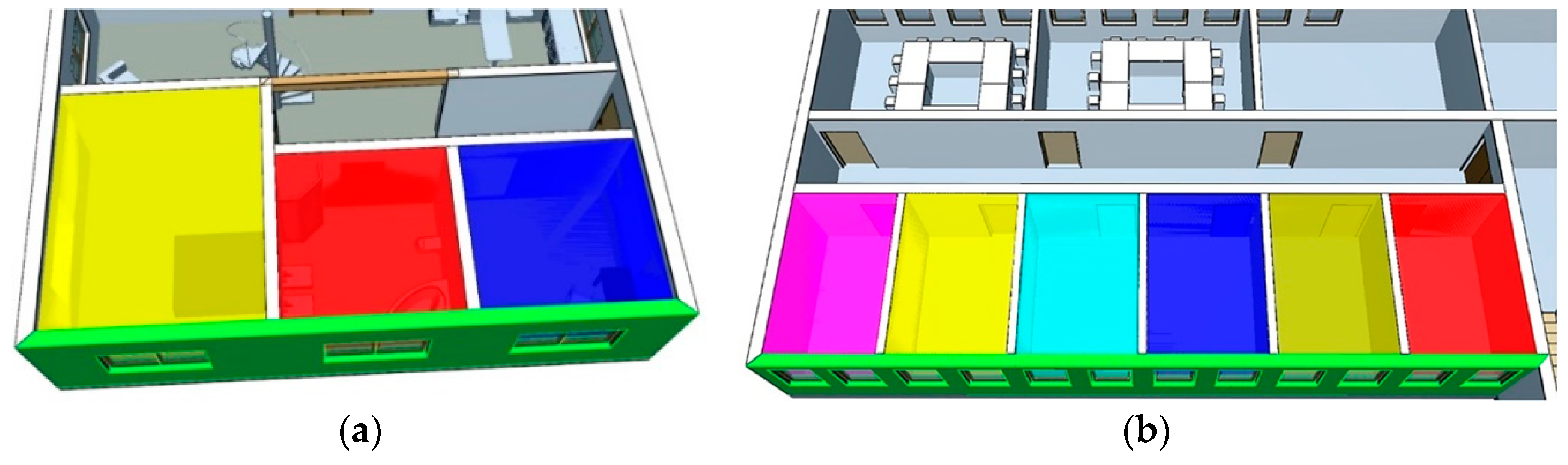
Most of the research done to date has mostly focused on two categories according to indoor GIS applications. The first category is CityGML modeling based on BIM models to visualization. Because CityGML models are commonly used in the field of GIS, this modeling method focuses on the conversion of data formats and realizes a model conversion by establishing correspondences between BIM and CityGML. However, this method inevitably loses the attribute information of BIM models, besides, the generating models (i.e., CityGML) lack indoor spatial features (such as adjacency relations) [8,9]. The second category is network modeling based on BIM models to support indoor navigation. Currently, existing commercial GIS platforms (such as ArcGIS) and open source libraries (such as IfcOpenShell and IFC++) support direct reading of BIM models, therefore, the category mainly focuses on the integration of indoor topological information (e.g., connectivity and geometric network model (GNM)) and BIM models according to IndoorGML. Concretely, the indoor GIS model mainly integrates path information generated from BIM connectivity relations and combines with the shortest path analysis algorithm to achieve GIS applications in indoor path planning and navigation [10,11,12,13,14]. However, the existing methods seldom regard the important adjacency in the IndoorGML standard, while the adjacency relations generally describe the location of cellular space (such as room 301, near room 201 on the second floor) [15,16,17]. Besides, the adjacent analysis is a critical spatial analysis of GIS that can realize the simulation analysis of indoor noise pollution and emergency response [18,19], therefore, in potential applications, when a fire breaks out in room 200, it is necessary to find cellular spaces affected by different adjacent degrees to decision service, but current research does not explore the relevant algorithm to meet the requirement. In addition, the current methods of extracting indoor adjacency cannot apply to the BIM model. For example, Lee and Kwan [18] proposed that if the polygons corresponding to two cellular spaces have a shared edge in the floor plan, they are adjacent, while the algorithm cannot be applied to the BIM model. Specifically, IfcSpace can acquire the adjacent wall information, but multiple IfcSpace objects can share one wall, which means it is not feasible that adjacency relations of the IfcSpace are obtained by the method of sharing the same wall (as shown in Figure 1). Therefore, there is currently no indoor adjacency extraction algorithm based on BIM Models.

In summary, current modeling methods based on BIM models mainly refer to CityGML or IndoorGML standards. However, current BIM models and methods lack important indoor adjacency relations and adjacent analysis. Therefore, the main problem in generating indoor GIS models based on BIM models is to integrate the spatial features (e.g., indoor adjacency relations) in the BIM model to support the adjacent analysis of indoor spaces. We herein developed a method for the generation of indoor GIS models based on BIM models to support adjacent analysis of indoor spaces. The method consists of three steps. First, we devised a new indoor GIS model with indoor adjacency relations, called IGSM, to support basic adjacent queries or analysis of indoor spaces. Second, considering the shortage of an indoor adjacency extraction algorithm from BIM models and the practicability of indoor GIS models, we devised an automated rapid modeling algorithm to transform a BIM model into an IGSM. Finally, we designed a K-adjacent analysis algorithm to improve adjacent analysis of indoor spaces.

2. Related Works

The existing methods for the generation of indoor GIS models based on BIM models can be divided into two categories according to application: (1) Methods for generating CityGML models based on BIM models. (2) Methods for generating indoor GIS model based on BIM models to navigation.

2.1. Methods for Generating CityGML Models Based on BIM Models

The CityGML model is a building model commonly used in the field of GIS and has indoor building information [20,21]. Some scholars have proposed the modeling method of transforming BIM models into CityGML models. De Laat and van Berlo extended the CityGML data type to transform BIM models into CityGML models [22,23]. However, CityGML models have different information on the levels of detail (LODs). Besides, as shown in Figure 2, CityGML models have different information on the levels of detail (LODs), which includes the five LODs (from LOD0 to LOD4). With the increase in LOD, the model has more geometric and semantic details. Accordingly, Deng et al. and Donkers et al. investigated the conversion relationship between BIM and different CityGML LODs and developed a more accurate automated modeling method for CityGML [6,24]. They realized the automated modeling of CityGML by simplifying BIM models, thereby promoting the application of BIM models in the field of GIS to some extent. However, some geometric and semantic information in the BIM model could be lost during the conversion process, and the model lacked information on indoor spatial features.

2.2. Methods for Generating Indoor GIS Models Based on BIM Models to Navigation

Three-dimensional GIS software and Industry Foundation Classes (IFC) open-source libraries support the parsing and reading functions of the IFC standard in the BIM model; hence, the indoor navigation modeling method based on BIM models builds 3D GIS models with indoor spatial features through GIS platforms or open-source libraries [14,26,27].

Table 1. Comparative analysis of indoor geographic information system (GIS) models.

Model.	Author	Spatial Features		3D GIS Platform	Spatial Analysis Ability
		Spatial Position	Topological Relation
BO-IDM	Umit Isikdag et al.	√	Connectivity	ArcGIS	Potential for indoor navigation
-	Azarakhsh et al.	√	Connectivity	-	Viewshed and shadow analysis
-	Chen et al.	√	GNM	-	Firefighting simulation
IESM	Tashakkori et al.	√	GNM	ArcGIS	Emergency navigation
MGNM	Teo and Cho	√	GNM	ArcGIS	Indoor and outdoor path planning

shows the statistics of relevant models in recent years, such as the BIM oriented indoor data model (BO-IDM), the indoor emergency spatial model (IESM), the multi-purpose geometric network model (MGNM) and so on. Note, “-” indicates not mentioned; the spatial position indicates whether the model has real geographic coordinates, and the topological relation is for cellular spaces.

Table 1 shows that the abovementioned modeling methods imported BIM models through the commercial 3D GIS platform ArcGIS to generate indoor 3D GIS models. ArcGIS used the Feature Manipulate Engine (FME) plug-in (spatial data conversion and processing system) to realize the expression of the geometric and semantic information of the BIM model and incorporated important feature information in the modeling process to form various indoor 3D GIS models [13,28]. The BO-IDM modeling method simplified the geometric and semantic information of the BIM model to retain the information needed for indoor navigation and realized the automated modeling of indoor 3D GIS models [8]. The IESM automated modeling method incorporated indoor path information and important firefighting equipment in the modeling process to realize decision-making and path analysis under the emergency response condition [19]. The MGNM modeling method considered the emergency path information from the room to the window and optimized the staircase path extraction method to realize automated modeling of the model, which could be used for indoor and outdoor path analysis [29]. The abovementioned modeling methods focused on the ability of the indoor path analysis and put forward various extraction algorithms for building indoor paths. The modeling processes preserved the connectivity of the cellular space in the BIM model, but overlooked the adjacency relations between cellular spaces, resulting in an eventual failure to realize the adjacent query and analysis of the cellular space.

In addition, Azarakhsh et al. proposed a method for generating indoor GIS models based on BIM models and realized the viewshed and shadow analysis function of BIM in GIS systems [5]. Chen et al. used OpenGL to build an indoor 3D GIS model applicable to firefighting simulation and elaborated on the 3D GNM generation algorithm [30]. Nevertheless, in the aforementioned modeling methods, the positional expression of the BIM model to the GIS system was not explicitly stated, and the adjacency relations of indoor cellular spaces were not considered, which limited the applicability of indoor GIS.

In summary, current indoor navigation modeling based on BIM models realize the automated modeling process of the model, and existing methods mainly focus on the indoor connectivity relations or path information. Nonetheless, such modeling methods overlooked important adjacency relations from IndoorGML and could not realize the adjacent query and analysis of indoor spaces when applied to the GIS system.

In this regard, the subsequent sections are arranged as follows: Section 3 discusses the methodology; Section 3.1. introduces the organizational form of the indoor 3D GIS data model (IGSM), which laid the foundation for indoor spatial analysis; Section 3.2. explains the IGSM modeling algorithm that examines how to generate the IGSM from the BIM model to realize the rapid modeling of indoor GIS models; Section 3.3. explains the K-adjacent analysis algorithm that introduces an extended adjacent analysis algorithm applicable to IGSM, thereby improving the adjacent analysis of indoor spaces for 3D GIS; Section 4 is the experimental step used to verify the effectiveness of the proposed method; Section 5 provides the conclusion of this study and the future work.

3. Methodology

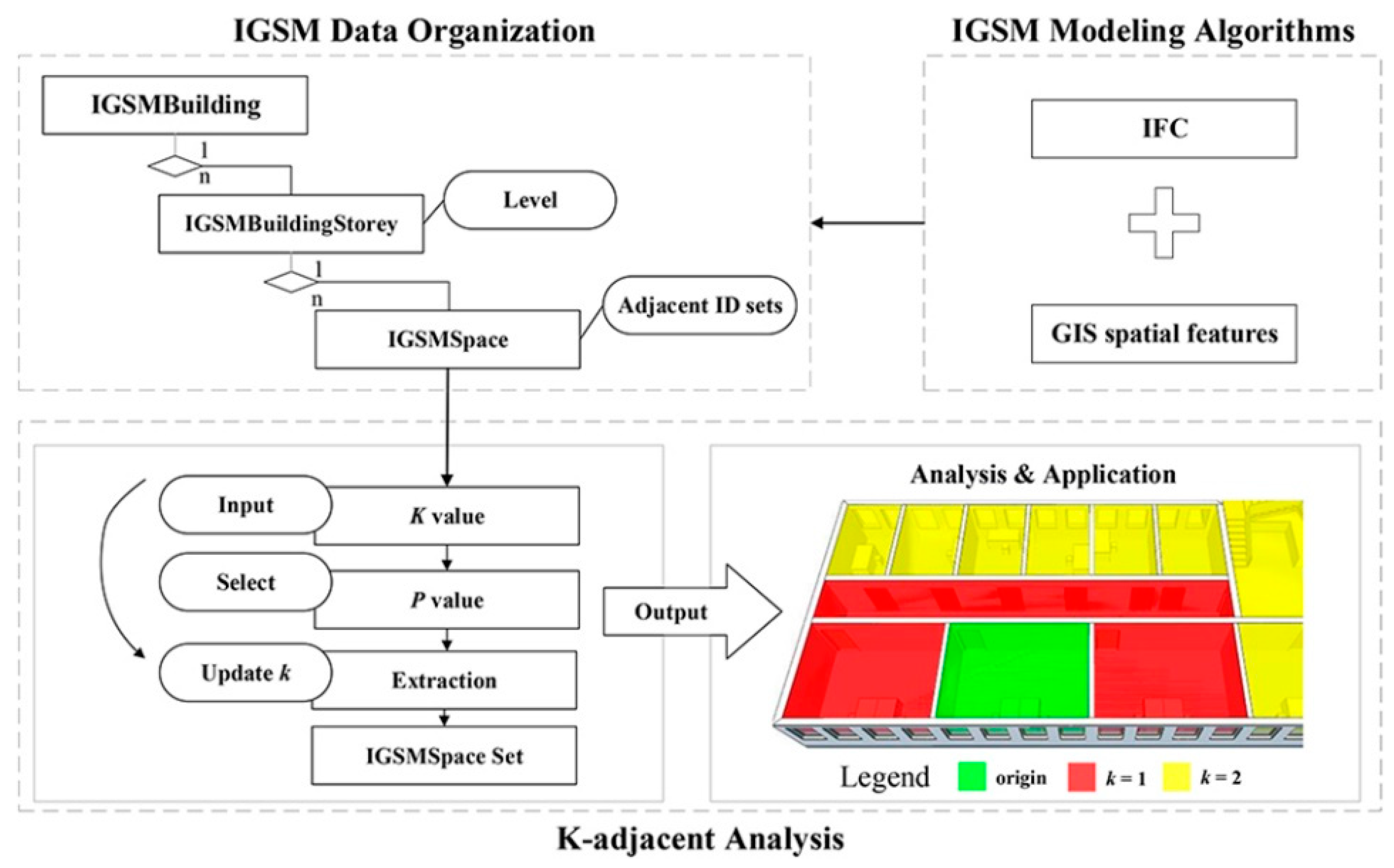
We devised a method for the generation of indoor GIS models based on BIM models. This method included three steps (as shown in Figure 3). First, we integrated the necessary spatial feature information (i.e., geometric location and topological relation) based on BIM models and proposed an indoor 3D GIS building model applicable to the adjacent analysis, called IGSM. Then, we proposed an IGSM modeling algorithm based on BIM models according to the organizational mode of IGSM and the feature of the BIM model. Finally, we proposed a K-adjacent analysis algorithm to improve the adjacent analysis of cellular spaces.

3.1. IGSM Data Organization

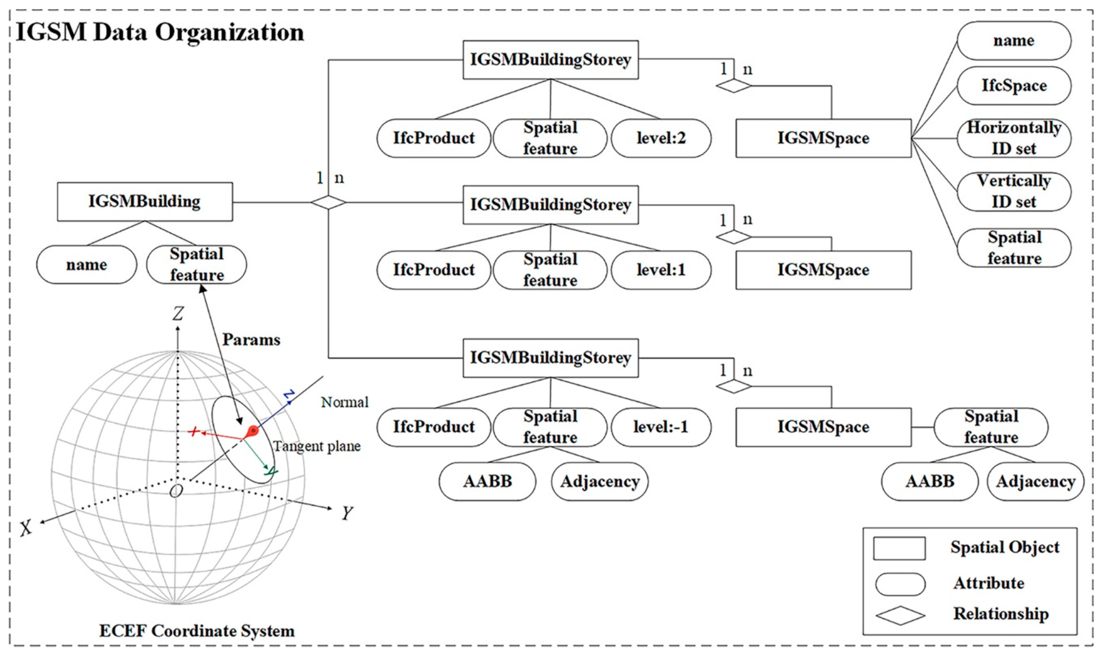
We developed an indoor 3D GIS building model (IGSM) to realize the basic adjacent query and analysis of the indoor GIS. Figure 4 shows that the IGSM was divided according to the three-tier spatial structure of conventional buildings, namely the IGSMBuilding, IGSMBuildingStorey, and IGSMSpace. In addition, the spatial structure of each tier incorporated spatial feature information.

3.1.1. IGSMBuilding

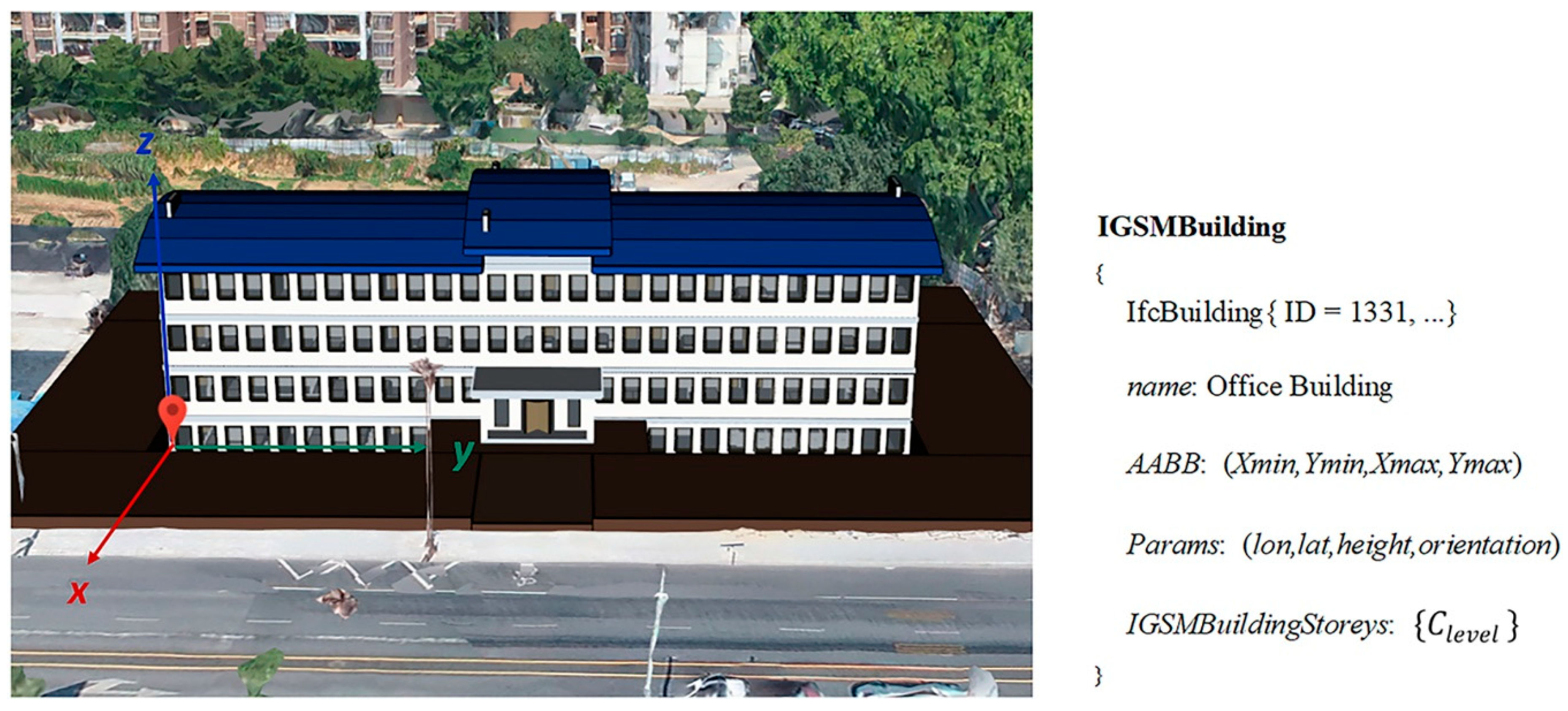
Figure 4 and Figure 5 show that IGSMBuilding was mainly used to describe the spatial feature information of the building as a whole based on IfcBuilding. Besides, the spatial structure recorded the information on the geometric location parameter of the current model, namely $Params$, including geographic parameters, such as longitude, latitude, height, and orientation, in the WGS84 coordinate system. The objective expression of the geometric location of the model was realized through Algorithm 1 in Section 3.2.1. Moreover, the IGSMBuilding contained the IGSMBuildingStorey set $\left\{C_{level}\right\}$.

3.1.2. IGSMBuildingStorey

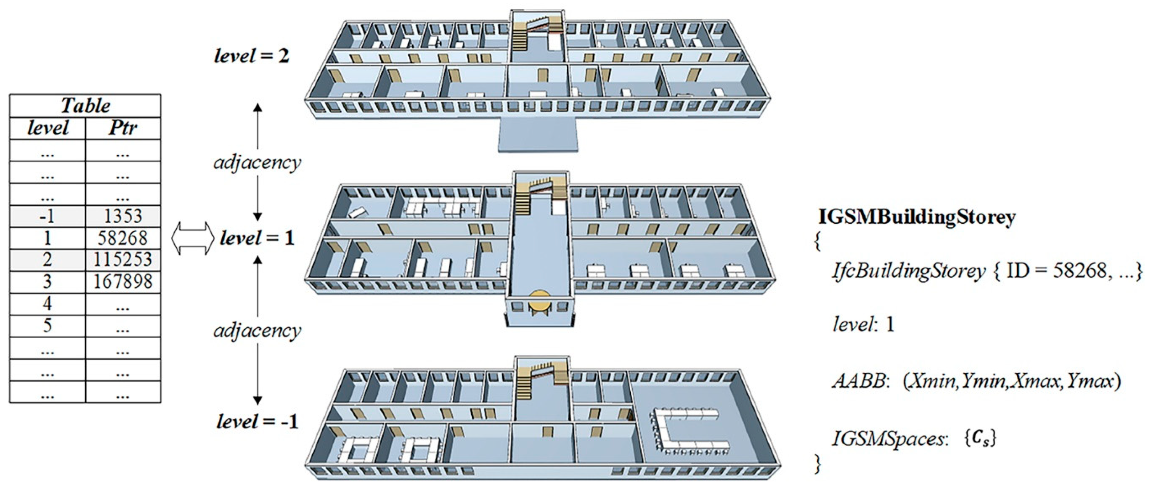
Figure 6 shows that the spatial structure IGSMBuildingStorey contained IGSMBuildingStorey and IfcProduct, which recorded the $level$ number and index table $T\left(level,C_{level}\right)$. $T$ was automatically sorted incrementally according to the $level$ value. $C_{level}$ stood for IGSMBuildingStorey. Figure 6 shows that the adjacency relations between the floors were realized through index table $T$. The $level$ of IGSMBuildingStorey obtained $level-1$ and $level+1$ through $T$, which corresponded to $C_{level-1}$ and $C_{level+1}$, respectively. In addition, IGSMBuildingStorey recorded the IGSMSpace set $\left\{C_s\right\}$.

3.1.3. IGSMSpace

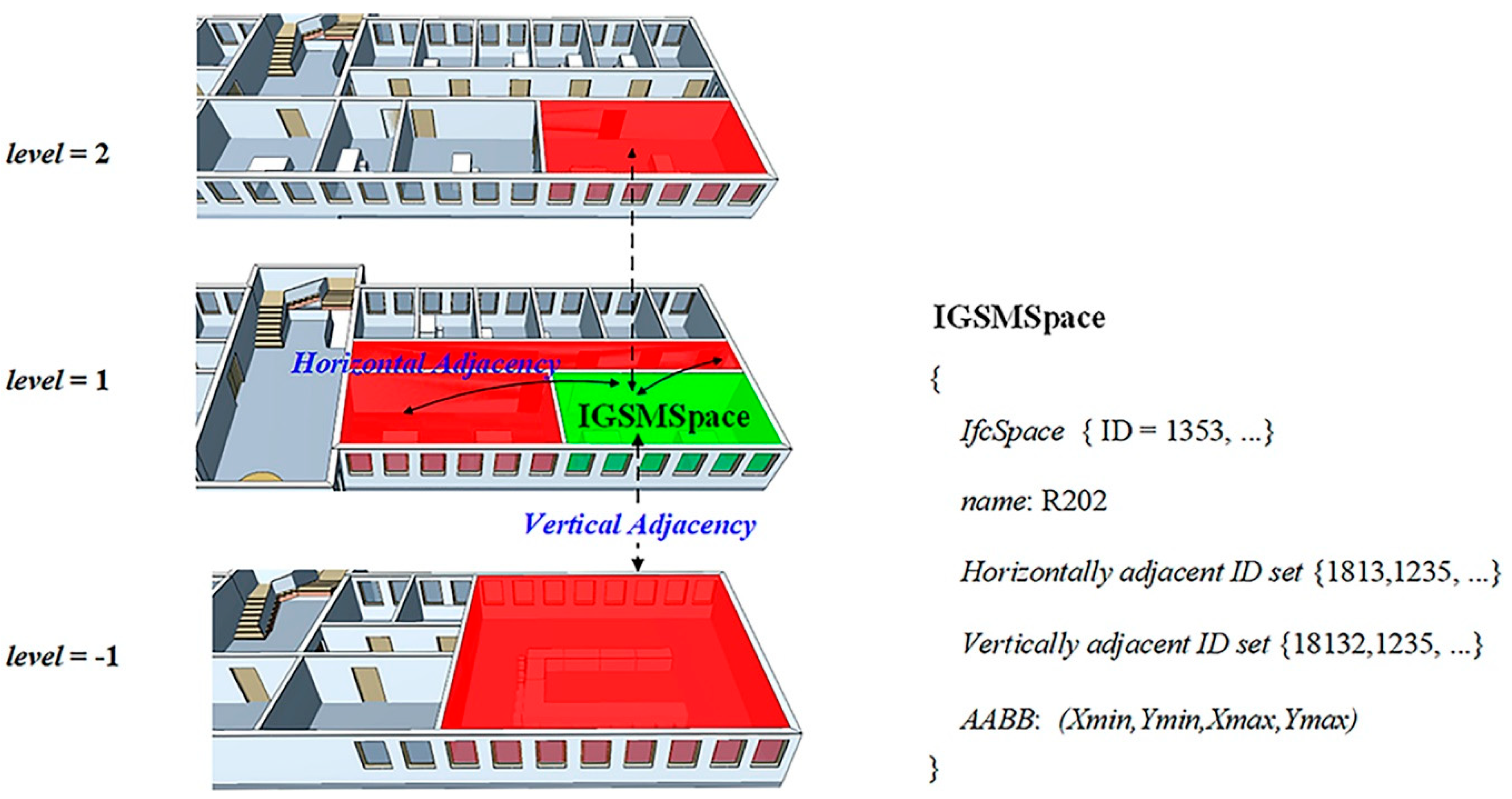
Figure 7 shows that the spatial structure IGSMSpace contained IfcSpace and recorded the adjacent ID sets, including the horizontally adjacent ID set $\left\{C_h\right\}$ and the vertically adjacent ID set $\left\{C_v\right\}$. The adjacency relation of $\mathrm{IGSMSpace}$ was realized through $\left\{C_h\right\}$ and $\left\{C_v\right\}$. The traversal set $\left\{C_h\right\}$ obtained the adjacent $\mathrm{IGSMSpace}$ on the same floor through the ID information. Similarly, the traversal set $\left\{C_v\right\}$ obtained the adjacent IGSMSpace on the same floor through the ID information.

3.2. IGSM Modeling Algorithms

Using the semantic and geometric features of the BIM (IFC format) models, we constructed modeling algorithms from BIM models to IGSMs, which were processed according to the spatial structure level of the BIM models: IfcBuilding, IfcBuildingStorey, and IfcSpace. Each spatial structure corresponded to an algorithm, and three algorithms were constructed for geographic location mapping, floor relation extraction, and indoor adjacency extraction. Among them, the geographic location mapping mainly described how to locate the geographic position of the BIM model on the GIS platform, which integrates the BIM model into the 3D GIS platform. The floor relation extraction mainly derived the floor number of the model, and defined the adjacent relationship between floors through the floor number. The indoor adjacency extraction acquired the indoor adjacency relations between cellular spaces, and mainly included adjacency of the same floor and adjacent floors. Figure 8 shows the overall flow chart of the IGSM modeling algorithms. The BIM element of each algorithm was the input data, whereas the IGSM element was the output data.

3.2.1. Geographic Location Mapping

The BIM model mainly builds the Cartesian coordinate system based on (0,0,0) of IfcSite (i.e., local coordinate system), while the 3D GIS model generally adapts the coordinate system of Earth Center Earth Fixed (ECEF) in the GIS environment (such as a virtual globe) [5,31,32,33]. Considering that IfcSite defines an area where construction works, which optionally stores the geographic location using the RefLatitude, RefLongitude, and RefElevation is attributed to the World Geodetic System published in 1984 (WGS84), the current methods mainly link the local coordinates of a BIM model with their corresponding geographic coordinates in the GIS environment [5,9,32]. Besides this, some scholars realized the georeferencing of BIM in the projection coordinate system. However, it is necessary to minimize scale distortions caused by projection transformation (importing scale factors) because distortions in a map projection can be amplified for large-scale longitudinal projects (e.g., roads and railroads) [31,33]. Therefore, considering that buildings are small-scale projects, and the relative accuracy of the model is high, we directly link the BIM model coordinate system into the ECEF coordinate system in the GIS environment, which avoids the projection transformation distortions (ignoring scale distortions). The proposed algorithm detailed illustrated a mapping process according to the parameter $Params$ of the IGSM (see Section 3.1), which laid the basis of spatial analysis and applications of the BIM model in 3D GIS. The detailed description can be shown in Algorithm 1.

Algorithm 1. Geographic Location Mapping Algorithm
1:	Input:
2:	(1) The BIM model; (2) the parameter $Param$.
3:	Output:
4:	(1) IGSMBuilding.
5:	Initialize:
6:	(1) Parse the local coordinates $\left\{\left(x,y,z\right)\right\}$ inside the BIM model by an IFC parser
7:	Step1. Positioning: obtain $LocationMatrix$.
8:	Step2. Alignment: obtain $RotateZMatrix.$
9:	Obtain $TransformMatrix$ by Formula (4).
10:	for each coordinate $\left(x,y,z\right)$ in $\left\{\left(x,y,z\right)\right\}$
11:  12:	$\left[\begin{array}{c}X\\ Y\\ Z\end{array}\right]=TransformMatrix\left[\begin{array}{c}x\\ y\\ z\end{array}\right]$
13:	end for
14:	return IGSMBuilding.

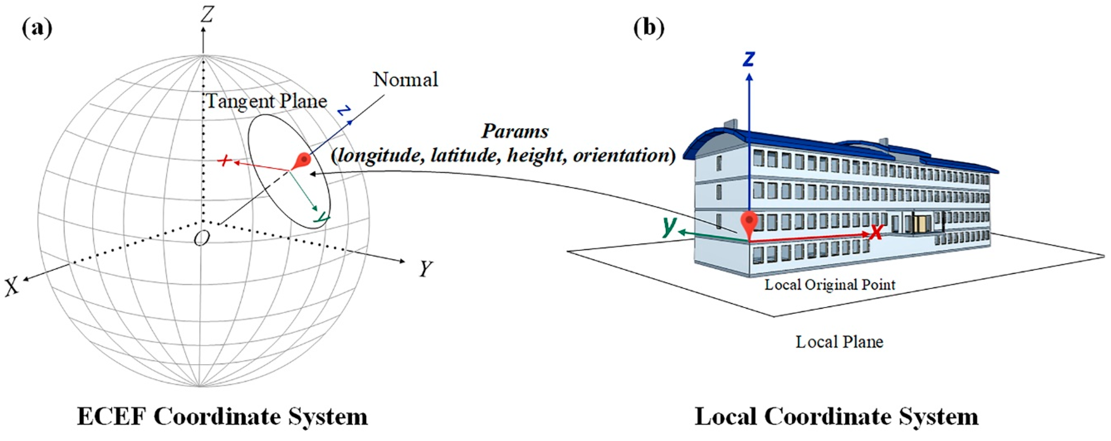
For illustration purposes, two spatial objects, namely Tangent Plane and Local Plane, were defined in this study. Figure 9a shows that Tangent Plane is the tangent plane of the corresponding point of the BIM model on the earth, corresponding to the local scene of the 3D GIS, and its normal vector coincided with the normal vector of the earth ellipsoid Normal. Local Plane is the coordinate system o-xy plane defined by IfcBuilding in BIM as shown in Figure 9b. Note that the current GIS platform (such as a virtual globe) mainly adapts the geographic coordinate system WGS84. Moreover, the WGS84 can easily convert to another coordinate system. Therefore, the parameter $Params$ in the algorithm stores the location information of the WGS84.

Step 1. Positioning: The Local Plane of $\mathrm{IfcBuilding}$ coincided with the Tangent Plane of the 3D GIS. At this time, the coordinate axis Z, where the IfcBuilding of the BIM model was located, coincided with the normal vector of the Tangent Plane. Considering the WGS84 ellipsoid as an example (semi-major axis $a$, semi-minor axis $b$), we obtained the $LocationMatrix$ using the longitude ($lon$), latitude ($lat$), and height ($h$), transforming all geometric information on the BIM model, to realize the positioning process of the model. The specific conversion matrix is presented below

$$LocationMatrix=\left[\begin{array}{cc}\begin{array}{cc}EastX& NorthX\\ EastY& NorthY\end{array}& \begin{array}{cc}UpX& X\\ UpY& Y\end{array}\\ \begin{array}{cc}EastZ& NorthZ\\ 0& 0\end{array}& \begin{array}{cc}UpZ& Z\\ 0& 1\end{array}\end{array}\right],$$

(1)

where vector $\stackrel{\rightharpoonup }{East}=\left(EastX,EastY,EastZ\right)=\left(-\sin \left(lon\right),\cos \left(lon\right),0\right)$; vector $\stackrel{\rightharpoonup }{Up}=\left(UpX,UpY,UpZ\right)=\left(\cos \left(lon\right)\times \cos (lat),\sin (lon)\times \cos (lat),\sin \left(lat\right)\right)$; and vector $\stackrel{\rightharpoonup }{North}=\left(NorthX,NorthY,NorthZ\right)=\stackrel{\rightharpoonup }{Up}\times \stackrel{\rightharpoonup }{East}$.

X, Y, and Z accordingly converted the longitude, latitude, and height of the ellipsoid into the corresponding coordinates of ECEF expressed by Formula (2) as follows [31]

$$\left[\begin{array}{c}X\\ Y\\ Z\end{array}\right]=\left[\begin{array}{c}\left(N+h\right)\times cos(lat)\times cos(lon)\\ \left(N+h\right)\times cos(lat)\times sin(lon)\\ (\left(N\times \left(1-e^2\right)+h\right)\times sin\left(lat\right)\end{array}\right],$$

(2)

where $N=a/\sqrt{(1-{\left(e\times \sin (lat)\right)}^2}$ was the mean curvature radius at the given latitude $lat$, $e=\raisebox{1ex}{$\sqrt{a^2-b^2}$}\!\left/ \!\raisebox{-1ex}{$a$}\right.$ was the first eccentricity [31].

Step 2. Alignment: The correct orientation of the BIM model on the GIS platform was achieved by rotating θ around the Z-axis of the model. The rotation matrix $RotateZMatrix$ could be expressed as

$$RotateZMatrix=\left[\begin{array}{cccc}1& 0& 0& 0\\ 0& cos\theta & sin\theta & 0\\ 0& -sin\theta & cos\theta & 0\\ 0& 0& 0& 1\end{array}\right],$$

(3)

Therefore, the final transformation matrix $TransformMatrix$ was formed according to the two processes of positioning and alignment.

$$TransformMatrix=RotateZMatrix\times LocationMatrix,$$

(4)

In summary, we obtained the transformation matrix $TransformMatrix$ by calculating through Formula (4) and performing the matrix transformation of each vertex coordinate in the model to realize the transformation from $\mathrm{IfcBuilding}$ to IGSMBuilding. Besides this, the practical application can be divided into two strategies according to the entire lifecycle of a project: (1) For the plan or design stage of the project, the parameter $Params$ can be obtained through IfcSite and IfcProject of the BIM mode l [5,9,32]. When the model is loaded into the GIS platform through the geographic location mapping algorithm, the geometric position of the model on the GIS platform is modified by adjusting the parameter $Params$ interactively. (2) For the operation or maintenance stage of the BIM model, we can first obtain geographic information (longitude, latitude, and elevation) of the origin of IfcSite through the Real-Time Kinematic (RTK) and other equipment. Then, the alignment with the actual building can be obtained through the matrix. In this time, another exterior corner of the BIM model can be selected to obtain the corresponding position information through location equipment, and the angle between vectors can be calculated to get the rotation matrix combining the origin of IfcSite. Meanwhile, several coordinate points for the BIM model in the GIS environment and the reference points of the actual building are selected to realize the accuracy evaluation (such as Root Mean Square Error).

3.2.2. Floor Relation Extraction

The floor relation extraction algorithm mainly derived the floor number of each floor in the model, indicating the relative location between stories, which was also the necessary premise of the indoor topology extraction algorithm. Considering that the attribute of Elevation in each IfcBuildingStorey of the BIM model stored the elevation value relative to the building, the algorithm sorted these values and gives the floor number, which established the adjacency relations. Finally, each IGSMBuildingStorey saved relevant attributes, Section 3.1 IGSM data organization explained its specific storage method. Algorithm 2 shows its detailed description.

Algorithm 2. Floor Relation Extraction Algorithm
1:	Input:
2:	(1) IfcBuildingStorey set $\left\{S\right\}$; (2) Unit conversion factor of the BIM model $Factor$.
3:	Output:
4:	(1) IGSMBuildingStorey set with $level$ number, i.e., $\left\{C_{level}\right\}$; (2) $level$ and index table
5:	of IGSMBuildingStorey $T\left(level,C_{level}\right)$.
6:	Initialize:
7:	(1) Set $C$ and $T$ to $NULL$; (2)$threshold=0.5$; (3) Set index tables $T_p\left(height,S\right)$ and
8:	$T_m\left(height,S\right)$ to $NULL$. Sorted $T_p$ in increasing order of $height$ and $T_m$ in decreasing
9:	order of $height$. $T_p$ and $T_m$ included elevation $height$ and BIM level information $S$.
10:	for each$c$ in $C$.
11:	Got the Elevation field value $Value$ and ID value $id$ of $c$; set $Z=Value\times Factor$.
12:	if $Z\ge 0 or \left(threshold+Z\right)\ge 0$
13:	Insert $Z$ and IfcBuildingStorey $c$ into $T_p$; insert $Z$ and $id$ into $T$.
14:	else
15:	Insert $Z$ and IfcBuildingStorey $c$ into $T_m$; insert $Z$ and $id$ into $T$
16:	end if
17:	end for
18:	Set $level=1$.
19:	for each$t$ in $T_p$
20:	Insert $S$ and $level$ in $t$ into $C$, $level=level+1$.
21:	end for
22:	Set $level=-1$.
23:	for each$t$ in $T_m$
24:	Insert $S$ and $level$ in $t$ into $C$, $level=level-1$.
25:	end for
26:	return$C$ and $T$.
27:

The conversion factor $Factor$ in the algorithm was parsed from the IFC data format. However, $threshold$ assumed that the first floor was lower than the foundation to avoid classifying the first floor as the first basement floor, which enhanced the robustness of the algorithm.

3.2.3. Indoor Adjacency Extraction

The indoor adjacency extraction algorithm (Algorithm 3) mainly obtained the adjacent cellular spaces of each cellular space in the model, indicating the adjacency relations of indoor spaces. The algorithm converts the 3D model into images to achieve adjacency relations extraction, which can include the following four steps: 1. Indexing and rendering: each cellular space was assigned to a unique color value according to ID of the IfcSpace, and obtained the index table of color and ID. Then, the index table of color and ID could be obtained. The BIM model can be rendered using OpenGL technology according to the assigned colors (building elements of non IfcSpace were rendered in the same color blue); 2. Mapping and rasterization: each floor of the BIM model was converted into the rasterized floor plan. The relative location between the floor plans remained unchanged; 3. Vertical search: traversed the color value of the adjacent rasterized floor plan to obtain the adjacent cellular spaces between adjacent floors according to the above index table; 4. Horizontal search: for each rasterized floor plan, the color value was traversed along the boundary (e.g., wall) to obtain the adjacent cellular spaces of each space according to the above index table. The specific algorithm can be described as follows

Algorithm 3. Indoor Adjacency Extraction Algorithm
1:	Input:
2:	IfcSpace set inside the IGSMBuildingStorey set with level number $\left\{C_{level}\right\}$.
3:	Output:
4:	IGSMSpace set inside the IGSMBuildingStorey.
5:	Initialize:
6:	Set index table of IfcSpace $T\left(id,color\right)$ to $NULL$.
7:	Step1. Indexing and rendering.
8:	Step2. Mapping and rasterization.
9:	Step3. Vertical search.
10:	Step4. Horizontal search.
11:	return IGSMSpace set inside the IGSMBuildingStorey.

Step 1. Indexing and rendering: The spatial structure IfcSpace in the BIM model has a unique ID value. The associated IfcSpace information could be uniquely identified by color by establishing the relationship between the ID value and the color mapping. Then, the index table of color and ID can be obtained. Finally, the BIM model can be rendered using OpenGL technology according to the assigned colors (building elements of non IfcSpace were rendered in the same color: blue). The detailed description can be shown in Algorithm 4.

Algorithm 4. Indexing and Rendering
1:	Input:
2:	The IfcSpace set inside the IGSMBuildingStorey set with level number $\left\{C_{level}\right\}.$
3:	Output:
4:	The index table of IfcSpace $T\left(id,color\right)$; the rendered IGSMBuildingStorey set $\left\{C_{level}^{\prime }\right\}.$
5:	Initialize:
6:	Set $T$ = $NULL$.
7:	for each$c$ in $\left\{C_{level}\right\}$
8:	for each building element $b$ in $c$
9:	Set $value=NULL$.
10:	if $b=$ IfcSpace
11:	Insert a unique color $value=$ (R, G, B, 0.8) and ID of IfcSpace into $T$.
12:	else
13:	Set $value=\left(0, 0, 1, 1\right)$.
14:	end if
15:	Rendering $b$ in $value$ using fragment shader of GPU.
16:	end for
17:	end for
18:	return$T$ and $\left\{C_{level}^{\prime }\right\}$.

The color rendering of the BIM architectural elements used the fragment shader of GPU with the following pseudocode:

“ void main(void)\n”

“{\n”

“ gl_FragColor = vec4( #Red, #Green, #Blub, #Alpha);\n”

“}\n”

#Red, #Green, and #Blue specifically represent the color value corresponding to the ID value of IfcSpace (RGB mode), while #Alpha represents transparency, with both values ranging from 0.0 to 1.0.

Step 2. Mapping and rasterization: The IGSMBuildingStorey set $\left\{C_{level}^{\prime }\right\}$ in the building is converted into the rasterized floor plan set $\left\{I_{level}\right\}$. Among them, mapping converts each IGSMBuildingStorey into the floor plan through orthographic projection, whereas rasterization converts the plan into the corresponding texture (i.e., rasterized floor plan). The detailed description can be shown in Algorithm 5.

Algorithm 5. Mapping and Rasterization
1:	Input:
2:	The rendered IGSMBuildingStorey set $\left\{C_{level}^{\prime }\right\}$.
3:	Output:
4:	The rasterized floor plan set $\left\{I_{level}\right\}$.
5:	Initialize:
6:	Set $\left\{I_{level}\right\}$ to be $NULL$.
7:	for each$c_{level}^{\prime }$ in $\left\{C_{level}^{\prime }\right\}$.
8:	Step 3.2.1. Mapping.
9:	Step 3.2.2. Rasterization.
10:	end for
11:	return$\left\{I_{level}\right\}$.

Step 3.2.1. Mapping: Through the matrix change, each floor $C_{level}^{\prime }$ is converted into the floor plan by Z-axis orthographic projection as shown in Figure 9b, where the projection matrix is as follows

$$ProjectMatrix=\left[\begin{array}{cccc}1& 0& 0& 0\\ 0& 1& 0& 0\\ 0& 0& 0& 0\\ 0& 0& 0& 1\end{array}\right],$$

(5)

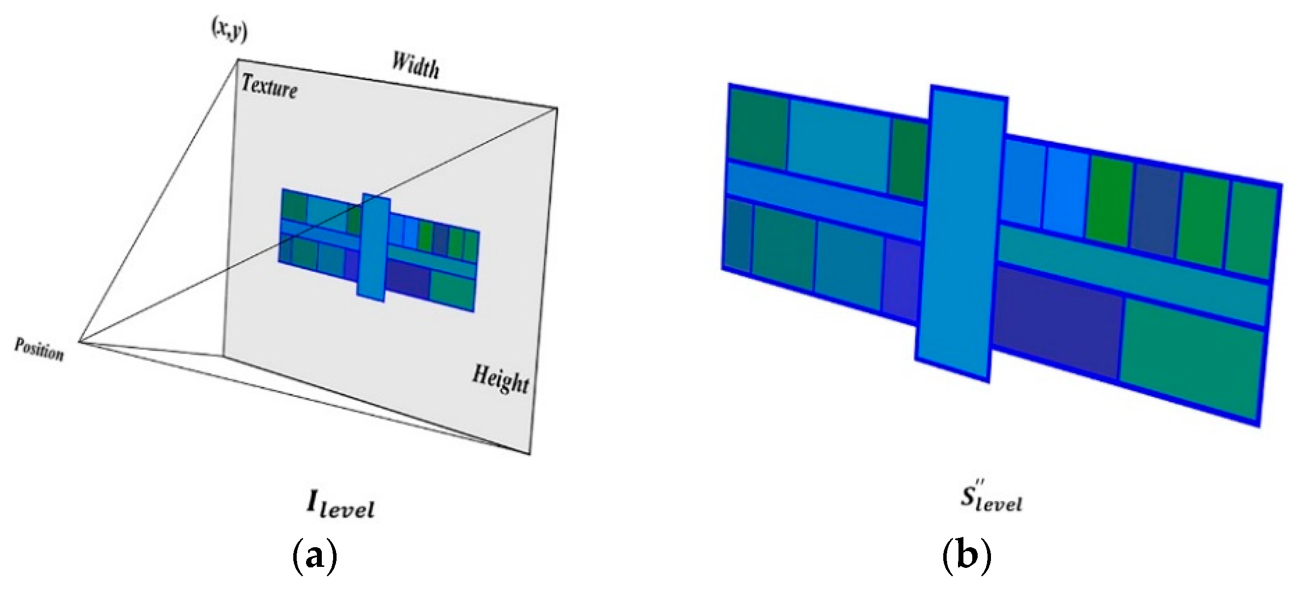
Step 3.2.2. Rasterization: As shown in Figure 10a, by traversing the rasterized floor plan set in Step 1, the Render To Texture technology (RTT) is used to save the frame generated by drawing in the form of a texture, which eventually forms the rasterized floor plan set $\left\{I_{level}\right\}$. Besides, rasterization requires consistent parameter setting information to ensure that the relative location of the cellular spaces between the levels remains unchanged.

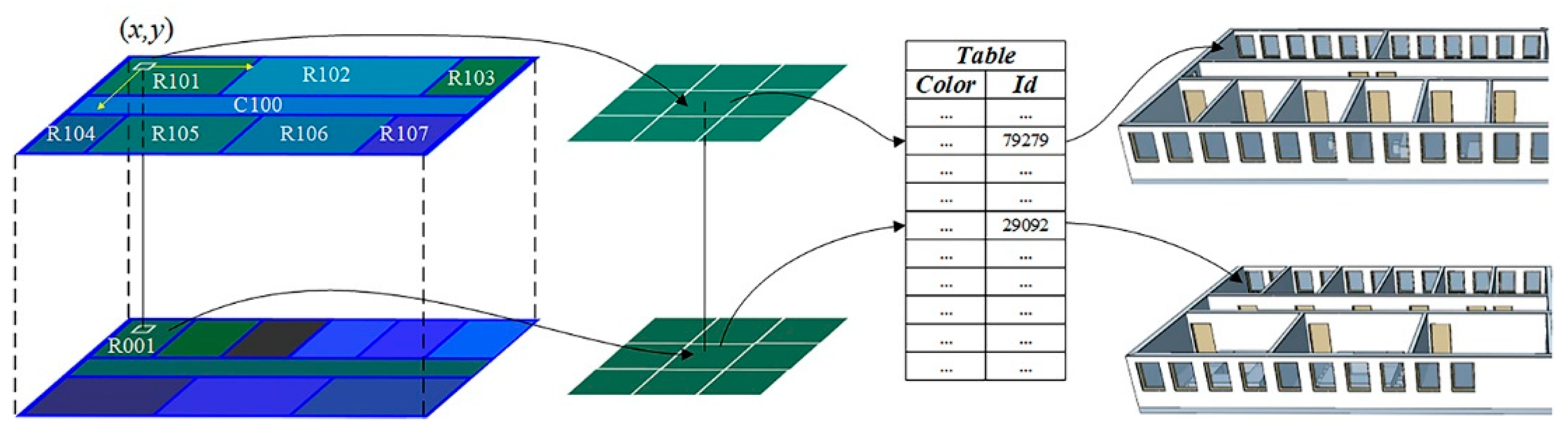
Step3. Vertical search: Traverse each pixel $\left(x,y\right)$ of the adjacent rasterized floor plan from $\left\{I_{level}\right\}$ obtains the corresponding color values. Then, according to the index table in Step 1, we can derive the adjacency relations of each cellular space in the vertical direction (Figure 11). The detailed description is shown in Algorithm 6.

Algorithm 6. Vertical Search
1:	Input:
2:	(1) The IfcSpace set inside the IGSMBuildingStorey set with level number $\left\{C_{level}\right\}$; (2)
3:	The rasterized floor plan set $\left\{I_{level}\right\}$; (3) The index table of IfcSpace $T\left(id,color\right).$
4:	Output:
5:	The IGSMSpace set with the vertically adjacent ID set.
6:	Initialize:
7:	Set $i=0$.
8:	Set index table of adjacency relations $T\left(id,\left\{id\right\}\right).$
9:	while$i<$ the number of $\left\{I_{level}\right\}$ − 1
10:	if $I_{level}\left(i\right)=0$ or $I_{level}(i+1)=0$
11:	return $NULL$.
12:	end if
13:	for each pixel value $Colo{r}_i\left(x,y\right)$ in $I_{level}\left(i\right)$ and $Colo{r}_{i+1}\left(x,y\right)$ in $I_{level}\left(i+1\right)$
14:	Obtain $I{d}_i\left(x,y\right)$ and $I{d}_{i+1}\left(x,y\right)$ by the index table $T\left(id,color\right)$.
15:	Insert $I{d}_{i+1}\left(x,y\right)$ into the ID set $\left\{id\right\}$ of $I{d}_i\left(x,y\right)$ by $T\left(id,\left\{id\right\}\right).$
16:	Insert $I{d}_i\left(x,y\right)$ into the ID set $\left\{id\right\}$ of $I{d}_{i+1}\left(x,y\right)$ by $T\left(id,\left\{id\right\}\right).$
17:	end for
18:	end while
19:	for each$id,\left\{id\right\}$ in $T\left(id,\left\{id\right\}\right)$
20:	The IGSMSpace corresponding $id$ insert $\left\{id\right\}$ in the vertically adjacent set.
21:	end for
22:	return The IGSMSpace set with the vertically adjacent ID set.

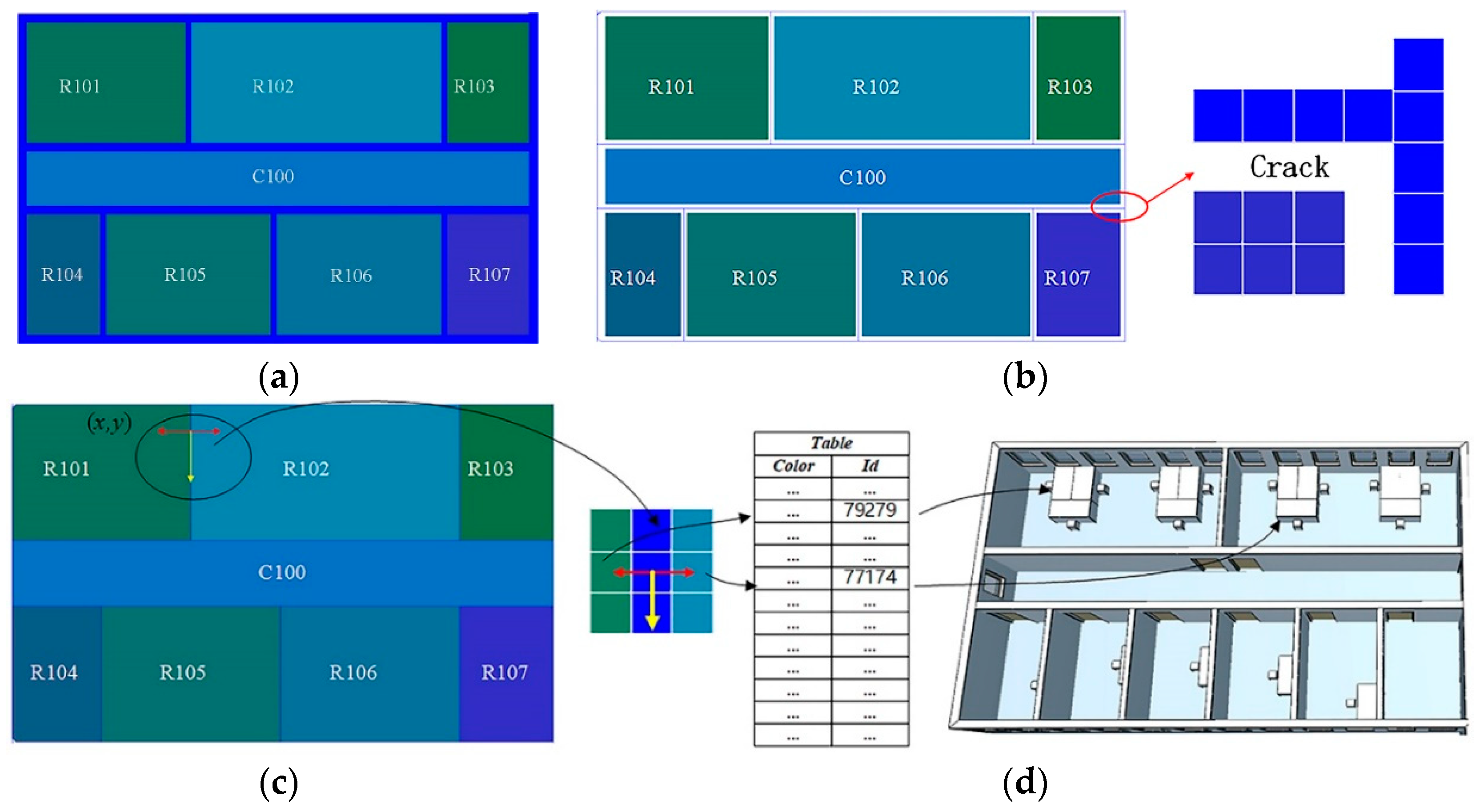
Step 4. Horizontal search: The adjacent IfcSpace on the same floor will share the “boundary” composed of walls or columns, and the “boundary” characterize continuous pixel set with line width greater than 1 for the rasterized floor plan. The blue part of the image in Figure 12a represents the “boundary” information of the model. Thus, when traversed along the “boundary” pixels and once adjacent color values are obtained for each rasterized floor plan, we can derive the adjacency relations of each cellular space in the horizontal direction through the above index table. The detailed description is shown in Algorithm 7.

Algorithm 7. Horizontal Search
1:	Input:
2:	(1) The IfcSpace set inside the IGSMBuildingStorey set with level number $\left\{C_{level}\right\}$; (2).
3:	The rasterized floor plan set $\left\{I_{level}\right\}$; (3) The index table of IfcSpace $T\left(id,color\right).$
4:	Output:
5:	The IGSMSpace set with the horizontally adjacent ID set.
6:	Initialize:
7:	Set index table of adjacency relations $T\left(id,\left\{id\right\}\right)$ to be $NULL$.
8:	for each$I_{level}$ in $\left\{I_{level}\right\}$
9:	if $I_{level}=0$
10:	return $NULL$.
11:	end if
12:	Step 3.4.1. Refinement and filling: obtain the image $I_{level}^{″}\left(i\right)$.
13:	Set $T\left(id,\left\{id\right\}\right)$ to be $NULL$.
14:	for each pixel value $Colo{r}_i\left(x,y\right)$ along the “boundaries” in $I_{level}^{″}\left(i\right)$ (Figure 12c)
15:	Obtain the adjacent color values $Colo{r}_1\left(x,y\right)$ and $Colo{r}_2\left(x,y\right)$ by the index table
16:	$T\left(id,color\right)$ (Figure 12d).
17:	Obtain $I{d}_1\left(x,y\right)$ and $I{d}_2\left(x,y\right)$ by the index table $T\left(id,color\right)$.
18:	Insert $I{d}_1\left(x,y\right)$ into the ID set $\left\{id\right\}$ of $I{d}_2\left(x,y\right)$ by $T\left(id,\left\{id\right\}\right).$
19:	Insert $I{d}_2\left(x,y\right)$ into the ID set $\left\{id\right\}$ of $I{d}_1\left(x,y\right)$ by $T\left(id,\left\{id\right\}\right).$
20:	end for
21:	end for
22:	for each$id,\left\{id\right\}$ in $T\left(id,\left\{id\right\}\right)$
23:	The IGSMSpace corresponding $id$ insert $\left\{id\right\}$ in the horizontally adjacent set.
24:	end for
26:	return The IGSMSpace set with the horizontally adjacent ID set.

Step 3.4.1. Refinement and filling: refine the blue “boundary” of the image $I_{level}\left(i\right)$ $(alpha$ = 0.8) to a linewidth equal to 1 px, thereby getting the image $I_{level}^{\prime }\left(i\right)$, as shown in Figure 12b. Fill the refined gap with the surrounding IfcSpace colors to form $I_{level}^{″}\left(i\right)$, as shown in Figure 12c. The refinement process adopts the classical refinement algorithm proposed by Zhang, which can be found in the literature [34].

Consequently, IGSM applicable to the adjacent query and analysis in 3D GIS was eventually formed through the abovementioned modeling algorithm by converting a BIM model to an IGSM.

3.3. K-Adjacent Analysis Algorithm for the IGSM

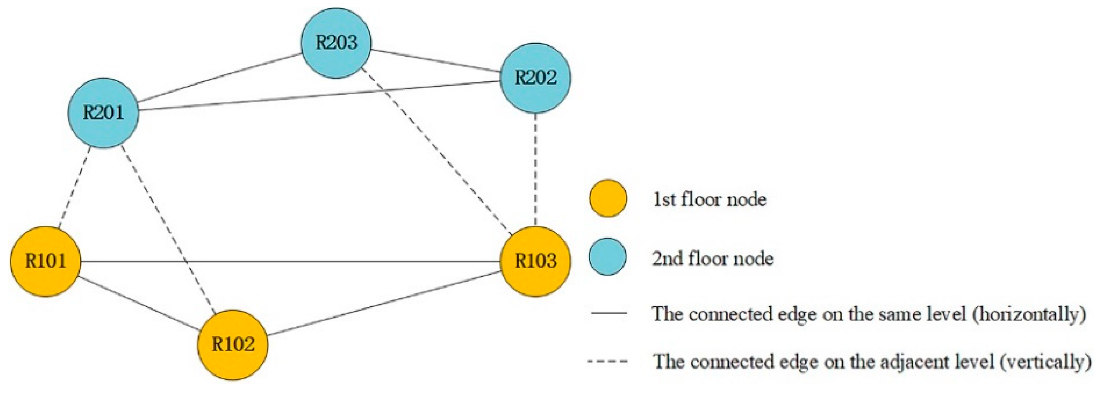
The IGSM or similar model can achieve basic adjacent query and analysis. However, in potential emergency response, the model hardly finds cellular spaces affected by different adjacent degrees to decision service. Therefore, we developed an adjacent analysis algorithm of indoor spaces, called the K-adjacent analysis algorithm for the IGSM (Algorithm 8). We first explain the relevant concepts. In Figure 13, the adjacency relations between the cellular spaces are represented by graph $G\left(V,E\right)$. In the graph, the cellular space is abstracted as node $V$. The adjacency relations between the nodes are represented by the edge $E$, and the length of the edge $D$ is set to 1. In this study, the adjacency degree of the indoor cellular spaces $K$ is defined as the minimum distance $D_{min}$ from the starting cellular space to the target cellular space. Accordingly, $D_{min}=1$ indicates that the starting space is adjacent to the target space, such as R202 and R203. Note that the edge $E$ falls into two categories: the connected edge of the cellular spaces on the same level (horizontally) and the connected edge of the cellular spaces on adjacent levels (vertically).

According to the earlier discussion, by specifying the starting cellular space, the K-adjacent analysis algorithm calculated a set of target cellular spaces, whose surrounding adjacency degree was not greater than K, to improve the applications of the adjacent analysis. The K-adjacent Algorithm can be detailed described as follows.

Algorithm 8. K-adjacent Algorithm
1:	Input:
2:	((1) Arbitrary IGSMSpace $S$; (2) Adjacency degree $K \left(K\ge 1\right)$; (3) Adjacency category $P$.
3:	$(P=1 \mathrm{denoted} \mathrm{horizontal} \mathrm{direction}; P=2 \mathrm{denoted} \mathrm{vertical} \mathrm{direction};\mathrm{and} P=$ 3 denoted
4:	arbitrary direction.
5:	Output:
6:	The index table of IGSMSpace $T\left(K,C\right)$, in which $C=\left\{c\right\}$ and $C$ denotes the ID set.
7:	Initialize:
8:	(1) $T\left(K,C\right)$ = NULL; (2) the global ID set $\left\{C_g\right\}$ was set to NULL; (3) $k=1$.
9:	while$k\le K$
10:	Set the temporary ID set $\left\{C_t\right\}$ to NULL.
11:	if $P=1$
12:	Obtain the horizontally adjacent ID set in $S$ $\left\{C_h\right\}$ and store it in $\left\{C_t\right\}$.
13:	else if $P=2$
14:	Obtain the vertically adjacent ID set in $S$ $\left\{C_v\right\}$ and store it in $\left\{C_t\right\}$.
15:	else
16:	Obtain $\left\{C_h\right\}$ and $\left\{C_v\right\}$ in $S$ and store them in $\left\{C_t\right\}$.
17:	end if
18:	Remove duplicate ID values in $\left\{C_t\right\}$ that are the same as those in $\left\{C_g\right\}$.
19:	if $\left\{C_t\right\}=0$
20:	return $T\left(K,C\right)$.
21:	else
22:	Store $\left\{C_t\right\}$ to $Se{t}_e$ and the current $k$ and $\left\{C_t\right\}$ to $T\left(K,C\right)$.
23:	end if
24:	$k=k+1$.
25:	end while
26:	return$T\left(K,C\right)$.

The ID value of the cellular spaces with different adjacency degrees (K) could be obtained through the K-adjacent analysis algorithm. The ID information could be used to quickly obtain the corresponding cellular space information for subsequent applications such as related analyses.

Therefore, as shown in Section 3.1, the three tiers constituted the IGSM defined in this study. IGSM adopted the geometric and semantic information defined by the BIM building element (IfcProduct) and incorporated the spatial feature information, which could be used for the adjacent query and analysis of cellular spaces and subsequent applications, such as indoor path planning. Specifically, the object of IGSMBuilding describes the geo-characteristics of the model in an outdoor environment to realize outdoor analysis and applications of building models, such as visualization and shadow analysis. The floors and the cellular spaces of the IGSMBuilding reflected the indoor spatial structure in a coarse-to-fine manner. The adjacent analysis of indoor spaces was conducted in combination with the proposed K-adjacent analysis algorithm, which enhanced the spatial analysis ability of the indoor 3D GIS.

4. Results

We verified the validity of the proposed method using the BIM model parsing library IFC++ and open-source virtual globe platform osgEarth to perform the relevant experiments [35,36]. The software environment was Windows 10 64-bit, OpenGL, and Microsoft Visual Studio 2015, while the hardware environment was Intel (R) Core (TM) i7-8750H CPU and NVIDIA GeForce GTX 1060 graphics card. The experimental data were selected from the following three typical building models processed by Revit software and exported to the IFC data format.

Table 2. Experimental data.

Name	IFC Version	Entity Number	Number of Floors	Thumbnail Image
FZK Haus	IFC4	14268	2
Office Building	IFC4	147712	5
Office Building2	IFC4	9169	3

presents a detailed description of the experimental data.

4.1. Analysis of the IGSM Validity

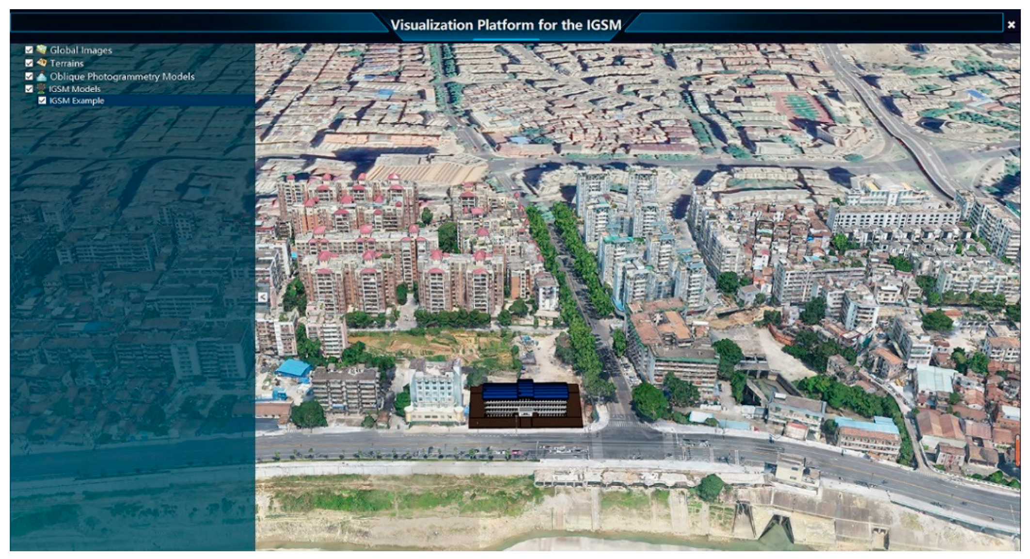
We selected the BIM sample data Office Building as the research subject to verify that the proposed IGSM can facilitate the spatial query and adjacent analysis function of the cellular spaces. We transformed the BIM model into IGSM through the modeling algorithm in Section 3.2 according to the model organization in Section 3.1. We then added the data to the 3D GIS platform, whose results are shown in Figure 14 and Figure 15.

Figure 14 shows the overall display effect of the IGSM in the 3D GIS platform. The tree list on the left column displays the loaded data types, including the terrain, image, and oblique model data. Figure 15 depicts the close-up display effect of the IGSM in the scenarios presented in the 3D GIS platform. Because the IGSM places a real location in the 3D GIS platform, we can obtain the geographic coordinates of any position on IGSM in the virtual environment. For example, the yellow box displays the spatial location obtained by the current mouse. The red box depicts the parameter $Params$ of the geographic location mapping algorithm. This also shows the validity of the model as a visual representation of buildings in an outdoor environment.

As an indoor GIS model, the IGSM has the functions of spatial query and analysis of cellular spaces (i.e., IGSMSpace). The following examples show the detailed description.

4.1.1. Spatial Query of Cellular Spaces in 3D Buildings

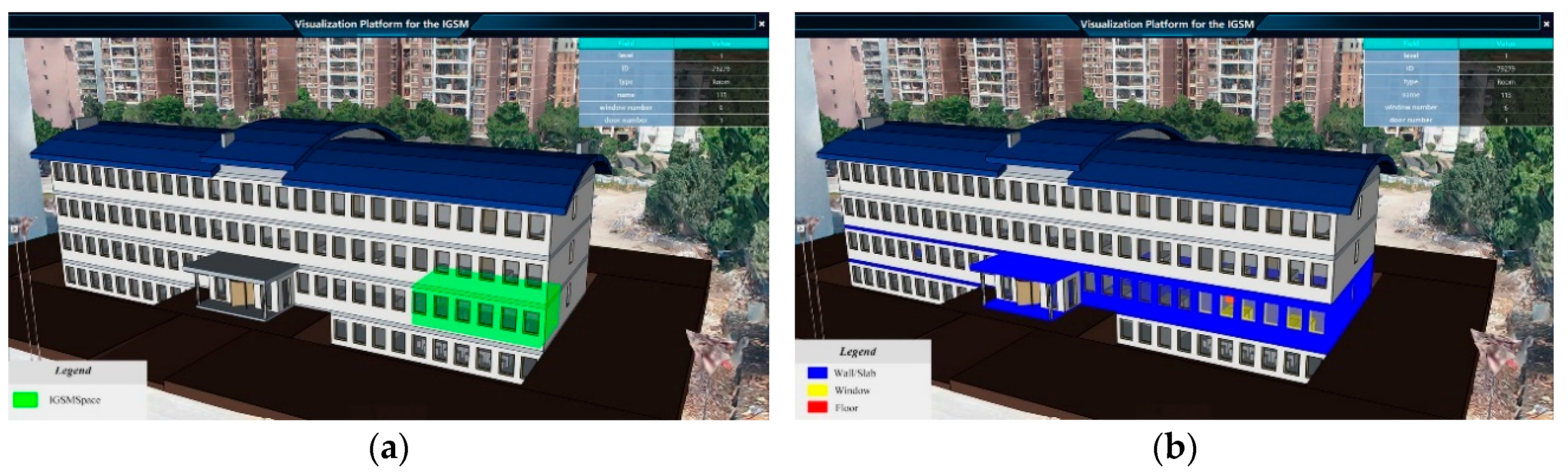
This example shows the spatial query and visualization validity of the IGSM in the 3D GIS platform. We can obtain the attributes corresponding to the cellular space in the IGSM by clicking on the spatial information corresponding to the IGSM in the platform.

As shown in Figure 16, by selecting the space of interest on the IGSM, the spatial information can be shown on the platform. Among them, the right floating window in the 3D GIS platform displays relevant attributes such as the level, name, and type of corresponding IGSMSpace (e.g., room and corridor). The selected space on the IGSM is highlighted in two ways below: Figure 16a highlights the IGSMSpace in a green translucent mode by removing the depth test; Figure 16b highlights building elements composed of the IGSMSpace. Besides, the IGSMSpace corresponds to a unique type and a name, the cellular space also can be located and visually expressed through the attribute query in the GIS platform (e.g., entering room 203).

4.1.2. Adjacent Query and Analysis of Cellular Spaces in 3D Buildings

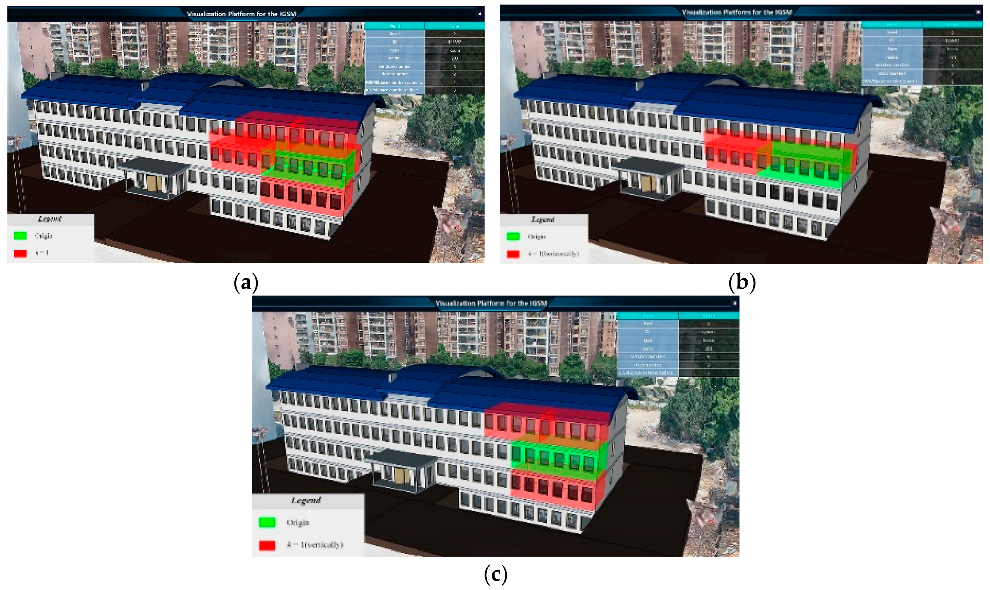
The example shows the adjacent query and analysis validity of the IGSM combined K-adjacent analysis algorithm. Figure 17a shows the result of the adjacent query. For instance, when query potential spaces near “Room 200”, we need to get adjacent spaces. Concretely, we can get “Room 200” by spatial query (Section 4.1.1). Then, according to the adjacency relations of the IGSM, we can get adjacent spaces, as shown in the below figure. Among them, Figure 17b shows the query result on the same floor, which is usually applied to the indoor location query. Figure 17c shows the query result of cellular spaces on the adjacent floor.

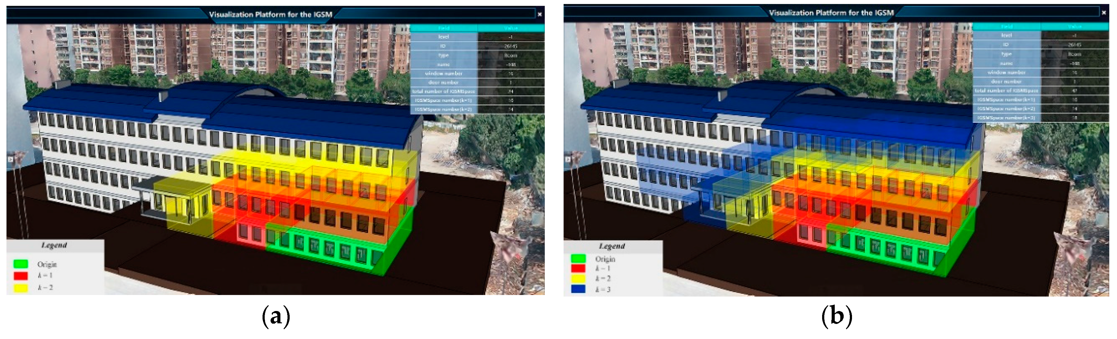
For the potential application of indoor noise pollution or emergency response, it is necessary to get the cellular spaces for decision support. Therefore, the indoor adjacency of the IGSM can be used to find the adjacent cellular spaces quickly. As shown in Figure 18, we can obtain the cellular spaces of different adjacent degrees through the K-adjacent analysis algorithm.

4.2. Performance

The abovementioned three types of experimental data were used to analyze and verify the modeling efficiency of the proposed indoor GIS modeling algorithm. According to Section 3.2, the IGSM modeling algorithms could be divided into three algorithms, which were experimentally examined herein.

4.2.1. Performance of the Geographical Location Mapping Algorithm

The geographic location mapping algorithm was achieved by the $Params$ when the IGSM was added to the 3D GIS platform. The parameter could be viewed and modified in real-time by adjusting the dialog box through the IGSM (red box, Figure 15). Therefore, the processing time of parameter calculation was counted when adding the IGSM to the 3D GIS platform during the experiment. The runtime of each model was counted multiple times to obtain an accurate processing time, and the mean value was obtained.

Table 3. Runtime of the geographical location mapping algorithm at different models.

Name	Number of Floors	Entity Number	Runtime (ms)
FZK Haus	2	14268	0.00482
Office Building	5	147712	0.00537
Office Building2	3	9169	0.00711

shows the runtime statistics through the processing time statistics of the three models.

The statistical analysis suggested that the geographic location mapping algorithm had a high processing efficiency. The algorithm runtime was unrelated to the model size because the geographic location mapping algorithm depended on the matrix calculation efficiency. Thus, the processing time of the algorithm was negligible.

4.2.2. Performance of the Floor Relation Extraction Algorithm

The floor relation extraction algorithm was used to establish the IGSMBuildingStorey, which mainly generates the floor number. In the experiment, the three BIM models were processed by the algorithms separately, and the processing time was counted. Besides, the runtime of each model was counted multiple times to ensure the accuracy of the processing time. The mean value was also taken.

Table 4. Runtime of the floor relation extraction algorithm at different models.

Name	Number of Floors	Runtime (s)
FZK Haus	2	0.0064
Office Building	5	1.5075
Office Building2	3	0.0120

presents the runtime statistics.

The statistical analysis suggested that the algorithm can quickly establish the floor number, with a runtime of less than 2 s. The algorithm runtime was related to the total number of the floor, which extended with the increase in the level number.

4.2.3. Performance of the Indoor Adjacency Extraction Algorithm

The indoor adjacency extraction algorithm was used to establish the IGSMSpace by obtaining indoor adjacency relations of each cellular space. Besides, the adjacency relations between the IGSMSpace were measured by setting a specific image resolution because different image resolutions can affect the processing efficiency of the algorithm; hence, the processing time of the algorithm for different image resolutions was considered in this experiment. Vertical surface information (e.g., wall) can be displayed in the image to ensure the validity of the algorithm. Therefore, the maximum image resolution was set to 0.5 m, assuming the wall thickness was greater than 0.5 m.

Figure 19 shows the statistical result of the indoor adjacency extraction algorithm, according to 10 types of different image resolutions set at 0.5 m intervals: the three types of experimental data were processed, and the processing time and total number of pixels of the algorithm were then calculated.

The statistical analysis suggested that the indoor adjacency extraction algorithm can quickly establish the spatial information of IGSMSpace elements, with a runtime less of than 2 s. The runtime of the algorithm remained unchanged when the image resolution was greater than 0.1 m; however, the runtime was significantly prolonged when the resolution was 0.05 m (Figure 19b). This is attributed to the three times increase in the total number of pixels when the image resolution decreased from 0.1 to 0.05 m, which increased the processing time of the algorithm. The total number of pixels did not change significantly when the image resolution was greater than 0.1 m, therefore the algorithm runtime remained the same.

Combined with the runtime and the actual wall width, we used images with 0.1 m resolution to quickly establish the spatial information of the IGSMSpace elements. The runtime of the three models was maintained within 0.4 s.

In summary, we adopted three typical BIM models in the experiment and statistically analyzed the runtime of the modeling algorithms. The experimental results revealed that the proposed method can rapidly transform a BIM model into an IGSM.

5. Discussions

In the study, we developed a method for the automated generation of indoor GIS models based on BIM models to support adjacent analysis of indoor spaces. The method included three steps. Firstly, we devised a new indoor GIS model (i.e., IGSM) to form the complete indoor spatial feature; mainly, the indoor adjacency of IndoorGML was integrated into the BIM model. Then, according to the designed model, we proposed a modeling algorithm that realizes the automated rapid generation of the IGSM from the BIM model. Finally, for the potential application in the 3D GIS, we proposed the K-adjacent analysis algorithm to improve the ability of adjacent analysis of indoor spaces.

The experiment results suggested the validity and modeling performance of the method: (1) For the validity of the IGSM, the effectiveness of the model in the GIS environment (including visualization, spatial query, and adjacent analysis) was illustrated by combining the generated IGSM with the K-adjacent analysis algorithm in the experiment. (2) For the modeling performance we selected three general BIM Models as the experimental objects, testing the performance of the modeling algorithms respectively, and suggested that the algorithms are rapid and reusable, which can be applied to other general BIM models. The experiment results can demonstrate the replicability of the method as well.

Compared with the current methods, the advantages of the method are mainly displayed in the following aspects.

For the indoor GIS model, the IGSM proposed in the paper had the geometric and semantic information of the BIM model, which also incorporated the basic spatial feature of indoor GIS. Different from other indoor GIS models, the model had the necessary indoor adjacency relations of cellular spaces, which supplemented the spatial characteristics of the indoor GIS model and laid the foundation for subsequent indoor query and analysis functions.

For the modeling algorithms, according to the characteristics of the BIM model, we put forward a modeling algorithm for building an indoor GIS model from the BIM model. The modeling algorithms mainly describe a georeferenced algorithm in detail, and make up for the fact that the existing methods do not have an adjacency relations extraction method suitable for the BIM model. The modeling algorithms have the features of automation and rapid.

For the indoor spatial analysis and application: based on the IGSM model, we proposed a K-adjacent analysis algorithm, which extended the model from the basic adjacent query or analysis to the analysis of the cellular space with different adjacent degrees. The algorithm can be applied to the assistant decision-making of the indoor emergency response (such as obtaining the relevant spaces of different influenced degrees of a fire space), which extended the application ability of the adjacent analysis of indoor GIS.

At present, the method proposed in this paper retains the feature of the BIM model itself (connectivity relations), so it has the potential of navigation analysis. The method is mainly aimed at the general building model, considering that the indoor space structure will continue to evolve, which forms a certain challenge for the modeling algorithms. Therefore, improving the robustness of the method and realizing the subsequent indoor and outdoor path navigation and other applications are our next research focus. The following need to be focused on in the future: (1) For visualization, when enormous BIM models integrate into the GIS environment, the visualization burden limits subsequent applications. Therefore, some visualization strategies (such as LODs of CityGML and culling algorithms) need to be considered to build an efficient BIM-GIS visualization system. (2) For the integration from BIM to GIS, the geographical location mapping algorithm considered that the Z-axis of the local coordinate system of the BIM model was perpendicular to the normal vector of the ellipsoid, but there may exist errors in practice. Meanwhile, the transformation error and the indoor location strategy need to be discussed more clearly as well. Therefore, it is necessary to explore a more accurate positioning method combing location equipment to ensure the accurate application of the model in the GIS environment.

References

- Ma, Z.; Ren, Y. Integrated Application of BIM and GIS: An Overview. Procedia Eng. 2017, 196, 1072–1079. [Google Scholar] [CrossRef]
- Song, Y.; Wang, X.; Tan, Y.; Wu, P.; Sutrisna, M.; Cheng, J.; Hampson, K. Trends and Opportunities of BIM-GIS Integration in the Architecture, Engineering and Construction Industry: A Review from a Spatio-Temporal Statistical Perspective. ISPRS Int. J. Geo-Inf. 2017, 6, 397. [Google Scholar] [CrossRef] [Green Version]
- Wang, H.; Pan, Y.; Luo, X. Integration of BIM and GIS in sustainable built environment: A review and bibliometric analysis. Autom. Constr. 2019, 103, 41–52. [Google Scholar] [CrossRef]
- Cheng, J.; Deng, Y.; Du, Q. Mapping between BIM models and 3D GIS city models of different levels of detail. In Proceedings of the 13th International Conference on Construction Applications of Virtual Reality, London, UK, 30–31 October 2013; pp. 30–31. [Google Scholar]
- Rafiee, A.; Dias, E.; Fruijtier, S.; Scholten, H. From BIM to Geo-analysis: View Coverage and Shadow Analysis by BIM/GIS Integration. Procedia Environ. Sci. 2014, 22, 397–402. [Google Scholar] [CrossRef] [Green Version]
- Deng, Y.; Cheng, J.C.P.; Anumba, C. Mapping between BIM and 3D GIS in different levels of detail using schema mediation and instance comparison. Autom. Constr. 2016, 67, 1–21. [Google Scholar] [CrossRef]
- Amirebrahimi, S.; Rajabifard, A.; Mendis, P.; Ngo, T. A framework for a microscale flood damage assessment and visualization for a building using BIM–GIS integration. Int. J. Digit. Earth 2016, 9, 363–386. [Google Scholar] [CrossRef]
- Isikdag, U.; Zlatanova, S.; Underwood, J. A BIM-Oriented Model for supporting indoor navigation requirements. Comput. Environ. Urban Syst. 2013, 41, 112–123. [Google Scholar] [CrossRef]
- Zhou, X.; Zhao, J.; Wang, J.; Su, D.; Zhang, H.; Guo, M.; Guo, M.; Li, Z. OutDet: An algorithm for extracting the outer surfaces of building information models for integration with geographic information systems. Int. J. Geogr. Inf. Sci. 2019, 33, 1444–1470. [Google Scholar] [CrossRef]
- Lee, J. A Spatial Access-Oriented Implementation of a 3-D GIS Topological Data Model for Urban Entities. GeoInformatica 2004, 8, 237–264. [Google Scholar] [CrossRef]
- Taneja, S.; Akinci, B.; Garrett, J.H.; Soibelman, L. Algorithms for automated generation of navigation models from building information models to support indoor map-matching. Autom. Constr. 2016, 61, 24–41. [Google Scholar] [CrossRef] [Green Version]
- Lin, W.Y.; Lin, P.H. Intelligent generation of indoor topology (i-GIT) for human indoor pathfinding based on IFC models and 3D GIS technology. Autom. Constr. 2018, 94, 340–359. [Google Scholar] [CrossRef]
- ArcGIS Data Interoperability Extension. Available online: https://desktop.arcgis.com/en/arcmap/latest/extensions/data-interoperability/a-quick-tour-of-the-data-interoperability-extension.htm#ESRI_SECTION1_B21612BC4CF9425482836684FEDC0172 (accessed on 18 March 2020).
- Software Implementations. Available online: https://technical.buildingsmart.org/community/software-implementations/ (accessed on 18 March 2020).
- Afyouni, I.; Ray, C.; Claramunt, C. Spatial models for context-aware indoor navigation systems: A survey. J. Spat. Inf. Sci. 2012. [Google Scholar] [CrossRef] [Green Version]
- Kang, H.-K.; Li, K.-J. A Standard Indoor Spatial Data Model—OGC IndoorGML and Implementation Approaches. ISPRS Int. J. Geo-Inf. 2017, 6, 116. [Google Scholar] [CrossRef]
- Li, K.-J.; Conti, G.; Konstantinidis, E.; Zlatanova, S.; Bamidis, P. 10-OGC IndoorGML: A Standard Approach for Indoor Maps. In Geographical and Fingerprinting Data to Create Systems for Indoor Positioning and Indoor/Outdoor Navigation; Conesa, J., Pérez-Navarro, A., Torres-Sospedra, J., Montoliu, R., Eds.; Intelligent Data-Centric Systems; Academic Press: Cambridge, MA, USA, 2019; pp. 187–207. ISBN 978-0-12-813189-3. Available online: https://www.sciencedirect.com/science/article/pii/B9780128131893000101 (accessed on 21 August 2020).
- Lee, J.; Kwan, M.-P. A combinatorial data model for representing topological relations among 3D geographical features in micro-spatial environments. Int. J. Geogr. Inf. Sci. 2005, 19, 1039–1056. [Google Scholar] [CrossRef]
- Tashakkori, H.; Rajabifard, A.; Kalantari, M. A new 3D indoor/outdoor spatial model for indoor emergency response facilitation. Build. Environ. 2015, 89, 170–182. [Google Scholar] [CrossRef]
- Kolbe, T.H. Representing and Exchanging 3D City Models with CityGML. In 3D Geo-Information Sciences; Lee, J., Zlatanova, S., Eds.; Springer Berlin Heidelberg: Berlin, Heidelberg, 2009; pp. 15–31. ISBN 978-3-540-87395-2. [Google Scholar]
- Gröger, G.; Plümer, L. CityGML—Interoperable semantic 3D city models. ISPRS J. Photogramm. Remote Sens. 2012, 71, 12–33. [Google Scholar] [CrossRef]
- De Laat, R.; van Berlo, L. Integration of BIM and GIS: The Development of the CityGML GeoBIM Extension. In Advances in 3D Geo-Information Sciences; Kolbe, T.H., König, G., Nagel, C., Eds.; Springer: Berlin/Heidelberg, Germany, 2011; pp. 211–225. ISBN 978-3-642-12669-7. [Google Scholar]
- Van den Brink, L.; Stoter, J.; Zlatanova, S. Establishing a national standard for 3D topographic data compliant to CityGML. Int. J. Geogr. Inf. Sci. 2013, 27, 92–113. [Google Scholar] [CrossRef]
- Donkers, S.; Ledoux, H.; Zhao, J.; Stoter, J. Automatic conversion of IFC datasets to geometrically and semantically correct CityGML LOD3 buildings: Automatic conversion of IFC datasets to CityGML LOD3 buildings. Trans. GIS 2016, 20, 547–569. [Google Scholar] [CrossRef] [Green Version]
- Biljecki, F.; Ledoux, H.; Stoter, J. An improved LOD specification for 3D building models. Comput. Environ. Urban Syst. 2016, 59, 25–37. [Google Scholar] [CrossRef] [Green Version]
- Liebich, T. IFC4—The New BuildingSMART Standard. In Proceedings of the IC Meeting; bSI Publications: Helsinki, Finland, 2013. [Google Scholar]
- ESRI ArcGIS & FME. Available online: https://www.safe.com/solutions/technology/esri-arcgis/ (accessed on 18 March 2020).
- Xu, M.; Hijazi, I.; Mebarki, A.; Meouche, R.E.; Abune’meh, M. Indoor guided evacuation: TIN for graph generation and crowd evacuation. Geomat. Nat. Hazards Risk 2016, 7, 47–56. [Google Scholar] [CrossRef] [Green Version]
- Teo, T.-A.; Cho, K.-H. BIM-oriented indoor network model for indoor and outdoor combined route planning. Adv. Eng. Inform. 2016, 30, 268–282. [Google Scholar] [CrossRef]
- Chen, L.-C.; Wu, C.-H.; Shen, T.-S.; Chou, C.-C. The application of geometric network models and building information models in geospatial environments for fire-fighting simulations. Comput. Environ. Urban Syst. 2014, 45, 1–12. [Google Scholar] [CrossRef]
- Uggla, G.; Horemuz, M. Geographic capabilities and limitations of Industry Foundation Classes. Autom. Constr. 2018, 96, 554–566. [Google Scholar] [CrossRef]
- Arroyo Ohori, K.; Diakité, A.; Krijnen, T.; Ledoux, H.; Stoter, J. Processing BIM and GIS Models in Practice: Experiences and Recommendations from a GeoBIM Project in The Netherlands. IJGI 2018, 7, 311. [Google Scholar] [CrossRef] [Green Version]
- Diakite, A.A.; Zlatanova, S. Automatic geo-referencing of BIM in GIS environments using building footprints. Comput. Environ. Urban Syst. 2020, 80, 101453. [Google Scholar] [CrossRef]
- Zhang, T.; Suen, C.Y. A fast parallel algorithm for thinning digital patterns. Commun. ACM 1984, 27, 236–239. [Google Scholar] [CrossRef]
- IFC++. Available online: http://www.ifcquery.com/ (accessed on 18 March 2020).
- osgEarth. Available online: http://osgearth.org/ (accessed on 18 March 2020).
Figure 1.
One ‘green’ wall can be shared by multiple IfcSpace objects. (a) The BIM model named FZK Haus. (b) The BIM model named Office Building.
Figure 2.
The levels of detail (LODs) of CityGML (image from Biljecki et al. [25]).
Figure 3.
Workflow of the proposed method.