Methods for Inferring Route Choice of Commuting Trip From Mobile Phone Network Data


1
Department of Computer Engineering, Faculty of Engineering, Chiang Mai University, Chiang Mai 50200, Thailand
2
Excellence Center in Infrastructure Technology and Transportation Engineering, Department of Computer Engineering, Faculty of Engineering, Chiang Mai University, Chiang Mai 50200, Thailand
3
Sociology and Economics of Networks and Services Department, Orange Labs, 92320 Châtillon, France
4
SENSEable City Laboratory, Massachusetts Institute of Technology, Cambridge, MA 02139, USA
*
Author to whom correspondence should be addressed.
ISPRS Int. J. Geo-Inf. 2020, 9(5), 306; https://doi.org/10.3390/ijgi9050306
Submission received: 30 March 2020
/
Revised: 30 April 2020
/
Accepted: 4 May 2020
/
Published: 7 May 2020
Abstract
:For billing purposes, telecom operators collect communication logs of our mobile phone usage activities. These communication logs or so called CDR has emerged as a valuable data source for human behavioral studies. This work builds on the transportation modeling literature by introducing a new approach of crowdsource-based route choice behavior data collection. We make use of CDR data to infer individual route choice for commuting trips. Based on one calendar year of CDR data collected from mobile users in Portugal, we proposed and examined methods for inferring the route choice. Our main methods are based on interpolation of route waypoints, shortest distance between a route choice and mobile usage locations, and Voronoi cells that assign a route choice into coverage zones. In addition, we further examined these methods coupled with a noise filtering using Density-Based Spatial Clustering of Applications with Noise (DBSCAN) and commuting radius. We believe that our proposed methods and their results are useful for transportation modeling as it provides a new, feasible, and inexpensive way for gathering route choice data, compared to costly and time-consuming traditional travel surveys. It also adds to the literature where a route choice inference based on CDR data at this detailed level—i.e., street level—has rarely been explored.
1. Introduction
The majority of trips made by individuals is commuting, which is the most regular and repeated travel between a residence and workplace. Commuting is thus believed to be one of major causes of traffic congestion [1]. Understanding commuting patterns is thus essential and can play an important role in urban planning and traffic management. Due to its nature, commuting patterns and behaviors have been investigated in the fields of human geography, transport, and urban studies. Today, however, commuting as well as mobility patterns are becoming a more attractive research problem to scholars from other disciplines—such as physics, statistics, and data science—because of recent availability of large-scale electronic datasets from which different models can be examined and developed to better describe characteristics of human mobility at various spatial scales.
From the transportation’s perspective, human mobility as seen in forms of collective trips is studied in the domain of travel demand modeling for which the sequential four-step model [2] traditionally has been utilized for transportation forecasts, such as estimating the number of vehicles on a planned road, the ridership on a railway line, and the number of bus passengers at the airport. The four-step model consists of trip generation, trip distribution, mode choice, and route assignment, where each of these steps is designed to model the amounts, locations, travel modes, and route choices of generated trips, respectively.
Travel demand modeling begins with the collection of traffic data that is related to travel behavior—e.g., traffic count, number of trips made from/to a particular place, and start/end times of journeys. Traditionally, traffic data is collected by a survey of individual travel behavior. Information about the individual, their household, and a diary of their journeys on a given day are typically collected by most surveys. Normally, methods for a travel survey are traffic count, roadside interviews, and questionnaires, which are costly and laborious [3] and thereby major travel surveys are usually conducted once a decade. Due to this large gap between the surveys, the collected data can be outdated despite the fact that it provides detailed mobility information. Its high cost also limits travel survey being done within particular analysis zones that cause spotty data. Moreover, the collected data is often based on survey participants’ recalling some information regarding their past journeys, which can also be erroneous due to the inaccurate responses to the travel survey questionnaires.
Due to recent advances in location-aware technologies, sensors such as GPS tracking units have been used increasingly for travel surveys [4]. However, collecting data at such a large scale is difficult and challenging because of the privacy issues and regulations, e.g., the EU general data protection regulation (GDPR) [5]. Recent attempts have produced data that are limited to specific type of tracked individuals, such as college students [6], city cyclists [7], and customers of a provided service [8]. Nonetheless, privacy concerns still largely prevent this type of detailed mobility data to be available and utilized extensively for travel demand modeling.
Recently, opportunistic sensing data produced from various sources has emerged as a promising alternative that can provide insights about spatial distribution of human mobility. Opportunistic data refers to data that originally is collected for one purpose but also creates an opportunity for another purpose. Mobile phone network data or so called CDR (call detail records) is a kind of the opportunistic sensing data where the data is purposely collected for customer billing, but it can also be useful for human mobility studies. CDR is a log of cellular network connectivity of a mobile phone user. Each time the mobile phone user connects to a serviced cellular network by receiving or making a call or using internet, the communication information is recorded—i.e., call duration, timestamp, caller’s and callee’s identifications, and location of connected cellular tower. Collectively, with these individual location footprints, CDR has emerged as a useful data source in human mobility studies [9,10]. Though the CDR data is not as detailed as GPS tracking data, it is worth noting that there is still a privacy concern even if they are anonymized when analyzed rigorously with additional outside information [11].
In the context of the four-step model, the CDR data has been used in each of the sequential steps. In the trip generation step, it has been used for—among other things—inference of trip volume and spatial distribution for estimating commuting tip generation rates [12], calibration of a hybrid trip generation model [13], and estimation of zonal travel demand [14]. It has been used in several studies in the trip distribution step, such as origin–destination (O-D) matrix’s construction [15,16,17], evaluation [18], and modeling [19,20,21]. In the mode choice step, the CDR data has been used for inferring commuting mode choice based on distance measures between visited cell towers and route choices [22], transport mode of given origin and destination based on travel time [23], and commuting transport mode based on weak-labeling of visited cell towers [24]. Due to its challenging nature of the problem, there are very few studies reported on using CDR data in the route assignment step, which is the most detailed level of the transportation in all four steps. These studies include a simulation-based approach for route choice estimation by Tettamanti et al. [25], but with drawbacks in its feasibility in real-world scenarios where CDR data is spatially much more coarse-grained and sparse than in its simulated situation. Another work is by Breyer et al. [26], which is an approach to reconstruct used routes based on CDRs; however, its shortcomings are the case that only one route can be estimated per visited cellular zone. Lastly, a work by Bwambele et la. [27] is an attempt to model route choice behavior, but for long-distance trips at an inter-regional level. While other previous studies have captured commuting patterns at a zonal scale such as clustered areas [28], cellular tower locations [29], and grid cells [30], this study attempts to extend the literature and fill in the gap by proposing and evaluating models for inferring commuting route choice at street level based solely on a CDR data.
2. Materials and Methods
2.1. Data Description
CDR is a set of individual mobile phone communication logs, collected by a telecom operator for billing purposes. Each time that a mobile phone user connects to his/her subscribed cellular network by making or receiving a call, a communication log is recorded. Each record contains caller ID, callee ID, caller’s connected cell tower ID, callee’s connected cell tower ID, timestamp, and call duration. A connected cell tower is the serving cell tower, which is the nearest tower or base station to the user.
In this study, we used CDR data collected from 1.8 million mobile phone users over a course of one calendar year in Portugal, from April 2006 to March 2007. To safeguard personal information, individual phone numbers were anonymized by the operator before leaving their storage facilities, and were identified with a security ID (hash code), which complies with the EU GDPR. We treated data on a securitized machine, under the Article 89 GDPR exemption for research which allows personal data treatment for research purposes. For our study, as we were interested in analyzing the users’ mobility, we selected a set of mobile users whose cellular network connections were at least five times a month and communication activities were observed for each of the 12 months to ensure a fine-grained mobility observation. This filtering yielded us 110,213 users, who were our study’s subjects [31]. There is a total of 6511 cell towers in our dataset. Each cell tower has a unique ID with its corresponding geo-location (latitude and longitude).
2.2. Home and Work Location Inference
We were particularly interested in the commuting trip, whose origin and destination are home and workplace (or school). Thus, the first information that we needed before we can further investigate the route choice was the home and workplace locations of each subject. We adopted the approach utilized in previous studies [22,31,32] to infer each individual subject’s home location as the cell tower’s location that was used most frequently (highest connectivity) during the sleeping hours (10:00 p.m.–7:00 a.m.) over the 12-month period. Likewise, the workplace location is inferred as the location of the cell tower that was most frequently used during the office hours (9:00 a.m.–5:00 p.m.) on weekdays.
2.3. Route Choices
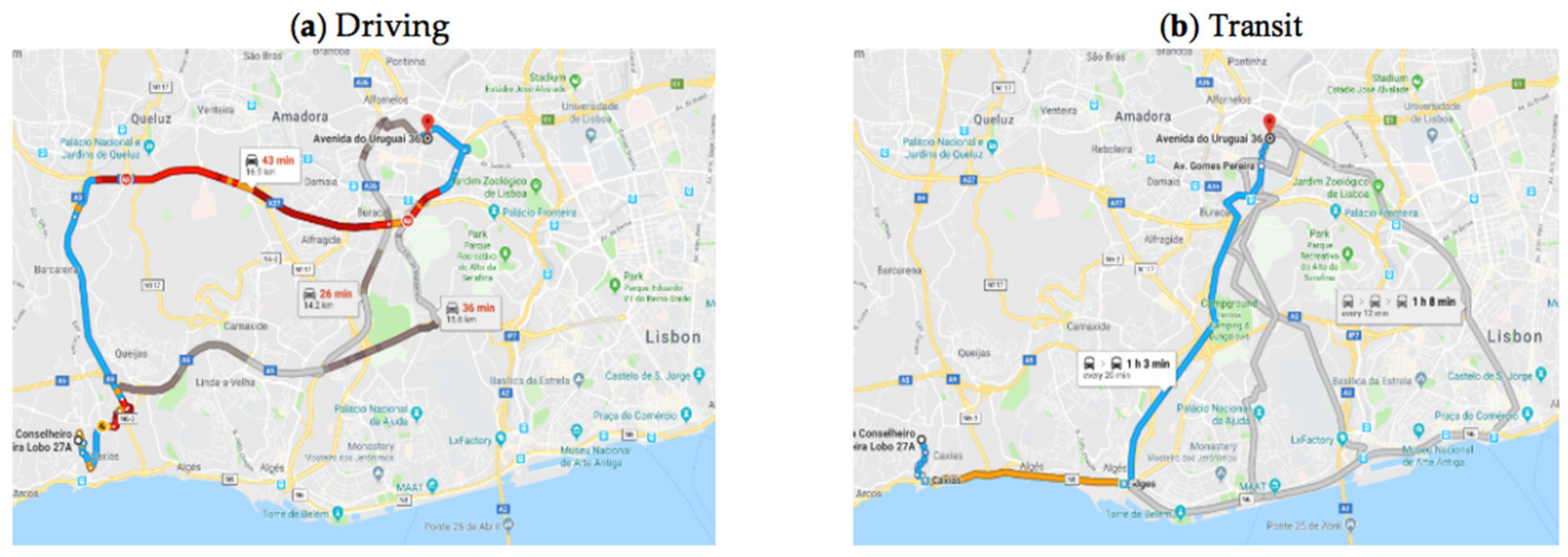
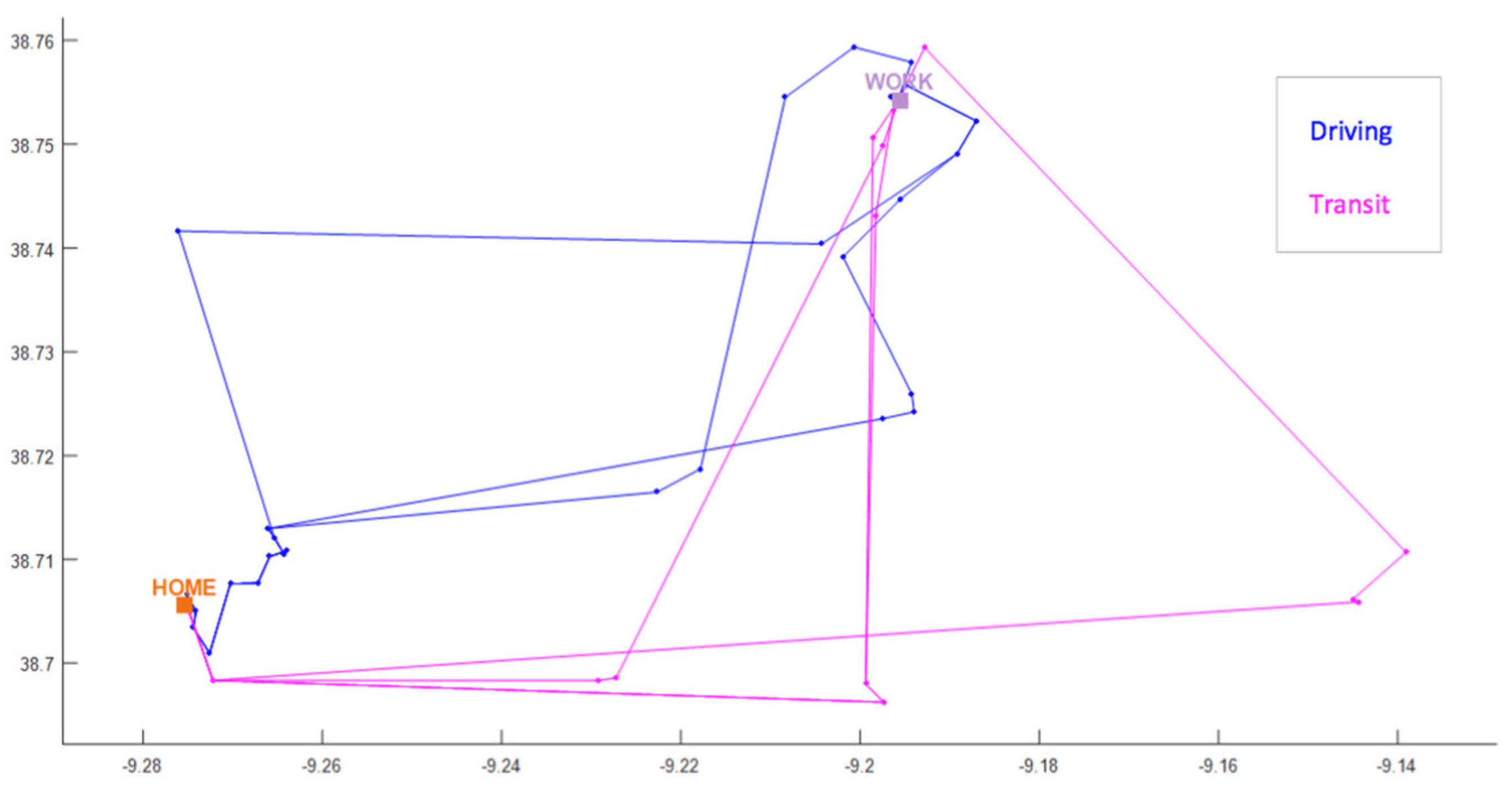
Once the home and workplace locations of each subject are inferred, a set of potential route choices are obtained from the use of the Google Maps Directions API. As there are many route choices between home and workplace, the Google Maps Directions API provides us with a set of potential realistic route choices with our given set of origin and destination, which are the inferred home and workplace locations [33,34,35,36]. Through the API, we requested possible route choices by car and public transit for each subject. An example of possible route choices displayed in Google Maps is shown in Figure 1. With our HTTP request for the route choices through the Google Maps Directions API, we received a set of waypoints—i.e., a sequence of geo-coordinates along the route choice. Each route choice can have a different number of waypoints depending on the shape of the route. Curvier routes have more waypoints. The waypoints received from the route choices shown in Figure 1 are illustrated in Figure 2.
2.4. Route Choice Inference
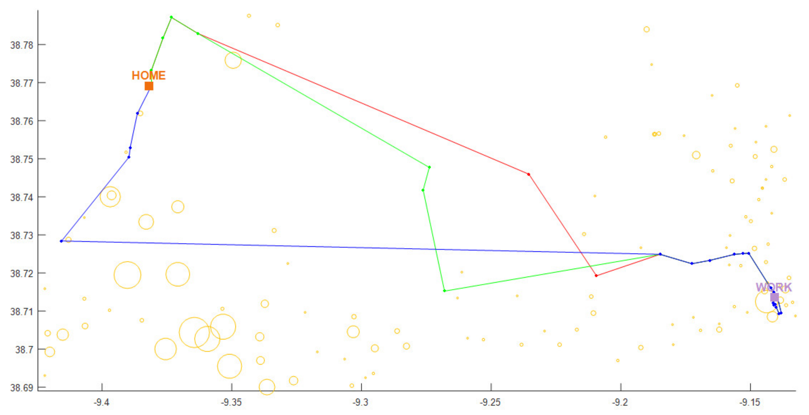
With the obtained set of possible route choices, our task was to identify the route that was most likely taken by the subject from his/her mobile phone usage pattern. An example of a subject is shown in Figure 3, where there are three possible route choices between home and workplace. Each yellow circle represents a location of the used/connected cell tower over the observed 12-month period, while its size corresponds to the total amount of connections—i.e., the larger the circle, the more frequently visited the location. Our task can then be systematically formulated as a problem of choosing the route that is nearest to the circles (visited locations).
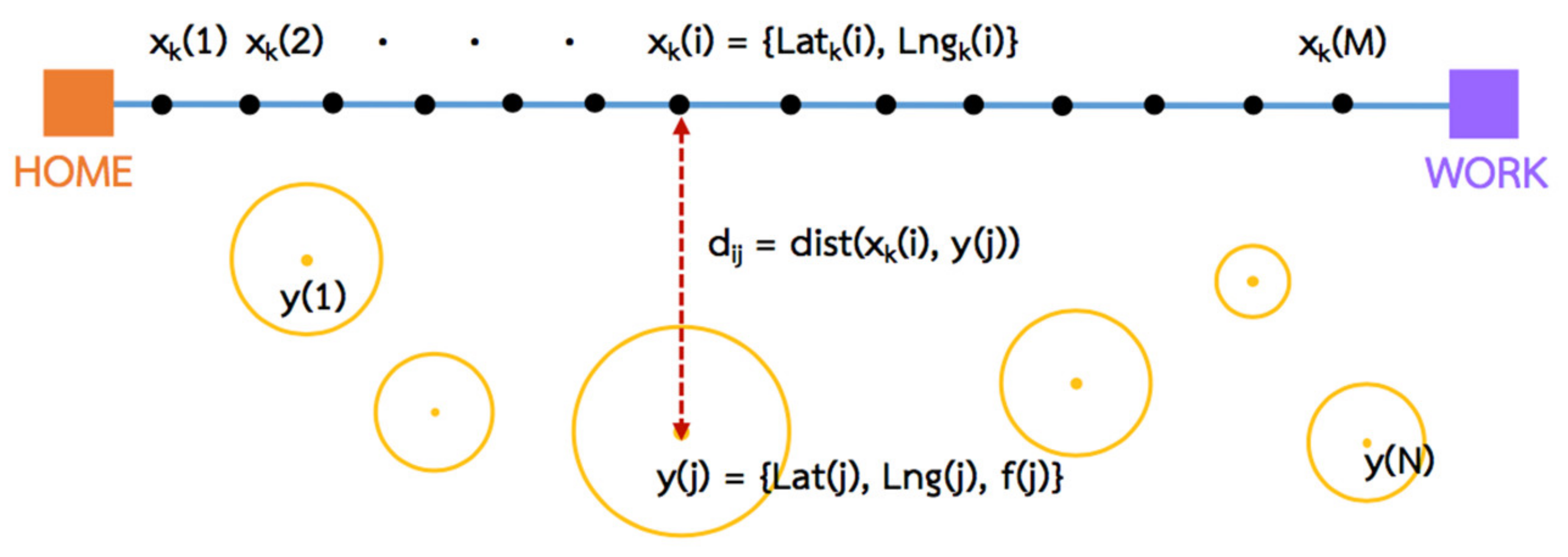
Intuitively, our approach is to find the likelihood of a route choice being chosen based on some calculated value measured between it and all visited cell towers with also taking into account the amount of visits. Therefore, let denote a set of waypoints of route choice k, i.e., where each waypoint i, i.e., contains a pair of geo-location coordinates; latitude and longitude. The likelihood score of route k (Wk) can be calculated as a sum of ratios of the number of visits to the geographical distance from route k to each visited tower location,
where M is the total number of waypoints and , where N is the total number of visited cell towers, f(j) is the total number of visits to cell tower j, and is the geographical distance (in km) between a waypoint i and cell tower j based on the Haversine formula, as follows.
where the geo-coordinates of cell tower j is and R is the Earth radius (6371 km). Figure 4 shows a graphic that illustrates our distance calculation approach where black dots between the home and workplace represent waypoints and circles are the visited cell tower locations. Essentially, the route choice with the maximum likelihood score (Wk) is identified as the chosen one among all candidates, i.e., .
2.4.1. Interpolation-Based Method
The number of waypoints of each route choice can be different depending upon the shape of the route. Curvier routes contain more waypoints. Hence, a route with more waypoints can potentially have a higher likelihood score (Wk) as it sums over a higher number of terms (M) i.e., waypoints. To have a fairer comparison across all route choice candidates, an interpolation is applied to equalize the number of waypoints of each route. With an equal number of waypoints, each route can be divided into the same number of segments (or edges), as shown in Figure 5.
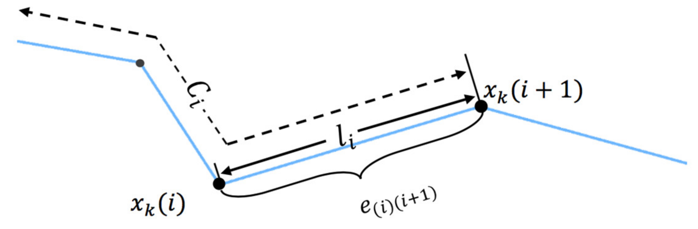
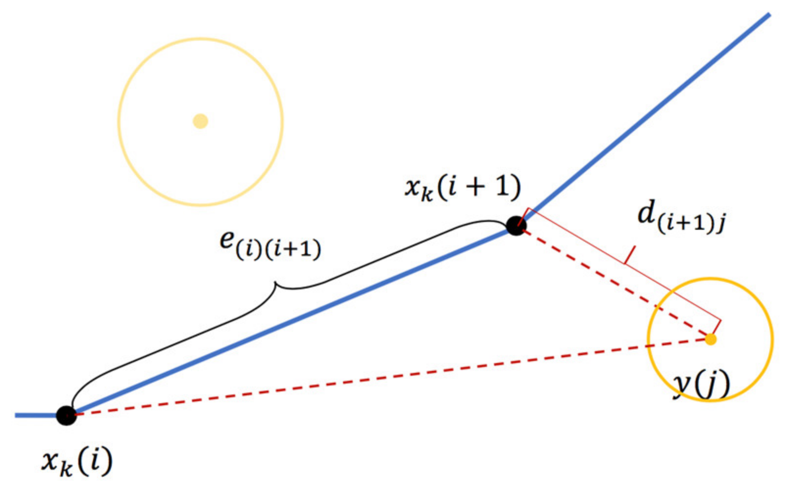
To obtain a set of interpolated waypoints, we firstly need to find a set of edges or road segments that constitutes the whole route. Each edge that connects two adjacent interpolated waypoints contains information about the locations of adjacent waypoints, its slope, length, and accumulated distance from the origin (i.e., home). Let xk(i) and xk(i+1) denote adjacent waypoints of edge e(i)(i+1) that has a slope of mi with length li, and has a cumulative distance from the origin of Ci. Figure 6 shows a graphic illustrating physical meaning of these variables. Systematically, a given input is a set of route’s original waypoints , and the desired output is a set of edges of the route . This process of obtaining a set of route edges is described in the Algorithm 1.
| Algorithm 1: To obtain a set of route edges. |
| Input: Route waypoints, |
| Output: Set of route edges, |
| 1 for to do |
| 2 |
| 3 |
| 4 |
| 5 |
| 6 end for |
| 7 |
| 8 return |
Once a set of edges is obtained by using the Algorithm 1, we can then use this edge information to interpolate the route by adjusting the edge length and locations according to a required new number of edges. The process starts with a new interpolated edge length (), which can be simply calculated as a ratio of the whole route length and a required new number of edges (t)—i.e., the new number of road segments along the route. A new waypoint is assigned based on the original waypoint locations and the new interpolated edge length. Figure 7 shows an example where an original route with five waypoints (four edges) is interpolated into four waypoints (three edges). Our method is described formally by the Algorithm 2.
| Algorithm 2: To obtain interpolated route waypoints. |
| Input: Route edges ( and number of interpolated edges (Output: Interpolated route waypoints, |
| 1 for to do |
| 2 |
| 3 |
| 4 if |
| 5 |
| 6 |
| 7 else |
| 8 |
| 9 |
| 10 end if |
| 11 |
| 12 end for |
| 13 Return |
2.4.2. Shortest Distance-Based Method
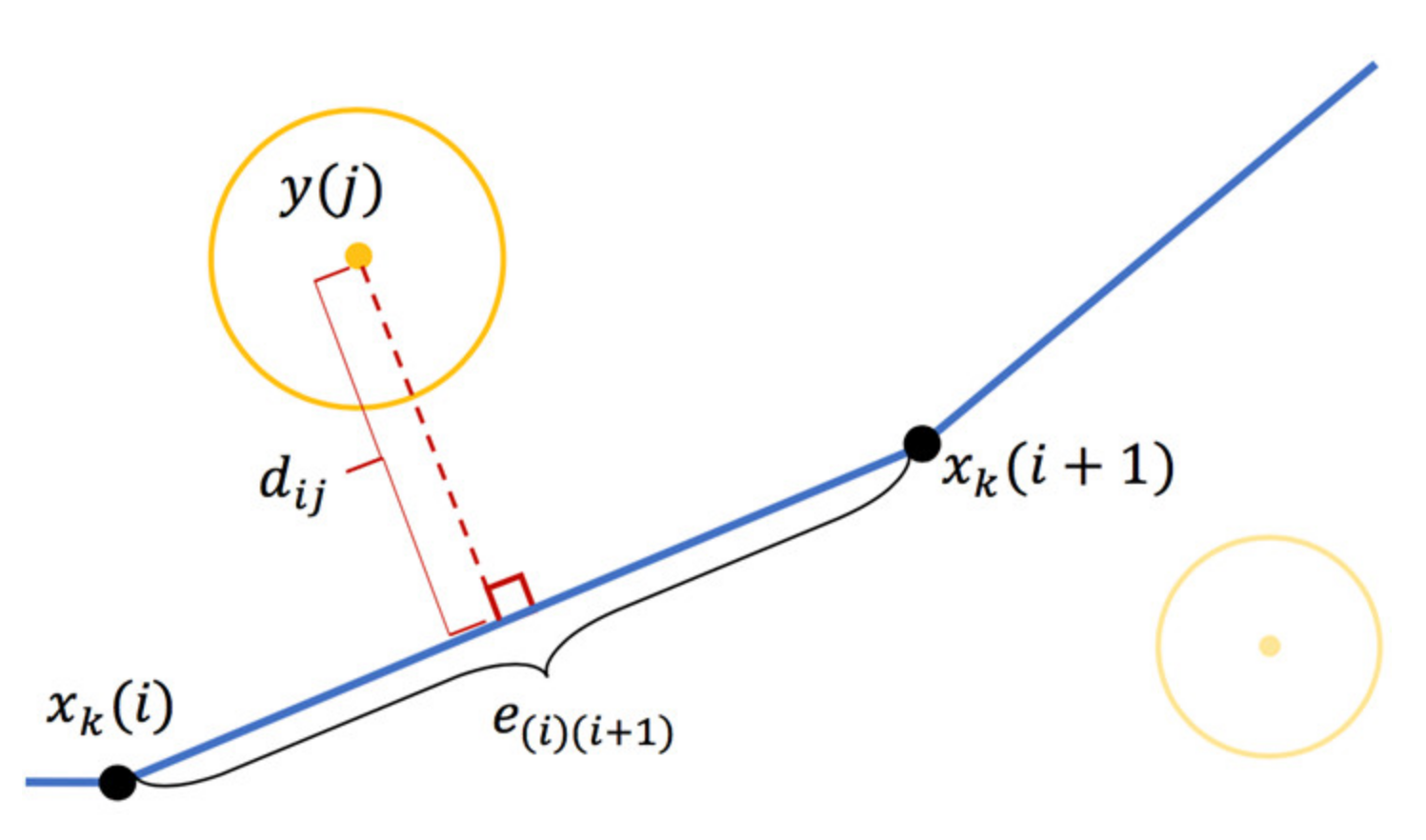
Another approach to measuring distance from the route to the visited cell tower locations is to find the shortest distance between each visited cell tower location and each route segment or edge (e(i)(i+1)) instead of the distance to each waypoint (xk(i)). Intuitively, this approach helps better reflect on a more realistic distance from the route to the visited cell tower.
With this approach, the distance dij in Equation (2) can therefore be calculated as a distance from a visited cell tower location y(j) that is perpendicular to an edge e(i)(i+1) —i.e., shortest distance. If there is no perpendicular distance from y(j) to e(i)(i+1), then dij is a distance from y(j) to either adjacent waypoint (xk(i) or xk(i+1)) whichever is the shortest. Figure 7 shows illustrating graphic example of a case where there is a perpendicular distance from a visited cell tower location to the edge. On the other hand, Figure 8 shows an example of another scenario where there is no perpendicular distance along the edge, so the distance dij is calculated as a distance between the visited cell tower and the nearest waypoint of the considered edge.
Practically, as we operate in a discrete domain, locating a point along the edge that projects a perpendicular distance to a visited cell tower can be done approximately by interpolating the edge and finding the point with the shortest distance to the cell tower. The number of interpolated points along an edge can be set such that it gives a reasonable separation between the points for which we used one-meter spacing. Hence, number of interpolated points along an edge can be calculated as for each edge. With a given edge and its calculated number of interpolated points (t’), the Algorithm 2 can be applied to obtain the interpolated points along the edge from which the shortest distance can be then be estimated. Algorithm 3 describes our method of obtaining a shortest distance, where is a set of interpolated points along the edge i.
| Algorithm 3: To find a shortest distance. |
| Input: Edge and cell tower |
| Output: Shortest distance, |
| 1 |
| 2 |
| 3 for to do |
| 4 |
| 5 end for |
| 6 Return |
2.4.3. Voronoi Cell-Based Method
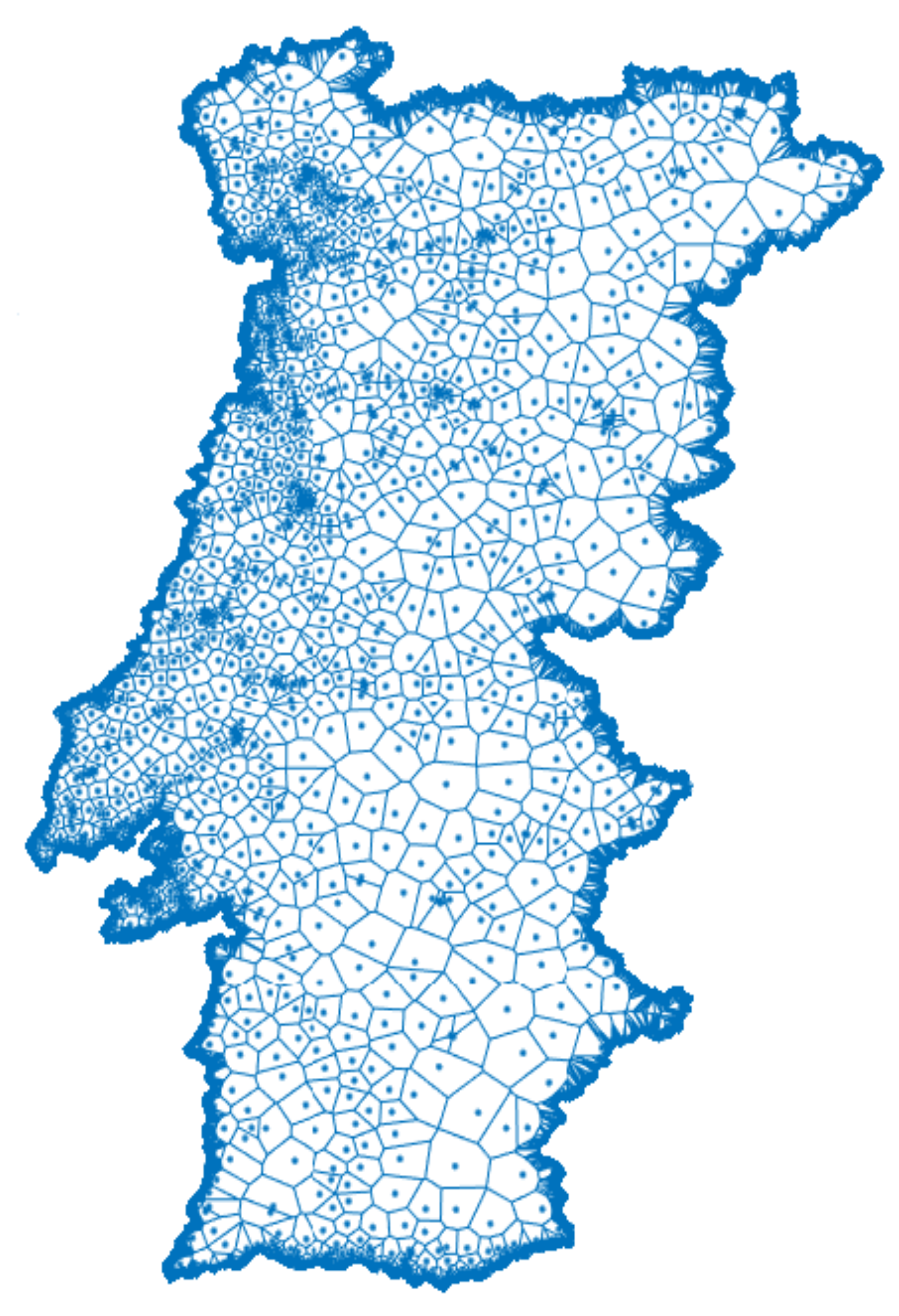
Voronoi diagram is a popular method for partitioning space into sub-regions based on a set of pre-defined points in the space. It is widely used in the fields of spatial analysis and urban planning, such as service area delimitation [37] and map generalization [38]. As it is for space partitioning based on the distance to a set of seed points, the Voronoi diagram can be directly applied in our case to partition the entire area into sub-areas (or Voronoi cells) based on the cell tower locations—i.e., generating a coverage zone of each cell tower—which can then be used as a spatial reference in measuring a distance from the route (dij). Figure 9 shows the generated Voronoi cells that define service coverage zones across the country according to all 6511 cell tower locations.
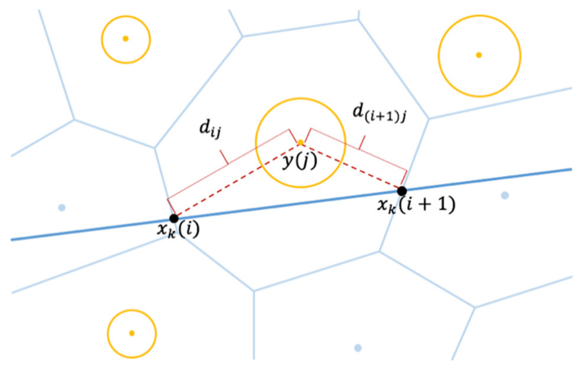
With these generated Voronoi cells, a distance from a route to each visited cell tower can be calculated from the points on its Voronoi boundaries that the route passes through. Figure 10 demonstrates an example where the points on visited cell tower’s Voronoi boundaries are marked with black solid circles. As shown in Figure 11, the distance between the route and each visited cell tower (or dij in Equation (2)) can be calculated in two ways: (1) the sum of distances from all passed points to the cell tower location i.e., dij + d(i+1)j; or (2) the minimum distance among all crossed points to the cell tower location i.e., d(i+1)j in this example. Note that in our study the Voronoi cells were generated using Matlab function called voronoi while another function called polyxpoly was used to find the intersection points between route and Voronoi cell boundaries.
2.4.4. Visited Voronoi Cell-Based Method
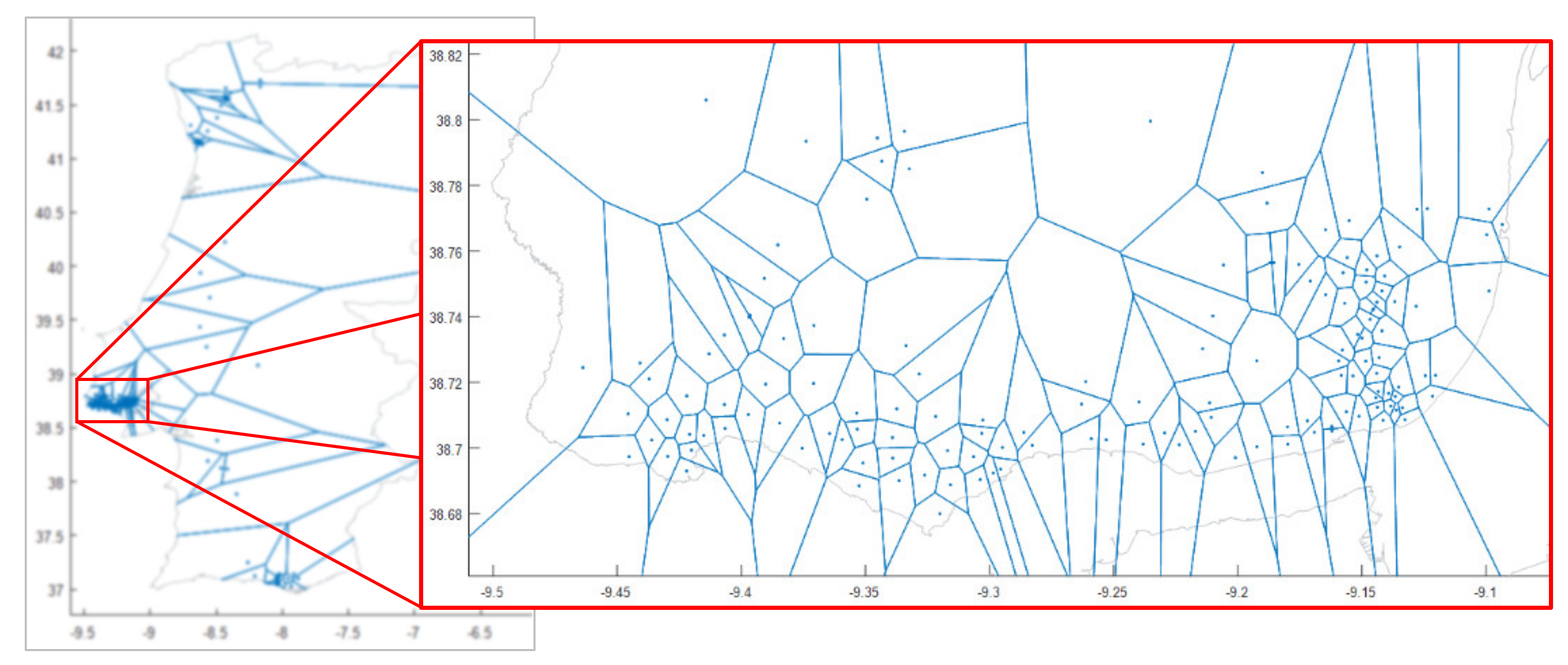
With the Voronoi-cells based method, potentially there may be some portions of the route that do not pass through visited Voronoi cells and hence are not considered in distance calculation. This can be addressed as we introduce another approach here where the key concept is to start with an individual subject’s Voronoi-cell map, which is individually generated by considering only the subject’s visited cell tower locations. This way, each of the route candidates will be passing through visited Voronoi cells along the way, so that the distance calculation is done over the whole route. Figure 12 shows an example of a sample subject’s visited Voronoi-cell map (with a zoom-in of the Lisbon area), which takes into account only the subject’s visited cell tower locations in generating the Voronoi cells. By using this approach, Figure 13 shows a sample subject’s (previously shown in Figure 10) route choices that pass through the visited Voronoi cells. The distance calculation between each route and visited cell towers can then be carried out as previously described in the Voronoi-cell based method (Section 2.4.3).
2.4.5. Noise Filtering
Although commuting trips constitute the majority of individual trips, there are also other trips made to/from elsewhere besides home and workplace. These non-commuting trips also are present in forms of logs of connectivity and can be reflected from the CDR data. Yet, as our focus is on commuting trips, the cellular network connectivity associated with these non-commuting journeys can be considered noise.
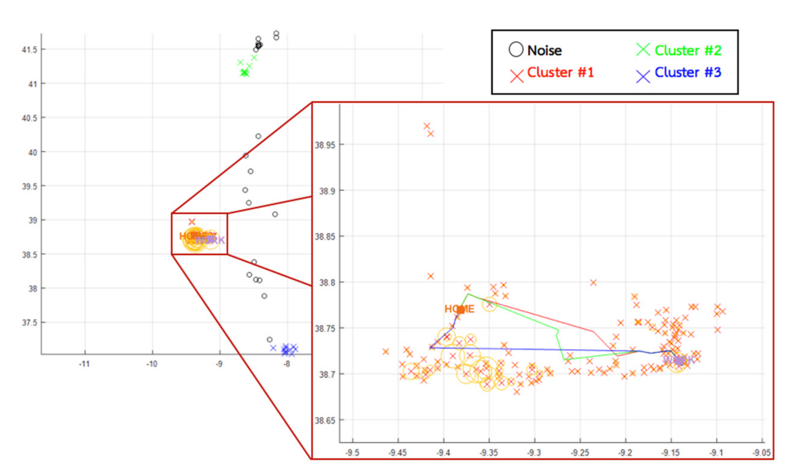
To reduce this noise from our commuting route choice inference, we introduce two approaches. First approach involves applying the DBSCAN algorithm [39], which is a density-based spatial clustering method that groups together data points with many nearby neighbors and filters out outliers that are data points lying alone in low-density regions. To proceed with the DBSCAN, there are two required parameters, which are the radius of a neighborhood (ε) and the minimum number of points required to form a dense region (minPts) for which we set ε to be equal to the commuting distance (i.e., direct distance between home and workplace) and minPts = 10, respectively. The values of these parameters were chosen and justified by our observations of the results based on which we believed that our chosen values were suitable. Different practical choices of DBSCAN parameters can of course be worth exploring in a future study. Choosing optimal choices of these two parameters is still an open research question as shown in a sensitivity analysis of spatiotemporal trajectory data clustering by Wong and Huang [40]. The two parameters apparently are against each other to a certain degree—i.e., increasing the value of minPts will disband larger clusters into smaller ones—while the value ε determines the spatial scale of cluster detection and hence increasing ε value produces extensive clusters. Appropriate values of these two parameters have been suggested in some studies [41,42], however these suggestions are not quite general as they are data dependent. In our case, the starting point is set to be the subject’s home cell tower location, so that the first cluster is a group of visited cell tower locations located near the commuting route. Therefore, only this first cluster is considered in our route choice inference while other clusters and noise are considered altogether as a noise and discarded. Figure 14 shows a clustering result of DBSCAN of a sample subject whose Cluster #1 is further considered in our route inference method while the rest of the visited cell towers is considered as noise and discarded.
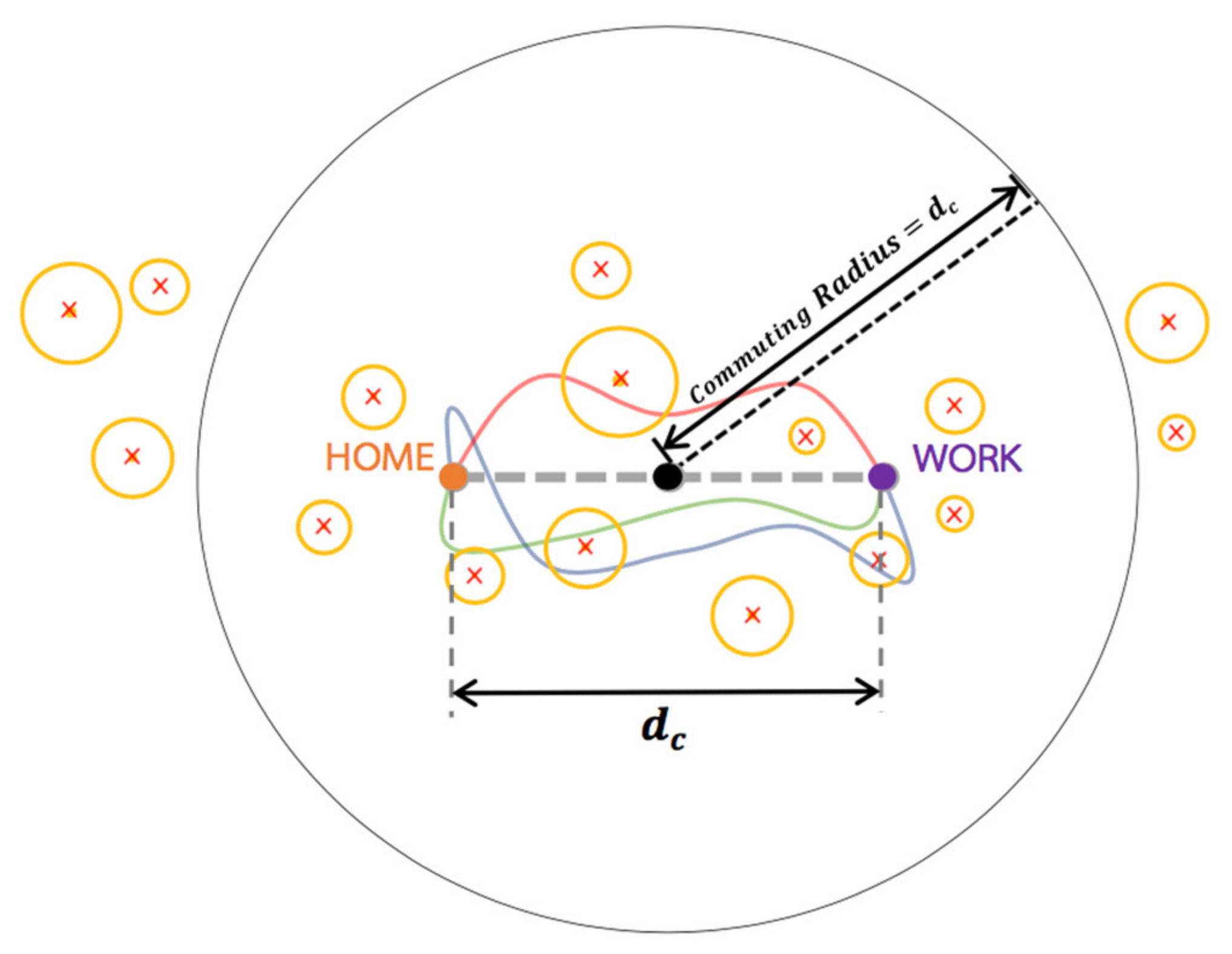
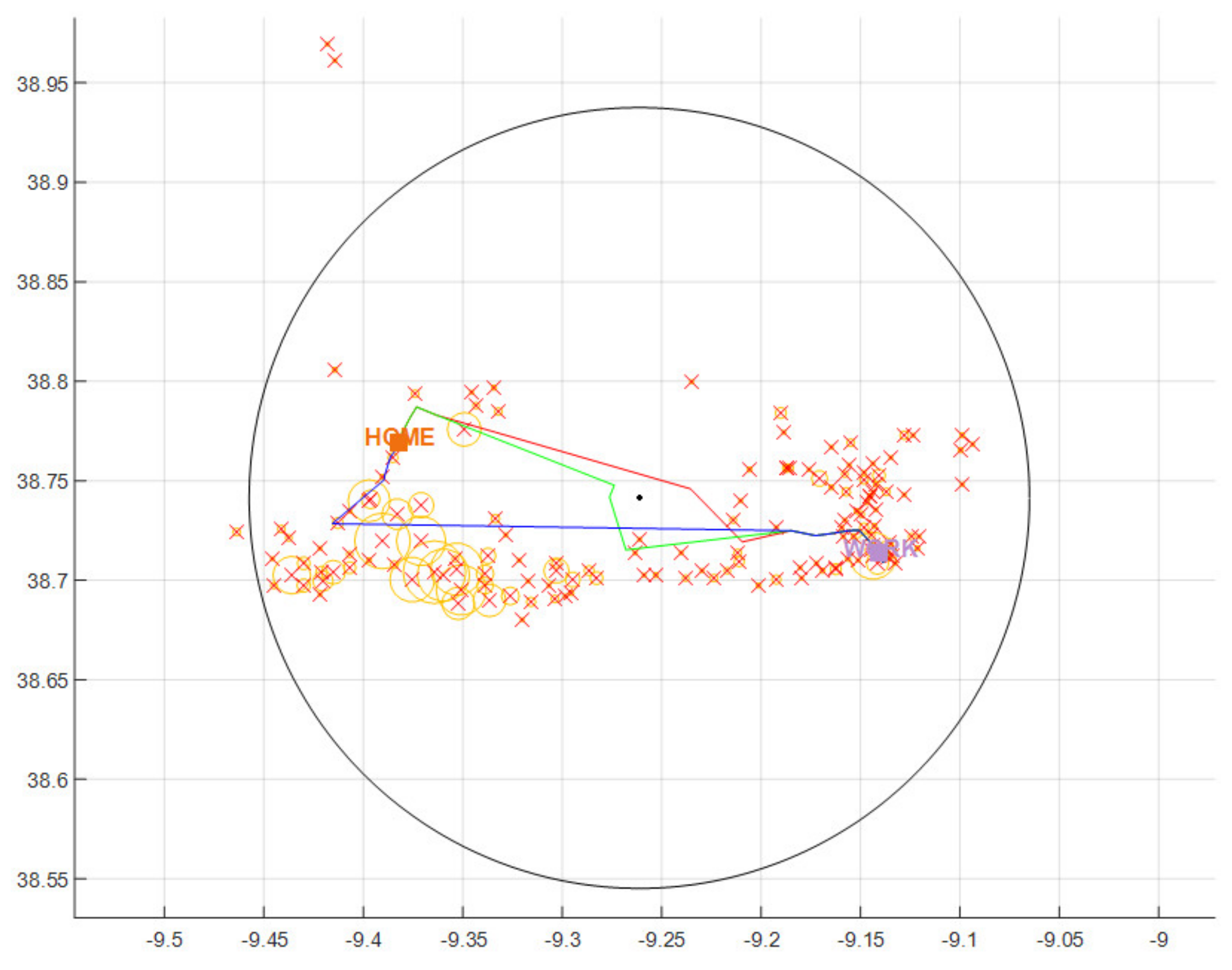
Our second approach to filtering out visited cell towers that are unlikely related to commuting trip, i.e., cell towers that are further away from the route choices, or considered as noise involves the use of commuting distance, i.e., direct home-workplace distance, which is used as ‘commuting radius’ to draw a noise filtering scope, as an analogy to bandpass filter. This noise filtering scope is centered at the midpoint on a straight line drawn between the home and workplace. All visited cell towers that are located within the scope of commuting radius are then further considered for our route inference while the rest is considered as noise and discarded. Figure 15 shows a graphic demonstrating this commuting-radius based noise filtering approach. For an actual example, Figure 16 shows a result of the commuting-radius based noise filtering (of the subject previously shown in Figure 14) where cell towers located within the enclosed commuting-radius scope are further taken otherwise discarded as noise.
3. Results
Here, we present the results of our route inference methods including the interpolation-based, shortest distance-based, Voronoi cell-based, and visited Voronoi cell-based methods implemented with and without noise filtering (DBSCAN and commuting radius-based). Accuracy rate was calculated by comparing the inferred route against a ground truth.
As obtaining the actual route choice information from the subjects was not possible, so we generated a ground true based on a visual inspection and hand labeling of data, which was believed to be most reasonably feasible in our case here. For consistency, one person was designated for the task and asked to hand label the route that was mostly believed to be the taken commuting route choice. The designated hand-labelling person viewed a subject’s CDR connectivity along with route choices (similar to the one shown in Figure 3) and was asked to identify the most probable route taken. The hand-labelling person was asked to only hand label the most probable route with high confidence, so the person did not hand label every examined subject but only those whose most probable route choices were clearly obvious to her. This exhaustive hand-labeling task yielded a 90-subject ground truth for our experiment.
3.1. Interpolation-Based Methods
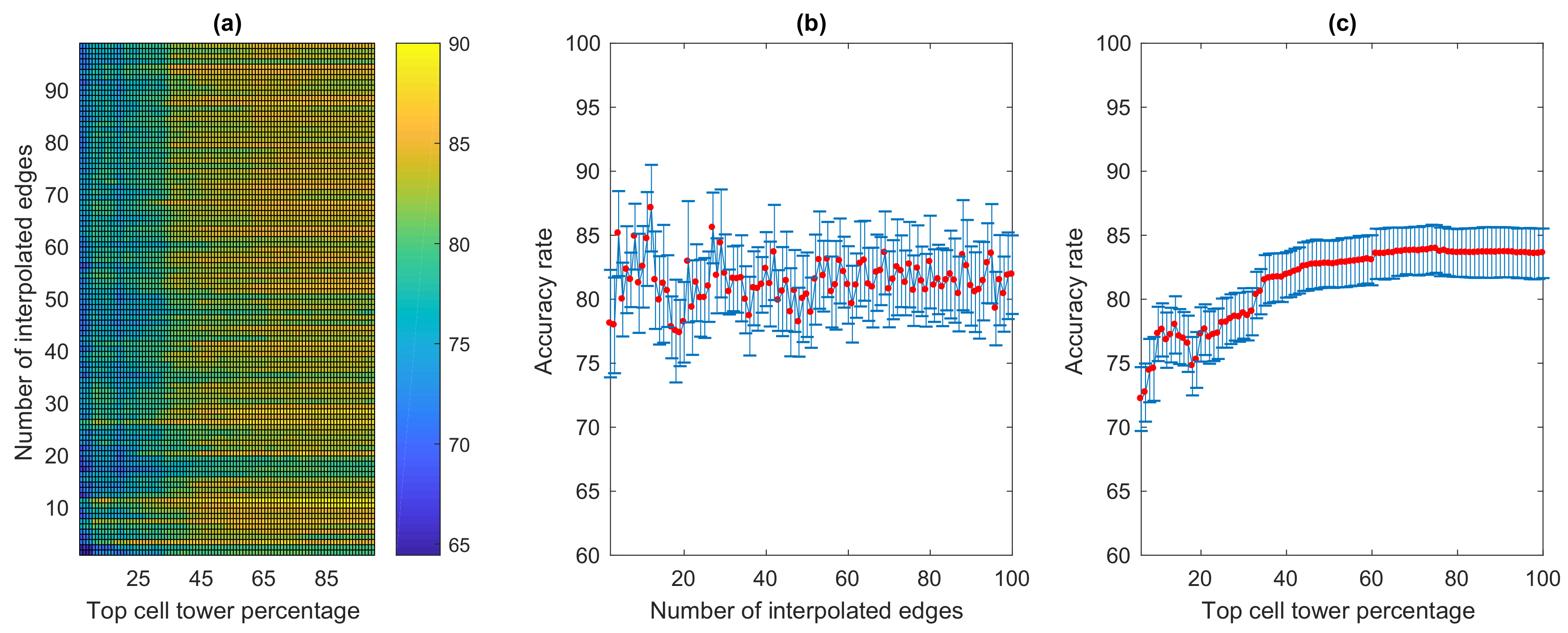
For the interpolation-based method, an accuracy rate was calculated for each of the varying number of interpolated edges ranging from 2 to 100 edges to observe the impact of the level of interpolation. Furthermore, the used (visited) cell towers were ranked from the most to the least used towers, for which an accuracy rate was calculated from the top 1% to 100% (all) used cell towers.
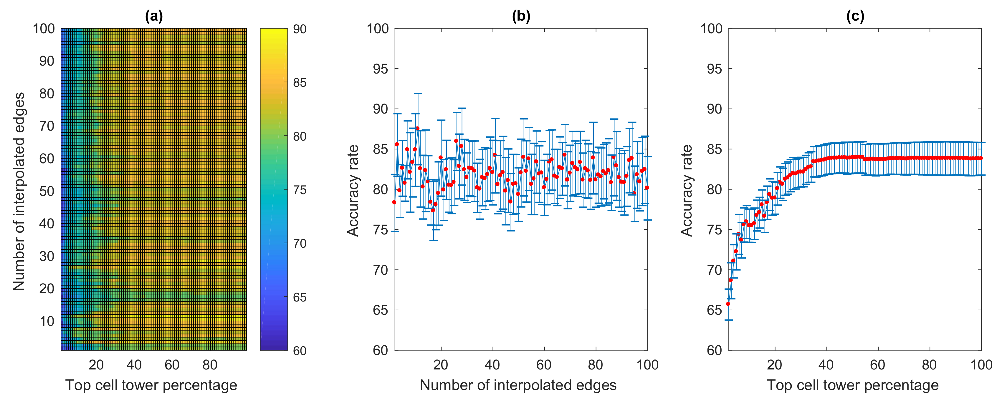
Overall result is shown in Figure 17a for a total of 99 × 100 = 9900 experimental setups for which accuracy rates were calculated. The overall average accuracy rate is 82.05%. The accuracy reaches its maximum of 90% for 62 times which all happen when the number of interpolated edges is set to 12 edges and the top cell tower percentage varies from 34% to 95%. Figure 17b shows the average accuracy rates of each of the varying number of interpolated edges along with corresponding standard deviation bars, which confirms that with 12 interpolated edges, the average accuracy rate is at the highest of 87.72%, averaged across all top cell tower percentage variations. Interestingly, when considering the average accuracy rates across all top cell tower percentages as shown in Figure 17c, the average accuracy gradually rises and becomes stable as the number of top cell towers considered for accuracy rate calculation increases. The average accuracy rate rises to 83.04% at 26% top cell towers and does not change much as it continues to slightly climb up to 83.79% when it reaches all 100% top cell towers. This suggests that only some percentage of top visited cell towers can be sufficient for the route choice inference, as it does not significantly improve the accuracy by taking more data presumably less relevant. This result opens up an interesting research question of how much of the individual CDR data that is said to be significantly sufficient and relevant to the route choice inference, which is worth future investigation.
For the interpolation-based method implemented with the DBSCAN-based noise filtering, the examined number of interpolated edges varies from 2 to 100 edges, while the percentage of top cell towers ranges from 2% to 100% in this experiment (as there were not top cell towers in some cases made up by 1% after some towers being filtered out as noise). The overall result from a total of 99 × 99 = 9801 experimental setups is shown in Figure 18a. The overall average accuracy is 81.85%, while the highest accuracy rate is 90% when the number of interpolated edges is 12 and the percentage of top cell towers is from 37% to 95%. Along the same line, Figure 18b shows at the highest average accuracy rate of 87.49% is reached when 12 interpolated edges were used. Our examination of top cell tower percentages in Figure 18c shows that with DBSCAN, the average accuracy rate increases slightly slower than the interpolation-based method without DBSCAN to reach its stable level. In this experiment, it reaches a stable level (83.41% accuracy) at 35% of top cell towers, which is slower than that of the normal method whose stable accuracy rate is reached at 26% of top cell towers. The average accuracy once reaches its stable level at 83.41%, it continues to slowly rise to 83.79% when the entire cell towers were considered.
Lastly, with the commuting radius-based noise filtering, the interpolation-based method preforms slightly worse than the previous two methods. The variation of examined number interpolated edges is the same as in previous experiments which is 2–100 edges, but the percentage of top cell towers in this experiment varies from 6% to 100%. The overall result obtained from a total of 99 × 96 = 9504 experimental setups is shown in Figure 19a where the overall average accuracy rate is 81.35%. The highest accuracy is 90%, which happen when the number interpolated edges is 12 and percentage of top cell towers is from 59% to 93%. From the perspective of the number interpolated edges, the average accuracy reaches its maximum at 84.70% with 12 edges, as shown in Figure 19b. With the varying percentage of top cell towers, the accuracy reaches its stable rate at 83.03% when the top 58% cell towers were considered, and it moves up and down slightly and eventually stands at 83.59% when the entire visited cell towers were taken into consideration (Figure 19c).
3.2. Shortest Distance-Based Methods
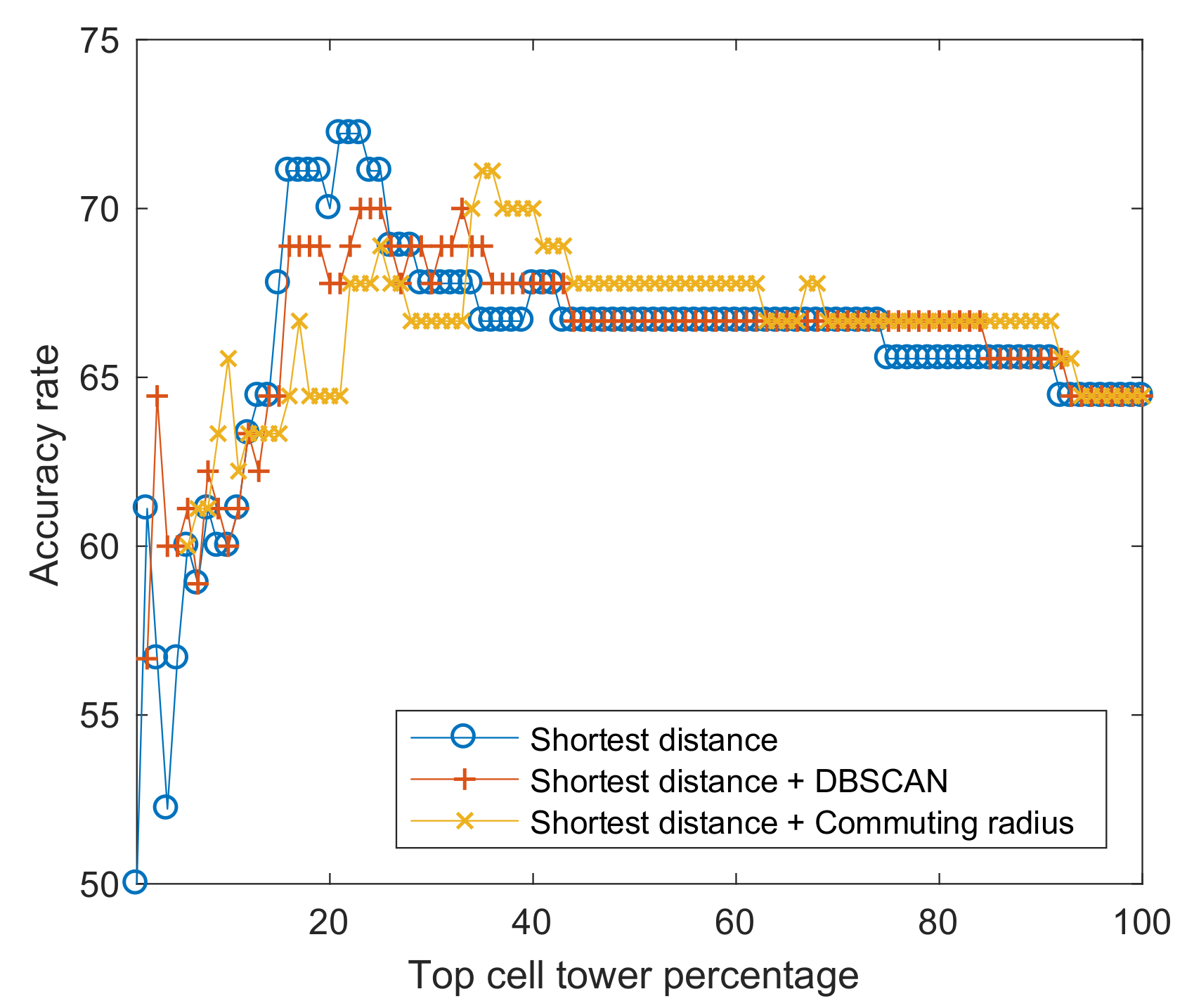
With the shortest distance-based method, an accuracy rate was calculated for each varying percentage of top cell towers implemented with and without noise filtering. All results from three different models are shown in Figure 20, including the shortest distance-based method without noise filtering (Shortest distance), the shortest distance-based method with DBSCAN (Shortest distance + DBSCAN), and the shortest distance-based method with commuting radius-based noise filtering (Shortest distance + Commuting radius). The top cell tower percentage varies from 1–100% for the Shortest distance method, from 2–100% for the Shortest distance + DBSCAN method, and from 6–100% for the Shortest distance + Commuting radius method.
With the Shortest distance method, its accuracy rate has an uprising trend and reaches the maximum value of 72.22% when the top cell lower percentage is 21%, 22%, and 23%. It then shows a continuous dropping trend to reach 64.44% accuracy rate when the entire (100%) visited cell towers were taken into account. The result of the Shortest distance + DBSCAN method shows a similar up-and-down trend with the Shortest distance method. It rises to reach its maximum at 70% when the top cell tower percentage is 23%, 24%, and 33%, then gradually drops to eventually reach 64.44% when the entire cell towers were considered. Lastly, the resulting accuracy rates of the Shortest distance + Commuting radius method also appear to a similar trend where it rises to its maximum value of 71.11% when 35% or 36% top cell towers were considered. It then slowly decreases to eventually reach 64.44%. Overall, the shortest distance-based method without noise filtering appears to have a better performance than implementing it with a noise filtering, as it shows to be the fastest to reach its maximum accuracy rate, and it also poses the highest accuracy value among all three examined methods.
3.3. Voronoi Cell-Based Methods
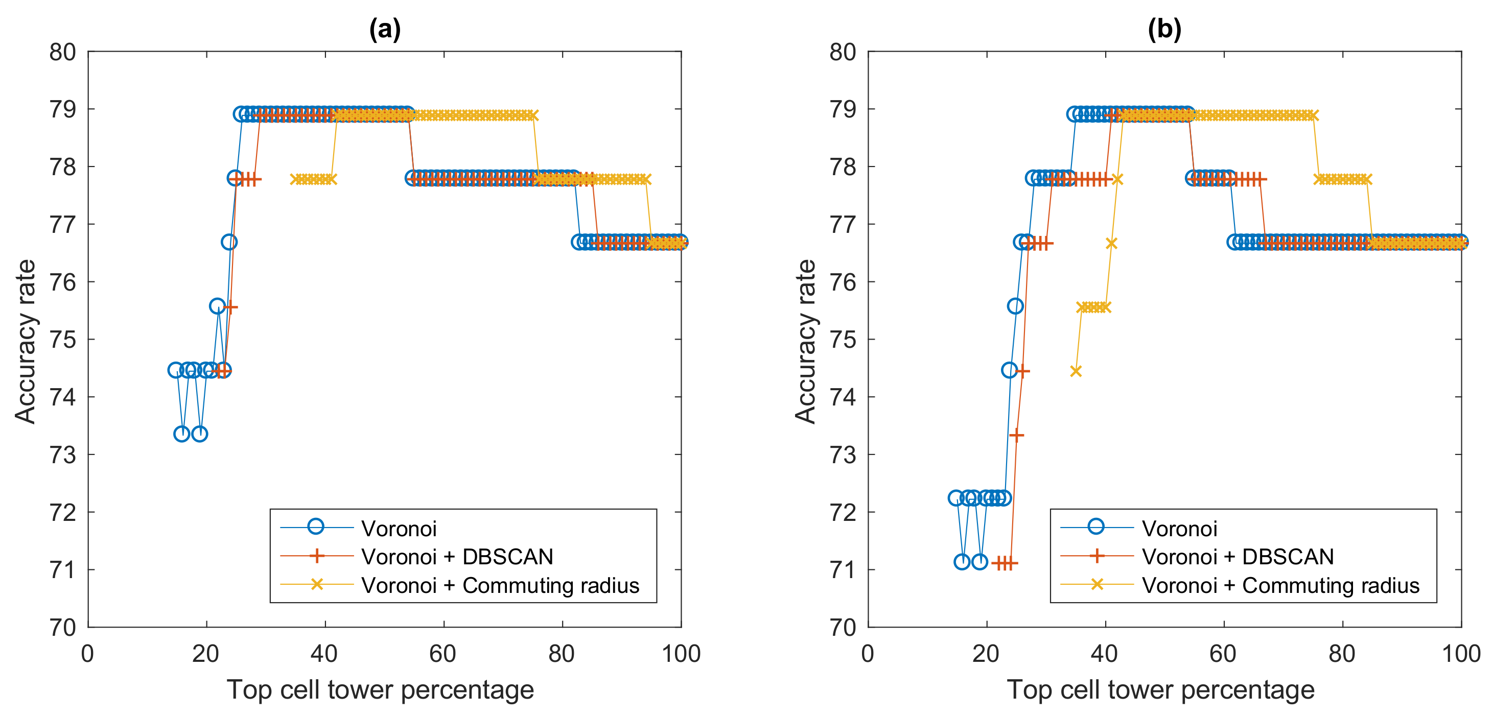
The Voronoi cell-based method was implemented with and without noise filtering. The results are shown in Figure 21. Percentage of top cell towers considered for the route inference varies and starts from 15%, 22%, and 35% for the Voronoi cell-based method without noise filtering (Voronoi), with DBSCAN (Voronoi + DBSCAN), and with commuting radius-based noise filtering (Voronoi + Commuting radius), respectively. The top cell tower percentage starts from a different value in each of the three methods due to the obtainable amount of top cell towers with a specified percentage value. Two separated set of experiments were implemented, one with the summed distance approach and the other with the shortest distance approach, as described in Section 2.4.3—i.e., distance measured from passed points to a visited cell tower location (dij, d(i+1)j to y(j)).
For the summed distance approach as shown in Figure 21a, the Voronoi method shows an uprising trend to reach its maximum accuracy of 78.89% with top 26% cell towers and remains at this accuracy until the top 54% cell towers considered, then it drops slightly to 77.78% and remains there from top 55–82% cell towers and then takes another step drop to 76.67% and lasts for the rest of the cell tower percentages. The Voronoi + DBSCAN method exhibits a similar result with the Voronoi method, as its accuracy rate climbs up in the same fashion but reaches the same maximum rate (78.89%) later at top 29% cell towers and remains at the level before it drops to 77.78% at the same 55% top cell tower level but remains there until 85% top cells before taking the last step drop to the same accuracy rate of 76.67% for the rest of the way. The three-step accuracy rates are also observed for the Voronoi + Commuting radius method, as it rises to the maximum (78.89%) and remains there from 42% to 75% top cells, and then later down steps are 76–94% and 95–100%. These stepwise accuracy rates are most possibly due to the issue previously discussed in Section 2.4.3 that with the Voronoi-cells based method, there may potentially be some portions of the route that do not pass through visited Voronoi cells and hence they are not considered in distance calculation. A chunk of top cell towers are likely required to make an impact on accuracy rate, thereby a stepwise accuracy result is observed.
For the Voronoi-based shortest distance approach, the result is shown in Figure 21b where the top cell tower percentage starts at 15%, 22%, and 35% for the Voronoi cell-based method without noise filtering (Voronoi cells), with DBSCAN (Voronoi + DBSCAN), and with commuting radius-based noise filtering (Voronoi + Commuting radius), respectively. Stepwise accuracy results are also observed here. The calculated accuracy rates of all three models exhibit a similar trend, as they all rise to reach the same maximum rate of 78.89% and remain there for some top cell tower percentages, then drops to 77.78% and later 76.67%. The Voronoi method reaches the maximum with the least percentage of top cell towers of 35%, followed by the Voronoi + DBSCAN of 41% and then Voronoi + Commuting radius of 43%. The Voronoi + Commuting radius, however, is able to stay at the maximum rate for the largest portion of the top cell percentages, i.e., 43–75%.
3.4. Visited Voronoi Cell-Based Methods
Likewise, the visited Voronoi cell-based method (V-Voronoi) was implemented without and with noise filtering (V-Voronoi + DBSCAN and V-Voronoi + Commuting radius), as well as altered with the summed distance and shortest distance approaches. The top cell percentage starts at 11%, 12%, and 39% for V-Voronoi, V-Voronoi + DBSCAN, and V-Voronoi + Commuting radius, respectively. The results are shown in Figure 22.
With the summed distance approach, the maximum accuracy among three methods of 75.56% was achieved by the V-Voronoi + Commuting radius at 42% top cell tower level, followed by the V-Voronoi at 73.33% when top cell percentage is in the ranges 25–28% and 36–49%, and the V-Voronoi + DBSCAN at also 73.33% for a span of 40–56% top cell towers. With the shortest distance approach, the maximum accuracy among all three methods was 74.44%, which was achieved by V-Voronoi + DBSCAN for 45–47% top cell towers and V-Voronoi + Commuting radius for 64–69% top cell towers.
Interestingly, the performance of the visited Voronoi cell-based methods are lower than that of the Voronoi cell-based methods. This may be due to the consideration of only visited Voronoi cells that draws up larger coverage zones (or cells), which may negatively affect the distance calculation.
3.5. Result Summary
The results from all sets of experiment of our developed and examined methods for route choice inference including the interpolation-based, shortest distance-based, Voronoi cell-based, and visited Voronoi cell-based methods, implemented with and without DBSCAN or commuting radius-based noise filtering are summarized in Table 1.
Interestingly, the interpolation-based method has the best result in both points of view of the maximum and average accuracy rates. From the average accuracy rate’s perspective, the top five rankings are Interpolation (82.05%), Interpolation + DBSCAN (81.85%), Interpolation + Commuting radius (81.35%), V-Voronoi cells (summed dist.) + Commuting radius (77.88%), and then Voronoi cells (shortest dist.) + Commuting radius (77.83%). The bottom five rankings include Shortest distance (65.89%), Shortest distance + DBSCAN (66.20%), Shortest distance + Commuting radius (66.61%), V-Voronoi cells (shortest dist.) (70.12%), and V-Voronoi cells (shortest dist.) + DBSCAN (70.46%). If grouped by the main method, the interpolation-based group has the highest average accuracy rate (81.75%), followed by the Voronoi cells (summed dist.) group (77.54%), and Voronoi cells (shortest dist.) group (77.25%).
From the point of view of a receiver operating characteristic curve, or ROC curve, which is a performance measurement for classification problem at various thresholds settings, the performance across all route inference models with varying top cell percentages is in line with the results observed in Table 1 as all interpolation-based models are among the top performance on the ROC curve, as shown in Figure 23. Model performance is measured in forms of true positive rate (TPR) or sensitivity versus false positive rate (FPR) or probability of false alarm.
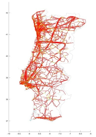
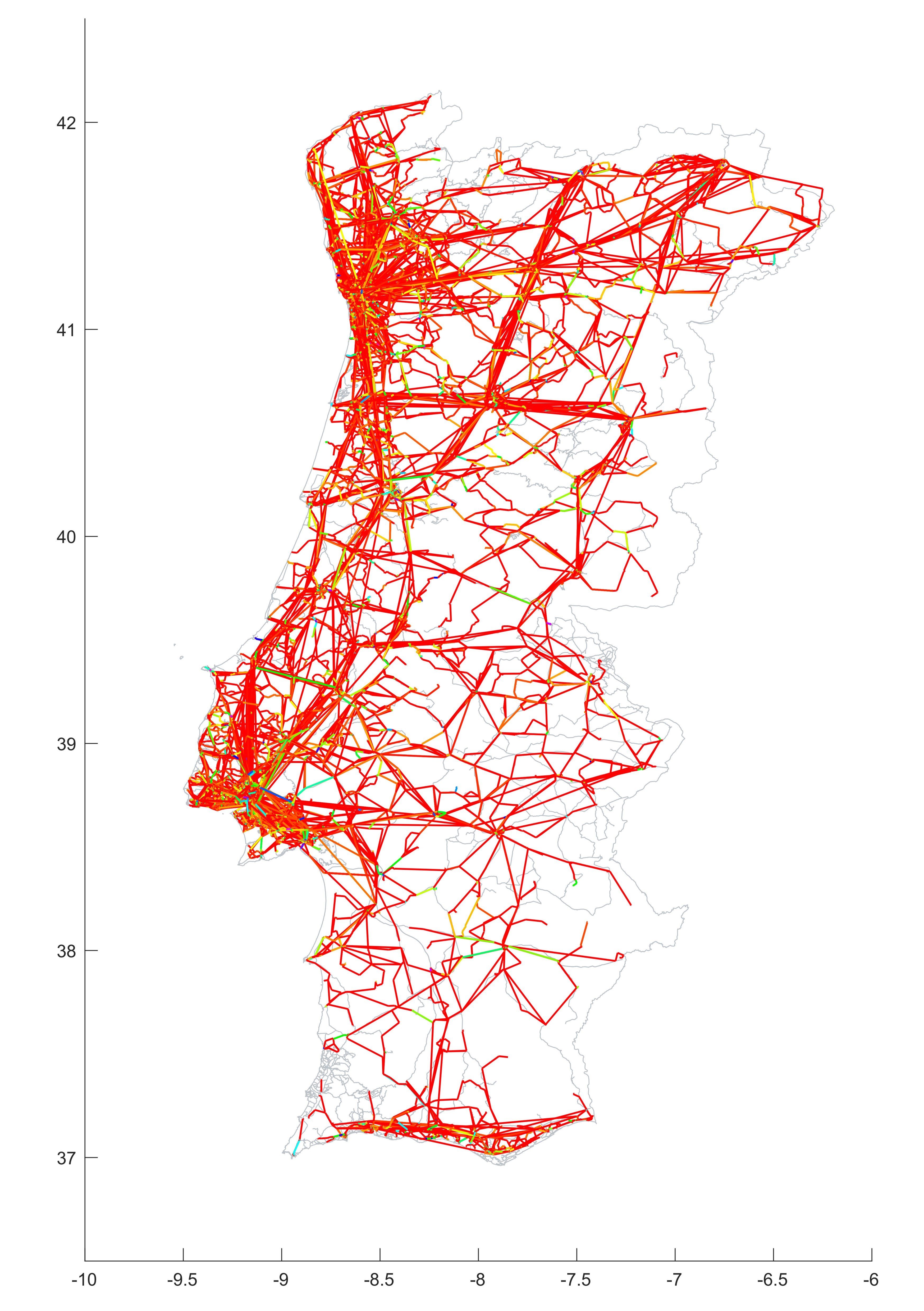
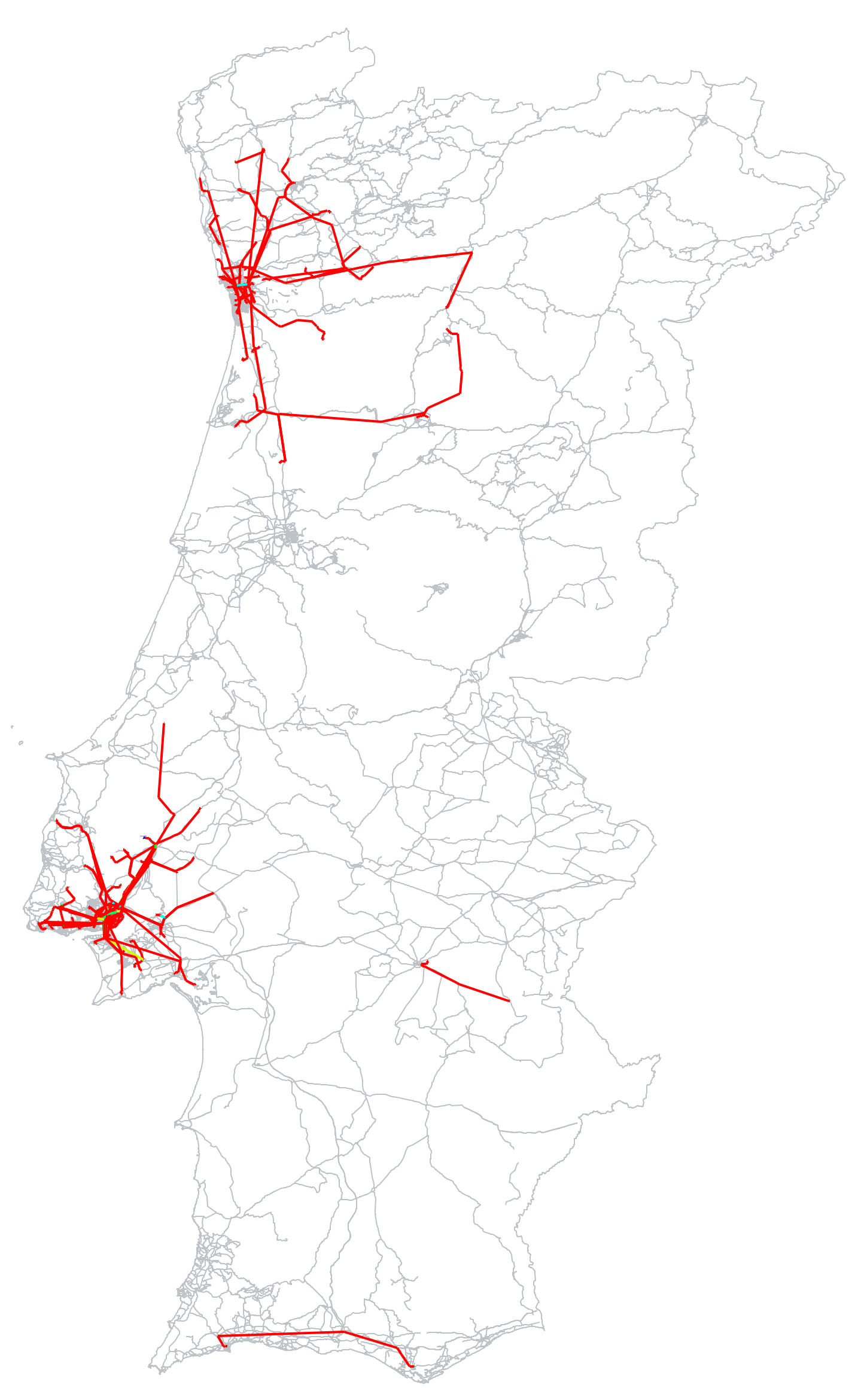
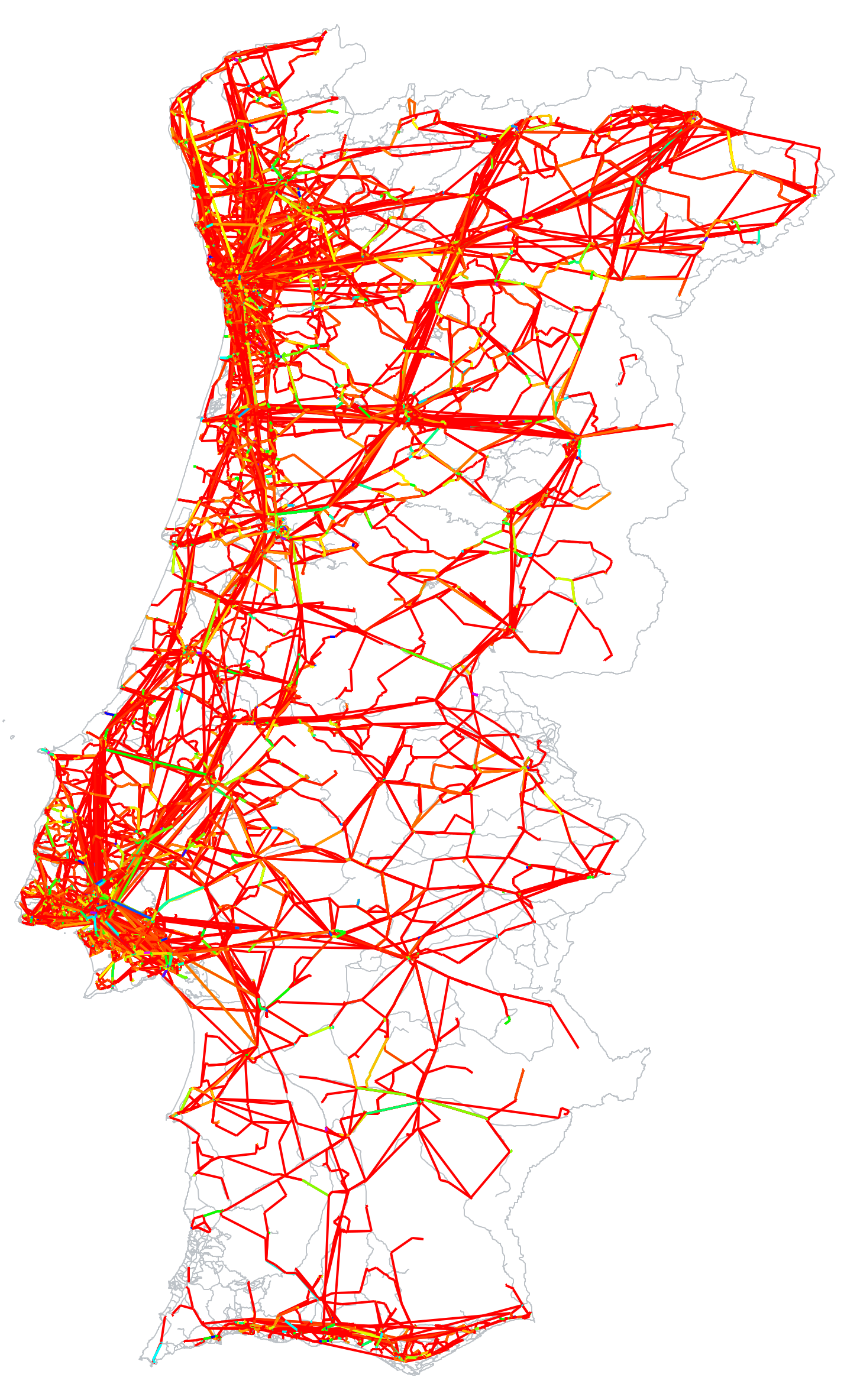
As our ultimate goal of this investigation is to offer a new and more efficient way than the traditional surveys to gather a route choice information at a large scale, so we applied our best method (i.e., interpolation-based with 12 edges) to infer commuting route choices in Portugal. Our ground truth of 90 subjects’ route choices is shown in Figure 24, and the inferred route choices of 110,213 subjects on the Portugal road network shown in Figure 25. With our approach, commuting route choice information can be gathered at anytime, which is intuitive and more up-to-date compared to the travel survey that is collected once every 5–10 years. Thus, transportation can be better informed, planned, and designed to meet the current traffic demand and travel behavior.
4. Conclusions
Its ubiquity has turned mobile phone into personal sensor that collects digital traces of individual through the usage of provided services, such as voice calls, messages, and internet. These communication logs are collected purposely for billing, but collectively on a large scale these individual traces can be regarded as a valuable behavioral data source from which insights into human behavior can be gained. This study makes use of the location traces of mobile phone users to gather information on route choices of individuals in their commuting trips. This offers a better alternative to the traditional travel surveys such as roadside interviews and questionnaires, which are costly and time-consuming. A total of 18 different route choice inference models have been developed and examined. Our route choice inference has been formulated as a problem of choosing the most probable route taken among different route choice candidates based on the location traces of individual mobile phone’s connectivity i.e., connected (or visited) cellular towers. Four main models are based on the interpolation of route waypoints for calculating distance between a probable route choice and connected cell towers, the shortest distance between a route choice with original waypoints and visited cellular towers, the Voronoi cells that assign a route choice into multiple coverage zones, and the consideration of only visited Voronoi cells that assign a route choice into individual coverage zones. For both Voronoi-based models, two variations in calculating the distance have also been implemented; one with the summed distance of passed points and the other approach is the use of only the shortest distance of all passed points on each considered Voronoi boundaries. Each of these models has been implemented with and without noise filtering, which includes applying the DBSCAN algorithm and our own approach that uses commuting distance to draw a noise filtering scope, as an analogy to bandpass filter. Our model development and experiment were carried out using a mobile network phone dataset (or CDR) from Portugal. As the result, from the accuracy rate’s point of view, the interpolation-based models have the best performance followed by the consideration of only visited Voronoi cell-based model with summed distance approach and with commuting radius-based noise filtering, and then the Voronoi cell-based shortest distance approach and with commuting radius-based noise filtering.
Interestingly, reflecting on our experimental results seems to suggest that the noise may not be noise as initially perceived after all. Consideration of the entire data tends to produce a better performance than the noise filtered data. Relevance is probably the key here as evidenced in the top cellular tower percentage experiments that with some portion of top cell towers the model performs better than taking the entire data in consideration, as we varied the percentage of top (used/visited) cellular towers in our accuracy calculation.
From a small ground truth set, commuting route choices of people in Portugal are inferred and demonstrated on the road network as a case study. Our developed and examined models can have an immediate implication in gathering route choice information on a large scale that facilitates the four-step model in transportation forecasting. Our models and approaches can also serve as a baseline for future development and investigation into the route choice inference problem which is based on solely on CDR data, as they provide a perspective to both problem formation and solution.
Nonetheless, there are a number of significant limitations to our study. The first of these is the possibility of multiple route choices. Our assumption in this study was that a person takes only one route choice for commuting, which is not always the case for everyone but presumably for most people. Another potential limitation is an arguably small set of ground truth, which is due to the exhaustive nature of our hand labeling task. A larger ground truth size may potentially increase the significance to the model evaluation. A third limitation relates to the route choice candidates gathered via the Google Maps Directions API, which may not precisely be the route choices available. Yet, we believe that the gathered route choices still share many similarities with the actual ones as the suggested route choices are fundamentally based on the fastest travel time, which is presumably the approach of most commuters. As our analysis was performed based on mobile phone users in Portugal, a final limitation is about the extent to which our findings are applicable beyond the country of case study. Though it is a case study to demonstrate our model development and analysis, we strongly believe that the findings are still valid to a large extent and likely to be applicable to countries with broadly similar social, cultural, and economic profiles with Portugal, which is a member of the 26 Schengen countries and a developed country that shares significant similarities with several European and other developed counties in the world.
As for future research directions, this study opens up a number of interesting related research questions worth exploring in a future study, such as how to determine a percentage of top visited cell towers that is effectively adequate for route choice inference. Especially, in the big data era, data streams consist of both relevant and irrelevant portions. How to effectively extract only relevant ones is the key. Another future research trajectory is utilizing the temporal context of the CDR data in route choice inference, which is left out of the present study. Consideration of temporal sequences could potentially improve the model’s performance. Lastly, the reasoning behind chosen route choices is another interesting aspect for investigation, which could be related to connectivity of road network and how it is designed.
Author Contributions
Conceptualization, Santi Phithakkitnukoon and Carlo Ratti; Methodology, Pitchaya Sakamanee and Santi Phithakkitnukoon; Validation, Santi Phithakkitnukoon and Zbigniew Smoreda; Formal Analysis, Pitchaya Sakamanee andZbigniew Smoreda; Investigation, Pitchaya Sakamanee and Santi Phithakkitnukoon; Resources, Zbigniew Smoreda; Data Curation, Pitchaya Sakamanee and Santi Phithakkitnukoon; Writing—Original Draft Preparation, Pitchaya Sakamanee and Santi Phithakkitnukoon; Writing—Review and Editing, Santi Phithakkitnukoon, Zbigniew Smoreda, and Carlo Ratti; Supervision, Santi Phithakkitnukoon; Project Administration, Santi Phithakkitnukoon; Funding Acquisition, Santi Phithakkitnukoon All authors have read and agreed to the published version of the~manuscript.
Funding
This research was funded by the Thailand Research Fund, grant number RSA6180014.
Conflicts of Interest
The authors declare no conflict of interest.
References
- Vickrey, W. Congestion Theory and Transport Investment. Am. Econ. Rev. 1969, 59, 251–260. [Google Scholar]
- Mcnally, M.G. The Four Step Model. Handb. Transp. Model. 2007, 1, 35–53. [Google Scholar]
- Stopher, P.R.; Greaves, S.P. Household travel surveys: Where are we going? Transp. Res. Part A Policy Pract. 2007, 41, 367–381. [Google Scholar] [CrossRef]
- Shen, L.; Stopher, P.R. Review of GPS Travel Survey and GPS Data-Processing Methods. Transp. Rev. 2014, 34, 316–334. [Google Scholar] [CrossRef]
- Van Alsenoy, B. General Data Protection Regulation. In Data Protection Law in the EU: Roles, Responsibilities and Liability, 1st ed.; KU Leuven Centre for IT & IP Law Series; Intersentia: Cambridge, UK, 2019. [Google Scholar]
- Cuttone, A.; Lehmann, S.; González, M.C. Understanding predictability and exploration in human mobility. EPJ Data Sci. 2018. [Google Scholar] [CrossRef] [Green Version]
- Rupi, F.; Poliziani, C.; Schweizer, J. Data-driven Bicycle Network Analysis Based on Traditional Counting Methods and GPS Traces from Smartphone. ISPRS Int. J. Geo-Inf. 2019, 8, 322. [Google Scholar] [CrossRef] [Green Version]
- Phithakkitnukoon, S.; Horanont, T.; Witayangkurn, A.; Siri, R.; Sekimoto, Y.; Shibasaki, R. Understanding tourist behavior using large-scale mobile sensing approach: A case study of mobile phone users in Japan. Pervasive Mob. Comput. 2015, 18, 18–39. [Google Scholar] [CrossRef]
- Caceres, N.; Wideberg, J.P.; Benitez, F.G. Review of traffic data estimations extracted from cellular networks. IET Intell. Transp. Syst. 2008, 2, 179–192. [Google Scholar] [CrossRef]
- Blondel, V.D.; Decuyper, A.; Krings, G. A survey of results on mobile phone datasets analysis. EPJ Data Sci. 2015. [Google Scholar] [CrossRef] [Green Version]
- De Montjoye, Y.A.; Hidalgo, C.A.; Verleysen, M.; Blondel, V.D. Unique in the Crowd: The privacy bounds of human mobility. Sci. Rep. 2013, 3, 1376. [Google Scholar] [CrossRef] [Green Version]
- Shi, F.; Zhu, L. Analysis of trip generation rates in residential commuting based on mobile phone signaling data. J. Transp. Land Use 2019, 12, 201–220. [Google Scholar] [CrossRef]
- Bwambale, A.; Choudhury, C.F.; Hess, S. Modelling trip generation using mobile phone data: A latent demographics approach. J. Transp. Geogr. 2019, 76, 276–286. [Google Scholar] [CrossRef] [Green Version]
- Di Donna, S.A.; Cantelmo, G.; Viti, F. A Markov chain dynamic model for trip generation and distribution based on CDR. In Proceedings of the International Conference on Models and Technologies for Intelligent Transportation Systems, Budapest, Hungary, 3–5 June 2015; pp. 243–250. [Google Scholar]
- Bonnel, P.; Hombourger, E.; Olteanu-Raimond, A.M.; Smoreda, Z. Passive mobile phone dataset to construct origin-destination matrix: Potentials and limitations. Transp. Res. Procedia 2015, 11, 381–398. [Google Scholar] [CrossRef]
- Demissie, M.G.; Phithakkitnukoon, S.; Sukhvibul, T.; Antunes, F.; Gomes, R.; Bento, C. Inferring Passenger Travel Demand to Improve Urban Mobility in Developing Countries Using Cell Phone Data: A Case Study of Senegal. IEEE Trans. Intell. Transp. Syst. 2016, 17, 2466–2478. [Google Scholar] [CrossRef]
- Wu, H.; Liu, L.; Yu, Y.; Peng, Z.; Jiao, H.; Niu, Q. An Agent-based Model Simulation of Human Mobility Based on Mobile Phone Data: How commuting relates to congestion. ISPRS Int. J. Geo-Inf. 2019, 8, 313. [Google Scholar] [CrossRef] [Green Version]
- Mamei, M.; Bicocchi, N.; Lippi, M.; Mariani, S.; Zambonelli, F. Evaluating origin–destination matrices obtained from CDR data. Sensors (Switz.) 2019, 19, 4470. [Google Scholar] [CrossRef] [Green Version]
- Hankaew, S.; Phithakkitnukoon, S.; Demissie, M.G.; Kattan, L.; Smoreda, Z.; Ratti, C. Inferring and Modeling Migration Flows Using Mobile Phone Network Data. IEEE Access 2019, 7, 164746–164758. [Google Scholar] [CrossRef]
- Demissie, M.G.; Phithakkitnukoon, S.; Kattan, L. Understanding Human Mobility Patterns in a Developing Country Using Mobile Phone Data. Data Sci. J. 2019, 18, 1–13. [Google Scholar] [CrossRef] [Green Version]
- Demissie, M.G.; Phithakkitnukoon, S.; Kattan, L. Trip Distribution Modeling Using Mobile Phone Data: Emphasis on Intra-Zonal Trips. IEEE Trans. Intell. Transp. Syst. 2018, 20, 2605–2617. [Google Scholar] [CrossRef]
- Phithakkitnukoon, S.; Sukhvibul, T.; Demissie, M.; Smoreda, Z.; Natwichai, J.; Bento, C. Inferring social influence in transport mode choice using mobile phone data. EPJ Data Sci. 2017, 6. [Google Scholar] [CrossRef] [Green Version]
- Wang, H.; Calabrese, F.; di Lorenzo, G.; Ratti, C. Transportation mode inference from anonymized and aggregated mobile phone call detail records. In Proceedings of the 13th International IEEE Conference on Intelligent Transportation Systems, Proceedings (ITSC), Funchal, Portugal, 19–22 September 2010. [Google Scholar]
- Graells-Garrido, E.; Caro, D.; Parra, D. Inferring modes of transportation using mobile phone data. EPJ Data Sci. 2018, 7. [Google Scholar] [CrossRef]
- Tettamanti, T.; Demeter, H.; Varga, I. Route choice estimation based on cellular signaling data. Acta Polytech. Hung. 2012, 9, 207–220. [Google Scholar]
- Breyer, N.; Gundlegård, D.; Rydergren, C. Cellpath Routing and Route Traffic Flow Estimation Based on Cellular Network Data. J. Urban Technol. 2018, 25, 85–104. [Google Scholar] [CrossRef]
- Bwambale, A.; Choudhury, C.; Hess, S. Modelling long-distance route choice using mobile phone call detail record data: A case study of Senegal. Transp. A Transp. Sci. 2019, 15, 1543–1568. [Google Scholar] [CrossRef]
- Yang, X.; Fang, Z.; Yin, L.; Li, J.; Zhou, Y.; Lu, S. Understanding the spatial structure of urban commuting using mobile phone location data: A case study of Shenzhen, China. Sustainability 2018, 10, 1435. [Google Scholar] [CrossRef] [Green Version]
- Jundee, T.; Kunyadoi, C.; Apavatjrut, A.; Phithakkitnukoon, S.; Smoreda, Z. Inferring commuting flows using CDR data: A case study of Lisbon, Portugal. In Proceedings of the UbiComp/ISWC 2018 - Adjunct Proceedings of the 2018 ACM International Joint Conference on Pervasive and Ubiquitous Computing and Proceedings of the 2018 ACM International Symposium on Wearable Computers, Singapore, 8–12 October 2018; pp. 1041–1050. [Google Scholar]
- Zagatti, G.A.; Gonzalez, M.; Avner, P.; Lozano-Gracia, N.; Brooks, C.J.; Albert, M.; Gray, J.; Antos, S.E.; Burci, P.; Erbach-Schoenberg, E.; et al. A trip to work: Estimation of origin and destination of commuting patterns in the main metropolitan regions of Haiti using CDR. Dev. Eng. 2018, 3, 133–165. [Google Scholar] [CrossRef]
- Phithakkitnukoon, S.; Smoreda, Z.; Olivier, P. Socio-geography of human mobility: A study using longitudinal mobile phone data. PLoS ONE 2012. [Google Scholar] [CrossRef] [Green Version]
- Horanont, T.; Phiboonbanakit, T.; Phithakkitnukoon, S. Resembling population density distribution with massive mobile phone data. Data Sci. J. 2018, 17, 1–9. [Google Scholar] [CrossRef] [Green Version]
- Chia, W.C.; Yeong, L.S.; Jia, F.; Lee, X.; Inn, S. Trip Planning Route Optimization with Operating Hour and Duration of Stay Constraints. In Proceedings of the 2016 11th International Conference on Computer Science & Education (ICCSE), Nagoya, Japan, 23–25 August 2016; pp. 395–400. [Google Scholar]
- Chou, Y.T.; Hsia, S.Y.; Lan, C.H. A hybrid approach on multi-objective route planning and assignment optimization for urban lorry transportation. In Proceedings of the 2017 International Conference on Applied System Innovation (ICASI), Sapporo, Japan, 13–17 May 2017; pp. 1006–1009. [Google Scholar]
- Nguyen, H.; Zhao, H.; Jamonnak, S.; Kilgallin, J.; Cheng, E. RooWay: A web-based application for UA campus directions. In Proceedings of the 2015 International Conference on Computational Science and Computational Intelligence (CSCI), Las Vegas, NV, USA, 7–9 December 2015; pp. 362–367. [Google Scholar]
- Saeed, U.; Hamalainen, J.; Mutafungwa, E.; Wichman, R.; Gonzalez, D.; Garcia-Lozano, M. Route-based Radio Coverage Analysis of Cellular Network Deployments for V2N Communication. In Proceedings of the 2019 International Conference on Wireless and Mobile Computing, Networking and Communications (WiMob), Barcelona, Spain, 21–23 October 2019. [Google Scholar]
- Wang, J.; Kwan, M.-P. Hexagon-Based Adaptive Crystal Growth Voronoi Diagrams Based on Weighted Planes for Service Area Delimitation. ISPRS Int. J. Geo-Inf. 2018, 7, 257. [Google Scholar] [CrossRef] [Green Version]
- Lu, X.; Yan, H.; Li, W.; Li, X.; Wu, F. An Algorithm based on the Weighted Network Voronoi Diagram for Point Cluster Simplification. ISPRS Int. J. Geo-Inf. 2019, 8, 105. [Google Scholar] [CrossRef] [Green Version]
- Daszykowski, M.; Walczak, B. Density-Based Clustering Methods. In Comprehensive Chemometrics; Elsevier: Amsterdam, The Netherlands, 2010. [Google Scholar]
- Wong, D.W.S.; Huang, Q. Sensitivity of DBSCAN in identifying activity zones using online footprints. In Proceedings of the Spatial Accuracy, Montpellier, France, 5–8 July 2016; pp. 151–156. [Google Scholar]
- Ester, X.; Kriegel, M.; Sander, H.P.; Xu, J. A Density-Based Algorithm for Discovering Clusters in Large Spatial Databases with Noise. In Proceedings of the Second International Conference on Knowledge Discovery and Data Mining (KDD’96), Portland, OR, USA, 2–4 August 1996; pp. 226–231. [Google Scholar]
- Zhou, C.; Frankowski, D.; Ludford, P. Discovering personal gazetteers: An interactive clustering approach. In Proceedings of the 12th Annual ACM International Workshop on Geographic Information Systems, Arlington, VA, USA, 12–13 November 2004; pp. 266–273. [Google Scholar]
Figure 1.
Examples of possible route choices by (a) driving and (b) public transit, from the use of the Google Maps Directions API.
Figure 1.
Examples of possible route choices by (a) driving and (b) public transit, from the use of the Google Maps Directions API.

Figure 2.
Route choices drawn with the received waypoints information from the Google Maps Directions API.
Figure 2.
Route choices drawn with the received waypoints information from the Google Maps Directions API.

Figure 3.
An example of route choices between home and workplace plotted along with the locations of connected cell towers where the circle size corresponds to the total amount of connections.
Figure 3.
An example of route choices between home and workplace plotted along with the locations of connected cell towers where the circle size corresponds to the total amount of connections.

Figure 4.
Illustrating graphics of distance calculation between a route choice and visited cell tower locations.
Figure 4.
Illustrating graphics of distance calculation between a route choice and visited cell tower locations.

Figure 5.
An example of route choices (shown in Figure 3) after interpolation that equalizes the number of waypoints of all possible route choices.
Figure 5.
An example of route choices (shown in Figure 3) after interpolation that equalizes the number of waypoints of all possible route choices.

Figure 6.
Illustrating graphics of variables involved in finding a set of edges from the route waypoints.
Figure 6.
Illustrating graphics of variables involved in finding a set of edges from the route waypoints.

Figure 7.
Illustrating graphics of the shortest distance (dij) being a perpendicular distance from a visited cell tower location y(j) to an edge e(i)(i+1).
Figure 7.
Illustrating graphics of the shortest distance (dij) being a perpendicular distance from a visited cell tower location y(j) to an edge e(i)(i+1).

Figure 8.
Illustrating graphics of the shortest distance (dij) being a distance from a visited cell tower location y(j) to the nearest waypoint (xk(i+1) in this case) along the edge e(i)(i+1).
Figure 8.
Illustrating graphics of the shortest distance (dij) being a distance from a visited cell tower location y(j) to the nearest waypoint (xk(i+1) in this case) along the edge e(i)(i+1).

Figure 9.
Generated Voronoi cells that indicate service coverage zones based on cell tower locations.
Figure 9.
Generated Voronoi cells that indicate service coverage zones based on cell tower locations.

Figure 10.
An example showing points (marked with black solid circles) on the visited cell tower’s Voronoi boundaries that each route passes through.
Figure 10.
An example showing points (marked with black solid circles) on the visited cell tower’s Voronoi boundaries that each route passes through.

Figure 11.
Illustrating graphics showing how distance from the route and visited cell tower is measured using the Voronoi cell-based method.
Figure 11.
Illustrating graphics showing how distance from the route and visited cell tower is measured using the Voronoi cell-based method.

Figure 12.
An example of a subject’s only visited Voronoi-cell map with a zoom-in of Lisbon area.

Figure 13.
An example showing points (marked with black solid circles) on the visited cell tower’s Voronoi boundaries that each route passes through, by using the visited Voronoi-based method.
Figure 13.
An example showing points (marked with black solid circles) on the visited cell tower’s Voronoi boundaries that each route passes through, by using the visited Voronoi-based method.

Figure 14.
Clustering result of DBSCAN from which its Cluster #1 is further considered for the route choice inference while the rest of the visited cell towers are considered as a noise and discarded.
Figure 14.
Clustering result of DBSCAN from which its Cluster #1 is further considered for the route choice inference while the rest of the visited cell towers are considered as a noise and discarded.

Figure 15.
Illustrating graphics showing how the commuting-radius based noise filtering works. Cell towers located within the commuting-radius (dc) scope are taken further for the route choice inference while those located outside the scope are considered as noise and discarded.
Figure 15.
Illustrating graphics showing how the commuting-radius based noise filtering works. Cell towers located within the commuting-radius (dc) scope are taken further for the route choice inference while those located outside the scope are considered as noise and discarded.

Figure 16.
An example of applying the commuting-radius based noise filtering from which the visited cell towers located within the commuting-radius scope are taken further for the route inference but those located outside the scope are considered as noise and then discarded.
Figure 16.
An example of applying the commuting-radius based noise filtering from which the visited cell towers located within the commuting-radius scope are taken further for the route inference but those located outside the scope are considered as noise and then discarded.

Figure 17.
Results based on the interpolation-based method: (a) overall accuracy rates; (b) average and standard deviation of the accuracy rates of varying numbers of interpolated edges; (c) average and standard deviation of the accuracy rates of varying numbers of top cell tower percentage.
Figure 17.
Results based on the interpolation-based method: (a) overall accuracy rates; (b) average and standard deviation of the accuracy rates of varying numbers of interpolated edges; (c) average and standard deviation of the accuracy rates of varying numbers of top cell tower percentage.

Figure 18.
Results based on the interpolation-based method implemented with DBSCAN-based noise filtering: (a) accuracy rates; (b) average and standard deviation of the accuracy rates of varying numbers of interpolated edges; (c) average and standard deviation of the accuracy rates of varying numbers of top cell tower percentage.

Figure 19.
Overall results based on the interpolation-based method with commuting radius-based noise filtering; (a) accuracy rates, (b) average accuracy rates with varying numbers of interpolated edges, and (c) average rates with varying percentages of top cell towers.
Figure 19.
Overall results based on the interpolation-based method with commuting radius-based noise filtering; (a) accuracy rates, (b) average accuracy rates with varying numbers of interpolated edges, and (c) average rates with varying percentages of top cell towers.

Figure 20.
Results of the shortest distance-based methods with and without noise filtering.

Figure 21.
Results of the Voronoi cell-based methods with and without noise filtering: (a) summed distance approach; (b) shortest distance approach.
Figure 21.
Results of the Voronoi cell-based methods with and without noise filtering: (a) summed distance approach; (b) shortest distance approach.

Figure 22.
Results of the visited Voronoi cell-based methods with and without noise filtering; (a) summed distance approach and (b) shortest distance approach.
Figure 22.
Results of the visited Voronoi cell-based methods with and without noise filtering; (a) summed distance approach and (b) shortest distance approach.

Figure 23.
ROC curve of each model’s performance using top cell percentage for threshold settings.

Figure 24.
Ground-truth commuting route choices of 90 subjects.

Figure 25.
Inferred commuting route choices of 110,213 subjects on the Portugal road network.


Table 1.
Result summary of all proposed commuting route choice inference methods
| Method | Accuracy | Top Cell Tower Percentage | Number of Interpolated Edges | ||
|---|---|---|---|---|---|
| Max | Min | Avg. | |||
| Interpolation | 90.00 | 56.67 | 82.05 | 1–100 | 2–100 |
| Interpolation + DBSCAN | 90.00 | 60.00 | 81.85 | 2–100 | 2–100 |
| Interpolation + Commuting radius | 90.00 | 64.44 | 81.35 | 6–100 | 2–100 |
| Shortest distance | 72.22 | 50.00 | 65.89 | 1–100 | - |
| Shortest distance + DBSCAN | 70.00 | 56.67 | 66.20 | 2–100 | - |
| Shortest distance + Commuting radius | 71.11 | 60.00 | 66.61 | 6–100 | - |
| Voronoi cells (summed dist.) | 78.89 | 73.33 | 77.54 | 15–100 | - |
| Voronoi cells (summed dist.) + DBSCAN | 78.89 | 74.44 | 77.82 | 22–100 | - |
| Voronoi cells (summed dist.) + Commuting radius | 78.89 | 76.67 | 77.25 | 35–100 | - |
| Voronoi cells (shortest dist.) | 78.89 | 71.11 | 76.83 | 15–100 | - |
| Voronoi cells (shortest dist.) + DBSCAN | 78.89 | 71.11 | 77.09 | 22–100 | - |
| Voronoi cells (shortest dist.) + Commuting radius | 78.89 | 74.44 | 77.83 | 35–100 | - |
| V-Voronoi cells (summed dist.) | 73.33 | 61.11 | 70.58 | 11–100 | - |
| V-Voronoi cells (summed dist.) + DBSCAN | 73.33 | 62.22 | 70.67 | 12–100 | - |
| V-Voronoi cells (summed dist.) + Commuting radius | 75.56 | 71.11 | 77.88 | 39–100 | - |
| V-Voronoi cells (shortest dist.) | 73.33 | 61.11 | 70.12 | 11–100 | - |
| V-Voronoi cells (shortest dist.) + DBSCAN | 74.44 | 64.44 | 70.46 | 12–100 | - |
| V-Voronoi cells (shortest dist.) + Commuting radius | 74.44 | 67.78 | 72.19 | 39–100 | - |
© 2020 by the authors. Licensee MDPI, Basel, Switzerland. This article is an open access article distributed under the terms and conditions of the Creative Commons Attribution (CC BY) license (http://creativecommons.org/licenses/by/4.0/).
Share and Cite
MDPI and ACS Style
Sakamanee, P.; Phithakkitnukoon, S.; Smoreda, Z.; Ratti, C. Methods for Inferring Route Choice of Commuting Trip From Mobile Phone Network Data. ISPRS Int. J. Geo-Inf. 2020, 9, 306. https://doi.org/10.3390/ijgi9050306
AMA Style
Sakamanee P, Phithakkitnukoon S, Smoreda Z, Ratti C. Methods for Inferring Route Choice of Commuting Trip From Mobile Phone Network Data. ISPRS International Journal of Geo-Information. 2020; 9(5):306. https://doi.org/10.3390/ijgi9050306
Chicago/Turabian StyleSakamanee, Pitchaya, Santi Phithakkitnukoon, Zbigniew Smoreda, and Carlo Ratti. 2020. "Methods for Inferring Route Choice of Commuting Trip From Mobile Phone Network Data" ISPRS International Journal of Geo-Information 9, no. 5: 306. https://doi.org/10.3390/ijgi9050306
Note that from the first issue of 2016, this journal uses article numbers instead of page numbers. See further details here.