Grey System Theory in Research into Preferences Regarding the Location of Place of Residence within a City

Abstract

Analyses of the correlations between social and economic phenomena are rarely limited to simple evaluations of the relationships that exist between two features. Information about the structure and behaviour of complex phenomena and processes in the natural environment and social systems is usually incomplete and uncertain. Grey relational analysis (GRA) poses an alternative to statistical methods (e.g., correlation analysis, variance analysis, regression analysis and direct comparisons) to evaluate complex phenomena. In GRA, the number of assumptions relating to the size and distribution of samples is far smaller than in statistical methods. The required number of observations in the GRA is n ≥ 4. Therefore, the grey system theory (GST) provides useful tools for analysing limited and imperfect data. GST can be used to predict a system’s future behaviour and to evaluate the relationships between observation vectors. The study aimed to determine the strength of the relationships between the analysed features with the use of GST and to analyse the model’s behaviour for a different number of variables. The main assumptions and definitions relating to GST were presented. The residential preferences of a selected social group were analysed. The proposed approach supports the development of effective decision-making procedures in urban planning.

1. Introduction

Urban planning is a process that involves a great deal of decision-making within the prescribed legal framework, and the results of qualitative social research support the decision-making process. This occurs due to regulations regarding the inclusion of local communities in the spatial design process. This involves organised meetings; one of the formal, procedural elements of the spatial management implementation, which also includes social debates and surveys. The most frequently applied research methods include interviews, observations and analysis of documentation, while the data collection techniques applied most frequently include interview questionnaires and survey questionnaires. Hence, the methods applied to analyse data obtained in such ways are particularly important.

The aim of the presented analysis was to determine which of the evaluated features is the most likely to influence the residential choices of potential real estate buyers based on the results of a questionnaire survey.

There are numerous ways to solve the problem of considering the spatial structure of the phenomenon under analysis. The first group of methods is represented by statistical methods which enable the valuation of features or determine the strength of relation between the particular elements under study. These include correlation methods, variance analysis, regression analyses, quotient transformation in relation to the reference point [1,2,3,4,5], direct comparison [6] and models of use status values [7].

The second group of methods includes systems that support decision-making, applied in order to optimise, classify or solve problems [8]. They are applied in areas in which there is a need to obtain spatial data or data based on expert experience and knowledge. In these cases, the analysis is used to cope with particularly complex tasks and to solve various spatial problems. During an analysis of social data, information is needed on their boundaries, internal structure and interactions with the surroundings. Most frequently, however, such data do not exist and the available data are incomplete and uncertain [9]. The methods that can be applied to analyse and evaluate them include probability theory, fuzzy sets and rough sets [10,11].

Grey system theory (GST) poses an alternative to statistical methods for analysing spatial data. It was developed by Julong Deng [12,13,14] to analyse contemporary systems characterised by incomplete and unreliable data. GST provides tools that facilitate analyses of scant and imperfect information [15].

GST is a highly effective method for modelling and predicting short-term time series, and it is applied in all branches of science that rely on quantifiable models with incomplete and uncertain data, including social sciences, economics, and technical sciences [16,17]. GST has proven to be highly useful in economic forecasting [18], agriculture [19], medicine [20,21], demand forecasting [22], forecasting the development of tourism sector companies [23] and identifying sources of noise [24]. Grey relational analysis (GRA) is most frequently applied in practice. This approach relies on the similarities and differences between a series of data describing the evaluated objects. The results are used to rank the analysed objects [15].

GST also supports the generation, search and identification of previously unknown useful data based only on the available information. It is used to model and monitor the behaviour of real-world systems and to describe the laws governing their behaviour [15]. In the presented study, GRA was adopted to identify the residential preferences of an arbitrarily selected sample of potential real estate buyers.

A City as a System

Donaj defines a system as a being that manifests its existence through the synergistic interaction of elements. Therefore, a single-element system has no synergy, i.e., no additional energy (or qualities) develops in it as a result of the interaction of its parts [17].

According to this definition (as observed by Parysek), a city should be regarded as a system because, when analysing a city, there are a multitude of elements to consider, with a multiplicity of various relations linking city components and linking these components with their surroundings [25].

Characteristic systemic approaches to a city include:

–

a socio-economic approach (a territorial social system or, in other words, private and public capital resources and urban population)

–

an ecological approach (a city as an ecosystem and its natural resources)

–

an organicistic approach (a city considered as an organic system) [25,26].

Research into the functioning of a city seeks to identify the relationships between the elements forming a system and the strength of relations between particular components from a specified systemic perspective. The problem has become a reason for searching for methods of analysis in the area of the city’s social space. As a research aspect, issues were selected which are related to the determination of the causes of the selection of the location for the place of residence within the city space in order to determine which spatial features adopted for the study are of particular importance to potential buyers of a flat.

2. Materials and Methods

2.1. Characteristics of Gray Systems Theory

When observing and considering the functioning of systems, information is required on their boundaries, internal structure and interactions with their surroundings. In practice, the information available on complex systems is incomplete and sometimes even uncertain [17].

According to Grey System Theory (GST), which was established in 1982 in China by Huazhong and Juolong Deng [12], the following systems are distinguished:

–

white (white box), of which our knowledge is complete; certain information,

–

black (black box), of which nothing is known; it is only possible to observe the input and (or) output of a complex system; uncertain information,

–

grey (grey box), information about it is limited; the information is of an intermediate nature between certain and uncertain.

Most frequently, the world is described by grey information, and many phenomena that occur in it are uncertain, for example, the weather, earthquakes or even yields in agriculture, despite the fact that we do know what has been sown, in what quantity or how it has been cultivated. Moreover, since observations (measurements, market research results, opinions) are scarce, the obtained information on the behaviour of the system is incomplete. In practice, however, it is on the basis of such incomplete and uncertain information that there is a need to assess the functioning of the system, to forecast its behaviour and to make various functional decisions, both operational and strategic, of great technical and social significance [15].

Evaluating information of such a diverse nature is facilitated by the application of modelling using grey systems. The basic idea of applying this theory involves obtaining, from accessible, uncertain and incomplete information, additional information of a “white” or “grey” nature, at the expense of “grey” or “black” information, respectively (Figure 1). This is equivalent to a reduction in the proportion of “black”, i.e., uncertain information. For discovering information, “whitening” operators are used. “Grey” systems are used to take account of the imperfections of the available information. The advantage of grey systems over other commonly used methods is that no specific internal form is required; it is enough to specify the limits of numbers. There is no need to determine the internal form of “grey” numbers, which results in the processing of imperfect information in a simple, accurate and clear manner [15].

In addition, grey system theory is used for various research purposes, including determining the strength of the relationship between the studied variables of a Grey Relational Analysis (GRA) [15,27].

The application of the grey incidence (relation) analysis method enables the determination of the absolute (total) similarity coefficient (absolute degree of grey incidence) for the factors and the system characteristics under observation. The research procedure referring to GRA is described in [9,27,28] and comprises several stages: The definition of observation vectors; calculation of the reflection of observation vectors; calculation of behaviour measures and calculation of the values of absolute degree of similarity, i.e., the similarity coefficient and determination of the order of impact of the analysed system factors on the characteristics of the system.

The first step was to define the system observation vectors which contain information concerning the characteristics of the system (X₀) and the system’s behaviour factors (X₁, X₂, ..., X_k). The number of the system’s behaviour factors is determined by the adopted number of variables observed. Each vector contains information on a particular variable, obtained from a specified number of respondents. The essence of grey modelling is a description of the system’s behaviour observed in reality, in the form of a response/endogenous variable: X_(0)(k), where: k = 1, 2, ..., n is a set of explanatory variables that are factors determining the state of the forecasted variable. Therefore, the endogenous process that is observable in reality, given as X_(0)(k), is explained over time by the number N of independent (explanatory) variables [29,30].

The general vector of system observation has the following form (Equation (1)):

$$\begin{gathered} X_0=\left(x_0\left(1\right),x_0\left(2\right),\dots ,x_0\left(n\right)\right) \\ {X}_k=\left(x_k\left(1\right),x_k\left(2\right),\dots ,x_k\left(n\right)\right), \end{gathered}$$

(1)

where:

k—the number of variables observed (system’s behaviour factors),

n—the number of respondents.

The next step is to calculate the so-called reflection of observation vectors by zeroing the initial values of vectors. This operation enables the smoothing of incidental distortions and emphasises the evolutionary tendency of the grey system’s behaviour [28]. This operation is performed according to the equation provided below (Equation (2)):

$$\begin{gathered} X_i^0=\left(x_i^0\left(1\right),x_i^0\left(2\right),\dots ,x_i^0\left(n\right)\right) \\ {x}_i^0=x_i\left(k\right)-x_i\left(1\right) \end{gathered}$$

(2)

The next step is the calculation of behaviour measures obtained by the summation and subtraction of their vector values [9,28] (Equation (3)):

$$\begin{gathered} \left|s_0\right|=\left|{\displaystyle \sum }_{k=2}^{k=n-1}{x}_0^0\left(k\right)+\frac{1}{2}{x}_0^0\left(n\right)\right| \\ \left|s_1\right|=\left|{\displaystyle \sum }_{k=2}^{k=n-1}{x}_i^0\left(k\right)+\frac{1}{2}{x}_i^0\left(n\right)\right| \\ \left|s_0-s_1\right|=\left|{{\displaystyle \sum }}_{k=2}^{k=n-1}[x_0^0\left(k\right)-x_0^i\left(k\right)]+\frac{1}{2}[x_0^0\left(n\right)-x_i^0\left(n\right)]\right| \end{gathered}$$

(3)

This is followed by the calculation of the value of the absolute degree of similarity, i.e., the similarity coefficient ε (the absolute degree of grey incidence) between the observation vectors of X₀ and X₁, X₂, X₃, X₄, X₅, [9] (Equation (4)):

$${\epsilon }_{0i}=\frac{1+\left|s_0\right|+\left|s_i\right|}{1+\left|s_0\right|+\left|s_i\right|+\left|s_0-s_i\right|}$$

(4)

By using this measure, we can correctly assess the similarity of the behaviour of a pair of vectors, and to assess the degree of their relationship, provided that we know that one of them represents a factor affecting the grey system and the other represents the system’s responses [28].

The final stage is the determination of the order of impact of the analysed factors of the system on the characteristics of features which affect the selection of the place of residence in a city.

The last coefficient represents the absolute degree of similarity between observation vectors X₀ and X_k. The similarity coefficient plays a very important role in system analysis, and it takes on the following values:

(1)

0 < ε ≤ 1;

(2)

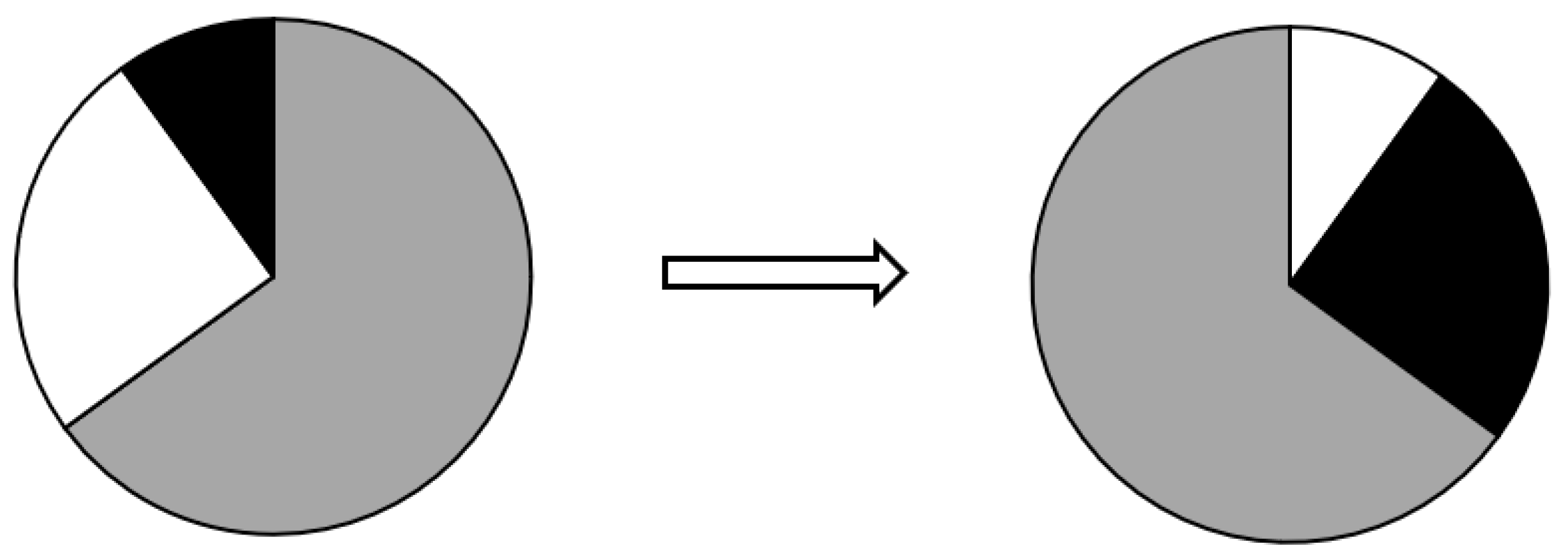
ε is related only to the geometric shape of vectors X₀ and X_k, but it is not related to their location in space;

(3)

each of the two vectors is at least minimally similar; therefore, ε is never equal to zero;

(4)

the greater the similarity between the observation vectors, the higher the value of ε;

(5)

the value of ε is equal or close to 1 when the observation vectors are parallel or when they fluctuate [28].

2.2. The Selection of Features and Respondents

Knowledge of the importance of features which affect the selection of the location of the place of residence in a city provides the basis for making the right planning and administrative decisions and for determining the directions of the development of areas and investments in the city’s development. For this reason, a study was undertaken with the aim of determining the preferences, i.e., identifying features of significance to potential buyers of a flat when selecting its location in a particular district of a city. Grey system theory focuses on incomplete information for describing the analysed research problem [12,17,30,31]. In the grey system (grey box), two categories may occur: Due to information incompleteness, or due to the uncertainty of impacts [28].

Depending on the respondent selection method, social research can have the following designs:

–

representative—when the evaluated sample is representative of the entire population,

–

quasi-representative—when the evaluated sample only partly fulfils the requirements of the representative method,

–

random—when the surveyed sample is selected in a completely random manner [32,33].

Targeted sampling is a non-random method where the respondents are selected based on specific features, such as age, sex or specific preferences. Target sampling is the preferred method when the research focuses on the behaviour, opinions and attitudes of respondents with a specific profile.

For research purposes, a random population was used, although the selection of the sample was confined to a survey of 80 people aged from 21 to 29 since it was decided that people at this age most frequently search for a place of residence. The respondents are residents of various Polish cities. The study was based on the significance of a feature in terms of the selection of the place of residence. During the study, the ranking method [34] was applied, on a scale ranging from 1 to 5, where a rating of 1 indicated the smallest impact and 5 indicated the greatest impact on the selection of the location of a place of residence.

The attributes of the survey were selected based on a study by Colquhoun of the place of residence in the United Kingdom using the following features: Threat of crime, access to health services, decent housing conditions, good shops and good public transportation [35]. Features of real estate such as a high standard of a flat, access to public transportation and access to social and service infrastructure are also assets indicated by real estate agents who present flats to be purchased or rented.

3. Results

3.1. Analysis in Terms of Input Data

For the research into social preferences, the following variables were selected:

–

threat of crime (X₁).

–

access to social infrastructure (X₂),

–

a high standard of flats (X₃),

–

convenient shopping (X₄),

–

access to public transportation (X₅),

In the first stage of the study, the presented analysis took into account the data obtained from surveys (

Table 1. Relation strength order ε for 80 observations.

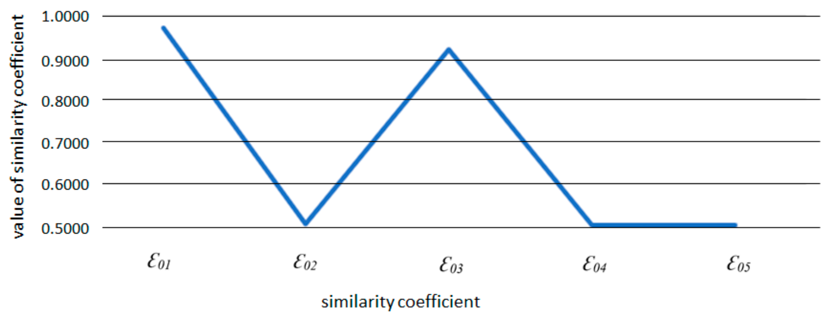
The Features that Affect the Selection of the Location of the Place of Residence in a City	The Value of the Coefficient of the System Factors’ Impact on X0
X1—criminal threats	ε01 = 0.9721
X2—access to social infrastructure	ε02 = 0.5027
X3—a high standard of flats	ε03 = 0.9201
X4—convenient shopping	ε04 = 0.5018
X5—access to public transportation	ε05 = 0.5014

Notes: Source: Own study.

).

The order of the X₁, X₂, X₃, X₄, X₅ z X₀ relation strength is as follows: ε₀₁ > ε₀₃ > ε₀₂ > ε₀₄ > ε₀₅ (Figure 2).

The obtained model reveals that the feature “threat of crime” has the greatest importance to respondents, while the feature “access to public transportation” is the least important. The selection of the location of a flat, for which the epsilon amounts to 0.9201, has a considerable effect on the selection of the location of a flat in addition to the feature of “threat of crime”, for which the epsilon value is 0.9721. The other features: X₂—access to social infrastructure, X₄—convenient shopping and X₅—access to public transportation obtained an epsilon value at a similar level, 0.5207; 0.5018 and 0.5014, respectively. The application of the grey system theory enables the determination of the significance of the impact of attributes on the selection of the location of real estate for residential purposes (as well as for making other spatial decisions, e.g., the premise that access to social infrastructure, urban transportation and service facilities are equally significant to the users of urban space).

3.2. Determination of the Relation Order for the Minimum Number of the Required Input Data

The minimum number of observations which enable the construction of a system model is four [28]. Hence, at the next stage of the study, the values of similarity coefficient ε were determined for the minimum number of observations required by the method. The selection of these observations was random; sampling from 80 observations was performed ten times. The calculated values of similarity coefficients ε are presented in

Table 2. Values of the similarity coefficient ε for four observations randomly selected 10 times.

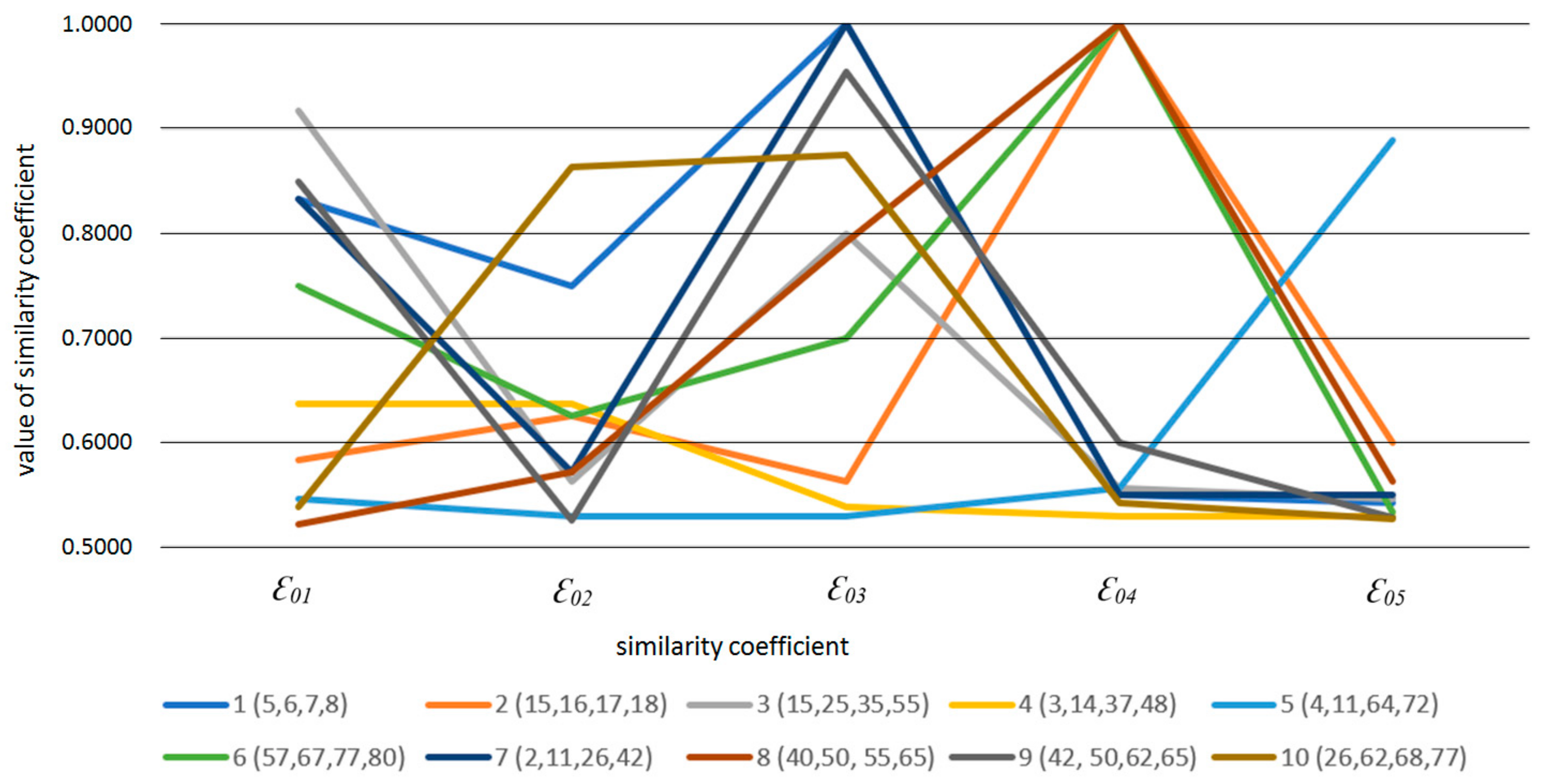
Number of Observations	ε01	ε02	ε03	ε04	ε05
1 (5,6,7,8)	0.8333	0.7500	1.0000	0.5500	0.5417
2 (15,16,17,18)	0.5833	0.6250	0.5625	1.0000	0.6000
3 (15,25,35,55)	0.9167	0.5625	0.8000	0.5556	0.5455
4 (3,14,37,48)	0.6364	0.6364	0.5385	0.5294	0.5294
5 (4,11,64,72)	0.5455	0.5294	0.5294	0.5556	0.8889
6 (57,67,77,80)	0.7500	0.6250	0.7000	1.0000	0.5333
7 (2,11,26,42)	0.8333	0.5714	1.0000	0.5500	0.5500
8 (40,50,55,65)	0.5217	0.5714	0.7917	1.0000	0.5625
9 (42,50,62,65)	0.8500	0.5250	0.9545	0.6000	0.5278
10 (26,62,68,77)	0.5385	0.8636	0.8750	0.5417	0.5263
9 (42,50,62,65)	0.8500	0.5250	0.9545	0.6000	0.5278

Notes: Source: Own study.

.

The obtained values of similarity coefficients were then recorded in the order of the relation strength (

Table 3. The order of the similarity coefficient ε relation strength for four observations randomly selected 10 times.

Sampled 4 Observations	Relation Strength Order
1 (5,6,7,8)	ε03 > ε01 > ε02 > ε04 > ε05
2 (15,16,17,18)	ε04 > ε02 > ε03 > ε05 > ε01
3 (15,25,35,55)	ε01 > ε03 > ε02 > ε04 > ε05
4 (3,14,37,48)	ε01 = ε02 > ε03 > ε04 = ε05
5 (4,11,64,72)	ε05 > ε04 > ε01 > ε02 = ε03
6 (57,67,77,80)	ε04 > ε01 > ε03 > ε02 > ε05
7 (2,11,26,42)	ε03 > ε01 > ε02 > ε04 = ε05
8 (40,50,55,65)	ε04 > ε03 > ε02 > ε05 > ε01
9 (42,50,62,65)	ε03 > ε01 > ε04 > ε05 > ε02
10 (26,62,68,77)	ε03 > ε02 > ε04 > ε01 > ε05

Notes: Source: Own study.

).

The results indicated that four observations are insufficient since the values of similarity coefficients are not ordered in an unambiguous way, which means that for particular randomly selected observations, the relation strength order for observations is different each time (Table 3). In a few cases, the epsilon values take the same values of a specific epsilon, while the other values in the sequence for a particular case already take a different position in the sequence. A similar epsilon order is observed for the case of sampling 1—ε₀₃ > ε₀₁ > ε₀₂ > ε₀₄ > ε₀₅ and 7—ε₀₃ >ε₀₁ >ε₀₂ > ε₀₄ = ε₀₅, 6—ε₀₄ > ε₀₁ > ε₀₃ > ε₀₂ > ε₀₅ and 8—ε₀₄ > ε₀₃ > ε₀₂ > ε₀₅ > ε₀₁. This means in the first case (for those selecting the location of a flat), the most important features are in the following order: A high standard of flats, threat of crime, access to social infrastructure, convenient shopping and access to public transportation, except that for the sequence in case 7, the two latter features are equally significant. In 40% of sampling cases, the most significant feature that determines the selection of a flat was a high standard of flats, with ε₀₁ taking first place in the relation strength sequence (case 1, 7, 9, 10). In 60% of cases, the feature “access to public transportation” proved to be the least significant, as ε₀₅ was last place in the sequence of significance (cases 1, 3, 4, 6, 7 and 10).

A similar trend in the similarity coefficient values can be observed in two cases for 7 (2, 11, 26, 42) and 9 (42, 50, 62, 65) (Figure 3) but, in this case, the orders of the similarity coefficient ε relation strength are not the same (Table 3).

3.3. Analysis Due to the Different Number of Observations

Another aim of the study was to examine the levels of the similarity coefficient ε values in terms of the number of observations taken into account while constructing the model. The models were constructed for 4, 5, 10, 20, 30, 40, 50, 60, 70 and 80 observations, with the values of the absolute degree of similarity ε being determined each time (

Table 4. Values of the similarity coefficient ε in terms of the number of observations.

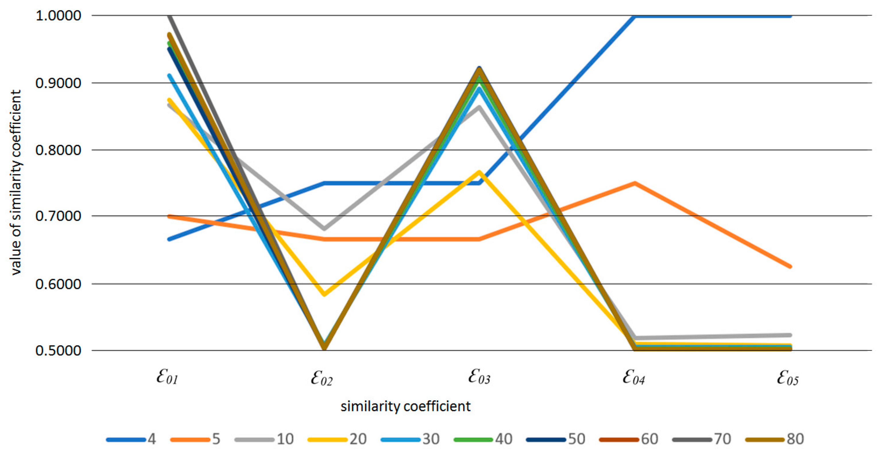
Number of Observations	ε01	ε02	ε03	ε04	ε05
4	0.6667	0.7500	0.7500	1.0000	1.0000
5	0.7000	0.6667	0.6667	0.7500	0.6250
10	0.8667	0.6818	0.8636	0.5185	0.5227
20	0.8750	0.5833	0.7667	0.5100	0.5072
30	0.9104	0.5070	0.8909	0.5051	0.5047
40	0.9593	0.5048	0.9070	0.5035	0.5030
50	0.9504	0.5035	0.9215	0.5025	0.5021
60	0.9708	0.5034	0.9197	0.5022	0.5018
70	1.0000	0.5032	0.9172	0.5020	0.5015
80	0.9721	0.5027	0.9201	0.5018	0.5014

Notes: Source: Own study.

).

It should be noted that the relation strength order is the same for observations, starting from 20 and ending with 80 (Table 4). Additional information obtained from data analysis shows that the features most significant to potential buyers of a flat include X₁, i.e., “threat of crime”, for which ε has values ranging from 0.887 to 1, and X₃, i.e., “a high standard of a flat” has ε values ranging from 0.7667 to 0.9215.

Table 5. The order of relations of the similarity coefficient ε in terms of the number of observations taken into account in the model.

Number of Observations	Relation Strength Order
4	ε04 = ε05 > ε02 = ε03 > ε01
5	ε04 > ε01 > ε02 = ε03 > ε05
10	ε01 > ε03 > ε02 > ε05 > ε04
20, 30, 40, 50, 60, 70, 80	ε01 > ε03 > ε02 > ε04 > ε05

Notes: Source: Own study.

shows the order of relations of the similarity coefficient ε in terms of the number of observations taken into account in the model.

The significance of the other features is at a balanced level, with the ε values ranging from 0.5027 to 0.5833 for feature X₂—access to social infrastructure, from 0.5018 to 0.5100 for feature X₄—convenient shopping, and from 0.5072 to 0.55014 for feature X₅—access to public transportation (Figure 4).

4. Summary

The aim of the analysis is to construct a reliable grey system model to predict its behaviour and make decisions concerning the present or the future based on the obtained order of the similarity coefficient ε relation strength. The analyses conducted determined the strength of the relations between the features adopted for the study and indicate the model’s behaviour for various numbers of input data.

Grey system theory provides tools for modelling incomplete, uncertain and scant data. The proposed method is highly effective in analysing phenomena that are characterised by incomplete data. Such data are usually encountered in spatial management processes because real-world systems are described by imperfect data. Grey systems require fewer assumptions than statistical methods, which have to fulfil numerous requirements to produce reliable results. Therefore, the proposed method poses a valuable alternative to statistical methods in spatial data analyses.

The application of the grey system methodology allows minimum data sets to be determined (data minimisation). The conducted research revealed that the minimum number of data n ≥ 4 which indicates that the application of GST was not applicable. For the data adopted for the study using a GRA-type system, a stable sequence of the order of the similarity ε relation strength was obtained for 20 observations taken into account in the model. This indicates that for the data under analysis, carrying out a survey for 20 respondents would be sufficient.

The significance of attributes determined on the basis of the similarity coefficient ε values enables the formulation of decision-making rules that can be used to develop expert systems. It also enables the development of systems for making strategic decisions and the detection of rules and observations in data sets. It also permits a more detailed pre-selection of data that cannot be used in the construction of various types of models.

The analysis of the preferences of potential buyers of real estate for residential purposes revealed that the features of the threat of crime and a high standard of a flat were the most important. The least important feature for potential buyers when selecting the location of the place of residence is the access to public transportation. The obtained information can support the decision-making process in determining the attractiveness of residential locations in a city space.

References

- Swamy, P. Statistical Inference in Random Coefficient Models; Springer: Berlin, Germany, 1971. [Google Scholar]
- Caseti, E. Generating models by the expansion method: Applications to geographic research. Geogr. Anal. 1972, 4, 81–91. [Google Scholar] [CrossRef]
- Anselin, L. Spatial Econometrics: Methods and Models; Kluwer Academic Publishers: Dordrecht, The Netherlands, 1988. [Google Scholar]
- Haining, R. Spatial Analysis of Regional Geostatistics Data; Cambridge University Press: Cambridge, UK, 2003. [Google Scholar]
- Gerus-Gościewska, M.; Gościewski, D.; Salata, T.; Palicki, S.; Prus, B.K.; Gawroński, K.; Konieczna, J.; Jaroszewicz, J.; Wilkosz-Mamcarczyk, M.; Król, K. Interpretacja Danych Przestrzennych Jako Forma Stymulowania Partycypacji Społecznej; Wydawnictwo Uniwersytetu Rolniczego: Kraków, Poland, 2015. [Google Scholar]
- Bajerowski, T.; Biłozor, A.; Cieślak, I.; Senetra, A.; Szczepańska, A. Ocena i Wycena Krajobrazu; Wydawnictwo Educaterra: Olsztyn, Poland, 2007. [Google Scholar]
- Bajerowski, T.; Bal, A.; Biłozor, A.; Gerus-Gościewska, M.; Sidor, I.; Szurek, M.; Turkowska, O.; Wielgosz, A. Teoretyczne Podstawy Teorii Gospodarki Przestrzennej i Zarządzania Przestrzenią; Bajerowski, T., Ed.; Wydawnictwo UWM: Olsztyn, Poland, 2003. [Google Scholar]
- Górniak-Zimroz, J. Wykorzystanie systemów wspomagania decyzji w gospodarce odpadami. Pr. Nauk. Inst. Gór. Politech. Wroc. Stud. Mater. 2007, 188, 23–41. [Google Scholar]
- Liu, S.; Lin, Y. Grey Information. Theory and Practical Applications; Springer: London, UK, 2006. [Google Scholar]
- Kotkowski, B.; Ratajczak, W. Zbiory Przybliżone w Analizie Danych Geograficznych. Możliwości i Ograniczenia Zastosowań Metod Badawczych w Geografii Społeczno-Ekonomicznej i Gospodarce Przestrzennej; Rogacki, H., Ed.; Bogucki Wydawnictwo Naukowe: Poznań, Poland, 2002. [Google Scholar]
- D’Amato, M. Rough Set Theory as Property Valuation Methodology: The Whole Story. Mass Appraisal Methods. An International Perspective for Property Valuers; RICS Research; Kauko, T., d’Amato, M., Eds.; Blackwell Publishing: Oxford, UK, 2008. [Google Scholar]
- Deng, J.L. Control Problems of Grey Systems. Syst. Control Lett. 1982, 1, 288–294. [Google Scholar]
- Liu, S.F.; Lin, Y. Grey Systems—Theory and Applications; Springer: Berlin, Germany, 2010. [Google Scholar]
- Liu, S.-F.; Forrest, J.; Yang, Y. A brief introduction to grey systems theory, Grey Systems: Theory and Applications. In Proceedings of the 2011 IEEE International Conference on Grey Systems and Intelligent Services, Nanjing, China, 15–18 September 2011. [Google Scholar]
- Dytczak, M.; Ginda, G. Użyteczność systemów “szarych” w transporcie i logistyce. Logistyka 2014, 3, 1515–1523. [Google Scholar]
- Deng, J. Application of Grey System Theory in China. In Proceedings of the First International Symposium on Uncertainty Modeling and Analysis, College Park, MD, USA, 3–5 December 1990. [Google Scholar]
- Donaj, Ł. Teoria szarych systemów a prognozowanie w naukach społecznych przyczynek do dyskusji. Przegląd Strateg. 2017, 7, 43–52. [Google Scholar]
- Liu, X.Q.; Wang, Z.M. Grey Econometric Models and Applications; Yellow River Press: Jinan, China, 1996. [Google Scholar]
- Liu, S.F.; Dang, Y.G.; Li, B.J. Computational analysis on the periodic contribu-tion of technological advances in Henan Province. J. Henan Agric. Univ. 1998, 32, 203–207. [Google Scholar]
- Chen, K.X. The Epistemology of Grey Medical Analysis’. Ph.D. Thesis, Huazhong University of Science and Technology, Wuhan, China, 1999. [Google Scholar]
- Tan, X.R. Grey Medical Incidence Theory and Applications. Ph.D. Thesis, Huazhong University of Science and Technology, Wuhan, China, 1997. [Google Scholar]
- Werner, K.; Mierzwiak, R.; Pochmara, J. Teoria systemów szarych jako narzędzie wspomagania prognozowania popytu. Logistyka 2009, 2. [Google Scholar]
- Wang, Z.X.; Pei, L.L. System thinking—Based grey model for sustainability evaluation of urban tourism. Kybernetes 2014, 43, 462–479. [Google Scholar] [CrossRef]
- Yang, Y.; Wang, S.W.; Hao, N.L.; Shen, X.B.; Qi, X.H. Online noise source identification based on power spectrum estimation and grey relational analysis. Appl. Acoust. 2009, 7, 493–497. [Google Scholar] [CrossRef]
- Parysek, J. Miasto w ujęciu systemowym. Ruch Praw. Ekon. Socjol. 2015, 77, 27–53. [Google Scholar] [CrossRef] [Green Version]
- Funck, R.H.; Blum, U.H. Urban Change: A Changing Process. In Klassen, Spatial Cycle; van den Berg, L., Burns, L.S., Eds.; Gower: Aldershot, UK, 1987. [Google Scholar]
- Mierzwiak, R.; Werner, K.; Pochmara, A. Zastosowanie teorii systemów szarych do prognozowania ekonomicznych szeregów czasowych. In Proceedings of the IV Krakowska Konferencja Młodych Uczonych, Sesja Plenarna Nauki Ekonomiczne, Kraków, Poland, 17–19 September 2009. [Google Scholar]
- Cempel, C. Teoria szarych systemów—Nowa metodologia analizy i oceny złożonych systemów. Przegląd możliwości. Zeszyty Naukowe Politechniki Poznańskiej 2014, 63, 9–20. [Google Scholar]
- Barczak, S. Zastosowanie teorii szarych systemów do przewidywania przyszłych ofert składanych na aukcjach pierwszej ceny poprzez pryzmat modelu szarego GM(1,1). In Studia Ekonomiczne. Innowacje w Finansach i Ubezpieczeniach—Metody Matematyczne i Informatyczne; Mika, J., Dziwok, E., Eds.; Zeszyty Naukowe Wydziałowe Wydawnictwo Uniwersytetu Ekonomicznego w Katowicach: Katowice, Poland, 2013; Volume 146, pp. 7–18. [Google Scholar]
- Barczak, S. Gold price forecasting using grey model GM(1,1) and selected classical time series models. A comparison of methods. In Proceedings of the 8th International Days of Statistics and Economics, Prague, Czechia, 11–13 September 2014. [Google Scholar]
- Deng, J. Introduction to grey system theory. J. Grey Syst. 1989, 1, 1–24. [Google Scholar]
- Mazurek-Łopacińska, K. Badania Marketingowe. Teoria i Praktyka; PWN: Warszawa, Poland, 2005. [Google Scholar]
- Wasilewska, E. Descriptive Statistics not only for Sociologists; Wydawnictwo SGGW: Warszawa, Poland, 2008. [Google Scholar]
- Bielecka, A. Statystyka w Biznesie i Ekonomii. Teoria i Praktyka; Wydawnictwo WSPiZ im. L. Koźmińskiego: Warszawa, Poland, 2005. [Google Scholar]
- Colquhoun, I. Design Out Crime: Creating Safe and Sustainable Communities. Crime Prev. Community Saf. 2004, 6, 57–70. [Google Scholar] [CrossRef]