Spatiotemporal Data Clustering: A Survey of Methods

Department of Land Survey and Geo-Informatics, The Hong Kong Polytechnic University, Kowloon, Hong Kong 999077, China
*
Author to whom correspondence should be addressed.
ISPRS Int. J. Geo-Inf. 2019, 8(3), 112; https://doi.org/10.3390/ijgi8030112
Submission received: 28 November 2018
/
Revised: 13 February 2019
/
Accepted: 24 February 2019
/
Published: 28 February 2019
Abstract
:Large quantities of spatiotemporal (ST) data can be easily collected from various domains such as transportation, social media analysis, crime analysis, and human mobility analysis. The development of ST data analysis methods can uncover potentially interesting and useful information. Due to the complexity of ST data and the diversity of objectives, a number of ST analysis methods exist, including but not limited to clustering, prediction, and change detection. As one of the most important methods, clustering has been widely used in many applications. It is a process of grouping data with similar spatial attributes, temporal attributes, or both, from which many significant events and regular phenomena can be discovered. In this paper, some representative ST clustering methods are reviewed, most of which are extended from spatial clustering. These methods are broadly divided into hypothesis testing-based methods and partitional clustering methods that have been applied differently in previous research. Research trends and the challenges of ST clustering are also discussed.
1. Introduction
Large-scale data mining brings new opportunities and challenges for discovering hidden valuable information from enormous data sets. In particular, with the rapid development of positioning technologies as well as the emergence of a large number of positioning devices, a vast amount of data could be easily collected from different sources. These sources could come from broad domains, including government documentary and decades of collected data, transportation [1], and social media [2]. For example, governments conduct censuses and own large datasets containing information about population change, human movement, and economic characteristics during different periods for planning and policy making. Many floating cars such as taxi and truck installing GPS receivers can monitor running state and record spatial and temporal information every second. Social media like Facebook and Twitter can post users’ experiences at a given place and time. All this spatiotemporal information is useful for pattern analysis in space and time. Space can be represented by an address, geographical coordinates of latitudes and longitude, or local () coordinates. Time can be shown by year, month, and day and sometimes as detailed as hour, minute, or second. Spatiotemporal (ST) data types can be divided into five categories containing events, geo-referenced variables, geo-referenced time series, moving points, and trajectories [3] (Figure 1). The collected datasets, regardless of if they are in tabular or graphical forms, are often too complex to be understood. An efficient spatiotemporal analysis method is important to mine meaningful patterns for better understanding or visualization [4].
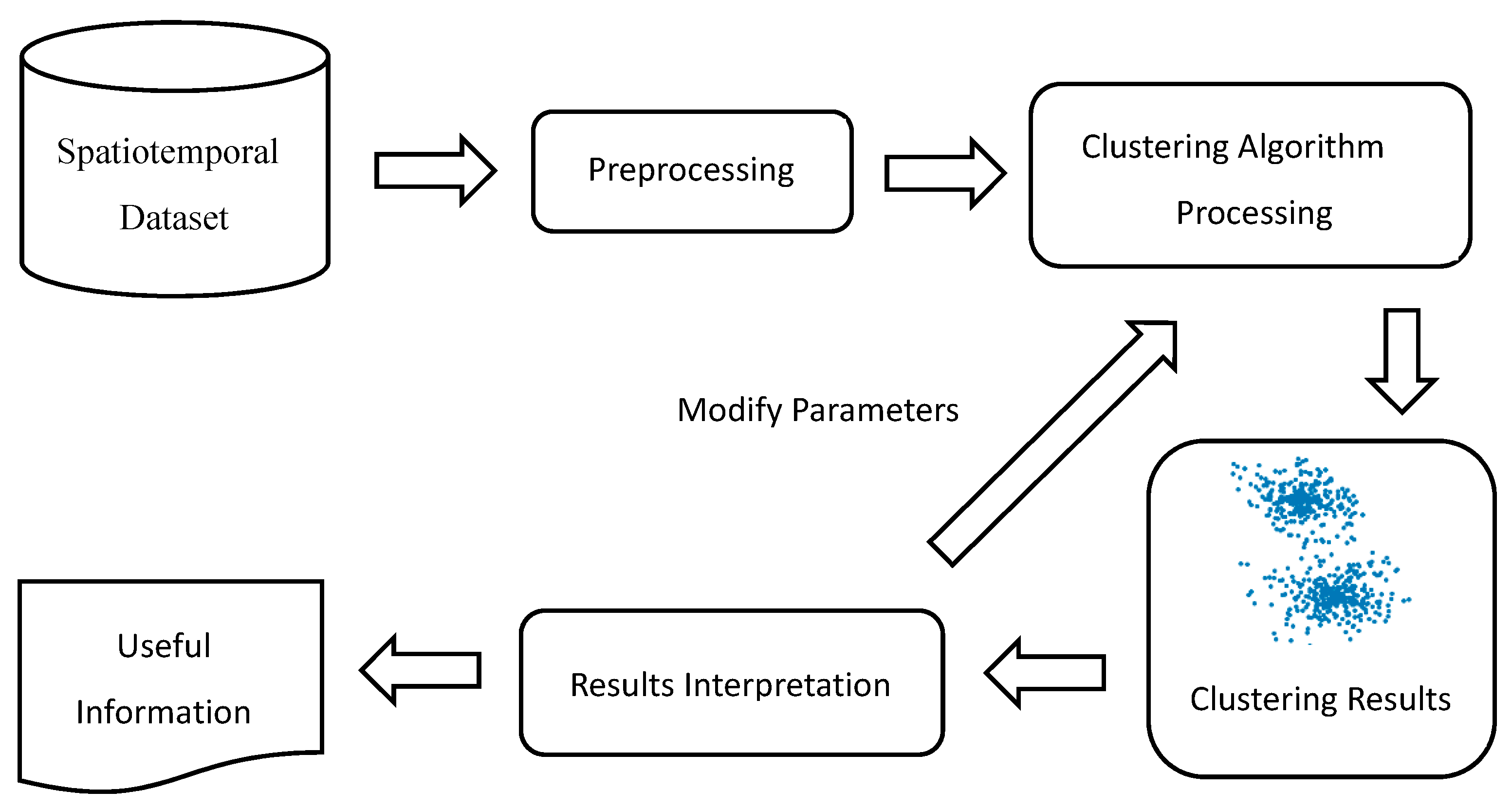
A good approach is to put data with similar characteristics together to find interesting and useful features. Clustering is one popular unsupervised method for discovering potential patterns and is widely used in data analysis, especially for geographical data [5]. It aims to group events according to neighboring occurrence and/or similar attributes. Most clustering algorithms should measure the distance between each pair. Various distance functions are adopted in the clustering methods, such as the Euclidean and Manhattan distance functions. A famous application of clustering occurred in 1854, when Dr John Snow found that clusters of cholera cases occurred around a public water pump, which was the source of the spread of cholera. Clustering is a high-performance tool for detecting hot spot patterns in spatial/ST data analysis [6]. ST data analysis methods can be classified into six categories—clustering, prediction, change detection, frequent pattern mining, anomaly detection, and relationship mining [7]. Clustering has been used in many applications [8]. In some cases, spatiotemporal clustering methods are not all that different from two-dimensional spatial clustering [9,10,11]. Figure 2 shows the procedure of clustering. For raw spatiotemporal data, the first step is cleaning and reorganization. Incorrect and missing data should be identified and deleted before applying an appropriate clustering algorithm. However, different parameters can affect the clustering results. It is necessary to adjust parameters for a better understanding of cluster results and interpreting potential information.
There are still many challenges for extracting useful ST patterns due to complex data types. Many methods simply treat the temporal dimension of spatiotemporal data as an additional dimension. With different units of time and space, clustering results could have big differences when considering the scale of time. Multiple scales effect is another challenge as the clustering results depend on the various spatial and temporal scales. Different space regions and temporal periods could form distinguished clusters.
In this paper, we only focus on the clustering methods of the events ST data type. In our view, these could be divided into two categories, the hypothesis testing-based methods and the partition-based methods. The former one mainly uses a probability model and statistical hypothesis testing to find significant clusters. In general, the null hypothesis is that the distribution of events is random; if it is rejected, a cluster could be formed. The partitional clustering methods mostly utilize distance functions to compute the closeness of events to distinguish cluster and noise. Some popular spatiotemporal clustering methods are introduced in the following sections. This will help to understand the evolution of techniques in the past decades and explore future research trends.
2. From Spatial to ST Clustering
In this section, we will first briefly discuss spatial clustering. There is no clear definition of clustering [12,13] and different categories have overlap such that an algorithm could contain more than one feature of categories. Therefore, a lot of methods have been proposed according to diverse principles. Han, et al. [6] divided major clustering methods into four categories, which were partitioning methods, hierarchical methods, grid-based methods, and density-based methods. Partitioning methods divide the entire dataset into several groups. For example, K-means is the most popular clustering method in the partitioning methods. It is an iteration process to find the cluster and its center. Based on this theory, Kaufman and Rousseeuw [14] proposed partitioning around medoids (PAM) and clustering large application (CLARA) to improve the efficiency of clustering. Ng and Han [15] proposed clustering large applications based upon randomized search (CLARANS) to investigate not only detect points but also polygon objects. Hierarchical methods can separate a dataset into multiple levels based on distance or density functions. For example, Balanced iterative reducing and clustering using hierarchies (BIRCH) use a tree structure to form clusters with speed and efficiency [11]. Chameleon finds the clusters by measuring the similarity of data and grouping them [16]. Clustering using Representatives (CURE) [17] can identify non-spherical shapes of clusters within a large database. Density-based methods have the ability to discover different shapes of clusters. For example, density based spatial clustering of applications with noise(DBSCAN) [18] is a well-known algorithm for detecting an arbitrary shape of clusters, and many people have proposed improved methods to overcome any drawbacks and promote efficiency [19,20,21,22]. DBSCAN is sensitive to input parameters, however, ordering points to identify the clustering structure (OPTICS) [9] could prevent this problem from affecting the clustering results. However, it cannot get accurate cluster results. A method called DENCLUE (Density-based clustering) uses a kernel density estimation model to identify the high density of clusters with an arbitrary shape. Grid-based methods build a grid structure for storing the dataset and each grid is the basic unit to form a cluster [23,24]. Asides from the four categories, many other methods have also been proposed, such as model based methods [25,26].
The major difference between spatial and ST clustering is the ‘time’ element, which is treated as either another dimension or an attribute. By space, it can be at least 2-dimensional (,) or 3-dimensional (,,) in which events or attributes are clustered. Most socio-economic information, such as population and traffic, is considered as variations in 2-dimensions [(,) + attribute] only; whereas natural phenomena, such as temperature and pressure, vary with space and height [(,,) + attribute]. When ‘time’ is added, it may be treated as merely an attribute to 2-dimensional or 3-dimensional space, for example, a date when a certain event occurs or a record is created; but this does not allow clustering in terms of time. An alternative common method is to model ‘time’ as a third dimension in addition to the 2-dimensional [(,) + attribute] space. Therefore, some ST clustering methods have been developed from spatial clustering methods [27,28,29,30]. The addition of a time dimension to the 3-dimensional [(,) + attribute] space is still a challenging issue to model and to visualize. There is a need in many applications to integrate spatial and temporal information together for more detailed and accurate analyses. For example, in the study of human mobility, there is a need to identify at what time and where people cluster instead of just relying on census data or a generalized pattern of population distribution. This applies in the same way to crime patterns, traffic patterns etc. In the following sections, we will discuss the different categories of ST clustering.
3. Hypothesis testing-based methods
In the field of statistics, some existing fundamental research has been studied [31], including ST point pattern detection and analysis [32,33]. Hypothesis testing is used to determine the probability of a given hypothesis being true or not. The advantage of this method is it considers space and time information together. It is a new research direction that could allow some traditional spatial statistics to be extended for ST data analysis. For example, Di Martino and Sessa [34] proposed an extended algorithm of fuzzy c-means to find circular clusters from ST data. This method could reduce the noise and outliers influencing clustering results. Detailed processes of some famous algorithms are described below.
3.1. Space–time interaction methods
A number of methods have been explored for detecting ST clustering. The core essence of a cluster is that objects should be close to each other in the space or time dimension. Knox and Bartlett [35] proposed a test to quantify a space and time interaction of disease. Low-intensity disease detection by joining space and time analysis was conducted in Reference [36]. Improvements to existing drawbacks were proposed by others [37]. In this method, critical space distance α and time distance β should be manually defined first. Pairs of cases less than the critical space distance and time distance separately were regarded as near in space and time. The test statistics equation was:
where K was the total number of paired cases smaller than the critical space and time distance, N was the total number of data. dij was space adjacency, if the distance between i and j was less than α, it was equal to 1, otherwise equal to 0. tij was time adjacency, if the distance between i and j was less than β, it was equal to 1, otherwise equal to 0. The Monte Carlo method was used for the significant test of and a predefined number of runs was identified. The probability value of K being larger than the test statistic should belong to right hand tail of null distribution. The disadvantage of this method was critical space and time distances values may be assigned subjectively.
A modification was proposed by Mantel [38] who multiplied the sum of time distances by the sum of spatial distances. The test statistic of Mantel’s test was similar to Knox’s test. It focused on the problem of selecting the critical distances of Knox’s test. It is based on a simple cross-product term:
where is the distance between data and in space. is the distance between data and in time. Then, it is normalized:
where is the standardized Mantel statistic and N is the number of data. is the distance between data i and j in space. is the distance between data i and j in time. is the average distance of all data in space. is the average distance of all data in time. and are the standard deviations of data in space and time, respectively. This equation allowed for different units of space and time in the same framework, and multiple scale problems could be solved by limiting the range of correlation coefficient values into [−1,1].
3.2. Spatiotemporal k Nearest Neighbors Test
Jacquez [39] proposed a spatiotemporal k nearest neighbors test to test space and time simultaneously. The statistic counted the number of k nearest neighbors in space and time dimension and evaluated under the null hypothesis of independent in two dimensions. Two test statistics were defined, which are and . is the count of case pairs of k nearest neighbors. It is large when space and time interact. is the count number of difference between consecutive k nearest neighbors. Some concepts are as follows:
- N: Number of cases.
- dij: Spatial measure, when case is a nearest neighbor of case in space, otherwise equal to 0.
- tij: Spatial measure, when case is a nearest neighbor of case in time, otherwise equal to 0.
- : Is a cumulative test statistic, where .
- : Is specific test statistic, where .
was not independent because it included a smaller value of nearest neighbor. was independent because it only contained specific nearest neighbors. The null hypothesis was that the distribution of events was independent from each other in space and time. Reference distribution was built by repeating many times to generate a random distribution for testing the statistics of probability values by comparing and . However, the disadvantage of this method was that the value could result in different test results.
3.3. Scan Statistics
Scan statistics is a popular method and software [40] can implement scan statistics for detecting clusters. Joseph Naus [41] has been called the father of scan statistics as his method has helped to solve many research problems. The space scan statistic was developed from an original scan statistics method based on the scanning window process [42]. A circular scan window with different radii is used to find circular clusters of two-dimensional spatial data with a statistical significance test. An appropriate radius is important to avoid too large or too small clusters, otherwise the results could be meaningless and hard to interpret. Normally, the upper limit of the circle should not include more than 50 percent of all the dataset. Each point could be the center of a circle that contains different numbers of other points. Space and space–time scan statistics have many similar calculation processes.
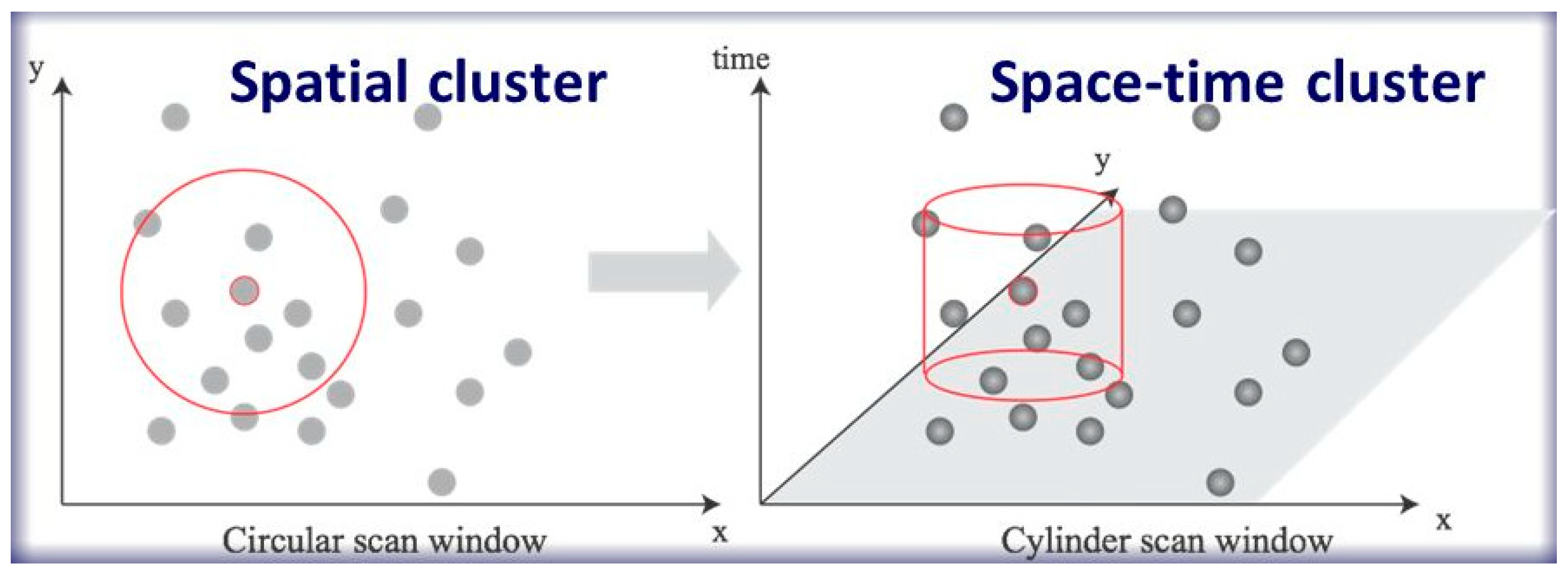
Space–time scan statistics was extended from space scan statistics to detect clusters with the highest likelihood ratio by moving a cylinder as a scan window to scan ST data [43,44]. Figure 3 shows the difference between the two methods. The left graph uses space scan statistics to detect clusters, the red center is the core point and the larger circle is the scan window for detection. The right graph uses space–time scan statistics to find clusters, it adopts a red cylinder as the scan window. Space–time scan statistics considers the time dimension and is an extension of space scan statistics in that a three-dimensional cylinder instead of a two-dimensional circle is used. The time interval between events is the height of cylinder.
As with the space scan statistic, the null hypothesis is that the spatiotemporal distribution of events is random. The scan window of the cylinder was changed with different radii and height, looking for the maximum value of log likelihood ratio of all the circles as the cluster region. The formulation was:
where S was the log likelihood of cylinder, and were the observed and expected number of points, respectively, N was the total number of observed points, and I was the indicator function. If the left side was larger than right side, I was equal to , otherwise equal to 0. Many distribution functions could be used, one of which was the Poisson distribution. To obtain the simulated distribution for significance testing of clusters, Monte Carlo replications of data were used to obtain likelihood ratio statistics S. It was necessary to obtain values by generating replications such as 999 or even higher to calculate the probability of a random appearance of an observed high-density cluster in a cylindrical window. The likely clusters could be based on the lowest value, which was defined by the cylindrical window. However, similar to space scan, the disadvantage of this method was that it could not discover the arbitrary shape of ST data. To overcome this problem, flexible spatial scan statistic [45] and flexibly shaped space–time scan statistic [46] were proposed in 2005 and 2008, respectively. FleXScan [47] is the software that was developed to analyze spatial data by using flexible spatial scan statistics. Compare with spatial and space–time scan statistics that can only detect circular or cylinder clusters with variable size, these two methods have the ability to detect non-circular and non-cylinder clusters with high accuracy. For example, Tango and Takahashi [45] proposed a flexible spatial scan statistics method that was illustrated using simulated disease maps in the Tokyo Metropolitan area. First, they divided the entire area into many small regions and the location of each region was the administrative population centroid. Next, the set of irregularly shaped windows were consisted concentric circles and connected regions, where is a pre-specified maximum length of cluster. The idea was also used in the flexible space–time scan statistic. However, both of these were fitted to a small cluster size. Neill [48] gave a very comprehensive account of spatial and ST clustering methods, especially in the area of scan statistics methods and Bayesian clustering methods. They proposed a statistical framework for detecting clusters in detail. The results of case studies show it has good performance compared to previous studies. However, they are still subject to the limitations of statistical methods.
4. Partitional Clustering Methods
In the previous section, clustering of hypothesis testing-based methods was developed based on mathematical theory of probability and statistics. In this section, partitional clustering methods are introduced. These methods mainly focus on identifying whether data belong to a cluster or noise by using different distance functions. They have a clear grouping process to form a cluster by determining the similarity of data. Some well-known methods are described as follows:
4.1. DBSCAN
DBSCAN is a very popular method, especially in the data mining community [5,6]. It has been extended for many different types of data. The biggest advantages of this method is that it can find clusters with arbitrary shape and noise points [18]. The key idea is that each cluster should include at least a minimum number of points with a fixed radius. Similar to kernel density estimation (KDE), DBSCAN can also be extended for spatiotemporal data. ST-DBSCAN [27,49] was proposed to cluster spatiotemporal data. Wang, et al. [49] added another radius which is the temporal neighborhood radius. The core points should satisfy directly the density reachable in both spatial radius and temporal radius .
To define an appropriate spatial and temporal radius, k-dist graph was used to decide values. Generally speaking, cluster data should be clearly separated from noise data. To do this, the distance of each point to its k nearest neighbor, called the k value, was calculated. As depicted in Figure 4, the left graph shows the distribution of point sample, clearly indicating three similar density clusters surrounded by noise points. The right graph was drawn based on a descending order of k values. The smooth red line on the right part of the graph highlights cluster points that have a low k value, but the left part of the red line indicates noise points that have high values. An appropriate threshold could be selected from the graph with an obvious and abrupt change from high value of small number of points to low value of large number of points.
Another method was called ST-GRID. The core idea was that a three-dimensional grid covers the entire dataset followed by merging the dense neighboring cells. First, the above k-dist graph could be used to define the border length of the grid and put all the data into a multi-dimension grid. Second, the number of points in each cell was counted. Those equal or larger than were merged with neighbor cells as a cluster. The process was repeated until no additional cells could be merged.
Compared with the above method, more detailed data such as non-spatial data should be considered when extending DBSCAN [27,50]. A new method called ST-DBSCAN was proposed for discovering clusters based on three attributes; non-spatial, spatial, and temporal attributes of data. Basic concepts were the same as conventional DBSCAN except for three modifications.
When DBSCAN only considers one distance parameter to find similar data, ST-DBSCAN used two distance parameters for two-dimensional data. One distance measured two points distance in spatial scale. Another distance measured non-spatial attributes. Euclidean distance was adopted to calculate the two distances.
where x and y represented spatial information. DBSCAN algorithm’ result could be affected by selecting a different radius. If the dataset included different densities of clusters, a single radius could not clearly identify each cluster. To solve the problem, they proposed a concept called the density factor. Each cluster has their own density factor. To calculate it, three concepts of distances are introduced, which are density_distance_max, density_distance_min and density_distance. Density_distance_max was the maximum distance between object p and its neighbor objects within the radius Eps. Density_distance_min was the minimum distance of each cluster. The density_distance of object p was defined as density_distance_max ()/density_distance_min (). The density_factor was defined as follows.
The density_factor C denoted the degree of each cluster. If the points of a cluster were close to each other, density_diatance_min would decrease, the density_distance would be quite large, and the density_factor would be close to 0. Otherwise, if points were a little further away from each other, the density_distance would be quite small and the density_factory would be close to 1.
For non-spatial values of objects, this added value could change the average value of existing points when clustering. To solve the problem, ST-DBCSAN compared the average value of a cluster with every other point. If the absolute difference between the average value and object value was larger than a threshold, that point should not to be contained in the cluster.
4.2. Kernel Density Estimation
Kernel density estimation (KDE) [51,52] is a nonparametric density estimation method widely used for detecting clusters from spatial data to discover high-density significant geographic events. Gaussian function is an efficient and popular choice for kernel density estimation. The KDE equation can be extended as follows:
where was the number of sample data, meant the bandwidth parameter, and was the kernel density functions. Many kernel functions had been defined for different situations. An appropriate bandwidth could lead to a good density result. The function of Scott’s rule of thumb was used to calculate bandwidth with the equation as follows:
where was the standard deviation of sample data, and meant the number of sample data. This rule of thumb was very easy to compute and could be accepted as an accurate estimator. There are mainly two ways to extend KDE for spatiotemporal data by adding a time dimension (Table 1).
Conventional KDE should be extended by adjusting the parameters for spatiotemporal data. Brunsdon, et al. [53] extended the two-dimensional KDE into three-dimensional for space and time data analysis. It helped to visualize and understand the trend of spatiotemporal data. The three-dimensional spatiotemporal KDE formula was:
where the notation was the same as Equation (5), was the kernel function for time, was the bandwidth parameter of time kernel. Spatial and temporal information were treated separately, each of which had its own bandwidths and kernel functions. Nakaya and Yano [54] adopted this method for visualizing high-density crime events during a specific time interval in Kyoto. A threshold was set to filter data beyond a defined range. For most data, the longer space/time distance between two datasets, the lower possibility of their correlation. For example, if the time distance of two adjacent data was larger than a threshold, there was no need to calculate kernel density. The advantage of this method was no requirement to define a density function of time, but time was regarded as a constant. The formula was:
In this formula, only kernel density of space needs to be calculated. However, it is difficult to define an appropriate method for filtering time. In order to directly integrated space and time data, the process of standardization should be conducted before density estimation with the following equations:
and,
where , were spatial and temporal raw data, , could be referenced values for standardizing raw spatial and temporal data and , were their kernel bandwidths. The advantage of standardization of raw spatial and temporal data was to remove the different measurement units of spatial and temporal data. The results of standardization of spatial and temporal data was that they have similar ranges for easy integration. The calculation of kernel density estimation was
However, it is noted that bandwidth selection was a critical problem that will affect cluster results. The unit of time was another problem because different units lead to different density of clusters.
4.3. Windowed Nearest Neighbor Method
Based on the idea of spatiotemporal nearest neighbors test, windowed nearest neighbor method for mining spatiotemporal clusters was proposed several years ago [56]. Spatiotemporal point data could be represented by , each point indicated by , and its neighbor could be defined as:
For nearest neighbors, the time interval of consecutive two points should be smaller than a threshold, . The distances from a given point to the rests are gradually increasing with time satisfied as:
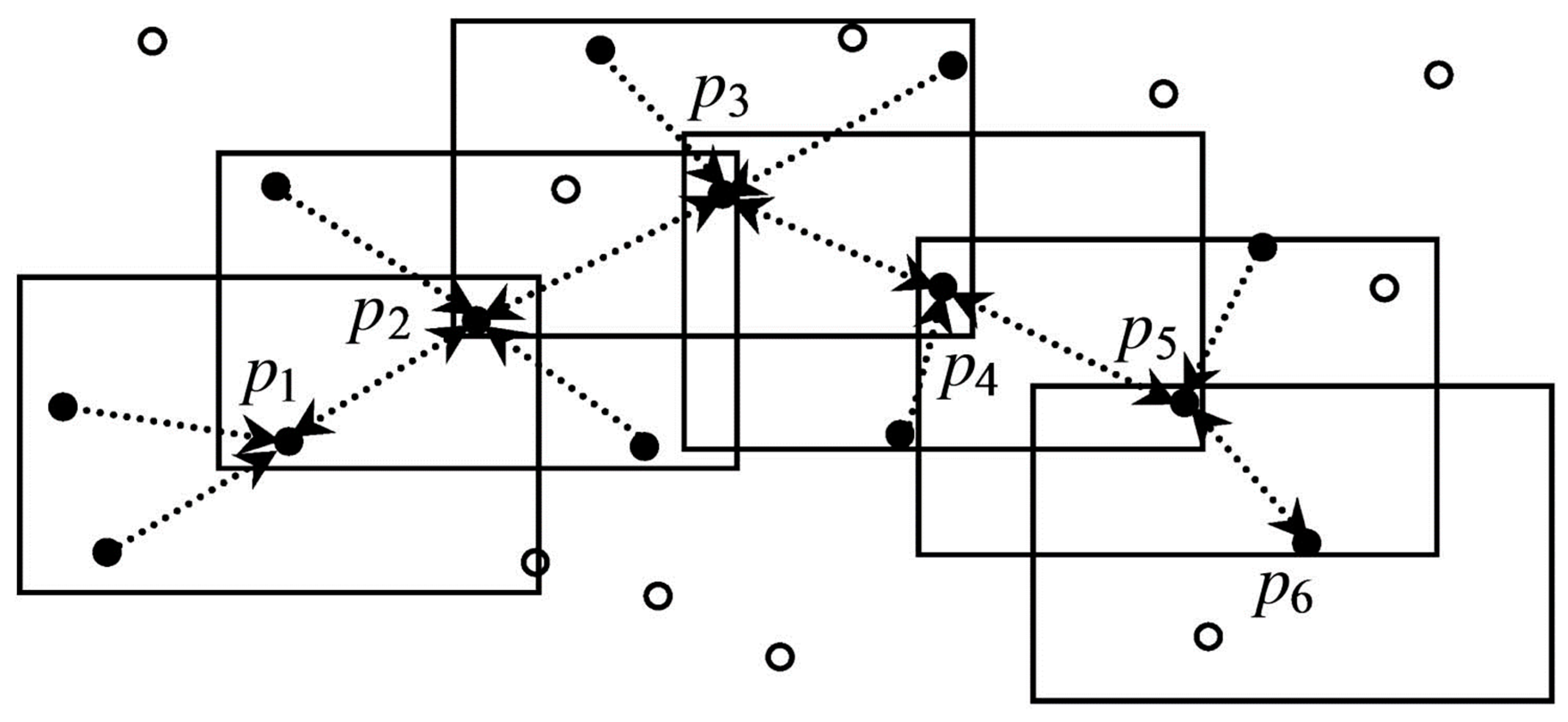
Similar to space–time scan statistics, each event could be regarded as a center of cylinder with a spatial radius and temporal height. A cylinder as a window includes spatiotemporal neighbors of a given event. A core event’s neighbor should contain a minimum number of other points. The first step is to distinguish between a cluster of events and noise; second is to connect the cylinder into cluster events. Figure 5 shows the spatiotemporal density connectivity of events from a horizontal perspective to form the cluster.
In their method, an ST Poisson point process was used to construct probability density function with the equation:
where was the number of events in the volume of , was the constant. The density of cylinder can be calculated by:
where was the number of events, and was the temporal interval constant. could be regarded as a threshold calculated by an expectation maximization (EM) algorithm [57]. A detailed process of the EM algorithm can be found in Byers and Raftery [58]. After the density connected events were divided into cluster events and noise features, they were linked by the cylinder for connecting events into clusters.
5. Applications
ST data clustering methods are widely used in many research areas, which we have divided into the following categories.
Crime analysis: Criminal events usually repeatedly occur under the same situation and a similar time. Tracing the changes of a crime path is meaningful. Nakaya and Yano [54] explored the possibility of tracing crime events with three-dimensional attributes in a space–time cube relative to kernel density estimation and scan statistics to get the clustering of crime events and visualizing the crime events patterns. Hu, et al. [28] proposed a new modification of an existing method to increase the predictive accuracy of crime hotspots. They refined spatiotemporal kernel density estimation by generalized product kernels and adopted a data driven bandwidth selection to decide bandwidth. Residential burglaries data of Baton Rouge was used to predict crime hotspots.
Events detection: Many events could be detected using clustering methods, such as helicopter crash accidents from social media data [59]. By using space–time scan statistics, a ST significant cluster of London helicopter crash locations were found. Many other events like football games and train and flight delays could also be detected. Clustering earthquake events could help to understand trends and mechanisms [60,61]. Many small earthquakes can happen before or after a strong earthquake. By using ST clustering methods, clusters of earthquakes can be identified in space and time. ST kernel density estimation can be used for predicting ambulance demand. It is difficult to predict ambulance demand accurately from large-scale datasets of past events. Zhou and Matteson [62] proposed a model of spatiotemporal kernel density predictive method to explore ambulance demand precisely. KDE is also widely used in creating a density map of road accidents to identify its distribution pattern [63]. This could help to predict and reduce the number of incidents in the future.
Mobility: Human mobility data such as phone call data could reflect urban growth in space and time. It would provide information for authorities to plan and manage cities in a smart way. It helps planners to understand where and when different groups of people interact in urban space. Jiang, et al. [64] discovered the clusters of human mobility pattern by kernel density estimation and integrating various spatial and temporal data to predict human daily routines. Krisp, et al. [65] proposed directed kernel density estimation to recognize movement and direction of crowds and was effective in visualizing the movement of crowds.
Disease analysis: ST clustering methods could be applied in analyzing disease dispersion and trends. Visualizing space–time clusters of dengue fever pattern in Cali using extension of kernel density estimation method has been applied [66,67]. The occurrence and spread of disease has a strong regular pattern in certain regions. Analyzing the former spread of disease to predict the future spread direction is meaningful for governments and hospitals to control diseases. Gomide, et al. [68] analyzed not only the location and time the disease was contracted, but also the reaction of the population when facing the disease. They used the ST-DBSCAN clustering method to explore the ST distribution characteristics of disease incidents to group nearby cities that have similar incident rates. A linear regression model was built to predict the number of diseases using the proportion of user experiences. Napier, et al. [69] proposed a novel Bayesian model to identify the cluster of similar temporal disease trends rather than disease estimation and prediction. Adin, et al. [70] proposed a two-stage approach to estimate disease risk maps. Compared with traditional methods, their method has the ability to overcome the problem of local discontinuities in the spatial pattern that cannot be modeled. It has a good performance of spatiotemporal smoothing for estimating risks of disease mapping.
6. Conclusion and Future Works
ST data clustering analysis is a hot topic and has already been studied extensively [71]. ST data types can be classified into three categories, namely point, line, and polygon. In this paper, only point pattern is considered and existing clustering methods are divided into two parts, one is hypothesis testing based, and another is partitional clustering methods. ST data is more complicated than other types of data because of the additional dimension of time from two-dimensional spatial analysis. Some popular and representative methods are introduced in previous sections. However, simply regarding time as an extended dimension may ignore some important patterns that are hard to be detected. New methods should consider integrating time and other attributes together.
Clustering is an important step to detect patterns from a large amount of data. It can be used in many application domains, including transportation, social media, and urban development. It focuses on finding hotspots from raw data. These hotspots are the foundation for pattern understanding. Adjusting different parameters of the clustering method for different data types is needed to get an optimum result. An appropriate clustering method can help discover potential and useful information from a large volume of data. Asides from investigating new algorithms, related research problems have been developed, such as the computational issues of ST data [72]. As mentioned before, even though extended algorithms could be used to detect clusters, these are more than mere geometrical considerations. There is a need to predefine thresholds such as radius, distance, and density based on the rules or knowledge from specific themes. As such, new research trends and methods need to be developed.
ST data analysis has attracted much research attention and a lot of methods have been developed [73]. However, there are still some issues and challenges to be solved. Several challenge issues are described as follows:
- Multiple scales clustering of ST data is an important research topic. Clustering results could be different with both changing map scales and data scale of nominal, ordinal, interval, or ratio value (i.e., with increasing attribute information). The problem of multiple scales is related to different shapes, sizes, and densities of event distribution. A changing clustering algorithm with changing scales for different applications is worth investigating in the future.
- Modifiable areal unit problem is still a problem in clustering. It has a strong relationship with scale selection. With different units of spatial and temporal data, clustering results could be variable with the choices of appropriate spatial and temporal units. Especially for temporal information, diverse time periods could indicate different cluster patterns. The identification of optimal spatial and temporal units should be considered.
- Different types of ST data analysis should be considered to develop diverse clustering methods. In many existing studies, most algorithms are focused on point features or events. However, trajectory data from GPS and other positioning equipment can record locational information in a linear dimension, thus demanding new methods for line clustering. The same applies for outliers’ detection [74,75] and classification algorithms that have not been investigated thoroughly yet.
- Different patterns could result from using different methods or time periods. It is difficult to detect the best pattern based on one algorithm. Generally speaking, raw data could contain many different kinds of pattern. For efficient mining of potential patterns, new algorithms for evaluating the accuracy or reliability of various patterns should be investigated in the future.
- Clustering methods for multiple dimensional data beyond the third dimension need to be developed for analysis and visualization.
Author Contributions
Conceptualization, L.S.C.P.-C., Z.S.; writing—original draft preparation, Z.S.; writing—review and editing, L.S.C.P.-C., Z.S.
Funding
The work described in this paper was substantially supported by grants from the Hong Kong Polytechnic University, project numbers G-YBN7 & G-YBU5.
Acknowledgments
Our deepest gratitude goes to the anonymous reviewers and editors for their insightful suggestions.
Conflicts of Interest
The authors declare no conflict of interest.
References
- Zheng, Y. Trajectory data mining: An overview. ACM Trans. Intell. Syst. Technol. 2015, 6, 29. [Google Scholar] [CrossRef]
- Tang, J.; Chang, Y.; Liu, H. Mining social media with social theories: A survey. ACM SIGKDD Explor. Newsl. 2014, 15, 20–29. [Google Scholar] [CrossRef]
- Kisilevich, S.; Mansmann, F.; Nanni, M.; Rinzivillo, S. Data Mining and Knowledge Discovery Handbook; Springer: Berlin/Heidelberg, Germany, 2009. [Google Scholar]
- Shekhar, S.; Evans, M.R.; Kang, J.M.; Mohan, P. Identifying patterns in spatial information: A survey of methods. Wiley Interdiscip. Rev. Data Min. Knowl. Discov. 2011, 1, 193–214. [Google Scholar] [CrossRef]
- Miller, H.J.; Han, J. Geographic Data Mining and Knowledge Discovery; CRC Press: Boca Raton, FL, USA, 2009. [Google Scholar]
- Han, J.; Pei, J.; Kamber, M. Data Mining: Concepts and Techniques; Elsevier: Amsterdam, The Netherlands, 2011. [Google Scholar]
- Atluri, G.; Karpatne, A.; Kumar, V. Spatio-Temporal Data Mining: A Survey of Problems and Methods. ACM Comput. Surv. 2017, 1. [Google Scholar] [CrossRef]
- Cheng, T.; Haworth, J.; Anbaroglu, B.; Tanaksaranond, G.; Wang, J. Spatiotemporal data mining. In Handbook of Regional Science; Springer: Berlin/Heidelberg, Germany, 2014; pp. 1173–1193. [Google Scholar]
- Ankerst, M.; Breunig, M.M.; Kriegel, H.-P.; Sander, J. OPTICS: Ordering points to identify the clustering structure. In Proceedings of the ACM SIGMOD Record, Philadelphia, PA, USA, 31 May–3 June 1999; pp. 49–60. [Google Scholar]
- Pei, T.; Jasra, A.; Hand, D.J.; Zhu, A.-X.; Zhou, C. DECODE: A new method for discovering clusters of different densities in spatial data. Data Min. Knowl. Discov. 2009, 18, 337–369. [Google Scholar] [CrossRef]
- Zhang, T.; Ramakrishnan, R.; Livny, M. BIRCH: An efficient data clustering method for very large databases. In Proceedings of the ACM SIGMOD International Conference on Management of Data, Montreal, QC, Canada, 4–6 June 1996; pp. 103–114. [Google Scholar]
- Rokach, L.; Maimon, O. Clustering methods. In Data Mining and Knowledge Discovery Handbook; Springer: Berlin/Heidelberg, Germany, 2005; pp. 321–352. [Google Scholar]
- Saxena, A.; Prasad, M.; Gupta, A.; Bharill, N.; Patel, O.P.; Tiwari, A.; Er, M.J.; Ding, W.; Lin, C.-T. A review of clustering techniques and developments. Neurocomputing 2017, 267, 664–681. [Google Scholar] [CrossRef]
- Kaufman, L.; Rousseeuw, P.J. Finding Groups in Data: An Introduction to Cluster Analysis; John Wiley & Sons: Hoboken, NJ, USA, 2009; Volume 344. [Google Scholar]
- Ng, R.T.; Han, J. CLARANS: A method for clustering objects for spatial data mining. IEEE Trans. Knowl. Data Eng. 2002, 14, 1003–1016. [Google Scholar] [CrossRef]
- Karypis, G.; Han, E.-H.; Kumar, V. Chameleon: Hierarchical clustering using dynamic modeling. Computer 1999, 32, 68–75. [Google Scholar] [CrossRef]
- Guha, S.; Rastogi, R.; Shim, K. CURE: An efficient clustering algorithm for large databases. In Proceedings of the ACM SIGMOD International Conference on Management of Data, Seattle, WA, USA, 1–4 June 1998; pp. 73–84. [Google Scholar]
- Ester, M.; Kriegel, H.-P.; Sander, J.; Xu, X. A density-based algorithm for discovering clusters in large spatial databases with noise. In Proceedings of the Proceedings of the 2nd International Conference on Knowledge and Discovery and Data Mining, Portland, OR, USA, 2–4 August 1996; pp. 226–231.
- Gaonkar, M.N.; Sawant, K. AutoEpsDBSCAN: DBSCAN with Eps automatic for large dataset. Int. J. Adv. Comput. Theory Eng. 2013, 2, 11–16. [Google Scholar]
- Ghanbarpour, A.; Minaei, B. EXDBSCAN: An extension of DBSCAN to detect clusters in multi-density datasets. In Proceedings of the 2014 Iranian Conference on Intelligent Systems (ICIS), Bam, Iran, 4–6 February 2014; pp. 1–5. [Google Scholar]
- Liu, P.; Zhou, D.; Wu, N. VDBSCAN: Varied density based spatial clustering of applications with noise. In Proceedings of the International Conference on Service Systems and Service Management, Chengdu, China, 9–11 June 2007; pp. 1–4. [Google Scholar]
- Ruiz, C.; Spiliopoulou, M.; Menasalvas, E. C-dbscan: Density-based clustering with constraints. In Proceedings of the International Workshop on Rough Sets, Fuzzy Sets, Data Mining, and Granular-Soft Computing, Toronto, ON, Canada, 14–16 May 2007; pp. 216–223. [Google Scholar]
- Sheikholeslami, G.; Chatterjee, S.; Zhang, A. Wavecluster: A multi-resolution clustering approach for very large spatial databases. In Proceedings of the VLDB, New York, NY, USA, 24–27 August 1998; pp. 428–439. [Google Scholar]
- Wang, W.; Yang, J.; Muntz, R. STING: A statistical information grid approach to spatial data mining. In Proceedings of the International Conference on Very Large Data Bases (VLDB), New York, NY, USA, 24–27 August 1998; pp. 186–195. [Google Scholar]
- Fisher, D.H. Knowledge acquisition via incremental conceptual clustering. Mach. Learn. 1987, 2, 139–172. [Google Scholar] [CrossRef] [Green Version]
- Vesanto, J.; Alhoniemi, E. Clustering of the self-organizing map. IEEE Trans. Neural Netw. 2000, 11, 586–600. [Google Scholar] [CrossRef] [PubMed] [Green Version]
- Birant, D.; Kut, A. ST-DBSCAN: An algorithm for clustering spatial–temporal data. Data Knowl. Eng. 2007, 60, 208–221. [Google Scholar] [CrossRef]
- Hu, Y.; Wang, F.; Guin, C.; Zhu, H. A spatio-temporal kernel density estimation framework for predictive crime hotspot mapping and evaluation. Appl. Geogr. 2018, 99, 89–97. [Google Scholar] [CrossRef]
- Lee, J.; Gong, J.; Li, S. Exploring spatiotemporal clusters based on extended kernel estimation methods. Int. J. Geogr. Inf. Sci. 2017, 31, 1154–1177. [Google Scholar]
- Tango, T.; Takahashi, K.; Kohriyama, K. A space–time scan statistic for detecting emerging outbreaks. Biometrics 2011, 67, 106–115. [Google Scholar] [CrossRef] [PubMed]
- Cressie, N.; Wikle, C.K. Statistics for Spatio-Temporal Data; John Wiley & Sons: Hoboken, NJ, USA, 2015. [Google Scholar]
- Diggle, P.J. Statistical Analysis of Spatial and Spatio-Temporal Point Patterns; Chapman and Hall/CRC: Boca Raton, FL, USA, 2013. [Google Scholar]
- Diggle, P.J. A point process modelling approach to raised incidence of a rare phenomenon in the vicinity of a prespecified point. J. R. Stat. Soc. Ser. A (Stat. Soc.) 1990, 153, 349–362. [Google Scholar] [CrossRef]
- Di Martino, F.; Sessa, S. The extended fuzzy C-means algorithm for hotspots in spatio-temporal GIS. Expert Syst. Appl. 2011, 38, 11829–11836. [Google Scholar] [CrossRef]
- Knox, E.; Bartlett, M. The detection of space-time interactions. J. R. Stat. Soc. Ser. C (Appl. Stat.) 1964, 13, 25–30. [Google Scholar] [CrossRef]
- Knox, G. Detection of low intensity epidemicity: Application to cleft lip and palate. Br. J. Prev. Soc. Med. 1963, 17, 121–127. [Google Scholar] [CrossRef] [PubMed]
- Kulldorff, M.; Hjalmars, U. The Knox method and other tests for space-time interaction. Biometrics 1999, 55, 544–552. [Google Scholar] [CrossRef] [PubMed]
- Mantel, N. The detection of disease clustering and a generalized regression approach. Cancer Res. 1967, 27, 209–220. [Google Scholar] [PubMed]
- Jacquez, G.M. A k nearest neighbour test for space–time interaction. Stat. Med. 1996, 15, 1935–1949. [Google Scholar] [CrossRef]
- Kulldorff, M. SaTScan v9.6: Software for the Spatial, Temporal, and Space-Time Scan Statistics; Information Management Services Inc.: Calverton, MD, USA, 2018. [Google Scholar]
- Glaz, J.; Naus, J.I.; Wallenstein, S.; Wallenstein, S.; Naus, J.I. Scan Statistics; Springer: Berlin/Heidelberg, Germany, 2001. [Google Scholar]
- Kulldorff, M. A spatial scan statistic. Commun. Stat.-Theory Methods 1997, 26, 1481–1496. [Google Scholar] [CrossRef]
- Kulldorff, M. Prospective time periodic geographical disease surveillance using a scan statistic. J. R. Stat. Soc. Ser. A (Stat. Soc.) 2001, 164, 61–72. [Google Scholar] [CrossRef]
- Kulldorff, M.; Heffernan, R.; Hartman, J.; Assunçao, R.; Mostashari, F. A space–time permutation scan statistic for disease outbreak detection. PLoS Med. 2005, 2, e59. [Google Scholar] [CrossRef] [PubMed]
- Tango, T.; Takahashi, K. A flexibly shaped spatial scan statistic for detecting clusters. Int. J. Health Geogr. 2005, 4, 11. [Google Scholar] [CrossRef] [PubMed]
- Takahashi, K.; Kulldorff, M.; Tango, T.; Yih, K. A flexibly shaped space-time scan statistic for disease outbreak detection and monitoring. Int. J. Health Geogr. 2008, 7, 14. [Google Scholar] [CrossRef] [PubMed] [Green Version]
- Takahashi, K.; Yokoyama, T.; Tango, T. FleXScan v3. 1. 2: Software for the Flexible Scan Statistic; National Institute of Public Health: Wako, Japan, 2013. [Google Scholar]
- Neill, D.B. Detection of Spatial and Spatio-Temporal Clusters. Tech. Rep. CMU-CS-06-142. Ph.D. Thesis, Carnegie Mellon University, Pittsburgh, PA, USA, 2006. [Google Scholar]
- Wang, M.; Wang, A.; Li, A. Mining spatial-temporal clusters from geo-databases. In Proceedings of the International Conference on Advanced Data Mining and Applications, Xi’an, China, 14–16 August 2006; pp. 263–270. [Google Scholar]
- Birant, D.; Kut, A. An algorithm to discover spatial–temporal distributions of physical seawater characteristics and a case study in Turkish seas. J. Mar. Sci. Technol. 2006, 11, 183–192. [Google Scholar] [CrossRef]
- Scott, D.W. Multivariate Density Estimation: Theory, Practice, and Visualization; John Wiley & Sons: Hoboken, NJ, USA, 2015. [Google Scholar]
- Silverman, B.W. Density Estimation for Statistics and Data Analysis; CRC Press: Boca Raton, FL, USA, 1986; Volume 26. [Google Scholar]
- Brunsdon, C.; Corcoran, J.; Higgs, G. Visualising space and time in crime patterns: A comparison of methods. Comput. Environ. Urban Syst. 2007, 31, 52–75. [Google Scholar] [CrossRef] [Green Version]
- Nakaya, T.; Yano, K. Visualising Crime Clusters in a Space-time Cube: An Exploratory Data-analysis Approach Using Space-time Kernel Density Estimation and Scan Statistics. Trans. GIS 2010, 14, 223–239. [Google Scholar] [CrossRef]
- Wei, Q.; She, J.; Zhang, S.; Ma, J. Using individual GPS trajectories to explore foodscape exposure: A case study in Beijing metropolitan area. Int. J. Environ. Res. Public Health 2018, 15, 405. [Google Scholar]
- Pei, T.; Zhou, C.; Zhu, A.-X.; Li, B.; Qin, C. Windowed nearest neighbour method for mining spatio-temporal clusters in the presence of noise. Int. J. Geogr. Inf. Sci. 2010, 24, 925–948. [Google Scholar] [CrossRef]
- Dempster, A.P.; Laird, N.M.; Rubin, D.B. Maximum likelihood from incomplete data via the EM algorithm. J. R. Stat. Soc. Ser. B (Methodol.) 1977, 39, 1–22. [Google Scholar] [CrossRef]
- Byers, S.; Raftery, A.E. Nearest-neighbor clutter removal for estimating features in spatial point processes. J. Am. Stat. Assoc. 1998, 93, 577–584. [Google Scholar] [CrossRef]
- Cheng, T.; Wicks, T. Event detection using Twitter: A spatio-temporal approach. PLoS ONE 2014, 9, e97807. [Google Scholar] [CrossRef] [PubMed]
- Chen, Y.; Liu, J.; Ge, H. Pattern characteristics of foreshock sequences. In Seismicity Patterns, their Statistical Significance and Physical Meaning; Springer: Berlin/Heidelberg, Germany, 1999; pp. 395–408. [Google Scholar]
- Ripepe, M.; Piccinini, D.; Chiaraluce, L. Foreshock sequence of September 26th, 1997 Umbria-Marche earthquakes. J. Seismol. 2000, 4, 387–399. [Google Scholar] [CrossRef]
- Zhou, Z.; Matteson, D.S. Predicting ambulance demand: A spatio-temporal kernel approach. In Proceedings of the 21th ACM SIGKDD International Conference on Knowledge Discovery and Data Mining, Sydney, NSW, Australia, 10–13 August 2015; pp. 2297–2303. [Google Scholar]
- Anderson, T.K. Kernel density estimation and K-means clustering to profile road accident hotspots. Accid. Anal. Prev. 2009, 41, 359–364. [Google Scholar] [CrossRef] [PubMed]
- Jiang, S.; Ferreira, J., Jr.; Gonzalez, M.C. Discovering urban spatial-temporal structure from human activity patterns. In Proceedings of the ACM SIGKDD International Workshop on Urban Computing, Beijing, China, 12 August 2012; pp. 95–102. [Google Scholar]
- Krisp, J.M.; Peters, S.; Burkert, F. Visualizing crowd movement patterns using a directed kernel density estimation. In Earth Observation of Global Changes (EOGC); Springer: Berlin/Heidelberg, Germany, 2013; pp. 255–268. [Google Scholar]
- Delmelle, E.; Casas, I.; Rojas, J.H.; Varela, A. Spatio-temporal patterns of dengue fever in Cali, Colombia. Int. J. Appl. Geospat. Res. 2013, 4, 58–75. [Google Scholar] [CrossRef]
- Delmelle, E.; Dony, C.; Casas, I.; Jia, M.; Tang, W. Visualizing the impact of space-time uncertainties on dengue fever patterns. Int. J. Geogr. Inf. Sci. 2014, 28, 1107–1127. [Google Scholar] [CrossRef]
- Gomide, J.; Veloso, A.; Meira Jr, W.; Almeida, V.; Benevenuto, F.; Ferraz, F.; Teixeira, M. Dengue surveillance based on a computational model of spatio-temporal locality of Twitter. In Proceedings of the 3rd International Web Science Conference, Koblenz, Germany, 15–17 June 2011; p. 3. [Google Scholar]
- Napier, G.; Lee, D.; Robertson, C.; Lawson, A. A Bayesian space–time model for clustering areal units based on their disease trends. Biostatistics 2018. [Google Scholar] [CrossRef] [PubMed]
- Adin, A.; Lee, D.; Goicoa, T.; Ugarte, M.D. A two-stage approach to estimate spatial and spatio-temporal disease risks in the presence of local discontinuities and clusters. Stat. Methods Med. Res. 2018. [Google Scholar] [CrossRef] [PubMed]
- Shekhar, S.; Jiang, Z.; Ali, R.Y.; Eftelioglu, E.; Tang, X.; Gunturi, V.; Zhou, X. Spatiotemporal data mining: a computational perspective. ISPRS Int. J. Geo-Inf. 2015, 4, 2306–2338. [Google Scholar] [CrossRef]
- Vatsavai, R.R.; Ganguly, A.; Chandola, V.; Stefanidis, A.; Klasky, S.; Shekhar, S. Spatiotemporal data mining in the era of big spatial data: Algorithms and applications. In Proceedings of the 1st ACM SIGSPATIAL International Workshop on Analytics for Big Geospatial Data, Redondo Beach, CA, USA, 6 November 2012; pp. 1–10. [Google Scholar]
- Shekhar, S.; Vatsavai, R.R.; Celik, M. Spatial and spatiotemporal data mining: Recent advances. In Data Mining: Next Generation Challenges and Future Directions; Chapman and Hall/CRC: Boca Raton, FL, USA, 2008; pp. 1–34. [Google Scholar]
- Cheng, T.; Li, Z. A hybrid approach to detect spatial-temporal outliers. In Proceedings of the 12th International Conference on Geoinformatics Geospatial Information Research, Gävle, Sweden, 7–9 June 2004; pp. 173–178. [Google Scholar]
- Cheng, T.; Li, Z. A multiscale approach for spatio-temporal outlier detection. Trans. GIS 2006, 10, 253–263. [Google Scholar] [CrossRef]
Figure 1.
Context for spatiotemporal (ST) clustering (source: Kisilevich, et al. [3]).
Figure 1.
Context for spatiotemporal (ST) clustering (source: Kisilevich, et al. [3]).

Figure 2.
Procedure of clustering.

Figure 3.
Space and space–time scan window for detecting clusters (sources: Kulldorff [42], Kulldorff, et al. [44]).

Figure 4.
A point set with its sorted 4-dist graph (source: Wang, et al. [49]).
Figure 4.
A point set with its sorted 4-dist graph (source: Wang, et al. [49]).

Figure 5.
Spatiotemporal density connectivity (source: Pei, et al. [56]).
Figure 5.
Spatiotemporal density connectivity (source: Pei, et al. [56]).


Table 1.
Comparison of different extension methods.
| Authors | Methods |
|---|---|
| Brunsdon, et al. [53] Nakaya and Yano [54] Wei, et al. [55] | Temporal attribute is regarded as another dimension, calculate space and time kernel density estimations separately. |
| Lee, et al. [29] | 1. Setting a threshold to filter inappropriate space and time distances. 2. Standardization of space and time data for integrating them with same kernel function. |
© 2019 by the authors. Licensee MDPI, Basel, Switzerland. This article is an open access article distributed under the terms and conditions of the Creative Commons Attribution (CC BY) license (http://creativecommons.org/licenses/by/4.0/).
Share and Cite
MDPI and ACS Style
Shi, Z.; Pun-Cheng, L.S.C. Spatiotemporal Data Clustering: A Survey of Methods. ISPRS Int. J. Geo-Inf. 2019, 8, 112. https://doi.org/10.3390/ijgi8030112
AMA Style
Shi Z, Pun-Cheng LSC. Spatiotemporal Data Clustering: A Survey of Methods. ISPRS International Journal of Geo-Information. 2019; 8(3):112. https://doi.org/10.3390/ijgi8030112
Chicago/Turabian StyleShi, Zhicheng, and Lilian S.C. Pun-Cheng. 2019. "Spatiotemporal Data Clustering: A Survey of Methods" ISPRS International Journal of Geo-Information 8, no. 3: 112. https://doi.org/10.3390/ijgi8030112
Note that from the first issue of 2016, this journal uses article numbers instead of page numbers. See further details here.